Dynamical coupled-channels analysis of ${}^{1}\text{H}(e,e^{\prime}\pi)N$ reactions

Abstract

We have performed a dynamical coupled-channels analysis of available $p(e,e^{\prime}\pi)N$ data in the region of $W\leq$ 1.6 GeV and $Q^{2}\leq$ 1.45 (GeV/c)². The channels included are $\gamma^{*}N$, $\pi N$, $\eta N$, and $\pi\pi N$ which has $\pi\Delta$, $\rho N$, and $\sigma N$ components. With the hadronic parameters of the model determined in our previous investigations of $\pi N\rightarrow\pi N,\pi\pi N$ reactions, we have found that the available data in the considered $W\leq$ 1.6 GeV region can be fitted well by only adjusting the bare $\gamma^{*}N\rightarrow N^{*}$ helicity amplitudes for the lowest $N^{*}$ states in $P_{33}$, $P_{11}$, $S_{11}$ and $D_{13}$ partial waves. The sensitivity of the resulting parameters to the amount of data included in the analysis is investigated. The importance of coupled-channels effect on the $p(e,e^{\prime}\pi)N$ cross sections is demonstrated. The meson cloud effect, as required by the unitarity conditions, on the $\gamma^{*}N\rightarrow N^{*}$ form factors are also examined. Necessary future developments, both experimentally and theoretically, are discussed.

I Introduction

The electromagnetic parameters characterizing the excited nucleons ($N^{*})$, in particular the $\gamma^{*}N\rightarrow N^{*}$ form factors, are important information for understanding the hadron structure within Quantum Chromodynamics (QCD). With the efforts in recent years, as reviewed in Ref. bl04 , the world data of $\gamma^{*}N\rightarrow\Delta(1232)$ form factors are now considered along with the electromagnetic nucleon form factors as the benchmark data for developing hadron structure models and testing predictions from Lattice QCD calculations (LQCD). The main objective of this work is to explore the extent to which the available $p(e,e^{\prime}\pi)N$ data in $W\leq 1.6$ GeV can be used to extract the $\gamma^{*}N\rightarrow N^{*}$ form factors for the $N^{*}$ states up to the so-called “second” resonance region.

We employed a dynamical coupled-channels model developed in Refs. msl07 ; jlms07 ; djlss08 ; jlmss08 ; kjlms09 . This work is an extension of our analysis jlmss08 of pion photoproduction reactions. We therefore will only recall equations which are relevant to the coupled-channels calculations of $p(e,e^{\prime}\pi)N$ cross sections. In the helicity-LSJ mixed-representation where the initial $\gamma N$ state is specified by its helicities $\lambda_{\gamma}$ and $\lambda_{N}$ and the final $MB$ states by the $(LS)J$ angular momentum variables, the reaction amplitude of $\gamma^{*}(\vec{q},Q^{2})+N(-\vec{q})\rightarrow\pi(\vec{k})+N(-\vec{k})$ at invariant mass $W$ and momentum transfer $Q^{2}=-q^{\mu}q_{\mu}=\vec{q}^{\,2}-\omega^{2}$ can be written within a Hamiltonian formulation msl07 as (suppress the isospin quantum numbers)

$$T^{J}_{LS_{N}\pi N,\lambda_{\gamma}\lambda_{N}}(k,q,W,Q^{2})={t}^{J}_{LS_{N}\pi N,\lambda_{\gamma}\lambda_{N}}(k,q,W,Q^{2})+t^{R,J}_{LS_{N}\pi N,\lambda_{\gamma}\lambda_{N}}(k,q,W,Q^{2})\,,$$ (1)

where $S_{N}=1/2$ is the nucleon spin, $W=\omega+E_{N}(q)$ is the invariant mass of the $\gamma^{*}N$ system, and the non-resonant amplitude is

$${t}^{J}_{LS_{N}\pi N,\lambda_{\gamma}\lambda_{N}}(k,q,W,Q^{2})$$

$$={\it v}^{J}_{LS_{N}\pi N,\lambda_{\gamma}\lambda_{N}}(k,q,Q^{2})+\sum_{M^{\prime}B^{\prime}}\sum_{L^{\prime}S^{\prime}}\int k^{\prime 2}dk^{\prime}{t}^{J}_{LS_{N}\pi N,L^{\prime}S^{\prime}M^{\prime}B^{\prime}}(k,k^{\prime},W)$$

$$\times G_{M^{\prime}B^{\prime}}(k^{\prime},W){\it v}^{J}_{L^{\prime}S^{\prime}M^{\prime}B^{\prime},\lambda_{\gamma}\lambda_{N}}(k^{\prime},q,Q^{2})\,.$$ (2)

In the above equation, $G_{M^{\prime}B^{\prime}}(k^{\prime},W)$ are the meson-baryon propagators for the channels $M^{\prime}B^{\prime}=\pi N,\eta N,\pi\Delta,\rho N,\sigma N$. The matrix elements ${\it v}^{J}_{LSMB,\lambda_{\gamma}\lambda_{N}}(k,q,Q^{2})$, which describe the $\gamma N\rightarrow MB$ transitions, are calculated from tree-diagrams of a set of phenomenological Lagrangians describing the interactions between $\gamma$, $\pi$, $\eta$, $\rho$, $\omega$, $\sigma$, $N$, and $\Delta$(1232) fields. The details are given explicitly in Appendix F of Ref. msl07 . The hadronic non-resonant amplitudes ${t}^{J}_{LS_{N}\pi N,L^{\prime}S^{\prime}M^{\prime}B^{\prime}}(k,k^{\prime},W)$ are generated from the model constructed from analyzing the data of $\pi N\rightarrow\pi N,\pi\pi N$ reactions jlms07 ; kjlms09 .

The resonant amplitude in Eq. (1) is

$$t^{R,J}_{LS_{N}\pi N,\lambda_{\gamma}\lambda_{N}}(k,q,W,Q^{2})=\sum_{N^{*}_{i},N^{*}_{j}}[\bar{\Gamma}^{J}_{N^{*}_{i},LS_{N}\pi N}(k,W)]^{*}D_{i,j}(W)\bar{\Gamma}^{J}_{N^{*}_{j},\lambda_{\gamma}\lambda_{N}}(q,W,Q^{2})\,,$$ (3)

where the dressed $N^{*}\rightarrow\pi N$ vertex $\bar{\Gamma}^{J}_{N^{*}_{i},LS_{N}\pi N}(k,W)$ and $N^{*}$ propagator $D_{i,j}(W)$ have been determined and given explicitly in Ref. jlmss08 . The quantity relevant to our later discussions is the dressed $\gamma^{*}N\rightarrow N^{*}$ vertex function defined by

$$\bar{\Gamma}^{J}_{N^{*},\lambda_{\gamma}\lambda_{N}}(q,W,Q^{2}) = {\Gamma}^{J}_{N^{*},\lambda_{\gamma}\lambda_{N}}(q,Q^{2})$$

$$+ \sum_{M^{\prime}B^{\prime}}\sum_{L^{\prime}S^{\prime}}\int k^{\prime 2}dk^{\prime}\bar{\Gamma}^{J}_{N^{*},L^{\prime}S^{\prime}M^{\prime}B^{\prime}}(k^{\prime},W)G_{M^{\prime}B^{\prime}}(k^{\prime},W){\it v}^{J}_{L^{\prime}S^{\prime}M^{\prime}B^{\prime},\lambda_{\gamma}\lambda_{N}}(k^{\prime},q,Q^{2})\,.$$

The second term of Eq. (LABEL:eq:pw-v) is due to the mechanism where the non-resonant electromagnetic meson production takes place before the dressed $N^{*}$ states are formed. This is illustrated in Fig. 1 for the contribution due to the $M^{\prime}B^{\prime}=\pi N$ intermediate state. Similar to what was defined in Ref. sl96 ; jlss07 , we call this contribution the meson cloud effect to define precisely what will be presented in this paper. We emphasize here that the meson cloud term in Eq. (LABEL:eq:pw-v) is the necessary consequence of the unitarity conditions. How this term and the assumed bare $N^{*}$ states are interpreted is obviously model dependent. This issue as well as the questions concerning the extractions of form factors at resonance pole positions will be discussed elsewhere, and will not be addressed here.

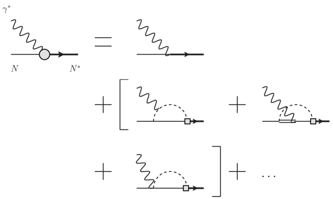
Figure 1: Graphical illustration of the contribution to the $\pi N$ intermediate state to the dressed $\gamma^{*}N\rightarrow N^{*}$ vertex defined by Eq. (LABEL:eq:pw-v).

Within the one-photon exchange approximation, the differential cross sections of pion electroproduction can be written as

$$\frac{d\sigma^{5}}{dE_{e^{\prime}}d\Omega_{e^{\prime}}d\Omega_{\pi}^{*}} = \Gamma_{\gamma}\left[\sigma_{T}+\epsilon\sigma_{L}+\sqrt{2\epsilon(1+\epsilon)}\sigma_{LT}\cos\phi_{\pi}^{\ast}\right.$$ (5)

$$\left.+\epsilon\sigma_{TT}\cos 2\phi_{\pi}^{\ast}+h_{e}\sqrt{2\epsilon(1-\epsilon)}\sigma_{LT^{\prime}}\sin\phi_{\pi}^{\ast}\right].$$

Here $\Gamma_{\gamma}=[\alpha/(2\pi^{2}Q^{2})](E_{e^{\prime}}/E_{e})[|\vec{q}_{L}|/(1-\epsilon)]$; $\epsilon$ is defined by the electron scattering angle $\theta_{e}$ and the photon 3-momentum ${\vec{q}}_{L}$ in the laboratory frame as $\epsilon=[1+2(|\vec{q}_{L}|^{2}/Q^{2})\tan^{2}(\theta_{e}/2)]^{-1}$; $h_{e}$ is the helicity of the incoming electron; $\phi_{\pi}^{\ast}$ is the angle between the $\pi$-$N$ plane and the plane of the incoming and outgoing electrons. The quantities associated with the electrons are defined in the laboratory frame. On the other hand, structure functions of $\gamma^{*}N\to\pi N$ process, $\sigma_{\alpha}=\sigma_{\alpha}(W,Q^{2},\cos\theta_{\pi}^{\ast})$ ($\alpha=T,L,LT,TT,LT^{\prime})$, are defined in the final $\pi N$ center of mass system. The formula for calculating $\sigma_{\alpha}$ from the amplitudes defined by Eqs. (1)-(3) are given in Ref. sl09 .

In this first-stage investigation, we only consider the data of structure functions $\sigma_{\alpha}$ of $p(e,e^{\prime}\pi^{0})p$ m98 ; e1c-pi0ltp and $p(e,e^{\prime}\pi^{+})n$ e1c ; e1c-pipltp up to $W=1.6$ GeV and $Q^{2}=1.45$ (GeV/c)². The availability of the data in the corresponding $(W,Q^{2})$ region are found in Table 1. The resulting parameters are then confirmed against the original five-fold differential cross section data hallb-site . This procedure could overestimate/underestimate the errors of our analysis, but is sufficient for the present exploratory investigation.

Table 1: Available structure function data at $Q^{2}\leq 1.45$ (GeV/c)².

$Q^{2}$ (GeV/c)2	$\gamma^{*}p\to\pi^{0}p$	$\gamma^{*}p\to\pi^{+}n$
$0.3$	——	$\sigma_{T}+\epsilon\sigma_{L},~{}\sigma_{LT},~{}\sigma_{TT}$ e1c
$0.4$	$\sigma_{T}+\epsilon\sigma_{L},~{}\sigma_{LT},~{}\sigma_{TT}$ m98 ; $\sigma_{LT^{\prime}}$ e1c-pi0ltp	$\sigma_{T}+\epsilon\sigma_{L},~{}\sigma_{LT},~{}\sigma_{TT}$ e1c ; $\sigma_{LT^{\prime}}$ e1c-pipltp
$0.5$	——	$\sigma_{T}+\epsilon\sigma_{L},~{}\sigma_{LT},~{}\sigma_{TT}$ e1c
$0.525$	$\sigma_{T}+\epsilon\sigma_{L},~{}\sigma_{LT},~{}\sigma_{TT}$ m98	——
$0.6$	——	$\sigma_{T}+\epsilon\sigma_{L},~{}\sigma_{LT},~{}\sigma_{TT}$ e1c
$0.65$	$\sigma_{T}+\epsilon\sigma_{L},~{}\sigma_{LT},~{}\sigma_{TT}$ m98 ; $\sigma_{LT^{\prime}}$ e1c-pi0ltp	$\sigma_{LT^{\prime}}$ e1c-pipltp
$0.75$	$\sigma_{T}+\epsilon\sigma_{L},~{}\sigma_{LT},~{}\sigma_{TT}$ m98	——
$0.9$	$\sigma_{T}+\epsilon\sigma_{L},~{}\sigma_{LT},~{}\sigma_{TT}$ m98	——
$1.15$	$\sigma_{T}+\epsilon\sigma_{L},~{}\sigma_{LT},~{}\sigma_{TT}$ m98	——
$1.45$	$\sigma_{T}+\epsilon\sigma_{L},~{}\sigma_{LT},~{}\sigma_{TT}$ m98	——

In section II, we present the results from our analysis. Discussions on future developments are given in section III.

II Analysis and Results

To proceed, we need to define the bare $\gamma^{\ast}N\rightarrow N^{*}$ vertex functions $\Gamma^{J}_{N^{*},\lambda_{\gamma}\lambda_{N}}(q,Q^{2})$ of Eq. (LABEL:eq:pw-v). We parameterize these functions as

$${\Gamma}^{J}_{N^{*},\lambda_{\gamma}\lambda_{N}}(q,Q^{2}) = \frac{1}{(2\pi)^{3/2}}\sqrt{\frac{m_{N}}{E_{N}(q)}}\sqrt{\frac{q_{R}}{|q_{0}|}}G_{\lambda}(N^{*},Q^{2})\delta_{\lambda,(\lambda_{\gamma}-\lambda_{N})},$$ (6)

where $q_{R}$ and $q_{0}$ are defined by $M_{N^{*}}=q_{R}+E_{N}(q_{R})$ with $N^{*}$ mass and $W=q_{0}+E_{N}(q_{0})$, respectively, and

$$G_{\lambda}(N^{*},Q^{2}) = A_{\lambda}(N^{*},Q^{2}),~{}~{}~{}\text{for transverse photon},$$ (7)

$$= S_{\lambda}(N^{*},Q^{2}),~{}~{}~{}\,\text{for longitudinal photon}.$$ (8)

For later discussions, we also cast the helicity amplitudes of the dressed vertex Eq. (LABEL:eq:pw-v) into the form of Eq. (6) with dressed helicity amplitudes

$$\bar{A}_{\lambda}(N^{*},Q^{2}) = {A}_{\lambda}(N^{*},Q^{2})+{A}^{\text{m.c.}}_{\lambda}(N^{*},Q^{2}),$$ (9)

$$\bar{S}_{\lambda}(N^{*},Q^{2}) = {S}_{\lambda}(N^{*},Q^{2})+{S}^{\text{m.c.}}_{\lambda}(N^{*},Q^{2}),$$ (10)

where ${A}^{\text{m.c.}}_{\lambda}(N^{*},Q^{2})$ and ${S}^{\text{m.c.}}_{\lambda}(N^{*},Q^{2})$ are due to the meson cloud effect defined by the second term of Eq. (LABEL:eq:pw-v).

With the hadronic parameters of the employed dynamical coupled-channels model determined in analyzing the $\pi N$ reaction data jlms07 ; kjlms09 , the only freedom in analyzing the electromagnetic meson production reactions is the electromagnetic coupling parameters of the model. If the parameters listed in Ref. msl07 are used to calculate the non-resonant interaction ${v}^{J}_{L^{\prime}S^{\prime}M^{\prime}B^{\prime},\lambda_{\gamma}\lambda_{N}}(k^{\prime},q)$ in Eqs. (2) and (LABEL:eq:pw-v), the only parameters to be determined from the data of pion electroproduction reactions are the bare helicity amplitudes defined by Eq. (6). Such a highly constrained analysis was performed in Ref. jlmss08 for pion photoproduction. It was found that the available data of $\gamma p\rightarrow\pi^{0}p,~{}\pi^{+}n$ can be fitted reasonably well up to invariant mass $W\leq 1.6$ GeV. In this work we extend this effort to analyze the pion electroproduction data in the same $W$ region.

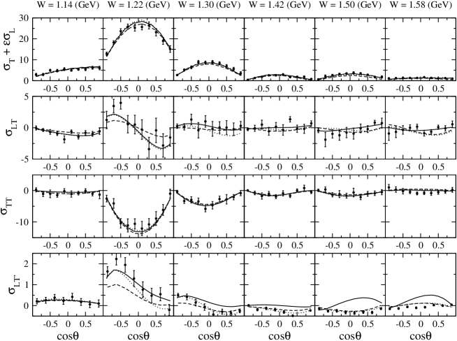
Figure 2: Fit to $p(e,e^{\prime}\pi^{0})p$ structure functions at $Q^{2}=0.4$ (GeV/c)². Here $\theta\equiv\theta_{\pi}^{*}$. The solid curves are the results of Fit1, the dashed curves are of Fit2, and the dotted curves are of Fit3. (See text for the description of each fit.) The data are taken from Refs. m98 ; e1c-pi0ltp .

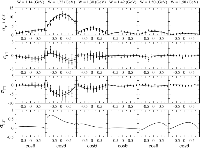
Figure 3: Fit to $p(e,e^{\prime}\pi^{0})p$ structure functions at $Q^{2}=0.9$ (GeV/c)². Here $\theta\equiv\theta_{\pi}^{*}$. The data are taken from Ref. m98 .

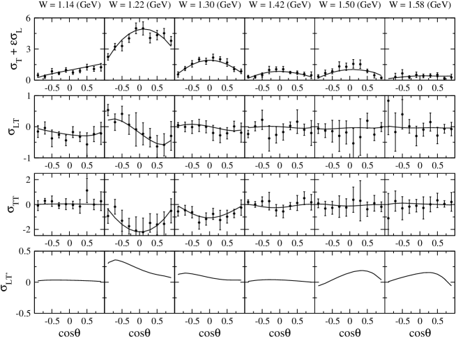
Figure 4: Fit to $p(e,e^{\prime}\pi^{0})p$ structure functions at $Q^{2}=1.45$ (GeV/c)². Here $\theta\equiv\theta_{\pi}^{*}$. The data are taken from Ref. m98 .

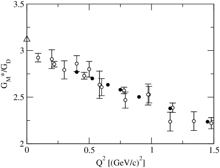
Figure 5: $G_{M}^{\ast}$ normalized by the dipole factor $G_{D}=[1+Q^{2}/0.71\text{(GeV/c)}^{2}]^{-2}$. The solid black circles at $Q^{2}>0$ are our fit to the values extracted from previous analyses (those values are taken from Ref. jlmss08 ). The triangle at $Q^{2}=0$ is from our photoproduction analysis jlmss08 .

We first try to fix the bare helicity amplitudes by fitting to the data of $\sigma_{T}+\epsilon\sigma_{L}$, $\sigma_{LT}$, and $\sigma_{TT}$ of $p(e,e^{\prime}\pi^{0})p$ in Ref. m98 which covers almost all $(W,Q^{2})$ region we are considering (see Table. 1). In a purely phenomenological approach, we first vary all of the helicity amplitudes of 16 bare $N^{*}$ states, considered in analyzing the $\pi N\rightarrow\pi N,\pi\pi N$ data jlms07 ; kjlms09 , in the fits to the data. It turns out that only the helicity amplitudes of the first $N^{*}$ states in $S_{11}$, $P_{11}$, $P_{33}$ and $D_{13}$ are relevant in the considered $W\leq$ 1.6 GeV. Thus in this paper only the bare helicity amplitudes associated with those four bare $N^{*}$ states (total 10 parameters) are varied in the fit and other bare helicity amplitudes are set to zero. The numerical fit is performed at each $Q^{2}$ independently, using the MINUIT library.

The results of our fits are the solid curves in the top three rows of Figs. 2-4. Clearly our results from this fit agree with the data well. We obtain similar quality of fits to the data of Ref. m98 at other $Q^{2}$ values listed in Table. 1. We have also used the magnetic $M1$ form factor of $\gamma^{\ast}N\to\Delta(1232)$ extracted from previous analyses as data for fitting. The results are shown in Fig. 5. We refer the results of this fit to as “Fit1”.

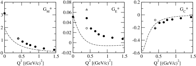
Figure 6: The $\gamma^{\ast}N\to\Delta(1232)$ form factors. Solid points are from Fit1; dashed curves are the meson cloud contribution. Open circles and triangles at $Q^{2}=0.4$ (GeV/c)² are from Fit2 and Fit3, respectively. The three points are almost overlapped in $G_{M}^{\ast}$. The solid point at $Q^{2}=0$ is obtained from the photoproduction reaction analysis in Ref. jlmss08 .

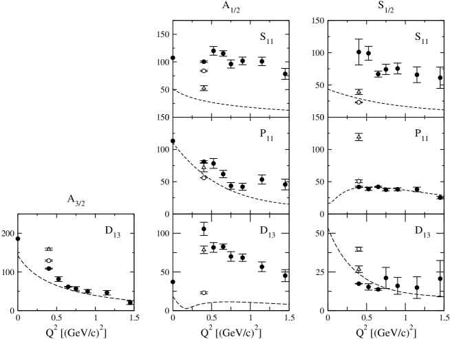
Figure 7: Extracted helicity amplitudes for $S_{11}$ at $W=1535$ MeV (upper panels), $P_{11}$ at $W=1440$ MeV (middle panels), and $D_{13}$ at $W=1520$ MeV (lower panels). The meaning of each point and curve is same as in Fig. 6.

In Fig. 6, we present the $G_{M}^{\ast}$, $G_{E}^{\ast}$, and $G_{C}^{\ast}$ form factors of $\gamma^{\ast}N\to\Delta(1232)$ transition obtained from Fit1 (solid points). In the same figure, we also show the meson cloud effect in the form factors. Within our model, it has a significant contribution at low $Q^{2}$, but rapidly decreases as $Q^{2}$ increases, particularly for $G_{E}^{\ast}$ and $G_{C}^{\ast}$. These results are similar to the previous findings sl01 ; jlss07 .

The helicity amplitudes of $S_{11}$, $P_{11}$, and $D_{13}$ resulting from Fit1 are shown in Fig. 7. The solid circles are the absolute magnitude of the dressed helicity amplitudes (9) and (10). The errors there are assigned by MIGRAD in the MINUIT library. More detailed analysis of the errors is perhaps needed, but will not be addressed here. The meson cloud effect (dashed curves), as defined by $A^{\text{m.c.}}_{\lambda}$ and $S^{\text{m.c.}}_{\lambda}$ of Eqs. (9) and (10) and calculated from the second term of Eq. (LABEL:eq:pw-v), are the necessary consequence of the unitarity conditions. They do not include the bare helicity term determined here and are already fixed in the photoproduction analysis jlmss08 . Within our model (and within Fit1), the meson cloud contribution is relatively small in $S_{11}$ and $A_{1/2}$ of $D_{13}$ even in the low $Q^{2}$ region.

Here we note that our helicity amplitudes defined in Eqs. (9) and (10) are different from the commonly used convention, say $A^{\text{cnv}}_{\lambda}$ and $S^{\text{cnv}}_{\lambda}$, which are obtained from the imaginary part of the $\gamma^{\ast}N\to\pi N$ multipole amplitudes abl08 . This definition leads to helicity amplitudes which are real, while our dressed amplitudes are complex. It was shown in Ref. sl01 that for the $\Delta(1232)$ resonance our dressed helicity amplitudes (9) and (10) can be reduced to $A^{\text{cnv}}_{\lambda}$ and $S^{\text{cnv}}_{\lambda}$, if we replace the Green function $G_{\pi N}$ with its principal value in all loop integrals appearing in the calculation. However, such reduction is not so trivial for higher resonance states because the unstable $\pi\Delta,\rho N,\sigma N$ channels open, and thus the direct comparison of the helicity amplitudes from other analyses becomes unclear.

At $Q^{2}=0.4$ (GeV/c)², the data of all structure functions both for $p(e,e^{\prime}\pi^{0})p$ and $p(e,e^{\prime}\pi^{+})n$ are available as seen in Table. 1. To see the sensitivity of the resulting helicity amplitudes to the amount of the data included in the fits, we further carry out two fits at this $Q^{2}$, referred to as Fit2 and Fit3, respectively. Fit2 (Fit3) further includes the data of Refs. e1c-pi0ltp ; e1c ; e1c-pipltp (Ref. e1c-pi0ltp ) in the fit in addition to those of Ref. m98 which are used in Fit1. This means that Fit2 includes all available data both from $p(e,e^{\prime}\pi^{0})p$ and $p(e,e^{\prime}\pi^{+})n$, whereas Fit3 includes the same data but from $p(e,e^{\prime}\pi^{0})p$ only. The results of each fit are the dashed and dotted curves in Fig. 2 for $p(e,e^{\prime}\pi^{0})p$ and Fig. 8 for $p(e,e^{\prime}\pi^{+})n$, respectively.

The resulting bare helicity amplitudes are listed in the third (Fit2) and fourth (Fit3) columns of Table II and compare with that from Fit1. The corresponding change in the $\gamma N\to\Delta(1232)$ form factors and the dressed helicity amplitudes are also shown as open circles and triangles in Figs. 6 and 7. A significant change among the three different fits is observed in most of the results except $G^{\ast}_{M}$ in $P_{33}$. This indicates that fitting the data listed in Table 1 are far from sufficient to pin down the $\gamma^{*}N\rightarrow N^{*}$ transition form factors up to $Q^{2}=1.45$ (GeV/c)². It clearly indicates the importance of obtaining data from complete or over-complete measurements of most, if not all, of the independent $p(e,e^{\prime}\pi)N$ polarization observables. Such measurements were made by Kelly et al. kelly in the $\Delta$ (1232) region and will be performed at JLab for wide ranges of W and $Q^{2}$ in the next few years bl04 .

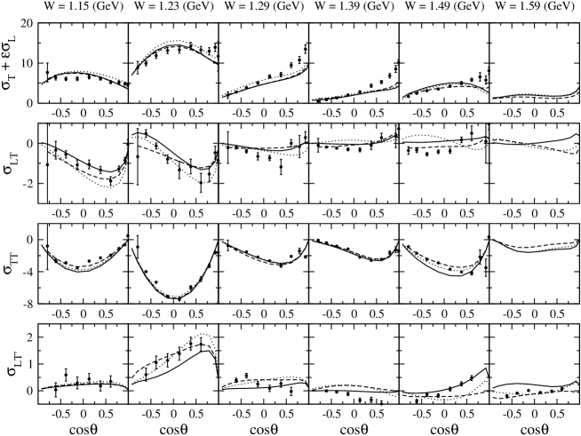
Figure 8: Structure functions of $p(e,e^{\prime}\pi^{+})n$ at $Q^{2}=0.4$ (GeV/c)². Here $\theta\equiv\theta_{\pi}^{*}$. The solid curves are the results of Fit1, the dashed curves are of Fit2, and the dotted curves are of Fit3. (See text for the description of each fit.) As for the $\sigma_{LT^{\prime}}$, results at $W=1.14,1.22,1.3,1.38,1.5,1.58$ GeV (from left to right of the bottom row) are shown, in which the data are available. The data in the figure are taken from Ref. e1c ; e1c-pipltp .

Table 2: Ambiguity of resulting bare helicity amplitudes [the results are at $Q^{2}=0.4$ (GeV/c)²]. The errors are assigned by MIGRAD in the MINUIT library.

	Fit1	Fit2	Fit3
	(Ref. m98 data)	(Refs. m98 ; e1c-pi0ltp ; e1c ; e1c-pipltp data)	(Refs. m98 ; e1c-pi0ltp data)
$S_{11}~{}A_{1/2}$	$100.80\pm 1.46$	$83.25\pm 1.21$	$48.29\pm 5.46$
$S_{11}~{}S_{1/2}$	$-119.30\pm 20.41$	$-9.85\pm 1.69$	$-53.53\pm 4.75$
$P_{11}~{}A_{1/2}$	$33.18\pm 2.11$	$-15.68\pm 1.00$	$20.17\pm 10.37$
$P_{11}~{}S_{1/2}$	$37.29\pm 2.26$	$52.23\pm 3.16$	$131.00\pm 5.87$
$P_{33}~{}A_{3/2}$	$-146.00\pm 0.60$	$-137.50\pm 0.56$	$-150.80\pm 1.03$
$P_{33}~{}A_{1/2}$	$-54.47\pm 0.61$	$-62.57\pm 0.69$	$-46.29\pm 1.73$
$P_{33}~{}S_{1/2}$	$7.85\pm 1.25$	$-7.66\pm 1.22$	$7.34\pm 1.69$
$D_{13}~{}A_{3/2}$	$-44.01\pm 1.31$	$-67.01\pm 1.99$	$-98.63\pm 2.92$
$D_{13}~{}A_{1/2}$	$97.11\pm 8.51$	$14.34\pm 1.26$	$70.02\pm 4.83$
$D_{13}~{}S_{1/2}$	$-18.35\pm 1.37$	$19.43\pm 1.45$	$4.11\pm 2.76$

It has been seen in Fig. 8 that all of our current fits underestimate $\sigma_{T}$ of $p(e,e^{\prime}\pi^{+})n$ at forward angles. We find that this can be improved by further varying the $S_{31}$ and $P_{13}$ bare helicity amplitudes within their reasonable range. In Fig. 9, the results with the nonzero $S_{31}$ and $P_{13}$ bare helicity amplitudes (solid curves) are compared with the results without varying those amplitudes (dashed curves). The resulting values of the bare helicity amplitudes are $(A_{1/2}^{S_{31}},S_{1/2}^{S_{31}})=(121.6,59.6)$ and $(A_{3/2}^{P_{13}},A_{1/2}^{P_{13}},S_{1/2}^{P_{13}})=(-73.2,-42.9,41.5)$. The parameters of Fit2 are used for $S_{11}$, $P_{11}$, $P_{33}$, and $D_{13}$ in both curves. In the figure we have just shown the results at $W\sim 1.3$ GeV. We confirm that the same consequence is obtained also at other $W$, and find that the $P_{13}$ ($S_{31}$) has contributions mainly at low (high) $W$. We also find that the inclusion of the bare $S_{31}$ and $P_{13}$ helicity amplitudes does not change other structure functions than $\sigma_{T}$ of $p(e,e^{\prime}\pi^{+})n$ (at most, most of the change is within the error). This indicates that those two helicity amplitudes are rather relevant to $p(e,e^{\prime}\pi^{+})n$, but not to $p(e,e^{\prime}\pi^{0})p$. As shown in Table 1, however, no enough data is currently available for $p(e,e^{\prime}\pi^{+})n$ above $Q^{2}=0.4$ (GeV/c)². The data both of the $p(e,e^{\prime}\pi^{0})p$ and $p(e,e^{\prime}\pi^{+})n$ at same $Q^{2}$ values are desirable to pin down the $Q^{2}$ dependence of the $S_{31}$ and $P_{13}$ helicity amplitudes.

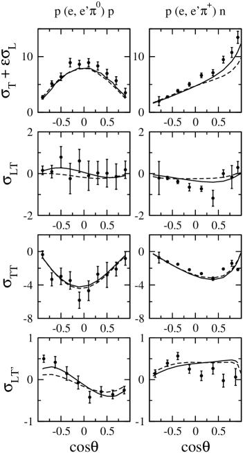
Figure 9: Contribution of the $S_{31}$ and $P_{13}$ helicity amplitudes at $Q^{2}=0.4$ (GeV/c)². The left (right) panels are the structure functions of $p(e,e^{\prime}\pi^{0})p$ [$p(e,e^{\prime}\pi^{+})n$] reaction at $W=1.3$ GeV ($W=1.29$ GeV). Solid (dashed) curves are the results with (without) nonzero $S_{31}$ and $P_{13}$ bare helicity amplitudes. The parameters of Fit2 are used for the $S_{11}$, $P_{11}$, $P_{33}$, and $D_{13}$ helicity amplitudes in both curves. The data are from Refs. m98 ; e1c-pi0ltp ; e1c ; e1c-pipltp .

We now turn to show the coupled-channels effect. In Fig. 10, we see that when only the $\pi N$ intermediate state is kept in the $M^{\prime}B^{\prime}$ summation of the non-resonant amplitude [Eq. (2)] and the dressed $\gamma^{*}N\to N^{*}$ vertices [Eq. (LABEL:eq:pw-v)], the predicted total transverse and longitudinal cross sections $\sigma_{T}$ and $\sigma_{L}$ of $p(e,e^{\prime}\pi^{0})p$ are changed from the solid to dashed curves. This corresponds to only examining the coupled-channels effect on the electromagnetic ($Q^{2}$-dependent) part in the $\gamma^{\ast}N\to\pi N$ amplitude. All coupled-channels effects on the non-electromagnetic interactions are kept in the calculations. We find that the coupled-channels effect tends to decrease when $Q^{2}$ increases. This is rather clearly seen in $\sigma_{T}$. In particular, the coupled-channels effect on $\sigma_{T}$ at high $W\sim 1.5$ GeV is small ($10$-$20$%) already at $Q^{2}=0.4$ (GeV/c)². (The effect is about $30$-$40$% at $Q^{2}=0$ jlmss08 .) This is understood as follows. In Eq. (3) we can further split the resonant amplitude $t^{R}$ as $t^{R}=t^{R}_{\text{bare}}+t^{R}_{\text{m.c.}}$, where $t^{R}_{\text{bare}}$ and $t^{R}_{\text{m.c.}}$ are the same as $t^{R}$ but replacing $\bar{\Gamma}^{J}_{N^{\ast},\lambda_{\gamma}\lambda_{N}}$ with its bare part $\Gamma^{J}_{N^{\ast},\lambda_{\gamma}\lambda_{N}}$ and meson cloud part [the second term of Eq. (LABEL:eq:pw-v)], respectively. The coupled-channels effect shown in Fig. 10 comes from $t^{J}_{LS_{N}\pi N,\lambda_{\gamma}\lambda_{N}}$ and $t^{R}_{\text{m.c.}}$. We have found that the relative importance of the coupled-channels effect in each part remains the same for increasing $Q^{2}$. However, the contribution of non-resonant mechanisms both on $t^{J}_{LS_{N}\pi N,\lambda_{\gamma}\lambda_{N}}$ and $t^{R}_{\text{m.c.}}$ to the structure functions decreases for higher $Q^{2}$ compared with $t^{R}_{\text{bare}}$. This explains the smaller coupled-channels effect compared with the photoproduction reactions jlmss08 . The decreasing non-resonant interaction at higher $Q^{2}$ is due to its long range nature, thus indicating that higher $Q^{2}$ reactions provide a clearer probe of $N^{\ast}$. We obtain similar results also for $p(e,e^{\prime}\pi^{+})n$.

It is noted, however, that the above argument does not mean coupled-channels effect is negligible in the full $\gamma^{\ast}N\to\pi N$ reaction process. In the above analysis we kept the coupled-channels effect on the hadronic non-resonant amplitudes, the strong $N^{\ast}$ vertices, and the $N^{\ast}$ self-energy, which are $Q^{2}$-independent and remain important irrespective of $Q^{2}$. We have found in the previous analyses jlms07 ; kjlms09 that the coupled-channels effect on them is significant in all energy region up to $W=2$ GeV.

In Fig. 11, we show the coupled-channels effect on the five-fold differential cross section defined by Eq. (5). The coupled-channels effects are significant at low $W$, whereas they are small at high $W$. This is consistent with the above discussions because the five-fold differential cross sections are dominated by $\sigma_{T}$. Here we also see that our full results (solid curves) are in good agreement with the original data, although we performed the fits by using the structure function data listed in Table 1.

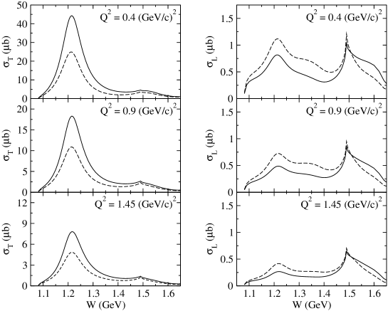
Figure 10: Coupled-channels effect on the integrated structure functions $\sigma_{T}(W)$ and $\sigma_{L}(W)$ for $Q^{2}=0.4,~{}0.9,~{}1.45$ (GeV/c)² for $p(e,e^{\prime}\pi^{0})p$ reactions. The solid curves are the full results calculated with the bare helicity amplitudes of Fit1. The dashed curves are the same as solid curves but only the $\pi N$ loop is taken in the $M^{\prime}B^{\prime}$ summation in Eqs. (2) and (LABEL:eq:pw-v).

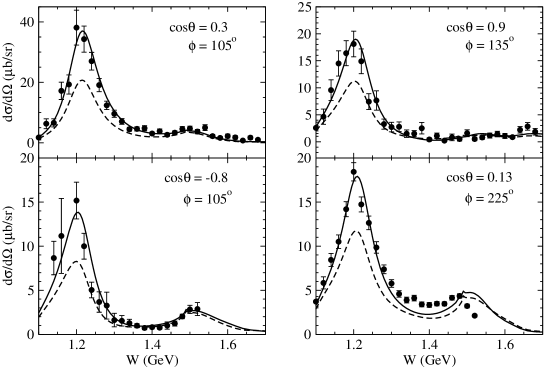
Figure 11: Coupled-channels effect on the five-fold differential cross sections $\Gamma_{\gamma}^{-1}[d\sigma^{5}/(dE_{e^{\prime}}d\Omega_{e^{\prime}}d\Omega_{\pi}^{*})]$ of $p(e,e^{\prime}\pi^{0})p$ (upper panels) and $p(e,e^{\prime}\pi^{+})n$ (lower panels) at $Q^{2}=0.4$ (GeV/c)². Here $\theta\equiv\theta_{\pi}^{*}$ and $\phi\equiv\phi_{\pi}^{*}$. The solid curves are the full results calculated with the bare helicity amplitudes of Fit1. The dashed curves are the same as the solid curves but only the $\pi N$ loop is taken in the $M^{\prime}B^{\prime}$ summation in Eqs. (2) and (LABEL:eq:pw-v). The data are taken from Ref. hallb-site

.

III Summary and outlook

In this work we have explored how the available $p(e,e^{\prime}\pi)N$ data can be used to determine the $\gamma^{*}N\rightarrow N^{*}$ transition form factors within a dynamical coupled-channels models msl07 ; jlms07 ; jlmss08 ; djlss08 ; kjlms09 . Within the available data, the $\gamma^{*}N\rightarrow N^{*}$ bare helicity amplitudes of the first $N^{*}$ states in $S_{11}$, $P_{11}$, $P_{33}$ and $D_{13}$ can be determined in the considered energy region $W\leq$ 1.6 GeV. We further observe that some of these parameters can not be determined well. The uncertainties could be due to the limitation that only data of 4 out of 11 independent $p(e,e^{\prime}\pi)N$ observables are available for our analysis. Clearly, the data from the forthcoming measurements of double and triple polarization observables at JLab will be highly desirable to make progress.

Also, it was found that the underestimation of the $\sigma_{T}$ of $p(e,e^{\prime}\pi^{+})n$ at forward angles can be improved by further considering the $S_{31}$ and $P_{13}$ bare helicity amplitudes. Furthermore, these amplitudes can have relevant contribution to $p(e,e^{\prime}\pi^{+})n$, but not to $p(e,e^{\prime}\pi^{0})p$. The $p(e,e^{\prime}\pi^{+})n$ data of wide $Q^{2}$ region as well as $p(e,e^{\prime}\pi^{0})p$ seem necessary for determining the $Q^{2}$ dependence of the $S_{31}$ and $P_{13}$ helicity amplitudes.

For testing theoretical predictions from hadron structure calculations such as LQCD, the quantities of interest are the residues of the $\gamma^{*}N\rightarrow\pi N$ amplitudes, defined by Eqs. (1)-(LABEL:eq:pw-v), at the corresponding resonance poles. If the resonance poles are associated with the amplitude $t^{R,J}_{LS_{N}\pi N,\lambda_{\gamma}\lambda_{N}}(k,q,W,Q^{2})$ of Eq. (3), the extracted residues are directly related to the dressed form factors $\bar{\Gamma}^{J}_{N^{*},L^{\prime}S^{\prime}M^{\prime}B^{\prime}}(k^{\prime},W)$. An analytic continuation method for extracting these information has been developed ssl09 , and our results along with other hadronic properties associated nucleon resonances will be published elsewhere. Here we only mention that the extracted form factors are complex and some investigations are needed to see how they can be compared with the helicity amplitudes, which are real numbers, listed by PDG pdg . In a Hamiltonian formulation as taken in our dynamical approach, the physical meanings of poles and residues are well defined in textbooks goldberger ; feshbach .

References

(1)
V. Burkert and T.-S. H. Lee, Int.
J. of Mod. Phys. E13, 1035 (2004).
(2)
A. Matsuyama, T. Sato, and T.-S. H. Lee,
Phys. Rep. 439, 193 (2007).
(3)
B. Juliá-Díaz, T.-S. H. Lee, A. Matsuyama, and T. Sato,
Phys. Rev. C 76, 065201 (2007).
(4)
B. Juliá-Díaz, T.-S. H. Lee, A. Matsuyama, T. Sato, and L. C. Smith,
Phys. Rev. C 77, 045205 (2008).
(5)
J. Durand, B. Juliá-Díaz, T.-S. H. Lee, B. Saghai, and T. Sato,
Phys. Rev. C 78, 025204 (2008).
(6)
H. Kamano, B. Juliá-Díaz, T.-S. H. Lee, A. Matsuyama, and T. Sato,
Phys. Rev. C 79, 025206 (2009).
(7)
B. Juliá-Díaz, T.-S. H. Lee, T. Sato, and L. C. Smith,
Phys. Rev. C 75, 015205 (2007).
(8)
T. Sato and T.-S. H. Lee,
Phys. Rev. C 54, 2660 (1996).
(9)
T. Sato and T.-S. H. Lee,
J. Phys. G 36, 073001 (2009).
(10)
K. Joo et al. (CLAS Collaboration),
Phys. Rev. Lett. 88, 122001 (2002).
(11)
K. Joo et al. (CLAS Collaboration),
Phys. Rev. C 68, 032201 (2003).
(12)
H. Egiyan et al. (CLAS Collaboration),
Phys. Rev. C 73, 025204 (2006).
(13)
K. Joo et al. (CLAS Collaboration),
Phys. Rev. C 72, 058202 (2005).