A Study of Channel Estimation and Postprocessing
in Quantum Key Distribution Protocols

Shun Watanabe

Supervisor: Prof. Ryutaroh Matsumoto

A Thesis submitted for the degree of Doctor of Philosophy

Department of Communications and Integrated Systems

Tokyo Institute of Technology

2009

Abstract

Quantum key distribution (QKD) has attracted great attention as an unconditionally secure key distribution scheme. The fundamental feature of QKD protocols is that the amount of information gained by an eavesdropper, usually referred to as Eve, can be estimated from the channel between the legitimate sender and the receiver, usually referred to as Alice and Bob respectively. Such a task cannot be conducted in classical key distribution schemes. If the estimated amount is lower than a threshold, then Alice and Bob determine the length of a secret key from the estimated amount of Eve’s information, and can share a secret key by performing the postprocessing. One of the most important criteria for the efficiency of the QKD protocols is the key generation rate, which is the length of securely sharable key per channel use.

In this thesis, we investigate the channel estimation procedure and the postprocessing procedure of the QKD protocols in order to improve the key generation rates of the QKD protocols. Conventionally in the channel estimation procedure, we only use the statistics of matched measurement outcomes, which are bit sequences transmitted and received by the same basis, to estimate the channel; mismatched measurement outcomes, which are bit sequences transmitted and received by different bases, are discarded in the conventional estimation procedure. In this thesis, we propose a channel estimation procedure in which we use the mismatched measurement outcomes in addition to the matched measurement outcomes. Then, we clarify that the key generation rates of the QKD protocols with our channel estimation procedure is higher than that with the conventional channel estimation procedure.

In the conventional postprocessing procedure, which is known as the advantage distillation, we transmit a message over the public channel redundantly, which is unnecessary divulging of information to Eve. In this thesis, we propose a postprocessing in which the above mentioned divulging of information is reduced by using the distributed data compression. We clarify that the key generation rate of the QKD protocol with our proposed postprocessing is higher than that with the conventionally known postprocessings.

Contents

1. 1 Introduction
   1. 1.1 Background
   2. 1.2 Key Agreement in Information Theory
   3. 1.3 Unique Property of Quantum Key Distribution
   4. 1.4 Summary
2. 2 Preliminaries
   1. 2.1 Elements of Classical and Quantum Information Theory
      1. 2.1.1 Probability Distribution and Density Operator
      2. 2.1.2 Distance and Fidelity
      3. 2.1.3 Entropy and its Related Quantities
      4. 2.1.4 Bloch Sphere, Choi Operator, and Stokes Parameterization
   2. 2.2 Privacy Amplification
      1. 2.2.1 Min- and Max- Entropy
      2. 2.2.2 Privacy Amplification
3. 3 Channel Estimation
   1. 3.1 Background
   2. 3.2 BB84 and Six-State Protocol
   3. 3.3 One-Way Information Reconciliation
   4. 3.4 Channel Estimation and Asymptotic Key Generation Rate
      1. 3.4.1 Channel Estimation Procedure
      2. 3.4.2 Sufficient Condition on Key Generation Rates for Secure Key Agreement
      3. 3.4.3 Asymptotic Key Generation Rate of The Six-State Protocol
      4. 3.4.4 Asymptotic Key Generation Rate of The BB84 Protocol
   5. 3.5 Comparison to Conventional Estimation
      1. 3.5.1 Six-State Protocol
      2. 3.5.2 BB84 Protocol
   6. 3.6 Asymptotic Key Generation Rates for Specific Channels
      1. 3.6.1 Amplitude Damping Channel
      2. 3.6.2 Unital Channel and Rotation Channel
   7. 3.7 Condition for Strict Improvement
   8. 3.8 Summary
4. 4 Postprocessing
   1. 4.1 Background
   2. 4.2 Advantage Distillation
   3. 4.3 Two-Way Information Reconciliation
   4. 4.4 Security and Asymptotic Key Generation Rate
      1. 4.4.1 Sufficient Condition on Key Generation Rate for Secure Key Agreement
      2. 4.4.2 Asymptotic Key Generation Rates
   5. 4.5 Comparison of Asymptotic Key Generation Rates for Specific Channels
      1. 4.5.1 Pauli Channel
      2. 4.5.2 Unital Channel
      3. 4.5.3 Amplitude Damping Channel
   6. 4.6 Relation to Entanglement Distillation Protocol
   7. 4.7 Summary
5. 5 Conclusion
6. A Notations
7. B Publications Related to This Thesis

Chapter 1 Introduction

1.1 Background

Key distribution is one of the most important and challenging problem in cryptology. When a sender wants to transmit a confidential message to a receiver, the sender usually encipher the message by using a secret key that is only available to the sender and the receiver. For a long time, many methods have been proposed to solve the key distribution problem. One of the most broadly used method in the present day is a method whose security is based on difficulties to solve some mathematical problems, such as factorization into prime numbers. Such kind of method is believed to be practically secure, but it has not been proved to be unconditionally secure; there might exist some clever algorithm to solve those mathematical problems efficiently. On the other hand, quantum key distribution (QKD), which is the main theme of this thesis, has attracted the attention of many researchers, for the reason that its security is based on principles of the quantum mechanics. In other word, the QKD is secure as long as the quantum mechanics is correct.

The concept of the quantum cryptography was proposed by Wiesner in 1970s. Unfortunately, his paper was rejected by a journal, and was not published until 1983 [Wie83]. In 1980s, the quantum cryptography was revived by Bennett et al. in a series of papers [BBBW82, BB83, BB84b, BB84a]. Especially, the quantum key distribution first appeared in Bennett and Brassard’s one page proceedings paper [BB83] presented at a conference, although it is more commonly known as BB84 from its 1984 full publication [BB84a].

At first, the security of the BB84 protocol was guaranteed only in the ideal situation such that the channel between the sender and receiver is noiseless. Later, Bennett et al. proposed modified protocols to handle the case in which the channel between the sender and the receiver is not necessarily noiseless [BB89, BBB⁺92]. During the course of their struggle against the problem, many important concepts such as the information reconciliation and the privacy amplification, which are explained in detail later, were proposed [BBR85, BBR88]. Finally , Mayers proposed his version of the BB84 protocol, and showed its unconditional security [May01] (preliminary versions of his proof were published in [May95, May96]). Biham et al. also proposed their version of the BB84 protocol and showed its unconditional security [BBB⁺00, BBB⁺06].

In 2000, Shor an Preskill made a remarkable observation on Mayer’s security proof of the BB84 protocol [SP00]. They observed that the entanglement distillation protocol (EDP) [BBP⁺96, LC99] with the CSS code, one of the quantum error correcting codes proposed by Calderbank, Shor, and Stean [CS96, Ste96], is implicitly used in Mayer’s version of the BB84 protocol, and presented a simple proof of Mayer’s version of the BB84 protocol. Their proof technique based on the CSS code is further extended to some directions. For example, Lo [Lo01] proved the security of another QKD protocol, the six state protocol proposed by Bruß [Bru98], by using the technique based on the CSS code.

Recently, Renner et al. [RGK05, Ren05, KGR05] developed information theoretical techniques to prove the security of the QKD protocols including the BB84 protocol and the six-state protocol. Their proof method provides important insight into the security proof of the QKD protocols. More precisely, they proved the security of the QKD protocols by extending the key agreement in the information theory [Mau93, AC93], which will be explained in the next section, to the context of the QKD protocols.

In this thesis, we employ Renner et al.’s approach for the security proof of the QKD protocols instead of Shor and Preskill’s approach. Then, we investigate two important phases, the channel estimation and the postprocessing, of the QKD protocols.

The QKD protocol roughly consists of three phases: the bit transmission phase, the channel estimation phase, and the postprocessing phase. In the bit transmission phase, the legitimate sender, usually referred to as Alice sends a bit sequence to the legitimate receiver, usually referred to as Bob, by encoding them into quantum carrier (eg. polarizations of photons). The channel estimation phase will be explained in Section 1.3. In the postprocessing phase, Alice and Bob share a secret key based on their bit sequences obtained in the bit transmission phase. The postprocessing phase can be essentially regarded as the key agreement problem in the information theory, which will be explained in the next section.

1.2 Key Agreement in Information Theory

Following Shannon’s mathematical formulation of the cryptography [Sha48] and the studies on confidential message transmissions over noisy channels by Wyner [Wyn75] and Csisźar and Körner [CK79], the problem of the key agreement in the information theory was formulated by Maurer [Mau93], and was also studied by Ahlswede and Csisźar [AC93].

In Maurer’s formulation Alice and Bob have sequences of independently identically distributed (i.i.d.) correlated binary random variables $\mathbf{X}=(X_{1},\ldots,X_{n})$ and $\mathbf{Y}=(Y_{1},\ldots,Y_{n})$ respectively, and the eavesdropper, usually referred to as Eve, has a sequence of i.i.d. random variables $\mathbf{E}=(E_{1},\ldots,E_{n})$, which are regarded as the information she obtained by eavesdropping $\mathbf{X}$ and $\mathbf{Y}$. They conduct a postprocessing procedure and share a secret key by using the pair of bit sequence $(\mathbf{X},\mathbf{Y})$ as a seed.

In the postprocessing procedure, Alice and Bob are allowed to exchange messages over the authenticated public channel, that is, Eve can know every message transmitted over this channel but she cannot tamper or forge a message. Actually, the authenticated public channel can be realized if Alice and Bob initially share a short secret key [Sti91]. In the rest of this thesis, we assume that the public channel is always authenticated though we do not mention it explicitly.

The communication over the public channel in the postprocessing procedure may be one-way (from Alice to Bob) or two-way. The most elementary postprocessing procedure is a procedure with one-way public communication, and it consists of two procedures, the information reconciliation procedure and the privacy amplification procedure.

The purpose of the information reconciliation procedure for Alice and Bob is to agree on a bit sequence from their correlated bit sequences. This procedure is nothing but the Slepian-Wolf coding scheme [SW73]. In this scheme, Alice sends the compressed version $C$ (say $k$ bit data) of $\mathbf{X}$ to Bob. Then, Bob reproduce $\hat{\mathbf{X}}$ by using his bit sequence $\mathbf{Y}$ and the received data $C$. It is well known that Bob can reproduce Alice’s bit sequence with negligible error probability if Alice sends appropriate $k\simeq nH(X|Y)$ bits data.

The purpose of the privacy amplification procedure for Alice and Bob is to distill secret keys from their bit sequences shared in the information reconciliation procedure. More specifically, Alice and Bob distill $\ell$ bits (usually much shorter than $n$ bit) secret key by using appropriate function from $n$ bit to $\ell$ bit. We require the secret keys to be information theoretically secure, i.e., the distilled key is uniformly distributed and statistically independent from Eve’s available information $C$ and $\mathbf{E}$.

Since the pair of bit sequences initially shared by Alice and Bob are considered as a precious resource, we desire the key generation rate $\ell/n$ to be as large as possible. Especially in this paper, we investigate the asymptotic behavior of the key generation rate, asymptotic key generation rate, such that the secure key agreement is possible. Roughly speaking, the secure key can be distilled if the key generation rate is smaller than Eve’s ambiguity (per bit) about the bit sequence after the information reconciliation, that is,

$$\frac{\ell}{n}\overset{<}{\sim}H(X|E)-H(X|Y).$$ (1.1)

In [Mau93], Maurer also proposed a postprocessing procedure with two-way public communication. More specifically, he proposed a preprocessing called advantage distillation that is conducted before the information reconciliation procedure. In the advantage distillation, Alice divides her bit sequence into blocks of length $2$, and sends the parity $X_{2i-1}\oplus X_{2i}$ of each block to Bob. Bob also divides his bit sequence into blocks of length $2$, and tells Alice whether the received parity of the $i$th block coincides with Bob’s corresponding parity $Y_{2i-1}\oplus Y_{2i}$. If their corresponding parities coincide, they keep the second bits of those blocks, which are regarded to have strong correlation. Otherwise, they discard those blocks, which are regarded to have weak correlation. Maurer showed that the key generation rate of the postprocessing with the advantage distillation can be strictly higher than the right hand side of Eq. (1.1) in an example.

In the context of the QKD protocol, the postprocessing procedure with both one-way and two-way public communication were considered. Actually, the postprocessing procedure with one-way public communication were first studied [May01, SP00]. Later, the postprocessing with the advantage distillation in the context of QKD protocol was proposed by Gottesman and Lo [GL03]. The postprocessing with the advantage distillation was extensively studied by Bae and Acín [BA07].

In Chapter 4, we propose a new kind of postprocessing procedure with two-way public communication in the context of QKD protocol. The purpose of the advantage distillation was to divide the blocks into highly correlated ones and weakly correlated ones by exchanging the parities. The key idea of our proposed postprocessing is that the parities in the conventional advantage distillation is redundantly transmitted over the public channel, and should be compressed by the Slepian-Wolf coding because Bob’s bits $(Y_{2i-1},Y_{2i})$ is correlated to Alice’s parity $X_{2i-1}\oplus X_{2i}$. In our proposed postprocessing, Alice does not sends the parities itself, but she sends the compressed version of the parities by regarding Bob’s sequence $\mathbf{Y}$ as the side-information at the decoder. This enables Alice and Bob to extract a secret key also from the parity sequence, and improves the key generation rate. Actually, the key generation rate of the QKD protocols with our proposed postprocessing procedure is as high as that with conventional one-way or two-way postprocessing procedures. We also clarify that the former is strictly higher than the latter in some cases.

1.3 Unique Property of Quantum Key Distribution

In the previous section, we have explained the mathematical formulation of the key agreement in the information theory. Then, we have explained the fact that Alice and Bob have to set the key generation rate according Eve’s ambiguity about the bit sequence after the information reconciliation procedure (Eq. (1.1)) in order to share an information theoretically secure key. However, Alice and Bob cannot calculate the amount of Eve’s ambiguity about the bit sequence if they do not know the probability distribution $P_{XYE}$ of their initial bit sequence and Eve’s available information. Therefore, they have to estimate the probability distribution itself, or at least they have to estimate a lower bound on the quantity $H(X|E)$. If Alice and Bob’s bit sequences $(\mathbf{X},\mathbf{Y})$ are distributed by using a classical channel, for example the standard telephone line or the Internet, then a valid estimate will be the trivial one, $0$, because Eve can eavesdrop as much as she want without being detected. The QKD protocols provide a way to estimate a non-trivial lower bound on $H(X|E)$ by using the axioms of the quantum mechanics.

In the BB84 protocol, Alice randomly chooses a bit sequence and send it by encoding each bit into a polarization of a photon. When she encodes each bit into a polarization of a photon, she chooses one of two encoding rules at random. In the first encoding rule, she encodes $0$ into the vertical polarization, and $1$ into the horizontal polarization. In the second encoding rule, she encodes $0$ into the $45$ degree polarization, and $1$ into the $135$ degree polarization.

On the other hand, Bob measures the received photons by using one of two measurement device at random. The first measurement device discriminate between the vertical and the horizontal polarizations, and the measurement outcome is decoded into the corresponding bit value. The second measurement device discriminate between the $45$ degree and the $135$ degree polarizations, and the measurement outcome is decoded into the corresponding bit value.

After the reception of the photons, Alice and Bob announce over the public channel which encoding rule and which measurement device they have used for each bit. Then, they keep those bits if their encoding rule and measurement device are compatible, i.e., Alice uses the first (the second) encoding rule and Bob uses the first (the second) measurement device. We call such bit sequences the matched measurement outcomes. On the other hand, they discard those bits if their encoding rule and measurement device are incompatible, i.e., Alice uses the first (the second) encoding rule and Bob uses the second (the first) measurement device. We call such bit sequences the mismatched measurement outcomes. Furthermore, Alice and Bob announce a part of their matched measurement outcomes to estimate candidates of the quantum channel over which the photons were transmitted. The rest of the matched measurement outcomes are used as a seed for sharing a secret key.

The most important feature of the QKD protocols is that we can calculate the quantity $H(X|E)$ by using the axioms of the quantum mechanics if they know the quantum channel exactly. Therefore, we can estimate a lower bound on $H(X|E)$ via estimating the candidates of the quantum channel. Actually, we employ the quantity $H(X|E)$ minimized over the estimated candidates of the quantum channel as an estimate of true $H(X|E)$.

As we explained above, in the conventional BB84 protocol we discard the mismatched measurement outcomes and we estimate the candidates of the quantum channel by using only the samples from the matched measurement outcomes. In Chapter 3, we propose a channel estimation procedure in which we use the mismatched measurement outcomes in addition to the samples from the matched measurement outcomes. The use of the mismatched measurement outcomes enables us to reduce candidates of the quantum channel, and then enables us to estimate tighter lower bounds on the quantity $H(X|E)$. Actually, we clarify that the key generation rate decided according to our proposed channel estimation procedure is at least as high as the key generation rate decided according to the conventional channel estimation procedure. We also clarify that the former is strictly higher than the latter in some cases. In Chapter 4, we also apply our proposed channel estimation procedure to the protocol with the two-way postprocessing proposed in Chapter 4.

It should be noted that the use of the mismatched measurement outcomes was already considered in literatures. In early 90s, Barnett et al. [BHP93] showed that the use of mismatched measurement outcomes enables Alice and Bob to detect the presence of Eve with higher probability for the so-called intercept and resend attack. Furthermore, some literatures use the mismatched measurement outcomes to ensure the quantum channel to be a Pauli channel [BCE⁺03, LKE⁺03, KLO⁺05, KLKE05], where a Pauli channel is a channel over which four kinds of Pauli errors (including the identity) occur probabilistically. However the quantum channel is not necessarily a Pauli channel in general. One of the aims of this thesis is to convince the readers that the non-Pauli channels deserve consideration in the research of the QKD protocols as well as the Pauli channel.

1.4 Summary

The QKD protocols consists of three phases: the bit transmission phase, the channel estimation phase, and the postprocessing phase. The role of the channel estimation phase is to estimate the amount of Eve’s ambiguity about the bit sequence transmitted in the bit transmission phase. According to the estimated amount of Eve’s ambiguity, we decide the key generation rate and conduct the postprocessing to share a secret key.

In the conventional estimation procedure, we do not use the mismatched measurement outcomes. By using the mismatched measurement outcomes in addition to the samples from the matched measurement outcomes, we can improve the key generation rate of the QKD protocols. This topic is investigated in Chapter 3.

In the conventional (two-way) postprocessing procedure, we transmit a message over the public channel redundantly, which is unnecessary divulging of information to Eve. By transmitting the compressed version of the redundantly transmitted message, we can improve the key generation rate of the QKD protocols. This topic is investigated in Chapter 4.

Chapter 2 Preliminaries

In this chapter, we introduce some terminologies and notations, and give a brief review of the known results that are used throughout this thesis. The first section is devoted to a review of the classical information theory [CT06] and the quantum information theory [NC00, Hay06]. In the second section, we review the known results on the privacy amplification, which is the most important tool for the security of the QKD protocols.

2.1 Elements of Classical and Quantum Information Theory

2.1.1 Probability Distribution and Density Operator

For a finite set ${\cal X}$, let ${\cal P}({\cal X})$ be the set of all probability distributions $P$ on ${\cal X}$, i.e., $P(x)\geq 0$ for all $x\in{\cal X}$ and $\sum_{x\in{\cal X}}P(x)=1$. For a sequence $\mathbf{x}=(x_{1},\ldots,x_{n})\in{\cal X}^{n}$, the type of $\mathbf{x}$ is the empirical probability distribution $P_{\mathbf{x}}\in{\cal P}({\cal X})$ defined by

$$P_{\mathbf{x}}(a):=\frac{|\{i\mid x_{i}=a\}|}{n}~{}~{}~{}~{}~{}~{}\mbox{for }a\in{\cal X},$$

where $|A|$ is the cardinality of a set $A$.

For a finite-dimensional Hilbert space ${\cal H}$, let ${\cal P}({\cal H})$ be the set of all density operators $\rho$ on ${\cal H}$, i.e., $\rho$ is non-negative and normalized, $\mathrm{Tr}\rho=1$. Mathematically, a state of a quantum mechanical system with $d$-degree of freedom is represented by a density operator on ${\cal H}$ with $\dim{\cal H}=d$. Throughout the thesis, we occasionally call $\rho$ a state and ${\cal H}$ a system. For Hilbert spaces ${\cal H}_{A}$ and ${\cal H}_{B}$, the set of all density operators ${\cal P}({\cal H}_{A}\otimes{\cal H}_{B})$ on the tensor product space ${\cal H}_{A}\otimes{\cal H}_{B}$ is defined in a similar manner. In Section 2.2, we occasionally treat non-normalized non-negative operators. For this reason, we denote the set of all non-negative operators on a system ${\cal H}$ (and a composite system ${\cal H}_{A}\otimes{\cal H}_{B}$) by ${\cal P}^{\prime}({\cal H})$ (and ${\cal P}^{\prime}({\cal H}_{A}\otimes{\cal H}_{B})$).

The classical random variables can be regarded as a special case of the quantum states. For a random variable $X$ with a distribution $P_{X}\in{\cal P}({\cal X})$, let

$$\rho_{X}:=\sum_{x\in{\cal X}}P_{X}(x)|x\rangle\langle x|,$$

where $\{|x\rangle\}_{x\in{\cal X}}$ is an orthonormal basis of ${\cal H}_{X}$. We call $\rho_{X}$ the operator representation of the classical distribution $P_{X}$.

When a quantum system ${\cal H}_{A}$ is prepared in a state $\rho^{x}_{A}$ according to a realization $x$ of a random variable $X$ with a probability distribution $P_{X}$, it is convenient to describe this situation by a density operator

$$\rho_{XA}:=\sum_{x\in{\cal X}}P_{X}(x)|x\rangle\langle x|\otimes\rho_{A}^{x}\in{\cal P}({\cal H}_{X}\otimes{\cal H}_{A}),$$ (2.1)

where $\{|x\rangle\}_{x\in{\cal X}}$ is an orthonormal basis of ${\cal H}_{X}$. We call the density operator $\rho_{XA}$ a $\{cq\}$-state [DW05], or we say $\rho_{XA}$ is classical on ${\cal H}_{X}$ with respect to the orthonormal basis $\{|x\rangle\}_{x\in{\cal X}}$. We call $\rho_{A}^{x}$ a conditional operator. When a quantum system ${\cal H}_{A}$ is prepared in a state $\rho_{A}^{x,y}$ according to a joint random variable $(X,Y)$ with a probability distribution $P_{XY}$, a state $\rho_{XYA}$ is defined in a similar manner, and the state $\rho_{XYA}$ is called a $\{ccq\}$-state. For non-normalized operator $\rho_{XA}\in{\cal P}^{\prime}({\cal H}_{X}\otimes{\cal H}_{A})$, if we can write $\rho_{XA}$ as in Eq. (2.1), we say that $\rho_{XA}$ is classical on ${\cal H}_{X}$ with respect to the orthonormal basis $\{|x\rangle\}_{x\in{\cal X}}$. However, it should be noted that the distribution $P_{X}$ or conditional operators $\rho_{A}^{x}$ are not necessarily normalized for a non-normalized $\rho_{XA}$.

For a $\{cq\}$-state $\rho_{XA}\in{\cal P}({\cal H}_{X}\otimes{\cal H}_{A})$, we occasionally consider a density operator such that the classical system ${\cal H}_{X}$ is mapped by a function $f:{\cal X}\to{\cal Y}$. By setting the distribution

$$P_{Y}(y)=\sum_{x\in{\cal X}\atop f(x)=y}P_{X}(x)$$

and the density operator

$$\rho_{A}^{y}=\sum_{x\in{\cal X}\atop f(x)=y}P_{X}(x)\rho_{A}^{x}/P_{Y}(y),$$

we can describe the resulting $\{cq\}$-state as

$$\rho_{YE}:=\sum_{y\in{\cal Y}}P_{Y}(y)|y\rangle\langle y|\otimes\rho_{A}^{y}.$$ (2.2)

In the quantum mechanics, the most general measurement is described by the positive operator valued measure (POVM). A POVM for a system ${\cal H}$ consists of the set ${\cal A}$ of measurement outcomes, and the set ${\cal M}=\{M_{a}\}_{a\in{\cal A}}$ of positive operators indexed by the set ${\cal A}$. For a state $\rho\in{\cal P}({\cal H})$, the probability distribution of the measurement outcomes is given by

$$P(a)=\mathrm{Tr}[\rho M_{a}].$$

In the quantum mechanics, the most general state evolution of a quantum mechanical system is described by a completely positive (CP) map. It can be shown that any CP map ${\cal E}$ can be written as

$${\cal E}(\rho)=\sum_{a\in{\cal A}}E_{a}\rho E_{a}^{*}$$ (2.3)

for a family of linear operators $\{E_{a}\}_{a\in{\cal A}}$ from the initial system ${\cal H}$ to the destination system ${\cal H}^{\prime}$, where ${\cal A}$ is the index set. We usually require the map to be trace preserving (TP), i.e., $\sum_{a\in{\cal A}}E_{a}^{*}E_{a}=\mathrm{id}_{\cal H}$, but if a state evolution involves a selection of states by a measurement, then the corresponding CP map is not necessarily trace preserving, i.e., $\sum_{a\in{\cal A}}E_{a}^{*}E_{a}\leq\mathrm{id}_{\cal H}$.

2.1.2 Distance and Fidelity

In this thesis, we use two kinds of distances. One is the variational distance of ${\cal P}({\cal X})$. For non-negative functions $P,P^{\prime}\in{\cal P}({\cal X})$, the variational distance between $P$ and $P^{\prime}$ is defined by

$$\|P-P^{\prime}\|:=\sum_{x\in{\cal X}}|P(x)-P^{\prime}(x)|.$$

The other distance used in this paper is the trace distance of ${\cal P}^{\prime}({\cal H})$. For non-negative operators $\rho,\sigma\in{\cal P}^{\prime}({\cal H})$, the trace distance between $\rho$ and $\sigma$ is defined by

$$\|\rho-\sigma\|:=\mathrm{Tr}|\rho-\sigma|,$$

where $|A|:=\sqrt{A^{*}A}$ for a operator on ${\cal H}$, and $A^{*}$ is the adjoint operator of $A$. The following lemma states that the trace distance between (not necessarily normalized operators) does not increase by applying a CP map, and it is used several times in this paper.

Lemma 2.1.1

[Ren05, Lemma A.2.1] Let $\rho,\rho^{\prime}\in{\cal P}^{\prime}({\cal H})$ and let ${\cal E}$ be a trace-non-increasing CP map, i.e., ${\cal E}$ satisfies $\mathrm{Tr}{\cal E}(\sigma)\leq\mathrm{Tr}\sigma$ for any $\sigma\in{\cal P}^{\prime}({\cal H})$. Then we have

$$\|{\cal E}(\rho)-{\cal E}(\rho^{\prime})\|\leq\|\rho-\rho^{\prime}\|.$$

The following lemma states that, for a $\{cq\}$-state $\rho_{XB}$, if two classical messages $v$ and $\bar{v}$ are computed from $x$ and they are equal with high probability, then the $\{ccq\}$ state $\rho_{XVB}$ and $\rho_{X\bar{V}B}$ that involve computed classical messages $v$ and $\bar{v}$ are close with respect to the trace distance.

Lemma 2.1.2

Let

$$\rho_{XB}:=\sum_{x\in{\cal X}}P_{X}(x)|x\rangle\langle x|\otimes\rho_{B}^{x}$$

be a $\{cq\}$-state, and let $V:=f(X)$ for a function $f$ and $\bar{V}:=g(X)$ for a function $g$. Assume that

$$\Pr\{V\neq\overline{V}\}=\sum_{\scriptstyle x\in{\cal X}\atop f(x)\neq g(x)}P_{X}(x)\leq\varepsilon.$$

Then, for $\{ccq\}$-states

$$\rho_{XVB}:=\sum_{x\in{\cal X}}P_{X}(x)|x\rangle\langle x|\otimes|f(x)\rangle\langle f(x)|\otimes\rho_{B}^{x}$$

and

$$\rho_{X\overline{V}B}:=\sum_{x\in{\cal X}}P_{X}(x)|x\rangle\langle x|\otimes|g(x)\rangle\langle g(x)|\otimes\rho_{B}^{x},$$

we have

$$\|\rho_{XVB}-\rho_{X\overline{V}B}\|\leq 2\varepsilon.$$

Proof.

We have

$$\|\rho_{XVB}-\rho_{X\overline{V}B}\|$$

$$= \sum_{x\in{\cal X}}P_{X}(x)\||x\rangle\langle x|\|\cdot\||f(x)\rangle\langle f(x)|-|g(x)\rangle\langle g(x)|\|\cdot\|\rho_{B}^{x}\|$$

$$= \sum_{x\in{\cal X}}P_{X}(x)\cdot 2(1-\delta_{f(x),g(x)})$$

$$\leq 2\varepsilon,$$

where $\delta_{a,b}=1$ if $a=b$ and $\delta_{a,b}=0$ if $a\neq b$. ∎

The fidelity between two (not necessarily normalized) operators $\rho,\sigma\in{\cal P}^{\prime}({\cal H})$ is defined by

$$F(\rho,\sigma):=\mathrm{Tr}\sqrt{\sqrt{\rho}\sigma\sqrt{\rho}}.$$

The following lemma is an extension of Uhlmann’s theorem to non-normalized operators $\rho$ and $\sigma$.

Lemma 2.1.3

[Ren05, Theorem A.1.2] Let $\rho,\sigma\in{\cal P}^{\prime}({\cal H})$, and let $|\psi\rangle\in{\cal H}_{R}\otimes{\cal H}$ be a purification of $\rho$. Then

$$F(\rho,\sigma)=\max_{|\phi\rangle\langle\phi|}F(|\psi\rangle\langle\psi|,|\phi\rangle\langle\phi|),$$

where the maximum is taken over all purifications $|\phi\rangle\in{\cal H}_{R}\otimes{\cal H}$ of $\sigma$.

The trace distance and the fidelity have close relationship. If the trace distance between two non-negative operators $\rho$ and $\sigma$ is close to $0$, then the fidelity between $\rho$ and $\sigma$ is close to $1$, and vise versa.

Lemma 2.1.4

[Ren05, Lemma A.2.4] Let $\rho,\sigma\in{\cal P}^{\prime}({\cal H})$. Then, we have

$$\|\rho-\sigma\|\leq\sqrt{(\mathrm{Tr}\rho+\mathrm{Tr}\sigma)^{2}-4F(\rho,\sigma)^{2}}.$$

Lemma 2.1.5

[Ren05, Lemma A.2.6] Let $\rho,\sigma\in{\cal P}^{\prime}({\cal H})$. Then, we have

$$\mathrm{Tr}\rho+\mathrm{Tr}\sigma-2F(\rho,\sigma)\leq\|\rho-\sigma\|.$$

2.1.3 Entropy and its Related Quantities

For a random variable $X$ on ${\cal X}$ with a probability distribution $P_{X}\in{\cal P}({\cal X})$, the entropy of $X$ is defined by

$$H(X)=H(P_{X}):=-\sum_{x\in{\cal X}}P_{X}(x)\log P_{X}(x),$$

where we assume the base of $\log$ is $2$ throughout the thesis. Especially for a real number $0\leq p\leq 1$, the binary entropy function is defined by

$$h(p):=-p\log p-(1-p)\log(1-p).$$

Similarly, for a joint random variables $X$ and $Y$ with a joint probability distribution $P_{XY}\in{\cal P}({\cal X}\times{\cal Y})$, the joint entropy of $X$ and $Y$ is

$$H(XY) = H(P_{XY})$$

$$:= -\sum_{(x,y)\in{\cal X}\times{\cal Y}}P_{XY}(x,y)\log P_{XY}(x,y).$$

The conditional entropy of $X$ given $Y$ is defined by

$$H(X|Y):=H(XY)-H(Y).$$

The mutual information between the joint random variables $X$ and $Y$ is defined by

$$I(X;Y):=H(X)+H(Y)-H(XY).$$

For a quantum state $\rho\in{\cal P}({\cal H})$, the von Neumann entropy of the system is defined by

$$H(\rho):=-\mathrm{Tr}\rho\log\rho.$$

For a quantum state $\rho_{AB}\in{\cal P}({\cal H}_{A}\otimes{\cal H}_{B})$ of the composite system, the von Neumann entropy of the composite system is $H(\rho_{AB})$. The conditional von Neaumann entropy of the system $A$ given the system $B$ is defined by

$$H_{\rho}(A|B):=H(\rho_{AB})-H(\rho_{B}),$$

where $\rho_{B}=\mathrm{Tr}_{A}[\rho_{AB}]$ is the partial trace of $\rho_{AB}$ over the system $A$. The quantum mutual information between the system $A$ and $B$ is defined by

$$I_{\rho}(A;B):=H(\rho_{A})+H(\rho_{B})-H(\rho_{AB}).$$

It should be noted that, for $\{cq\}$-state $\rho_{XA}$, the quantum mutual information coincides with the Holevo information, i.e.,

$$I_{\rho}(X;A)=H(\rho_{A})-\sum_{x\in{\cal X}}P_{X}(x)H(\rho_{A}^{x}).$$

Remark 2.1.6

In this paper, we denote $\rho_{A}$ for $\mathrm{Tr}_{B}[\rho_{AB}]$ or $\rho_{B}$ for $\mathrm{Tr}_{AC}[\rho_{ABC}]$ e.t.c. without declaring them if they are obvious from the context.

2.1.4 Bloch Sphere, Choi Operator, and Stokes Parameterization

In this section, we first introduce the Bloch sphere, which is a parameterization of the set ${\cal P}({\cal H})$ of density operators on two-dimensional space (qubit). Then, we introduce the Choi operator for the qubit channel and its Stokes parameterization.

Let

$$\sigma_{\mathsf{x}}:=\left[\begin{array}[]{cc}0&1\\ 1&0\end{array}\right],~{}~{}~{}\sigma_{\mathsf{y}}:=\left[\begin{array}[]{cc}0&-\mathbf{i}\\ \mathbf{i}&0\end{array}\right],~{}~{}~{}\sigma_{\mathsf{z}}:=\left[\begin{array}[]{cc}1&0\\ 0&-1\end{array}\right]$$

be the Pauli operators, and let $\sigma_{\mathsf{i}}=I$ be the identity operator on the qubit. Then, the set $\{\sigma_{\mathsf{i}},\sigma_{\mathsf{x}},\sigma_{\mathsf{y}},\sigma_{\mathsf{z}}\}$ form a basis of the set ${\cal L}({\cal H})$ of all operators on ${\cal H}$. Furthermore, we have

$${\cal P}({\cal H})=\left\{\frac{1}{2}\left[\begin{array}[]{cc}1+\theta_{\mathsf{z}}&\theta_{\mathsf{x}}-\mathbf{i}\theta_{\mathsf{y}}\\ \theta_{\mathsf{x}}+\mathbf{i}\theta_{\mathsf{y}}&1-\theta_{\mathsf{z}}\end{array}\right]:~{}\theta_{\mathsf{x}}^{2}+\theta_{\mathsf{y}}^{2}+\theta_{\mathsf{z}}^{2}\leq 1\right\},$$ (2.7)

that is, there is one-to-one correspondence between a qubit density operator and a (column) vector $\theta=[\theta_{\mathsf{z}},\theta_{\mathsf{x}},\theta_{\mathsf{y}}]^{T}$ within the unit sphere, which is called the Bloch sphere [NC00]. By a straightforward calculation, we can find that the von Neumann entropy of the density operator $\rho$ that corresponds to the vector $\theta=[\theta_{\mathsf{z}},\theta_{\mathsf{x}},\theta_{\mathsf{y}}]^{T}$ is

$$H(\rho)=h\left(\frac{1+\|\theta\|}{2}\right),$$ (2.8)

where $\|\theta\|$ is the Euclidian norm of the vector $\theta$.

Let ${\cal W}({\cal H}_{A},{\cal H}_{B})$ be the set of all TPCP maps (see Section 2.1.1) from ${\cal P}({\cal H}_{A})$ to ${\cal P}({\cal H}_{B})$, where we set ${\cal H}_{A}={\cal H}_{B}$ as qubit. Let

$$|\psi\rangle:=\frac{|00\rangle+|11\rangle}{\sqrt{2}}$$ (2.9)

be a maximally entangled state on the composite system ${\cal H}_{A}\otimes{\cal H}_{B}$. Then, we define the set ${\cal P}_{c}\subset{\cal P}({\cal H}_{A}\otimes{\cal H}_{B})$ such as any element $\rho\in{\cal P}_{c}$ satisfies $\mathrm{Tr}_{B}[\rho]=I/2$. It is well known that [Cho75, FA99] there is one-to-one correspondence between the set ${\cal W}({\cal H}_{A},{\cal H}_{B})$ and the set ${\cal P}_{c}$ via the map

$${\cal W}({\cal H}_{A},{\cal H}_{B})\ni{\cal E}\mapsto\rho_{AB}:=(\mathrm{id}\otimes{\cal E})(\psi)\in{\cal P}_{c}.$$

The operator $\rho_{AB}$ is also known as the (normalized) Choi operator [Cho75].

For a Choi operator $\rho_{AB}\in{\cal P}_{c}$, let

$$R_{\mathsf{ba}} := \mathrm{Tr}[\rho_{AB}(\bar{\sigma}_{\mathsf{a}}\otimes\sigma_{\mathsf{b}})]$$ (2.10)

and

$$t_{\mathsf{b}} := \mathrm{Tr}[\rho_{AB}(I\otimes\sigma_{\mathsf{b}})]$$ (2.11)

for $\mathsf{a},\mathsf{b}\in\{\mathsf{z},\mathsf{x},\mathsf{y}\}$, where $\bar{\sigma}_{\mathsf{a}}$ is the complex conjugate of $\sigma_{\mathsf{a}}$. The pair

$$(R,t):=\left(\left[\begin{array}[]{ccc}R_{\mathsf{zz}}&R_{\mathsf{zx}}&R_{\mathsf{zy}}\\ R_{\mathsf{xz}}&R_{\mathsf{xx}}&R_{\mathsf{xy}}\\ R_{\mathsf{yz}}&R_{\mathsf{yx}}&R_{\mathsf{yy}}\end{array}\right],\left[\begin{array}[]{c}t_{\mathsf{z}}\\ t_{\mathsf{x}}\\ t_{\mathsf{y}}\end{array}\right]\right)$$

of the matrix and the vector is called the Stokes parameterization of the channel ${\cal E}$ and the Choi operator $\rho_{AB}$ [FN98, FA99]. By a straightforward calculation, we can find that the channel ${\cal E}$ is equivalent to the affine map

$$\left[\begin{array}[]{c}\theta_{\mathsf{z}}\\ \theta_{\mathsf{x}}\\ \theta_{\mathsf{y}}\end{array}\right]\mapsto\left[\begin{array}[]{ccc}R_{\mathsf{zz}}&R_{\mathsf{zx}}&R_{\mathsf{zy}}\\ R_{\mathsf{xz}}&R_{\mathsf{xx}}&R_{\mathsf{xy}}\\ R_{\mathsf{yz}}&R_{\mathsf{yx}}&R_{\mathsf{yy}}\end{array}\right]\left[\begin{array}[]{c}\theta_{\mathsf{z}}\\ \theta_{\mathsf{x}}\\ \theta_{\mathsf{y}}\end{array}\right]+\left[\begin{array}[]{c}t_{\mathsf{z}}\\ t_{\mathsf{x}}\\ t_{\mathsf{y}}\end{array}\right]$$

from the Bloch sphere to itself.

In the rest of this thesis, we identify a Choi operator and its Stokes parameterization if it is obvious from the context. For example, $(R,t)\in{\cal A}\subset{\cal P}_{c}$ means that the Choi operator $\rho_{AB}$ corresponding to $(R,t)$ is included in the subset ${\cal A}$.

2.2 Privacy Amplification

In this section, we review the privacy amplification. First, we review notions of the (smooth) min-entropy and the (smooth) max-entropy. The (smooth) min-entropy and the (smooth) max-entropy are useful tool to prove the security of QKD protocols [KGR05, RGK05, Ren05]. Especially, (smooth) min-entropy is much more important, because it is related to the length of the securely distillable key by the privacy amplification. The privacy amplification [BBR85, BBR88, BBCM95] is a technique to distill a secret key from partially secret data, on which an adversary might have some information. Later, the privacy amplification was extended to the case that an adversary have information encoded into a state of a quantum system [CRE04, KMR05, RK05, Ren05]. Most of the following results can be found in [Ren05, Sections 3 and 5], but lemmas without citations are additionally proved in the appendix of [WMUK07]. We need Lemma 2.2.8 to apply the results in [Ren05] to the QKD protocols with two-way postprocessing in Chapter 4. More specifically, Eq. (3.22) in [Ren05, Theorem 3.2.12] plays an important role to show a statement similar as Corollary 2.2.9 in the case of the QKD protocols with one-way postprocessing. However, the condition of Eq. (3.22) in [Ren05, Theorem 3.2.12] is too restricted, and cannot be applied to the case of the two-way postprocessing proposed in Chapter 4. Thus, we show Corollary 2.2.9 via Lemma 2.2.8. Lemmas 2.2.5 and 2.2.7 are needed to prove Lemma 2.2.8.

2.2.1 Min- and Max- Entropy

The (smooth) min-entropy and (smooth) max-entropy are formally defined as follows.

Definition 2.2.1

[Ren05, Definition 3.1.1] Let $\rho_{AB}\in{\cal P}^{\prime}({\cal H}_{A}\otimes{\cal H}_{B})$ and $\sigma_{B}\in{\cal P}({\cal H}_{B})$. The min-entropy of $\rho_{AB}$ relative to $\sigma_{B}$ is defined by

$$H_{\min}(\rho_{AB}|\sigma_{B}):=-\log\lambda,$$

where $\lambda$ is the minimum real number such that $\lambda\cdot\mathrm{id}_{A}\otimes\sigma_{B}-\rho_{AB}\geq 0$, where $\mathrm{id}_{A}$ is the identity operator on ${\cal H}_{A}$. When the condition $\mathrm{supp}(\rho_{B})\subset\mathrm{supp}(\sigma_{B})$ does not hold, there is no $\lambda$ satisfying the condition $\lambda\cdot\mathrm{id}_{A}\otimes\sigma_{B}-\rho_{AB}\geq 0$, thus we define $H_{\min}(\rho_{AB}|\sigma_{B}):=-\infty$.

The max-entropy of $\rho_{AB}$ relative to $\sigma_{B}$ is defined by

$$H_{\max}(\rho_{AB}|\sigma_{B}):=\log\mathrm{Tr}\left((\mathrm{id}_{A}\otimes\sigma_{B})\rho_{AB}^{0}\right),$$

where $\rho_{AB}^{0}$ denotes the projector onto the support of $\rho_{AB}$.

The min-entropy and the max-entropy of $\rho_{AB}$ given ${\cal H}_{B}$ are defined by

$$H_{\min}(\rho_{AB}|B) := \sup_{\sigma_{B}}H_{\min}(\rho_{AB}|\sigma_{B})$$

$$H_{\max}(\rho_{AB}|B) := \sup_{\sigma_{B}}H_{\max}(\rho_{AB}|\sigma_{B}),$$

where the supremum ranges over all $\sigma_{B}\in{\cal P}({\cal H}_{B})$.

When ${\cal H}_{B}$ is the trivial space $\mathbb{C}$, the min-entropy and the max-entropy of $\rho_{A}$ is

$$H_{\min}(\rho_{A}) = -\log\lambda_{\max}(\rho_{A})$$

$$H_{\max}(\rho_{A}) = \log\mathrm{rank}(\rho_{A}),$$

where $\lambda_{\max}(\cdot)$ denotes the maximum eigenvalue of the argument.

Definition 2.2.2

[Ren05, Definitions 3.2.1 and 3.2.2] Let $\rho_{AB}\in{\cal P}^{\prime}({\cal H}_{A}\otimes{\cal H}_{B})$, $\sigma_{B}\in{\cal P}({\cal H}_{B})$, and $\varepsilon\geq 0$. The $\varepsilon$-smooth min-entropy and the $\varepsilon$-smooth max-entropy of $\rho_{AB}$ relative to $\sigma_{B}$ are defined by

$$H_{\min}^{\varepsilon}(\rho_{AB}|\sigma_{B}) := \sup_{\overline{\rho}_{AB}}H_{\min}(\overline{\rho}_{AB}|\sigma_{B})$$

$$H_{\max}^{\varepsilon}(\rho_{AB}|\sigma_{B}) := \inf_{\overline{\rho}_{AB}}H_{\max}(\overline{\rho}_{AB}|\sigma_{B}),$$

where the supremum and infimum ranges over the set ${\cal B}^{\varepsilon}(\rho_{AB})$ of all operators $\overline{\rho}_{AB}\in{\cal P}^{\prime}({\cal H}_{A}\otimes{\cal H}_{B})$ such that $\|\overline{\rho}_{AB}-\rho_{AB}\|\leq(\mathrm{Tr}\rho_{AB})\varepsilon$.

The conditional $\varepsilon$-smooth min-entropy and the $\varepsilon$-smooth max-entropy of $\rho_{AB}$ given ${\cal H}_{B}$ are defined by

$$H_{\min}^{\varepsilon}(\rho_{AB}|B) := \sup_{\sigma_{B}}H_{\min}^{\varepsilon}(\rho_{AB}|\sigma_{B})$$

$$H_{\max}^{\varepsilon}(\rho_{AB}|B) := \sup_{\sigma_{B}}H_{\max}^{\varepsilon}(\rho_{AB}|\sigma_{B}),$$

where the supremum ranges over all $\sigma_{B}\in{\cal P}({\cal H}_{B})$.

The following lemma is a kind of chain rule for the smooth min-entropy.

Lemma 2.2.3

[Ren05, Theorem 3.2.12] For a tripartite operator $\rho_{ABC}\in{\cal P}^{\prime}({\cal H}_{A}\otimes{\cal H}_{B}\otimes{\cal H}_{C})$, we have

$$H_{\min}^{\varepsilon}(\rho_{ABC}|C)\leq H_{\min}^{\varepsilon}(\rho_{ABC}|BC)+H_{\max}(\rho_{B}).$$ (2.14)

The following lemma states that removing the classical system only decreases the min-entropy.

Lemma 2.2.4

[Ren05, Lemma 3.1.9] (monotonicity of min-entropy) Let $\rho_{XBC}\in{\cal P}^{\prime}({\cal H}_{X}\otimes{\cal H}_{B}\otimes{\cal H}_{C})$ be classical on ${\cal H}_{X}$, and let $\sigma_{C}\in{\cal P}({\cal H}_{C})$. Then, we have

$$H_{\min}(\rho_{XBC}|\sigma_{C})\geq H_{\min}(\rho_{BC}|\sigma_{C}).$$

In order to extend Lemma 2.2.4 to the smooth min-entropy, we need Lemmas 2.2.5 and 2.2.7.

Lemma 2.2.5

Let $\rho_{AB}\in{\cal P}({\cal H}_{A}\otimes{\cal H}_{B})$ be a density operator. For $\varepsilon\geq 0$, let $\hat{\rho}_{B}\in{\cal B}^{\varepsilon}(\rho_{B})$. Then, there exists a operator $\hat{\rho}_{AB}\in{\cal B}^{\bar{\varepsilon}}(\rho_{AB})$ such that $\mathrm{Tr}_{A}[\hat{\rho}_{AB}]=\hat{\rho}_{B}$, where $\bar{\varepsilon}:=\sqrt{8\varepsilon}$.

Proof.

Since $\hat{\rho}_{B}\in{\cal B}^{\varepsilon}(\rho_{B})$, we have

$$\|\hat{\rho}_{B}\|\geq\|\rho_{B}\|-\|\rho_{B}-\hat{\rho}_{B}\|\geq 1-\varepsilon.$$

Then, from Lemma 2.1.5, we have

$$F(\rho_{B},\hat{\rho}_{B}) \geq \frac{1}{2}(\mathrm{Tr}\rho_{B}+\mathrm{Tr}\hat{\rho}_{B}-\|\rho_{B}-\hat{\rho}_{B}\|)$$

$$\geq 1-\varepsilon.$$

Let $|\Psi\rangle\in{\cal H}_{R}\otimes{\cal H}_{A}\otimes{\cal H}_{B}$ be a purification of $\rho_{AB}$. Then, from Theorem 2.1.3, there exists a purification $|\Phi\rangle\in{\cal H}_{R}\otimes{\cal H}_{A}\otimes{\cal H}_{B}$ of $\hat{\rho}_{B}$ such that

$$F(|\Psi\rangle,|\Phi\rangle)=F(\rho_{B},\hat{\rho}_{B})\geq 1-\varepsilon.$$

By noting that $F(|\Psi\rangle,|\Phi\rangle)^{2}\geq 1-2\varepsilon$, from Lemma 2.1.4, we have

$$\||\Psi\rangle\langle\Psi|-|\Phi\rangle\langle\Phi|\|\leq\sqrt{8\varepsilon}.$$

Let $\hat{\rho}_{AB}:=\mathrm{Tr}_{R}[|\Phi\rangle\langle\Phi|]$. Then, since the trace distance does not increase by the partial trace, we have

$$\|\rho_{AB}-\hat{\rho}_{AB}\|\leq\sqrt{8\varepsilon}.$$

∎

Remark 2.2.6

In Lemma 2.2.5, if the density operator $\rho_{AB}$ is classical with respect to both systems ${\cal H}_{A}\otimes{\cal H}_{B}$, then we can easily replace $\bar{\varepsilon}$ by $\varepsilon$. Then, $\bar{\varepsilon}$ in Lemma 2.2.7, 2.2.8 and Corollary 2.2.9 can also be replaced by $\varepsilon$.

Lemma 2.2.7

Let $\rho_{XB}\in{\cal P}({\cal H}_{X}\otimes{\cal H}_{B})$ be a density operator that is classical on ${\cal H}_{X}$. For $\varepsilon\geq 0$, let $\hat{\rho}_{B}\in{\cal B}^{\varepsilon}(\rho_{B})$. Then, there exists a operator $\hat{\rho}_{XB}\in{\cal B}^{\bar{\varepsilon}}(\rho_{XB})$ such that $\mathrm{Tr}_{X}[\hat{\rho}_{XB}]=\hat{\rho}_{B}$ and $\hat{\rho}_{XB}$ is classical on ${\cal H}_{X}$, where $\bar{\varepsilon}:=\sqrt{8\varepsilon}$.

Proof.

From Lemma 2.2.5, there exists a operator $\rho^{\prime}_{XB}\in{\cal B}^{\bar{\varepsilon}}(\rho_{XB})$ such that $\mathrm{Tr}_{X}[\rho_{XB}^{\prime}]=\hat{\rho}_{B}$. Let ${\cal E}_{X}$ be a projection measurement CP map on ${\cal H}_{X}$, i.e.,

$${\cal E}_{X}(\rho):=\sum_{x\in{\cal X}}|x\rangle\langle x|\rho|x\rangle\langle x|,$$

where $\{|x\rangle\}_{x\in{\cal X}}$ is an orthonormal basis of ${\cal H}_{X}$. Let $\hat{\rho}_{XB}:=({\cal E}_{X}\otimes\mathrm{id}_{B})(\rho^{\prime}_{XB})$. Then, since the trace distance does not increase by the CP map, and $({\cal E}_{X}\otimes\mathrm{id}_{B})(\rho_{XB})=\rho_{XB}$, we have

$$\|\hat{\rho}_{XB}-\rho_{XB}\|$$

$$= \|({\cal E}_{X}\otimes\mathrm{id}_{B})(\rho_{XB}^{\prime})-({\cal E}_{X}\otimes\mathrm{id}_{B})(\rho_{XB})\|$$

$$\leq \|\rho_{XB}^{\prime}-\rho_{XB}\|$$

$$\leq \bar{\varepsilon},$$

where the first inequality follows from Lemma 2.1.1. Furthermore, we have $\mathrm{Tr}_{X}[\hat{\rho}_{XB}]=\mathrm{Tr}_{X}[\rho_{XB}^{\prime}]=\hat{\rho}_{B}$, and $\hat{\rho}_{XB}$ is classical on ${\cal H}_{X}$. ∎

The following lemma states that the monotonicity of the min-entropy (Lemma 2.2.4) can be extended to the smooth min-entropy by adjusting the smoothness $\varepsilon$.

Lemma 2.2.8

Let $\rho_{XBC}\in{\cal P}({\cal H}_{X}\otimes{\cal H}_{B}\otimes{\cal H}_{C})$ be a density operator that is classical on ${\cal H}_{X}$. Then, for any $\varepsilon\geq 0$, we have

$$H_{\min}^{\bar{\varepsilon}}(\rho_{XBC}|C)\geq H_{\min}^{\varepsilon}(\rho_{BC}|C),$$

where $\bar{\varepsilon}:=\sqrt{8\varepsilon}$.

Proof.

We will prove that

$$H_{\min}^{\bar{\varepsilon}}(\rho_{XBC}|\sigma_{C})\geq H_{\min}^{\varepsilon}(\rho_{BC}|\sigma_{C})$$

holds for any $\sigma_{C}\in{\cal P}({\cal H}_{C})$. From the definition of the smooth min-entropy, for any $\nu>0$, there exists $\hat{\rho}_{BC}\in{\cal B}^{\varepsilon}(\rho_{BC})$ such that

$$H_{\min}(\hat{\rho}_{BC}|\sigma_{C})\geq H_{\min}^{\varepsilon}(\rho_{BC}|\sigma_{C})-\nu.$$ (2.15)

From Lemma 2.2.7, there exists a operator $\hat{\rho}_{XBC}\in{\cal B}^{\bar{\varepsilon}}(\rho_{XBC})$ such that $\mathrm{Tr}_{X}[\hat{\rho}_{XBC}]=\hat{\rho}_{BC}$, and $\hat{\rho}_{XBC}$ is classical on ${\cal H}_{X}$. Then, from Lemma 2.2.4, we have

$$H_{\min}(\hat{\rho}_{XBC}|\sigma_{C})\geq H_{\min}(\hat{\rho}_{BC}|\sigma_{C}).$$ (2.16)

Furthermore, from the definition of smooth min-entropy, we have

$$H_{\min}^{\bar{\varepsilon}}(\rho_{XBC}|\sigma_{C})\geq H_{\min}(\hat{\rho}_{XBC}|\sigma_{C}).$$ (2.17)

Since $\nu>0$ is arbitrary, combining Eqs. (2.15)–(2.17), we have the assertion of the lemma. ∎

Combining Eq. (2.14) of Lemma 2.2.3 and Lemma 2.2.8, we have the following corollary, which states that the condition decreases the smooth min-entropy by at most the amount of the max-entropy of the condition, and plays an important role to prove the security of the QKD protocols.

Corollary 2.2.9

Let $\rho_{XBC}\in{\cal P}({\cal H}_{X}\otimes{\cal H}_{B}\otimes{\cal H}_{C})$ be a density operator that is classical on ${\cal H}_{X}$. Then, for any $\varepsilon\geq 0$, we have

$$H_{\min}^{\bar{\varepsilon}}(\rho_{XBC}|XC)\geq H_{\min}^{\varepsilon}(\rho_{BC}|C)-H_{\max}(\rho_{X}),$$

where $\bar{\varepsilon}:=\sqrt{8\varepsilon}$.

For a product $\{cq\}$-state $\rho_{XB}^{\otimes n}$, the smooth min-entropy can be evaluated by using the von Neumann entropy.

Lemma 2.2.10

[Ren05, Corollary 3.3.7] Let $\rho_{XB}\in{\cal P}({\cal H}_{X}\otimes{\cal H}_{B})$ be a density operator which is classical on ${\cal H}_{X}$. Then for $\varepsilon\geq 0$, we have

$$\frac{1}{n}H_{\min}^{\varepsilon}(\rho_{XB}^{\otimes n}|B^{n})\geq H(\rho_{XB})-H(\rho_{B})-\delta,$$

where $\delta:=(2H_{\max}(\rho_{X})+3)\sqrt{\frac{\log(2/\varepsilon)}{n}}$.

2.2.2 Privacy Amplification

The following definition is used to state the security of the distilled key by the privacy amplification.

Definition 2.2.11

[Ren05, Definition 5.2.1] Let $\rho_{AB}\in{\cal P}^{\prime}({\cal H}_{A}\otimes{\cal H}_{B})$. Then the trace distance from the uniform of $\rho_{AB}$ given $B$ is defined by

$$d(\rho_{AB}|B):=\|\rho_{AB}-\rho_{A}^{\mathrm{mix}}\otimes\rho_{B}\|,$$

where $\rho_{A}^{\mathrm{mix}}:=\frac{1}{\dim{\cal H}_{A}}\mathrm{id}_{A}$ is the fully mixed state on ${\cal H}_{A}$ and $\rho_{B}:=\mathrm{Tr}_{A}[\rho_{AB}]$.

Definition 2.2.12

[CW79] Let ${\cal F}$ be a set of functions from ${\cal X}$ to ${\cal S}$, and let $P_{F}$ be the uniform probability distribution on ${\cal F}$. The set ${\cal F}$ is called universal hash family if $\Pr\{f(x)=f(x^{\prime})\}\leq\frac{1}{|{\cal Z}|}$ for any distinct $x,x^{\prime}\in{\cal X}$.

Consider an operator $\rho_{XE}\in{\cal P}^{\prime}({\cal H}_{X}\otimes{\cal H}_{E})$ that is classical with respect to an orthonormal basis $\{|x\rangle\}_{x\in{\cal X}}$ of ${\cal H}_{X}$, and assume that $f$ is a function from ${\cal X}$ to ${\cal S}$. The operator describing the classical function output together with the quantum system ${\cal H}_{E}$ is then given by

$$\rho_{f(X)E}:=\sum_{s\in{\cal S}}|s\rangle\langle s|\otimes\rho_{E}^{s}~{}\mbox{for }\rho_{E}^{s}:=\sum_{x\in f^{-1}(z)}\rho_{E}^{x},$$ (2.18)

where $\{|s\rangle\}_{s\in{\cal S}}$ is an orthonormal basis of ${\cal H}_{S}$.

Assume now that the function $f$ is randomly chosen from a set ${\cal F}$ of function according to the uniform probability distribution $P_{F}$. Then the output $f(x)$, the state of the quantum system, and the choice of the function $f$ is described by the operator

$$\rho_{F(X)EF}:=\sum_{f\in{\cal F}}P_{F}(f)\rho_{f(X)E}\otimes|f\rangle\langle f|$$ (2.19)

on ${\cal H}_{S}\otimes{\cal H}_{E}\otimes{\cal H}_{F}$, where ${\cal H}_{F}$ is a Hilbert space with orthonormal basis $\{|f\rangle\}_{f\in{\cal F}}$. The system ${\cal H}_{S}$ describes the distilled key, and the system ${\cal H}_{E}$ and ${\cal H}_{F}$ describe the information which an adversary Eve can access. The following lemma states that the length of securely distillable key is given by the conditional smooth min-entropy $H_{\min}^{\varepsilon}(\rho_{XE}|E)$.

Lemma 2.2.13

[Ren05, Corollary 5.6.1] Let $\rho_{XE}\in{\cal P}({\cal H}_{X}\otimes{\cal H}_{E})$ be a density operator which is classical with respect to an orthonormal basis $\{|x\rangle\}_{x\in{\cal X}}$ of ${\cal H}_{X}$. Let ${\cal F}$ be a universal hash family of functions from ${\cal X}$ to $\{0,1\}^{\ell}$, and let $\varepsilon>0$. Then we have

$$d(\rho_{F(X)EF}|EF)\leq 2\varepsilon+2^{-\frac{1}{2}(H_{\min}^{\varepsilon}(\rho_{XE}|E)-\ell)}$$

for $\rho_{F(X)EF}\in{\cal P}({\cal H}_{S}\otimes{\cal H}_{E}\otimes{\cal H}_{F})$ defined by Eq. (2.19).

By using Corollary 2.2.9 and Lemma 2.2.13, we can derive the following corollary, which gives the length of the securely distillable key when Eve can access classical information in addition to the quantum information.

Corollary 2.2.14

Let $\rho_{XCE}$ be a density operator on ${\cal P}({\cal H}_{X}\otimes{\cal H}_{C}\otimes{\cal H}_{E})$ that is classical with respect to the systems $X$ and $C$. Let ${\cal F}$ be a universal family of hash functions from ${\cal X}$ to $\{0,1\}^{\ell}$, and let $\varepsilon>0$. If

$$\ell<H_{\min}^{\bar{\varepsilon}}(\rho_{XE}|E)-\log\dim{\cal H}_{C}-2\log(1/\varepsilon),$$

then we have

$$d(\rho_{F(X)CEF}|CEF)\leq 3\varepsilon,$$

where $\bar{\varepsilon}=\varepsilon^{2}/8$.

Remark 2.2.15

When the density operator $\rho_{XCE}$ is such that the system $C$ only depends on $X$, then $\bar{\varepsilon}$ in Corollary 2.2.14 can be replaced by $\varepsilon$ [Ren05, Lemma 6.4.1].

Chapter 3 Channel Estimation

3.1 Background

As we have mentioned in Chapter 1, the QKD protocols consists of three phases: the bit transmission phase, the channel estimation phase, and the postprocessing phases. The postprocessing is a procedure in which Alice and Bob generate a secret key from their bit sequences obtained in the bit transmission phase, and the key generation rate (the length of the generated key divided by the length of their initial bit sequences) is decided according to the amount of Eve’s ambiguity about their bit sequence estimated in the channel estimation phase. The channel estimation phase is the main topic investigated in this chapter.

Mathematically, quantum channels are described by trace preserving completely positive (TPCP) maps [NC00]. Conventionally in the QKD protocols, we only use the statistics of matched measurement outcomes, which are transmitted and received by the same basis, to estimate the TPCP map describing the quantum channel; mismatched measurement outcomes, which are transmitted and received by different bases, are discarded in the conventionally used channel estimation methods. By using the statistics of mismatched measurement outcomes in addition to that of matched measurement outcomes, we can estimate the TPCP map more accurately than the conventional estimation method. Such an accurate channel estimation method is also known as the quantum tomography [CN97, PCZ97]. In early 90s, Barnett et al. [BHP93] showed that the use of mismatched measurement outcomes enables Alice and Bob to detect the presence of Eve with higher probability for the so-called intercept and resend attack. Furthermore, some literatures use the accurate estimation method to ensure the channel to be a Pauli channel [BCE⁺03, LKE⁺03, KLO⁺05, KLKE05], where a Pauli channel is a channel over which four kinds of Pauli errors (including the identity) occur probabilistically. However the channel is not necessarily a Pauli channel.

The use of the accurate channel estimation method has a potential to improve the key generation rates of the QKD protocols. For this purpose, we have to construct a postprocessing that fully utilize the accurate channel estimation results. However, there was no proposed practically implementable postprocessing that can fully utilizes the accurate estimation method. Recently, Renner et al. [RGK05, Ren05, KGR05] developed information theoretical techniques to prove the security of the QKD protocols. Their proof techniques can be used to prove the security of the QKD protocols with a postprocessing that fully utilizes the accurate estimation method. However they only considered Pauli channels or partial twirled channels. For Pauli channels, the accurate estimation method and the conventional estimation method make no difference.

In this chapter, we propose a channel estimation procedure in which we use the mismatched measurement outcomes in addition to the matched measurement outcomes, and also propose a postprocessing that fully utilize our channel estimation procedure. We use the Slepian-Wolf coding [SW73] with the linear code (linear Slepian-Wolf coding) in our information reconciliation (IR) procedure.

The use of the linear Slepian-Wolf coding in the IR procedure has the following advantage over the IR procedures in the literatures [RGK05, Ren05, KGR05, DW05]. In [DW05], the authors constructed their IR procedure by the so-called random coding method. Therefore, their IR procedure is not practically implementable. In [RGK05, Ren05, KGR05], the authors constructed their IR procedure by randomly choosing an encoder from a universal hash family. Their IR procedure is essentially equivalent to the Slepian-Wolf coding. However, the ensemble the encoder of the low density parity check (LDPC) code, which is one of the practical linear codes, is not a universal hash family. On the other hand, the linear code in our IR procedure can be a LDPC code.

The rest of this chapter is organized as follows: In Section 3.2, we explain the bit transmission phase of the QKD protocols with some technical terminologies. Then, we formally describe the problem setting of the QKD protocols. In Section 3.3, we show our IR procedure. In Section 3.4.1, we show our proposed channel estimation procedure, and then clarify a sufficient condition such that Alice and Bob can share a secure key (Theorem 3.4.3). Then, we derive the asymptotic key generation rate formulae. In Section 3.5, we clarify the relation between our proposed channel estimation procedure and the conventional channel estimation procedure. In Section 3.6, we investigate the asymptotic key generation rates for some representative examples of channels.

It should be noted that most of the results in this chapter first appeared in [WMU08]. However, some of the results in Section 3.6.1 and Section 3.7 are newly obtained in this thesis.

3.2 BB84 and Six-State Protocol

In the six-state protocol, Alice randomly sends bit $0$ or $1$ to Bob by modulating it into a transmission basis that is randomly chosen from the $\mathsf{z}$-basis $\{|0_{\mathsf{z}}\rangle,|1_{\mathsf{z}}\rangle\}$, the $\mathsf{x}$-basis $\{|0_{\mathsf{x}}\rangle,|1_{\mathsf{x}}\rangle\}$, or the $\mathsf{y}$-basis $\{|0_{\mathsf{y}}\rangle,|1_{\mathsf{y}}\rangle\}$, where $|0_{\mathsf{a}}\rangle,|1_{\mathsf{a}}\rangle$ are eigenstates of the Pauli operator $\sigma_{\mathsf{a}}$ for $\mathsf{a}\in\{\mathsf{x},\mathsf{y},\mathsf{z}\}$ respectively. Then Bob randomly chooses one of measurement observables $\sigma_{\mathsf{x}}$, $\sigma_{\mathsf{y}}$, and $\sigma_{\mathsf{z}}$, and converts a measurement result $+1$ or $-1$ into a bit $0$ or $1$ respectively. After a sufficient number of transmissions, Alice and Bob publicly announce their transmission bases and measurement observables. They also announce a part of their bit sequences as sample bit sequences for estimating channel between Alice and Bob.

In the BB84 protocol, Alice only uses $\mathsf{z}$-basis and $\mathsf{x}$-basis to transmit the bit sequence, and Bob only uses observables $\sigma_{\mathsf{z}}$ and $\sigma_{\mathsf{x}}$ to receive the bit sequence.

For simplicity we assume that Eve’s attack is the collective attack, i.e., the channel connecting Alice and Bob is given by tensor products of a channel $\mathcal{E}_{B}$ from a qubit density operator to itself. This assumption is not a restriction for Eve’s attack by the following reason. Suppose that Alice and Bob perform a random permutation to their bit sequence. By performing this random permutation, the channel between Alice and Bob becomes permutation invariant. Then, we can asymptotically reduce the security of the QKD protocols for the most general attack, the coherent attack, to the security of the collective attack by using the (quantum) de Finetti representation theorem [Ren05, Ren07, CKR09]. Roughly speaking, the de Finetti representation theorem says that (randomly permuted) general attack can be approximated by a convex mixture of collective attacks.

So far we have explained the so-called prepare and measure scheme of the QKD protocols. There is the so-called entanglement based scheme of the QKD protocols [Eke91]. In the entanglement based scheme, Alice prepares the Bell state

$$|\psi\rangle=\frac{|00\rangle+|11\rangle}{\sqrt{2}},$$

and sends the second system to Bob over the quantum channel ${\cal E}_{B}$. Then, Alice and Bob conduct measurements for the shared state

$$\rho_{AB}:=(\mathrm{id}\otimes{\cal E}_{B})(\psi)$$

by using randomly chosen observables $\sigma_{\mathsf{a}}$ and $\sigma_{\mathsf{b}}$ respectively. Although the entangled based scheme is essentially equivalent to the prepare and measure scheme [BBM92], the latter is more practical in the present day technology because Alice and Bob do not need the quantum memory to store qubits. However, the former is more convenient to mathematically treat the BB84 protocol and the six-state protocol in a unified manner. Therefore in the rest of this thesis, we employ the entanglement based scheme of the QKD protocols, and consider the following situation.

Suppose that Alice and Bob share the bipartite (qubits) system $({\cal H}_{A}\otimes{\cal H}_{B})^{\otimes N}$ whose state is $\rho_{AB}^{\otimes N}$. Alice and Bob conduct measurements for the first $n$ (out of $N$) bipartite systems by $\mathsf{z}$-basis respectively. They also conduct measurements for the latter $m$ (out of $N$) bipartite systems by randomly chosen bases from the set ${\cal J}_{b}:=\{\mathsf{x},\mathsf{z}\}$ in the BB84 protocol and ${\cal J}_{s}:=\{\mathsf{x},\mathsf{z},\mathsf{y}\}$ in the six-state protocol. Formally, the measurement for the latter $m$ systems can be described by the bipartite POVM ${\cal M}:=\{M_{z}\}_{z\in{\cal Z}}$ on the bipartite system ${\cal H}_{A}\otimes{\cal H}_{B}$, where ${\cal Z}:=\mathbb{F}_{2}\times{\cal J}_{b}\times\mathbb{F}_{2}\times{\cal J}_{b}$ for the BB84 protocol and ${\cal Z}:=\mathbb{F}_{2}\times{\cal J}_{s}\times\mathbb{F}_{2}\times{\cal J}_{s}$ for the six-state protocol. Note that Alice and Bob generate a secret key from the first $n$ measurement outcomes $(\mathbf{x},\mathbf{y})\in\mathbb{F}_{2}^{n}\times\mathbb{F}_{2}^{n}$, and they estimate an unknown density operator $\rho_{AB}$ by using the latter measurement outcomes $\mathbf{z}\in{\cal Z}^{m}$, which we call the sample sequence. When we do not have to discriminate between the BB84 protocol and the six-state protocol, we omit the subscripts of ${\cal J}_{b}$ and ${\cal J}_{s}$, and denote them by ${\cal J}$.

As is usual in QKD literatures, we assume that Eve can obtain her information by conducting a measurement for an environment system ${\cal H}_{E}$ such that a purification $\psi_{ABE}$ of $\rho_{AB}$ is a density operator of joint system ${\cal H}_{A}\otimes{\cal H}_{B}\otimes{\cal H}_{E}$. Therefore, Alice’s bit sequence $\mathbf{x}=(x_{1},\ldots,x_{n})$, Bob’s bit sequence $\mathbf{y}=(y_{1},\ldots,y_{n})$, and the state in Eve’s system can be described by the $\{ccq\}$-state

$$\rho_{\mathbf{X}\mathbf{Y}\mathbf{E}}=\sum_{(\mathbf{x},\mathbf{y})\in\mathbb{F}_{2}^{n}\times\mathbb{F}_{2}^{n}}P_{XY}^{n}(\mathbf{x},\mathbf{y})|\mathbf{x},\mathbf{y}\rangle\langle\mathbf{x},\mathbf{y}|\otimes\rho_{\mathbf{E}}^{\mathbf{x},\mathbf{y}},$$

where $P_{XY}^{n}$ is the product distribution of $P_{XY}(x,y):=\mathrm{Tr}[|x,y\rangle\langle x,y|\rho_{AB}]$, and $\rho_{\mathbf{E}}^{\mathbf{x},\mathbf{y}}:=\rho_{E}^{x_{1},y_{1}}\otimes\cdots\otimes\rho_{E}^{x_{n},y_{n}}$ for the normalized density operator $\rho_{E}^{x,y}$ of $\mathrm{Tr}_{AB}[(|x,y\rangle\langle x,y|\otimes I_{E})\psi_{ABE}]$.

3.3 One-Way Information Reconciliation

When Alice and Bob have correlated classical sequences, $\mathbf{x},\mathbf{y}\in\mathbb{F}_{2}^{n}$, the purpose of the IR procedure for Alice and Bob is to share the same classical sequence by exchanging messages over the public authenticated channel, where $\mathbb{F}_{2}$ is the field of order $2$. Then, the purpose of the PA procedure is to extract a secret key from the shared bit sequence. In this section, we present the most basic IR procedure, the one-way IR procedure. In the one-way IR procedure, only Alice (resp. Bob) transmit messages to Bob (resp. Alice) over the public channel.

Before describing our IR procedure, we should review the basic facts of linear codes. An $[n,n-k]$ classical linear code $\mathcal{C}$ is an $(n-k)$-dimensional linear subspace of $\mathbb{F}_{2}^{n}$, and its parity check matrix $M$ is an $k\times n$ matrix of rank $k$ with $0,1$ entries such that $M\mathbf{c}=\mathbf{0}$ for any codeword $\mathbf{c}\in\mathcal{C}$. By using these preparations, our procedure is described as follows:

1. Alice calculates the syndrome $t=t(\mathbf{x}):=M\mathbf{x}$, and sends it to Bob over the public channel.

2. Bob decodes $(\mathbf{y},t)$ into an estimate of $\mathbf{x}$ by a decoder $\hat{\mathbf{x}}:\mathbb{F}_{2}^{n}\times\mathbb{F}_{2}^{k}\to\mathbb{F}_{2}^{n}$.

In the QKD protocols, Alice and Bob do not know the probability distribution $P_{XY}$ in advance, and they estimate candidates $\{P_{XY,\theta}:~{}\theta\in\Theta\}$ of the actual probability distribution $P_{XY}$. In order to use the above IR procedure in the QKD protocols, the decoding error probability have to be universally small for any candidate of the probability distribution. For this reason, we introduce the concept that an IR procedure is $\delta$-universally-correct as follows.

Definition 3.3.1

We define an IR procedure to be $\delta$-universally-correct for the class $\{P_{XY,\theta}:~{}\theta\in\Theta\}$ of probability distributions if

$$P_{XY,\theta}^{n}(\{(\mathbf{x},\mathbf{y}):~{}\mathbf{x}\neq\hat{\mathbf{x}}(\mathbf{y},t(\mathbf{x}))\})\leq\delta$$

for every $\theta\in\Theta$.

An example of a decoder that fulfils the universality is the minimum entropy decoder defined by

$$\hat{\mathbf{x}}(\mathbf{y},t):=\mathop{\rm argmin}\limits_{\mathbf{x}:M\mathbf{x}=t}H(P_{\mathbf{x}\mathbf{y}}).$$

Theorem 3.3.2

[Csi82, Theorem 1] Let $r$ be a real number that satisfies

$$r>\min_{\theta\in\Theta}H(X_{\theta}|Y_{\theta}),$$

where the random variables $(X_{\theta},Y_{\theta})$ are distributed according to $P_{XY,\theta}$. Then, for every sufficiently large $n$, there exists a $k\times n$ parity check matrix $M$ such that $\frac{k}{n}\leq r$ and a constant $E>0$ that does not depends on $n$, and then the decoding error probability by the minimum entropy decoding satisfies

$$P_{XY,\theta}^{n}(\{(\mathbf{x},\mathbf{y}):~{}\mathbf{x}\neq\hat{\mathbf{x}}(\mathbf{y},t(\mathbf{x}))\})\leq e^{-nE}$$

for every $\theta\in\Theta$.

Remark 3.3.3

Conventionally, we used the error correcting code instead of the Slepian-Wolf coding in the IR procedure (e.g. [SP00]). In this remark, we show that the leakage of information to Eve in the above IR procedure is as small as that in the IR procedure with the error correcting code. Furthermore, we show the sufficient and necessary condition for that the former equals to the latter.

For appropriately chosen linear code ${\cal C}\subset\mathbb{F}_{2}^{n}$, the IR procedure with the error correcting (linear) code is conducted as follows.

1. Alice randomly choose a code word $\mathbf{c}\in{\cal C}$, and sends $\mathbf{c}+\mathbf{x}$ to Bob over the public channel.

2. Bob decodes $\mathbf{c}+\mathbf{x}+\mathbf{y}$ into an estimate $\hat{\mathbf{c}}$ of the code word $\mathbf{c}$ by a decoder from $\mathbb{F}_{2}^{n}$ to ${\cal C}$. Then, he obtains an estimate $\hat{\mathbf{x}}$ of $\mathbf{x}$ by subtracting $\hat{\mathbf{c}}$ from the received public message $\mathbf{c}+\mathbf{x}$.

Note that Step (i) is equivalent to sending the syndrome $M\mathbf{x}\in\mathbb{F}_{2}^{k}$ to Bob from the view point of Eve, because Eve can know to which coset of $\mathbb{F}_{2}^{n}/{\cal C}$ Alice’s sequence $\mathbf{x}$ belongs by knowing $\mathbf{c}+\mathbf{x}$. However, the length $k$ of the syndrome have to be larger than that in the IR procedure with the Slepian-Wolf coding by the following reason.

Define a probability distribution on $\mathbb{F}_{2}$ as

$$P_{W}(w):=\sum_{y\in\mathbb{F}_{2}}P_{Y}(y)P_{X|Y}(y+w|y).$$ (3.1)

Then the error $\mathbf{w}:=\mathbf{x}+\mathbf{y}$ between Alice and Bob’s sequences is distributed according to $P_{W}^{n}$. Since we can regard that the code word $\mathbf{c}$ is transmitted over the binary symmetric channel (BSC) with the crossover probability $P_{W}(1)$, the converse of the channel coding theorem [CT06] implies that $\dim{\cal C}/n=1-k/n$ have to be smaller than $1-H(W)$. By using the log-sum inequality [CT06] and Eq. (3.1), we have

$$H(X|Y)$$

$$= \sum_{x,y\in\mathbb{F}_{2}}P_{Y}(y)P_{X|Y}(x|y)\log\frac{1}{P_{X|Y}(x|y)}$$

$$= \sum_{w,y\in\mathbb{F}_{2}}P_{Y}(y)P_{X|Y}(y+w|y)\log\frac{P_{Y}(y)}{P_{Y}(y)P_{X|Y}(y+w|y)}$$

$$\leq \sum_{w\in\mathbb{F}_{2}}P_{W}(w)\log\frac{1}{P_{W}(w)}$$

$$= H(W),$$

and the equality holds if and only if $P_{X|Y}(w|0)$ equals $P_{X|Y}(1+w|1)$ for any $w\in\mathbb{F}_{2}$.

Remark 3.3.4

When we implement the above IR procedure, we should use a parity check matrix with an efficient decoding algorithm. For example, we may use the low density parity check (LDPC) matrix [Gal63] with the sum-product algorithm.

For a given sequence $\mathbf{y}\in\mathbb{F}_{2}^{n}$, and a syndrome $t\in\mathbb{F}_{2}^{k}$, define a function

$$P^{*}(\hat{\mathbf{x}}):=\prod_{j=1}^{n}P_{X|Y}(\hat{x}_{j}|y_{j})\prod_{i=1}^{k}\mathbf{1}\left[\sum_{l\in N(i)}\hat{x}_{l}=t_{i}\right],$$ (3.2)

where $N(i):=\{j\mid M_{ij}=1\}$ for the parity check matrix $M$, and $\mathbf{1}[\cdot]$ is the indicator function. The function $P^{*}(\hat{\mathbf{x}})$ is the non-normalized a posteriori probability distribution on $\mathbb{F}_{2}^{n}$ given $\mathbf{y}$ and $t$. The sum-product algorithm is a method to (approximately) calculate the marginal a posteriori probability, i.e.,

$$P^{*}_{j}(\hat{x}_{j}):=\sum_{\hat{x}_{l},l\neq j}P^{*}(\hat{\mathbf{x}}).$$

The definition of a posteriori probability in Eq. (3.2) is the only difference between the decoding for the Slepian-Wolf source coding and that for the channel coding. More precisely, we replace [Mac03, Eq. (47.6)] with Eq. (3.2), and use the algorithm in [Mac03, Section 47.3]. The above procedure is a generalization of [LXG02], and a special case of [CLME06].

In QKD protocols we should minimize the block error probability rather than the bit error probability, because a bit error might propagate to other bits after the privacy amplification. Although the sum-product algorithm is designed to minimize the bit error probability, it is known by computer simulations that the algorithm makes the block error probability small [Mac03].

Unfortunately, it has not been shown analytically that the LDPC matrix with the sum-product algorithm can satisfy the condition in Definition 3.3.1. However, it has been shown that the LDPC matrix can satisfy the condition in Definition 3.3.1 if we use the maximum a posteriori probability (MAP) decoding with an estimated probability distribution [YMU09]. Since the sum-product algorithm is a approximation of the MAP decoding, we expect that the LDPC matrix with the sum-product algorithm can satisfy the condition in Definition 3.3.1 as well.

3.4 Channel Estimation and Asymptotic Key Generation Rate

3.4.1 Channel Estimation Procedure

In this section, we show the channel estimation procedure. The purpose of the channel estimation procedure is to estimate an unknown Choi operator $\rho=\rho_{AB}\in{\cal P}_{c}$ from the sample sequence $\mathbf{z}\in{\cal Z}^{m}$. By using the estimate of the Choi operator, we show a condition on the parameters (the rate of the syndrome and the key generation rate) in the postprocessing such that Alice and Bob can share a secure key (Theorem 3.4.3).

Let us start with the channel estimation procedure of the six-state protocol. In this thesis, we employ the maximum likelihood (ML) estimator:

$$\hat{\rho}(\mathbf{z}):=\mathop{\rm argmax}\limits_{\rho\in{\cal P}_{c}}P_{\rho}^{m}(\mathbf{z}),$$

where $P_{\rho}^{m}$ is $m$ products of the probability distribution $P_{\rho}$ of the sample symbol $z\in{\cal Z}$ defined by $P_{\rho}(z):=\mathrm{Tr}[M_{z}\rho]$.

As we have seen in Section 1.2, the conditional von Neumann entropy

$$H_{\rho}(X|E):=H(\rho_{XE})-H(\rho_{E})$$

plays an important role to decide the key generation rate in the postprocessing, where

$$\rho_{XE}:=\mathrm{Tr}_{B}\left[\left(\sum_{x\in\mathbb{F}_{2}}|x\rangle\langle x|\otimes I_{BE}\right)\psi_{ABE}\left(\sum_{x\in\mathbb{F}_{2}}|x\rangle\langle x|\otimes I_{BE}\right)\right]$$

for a purification $|\psi_{ABE}\rangle$ of $\rho=\rho_{AB}$. Therefore, we have to estimate this quantity, $H_{\rho}(X|E)$. Actually, the estimator

$$\hat{H}_{\mathbf{z}}(X|E):=H_{\hat{\rho}(\mathbf{z})}(X|E)$$

is the ML estimator of $H_{\rho}(X|E)$ [CB02, Theorem 7.2.10].

Next, we consider the channel estimation procedure of the BB84 protocol. Although the Choi operator $\rho$ is described by $12$ real parameters (in the Stokes parameterization), from Eqs. (2.10) and (2.11), we find that the distribution $P_{\rho}$ only depends on the parameters $\omega:=(R_{\mathsf{zz}},R_{\mathsf{zx}},R_{\mathsf{xz}},R_{\mathsf{xx}},t_{\mathsf{z}},t_{\mathsf{x}})$, and does not depend on the parameters $\tau:=(R_{\mathsf{zy}},R_{\mathsf{xy}},R_{\mathsf{yz}},R_{\mathsf{yx}},R_{\mathsf{yy}},t_{\mathsf{y}})$. Therefore, we regard the set

$$\Omega:=\{\omega\in\mathbb{R}^{6}:~{}\exists\tau\in\mathbb{R}^{6}~{}(\omega,\tau)\in{\cal P}_{c}\}$$

as the parameter space, and denote $P_{\rho}$ by $P_{\omega}$. Then, we estimate the parameters $\omega$ by the ML estimator:

$$\hat{\omega}(\mathbf{z}):=\mathop{\rm argmax}\limits_{\omega\in\Omega}P_{\omega}^{m}(\mathbf{z}),$$

Since we cannot estimate the parameters $\tau$, we have to consider the worst case, and estimate the quantity

$$\min_{\varrho\in{\cal P}_{c}(\omega)}H_{\varrho}(X|E)$$ (3.3)

for a given $\omega\in\Omega$, where the set

$${\cal P}_{c}(\omega):=\{\varrho=(\omega^{\prime},\tau^{\prime})\in{\cal P}_{c}:~{}\omega^{\prime}=\omega\}$$

is the candidates of Choi operators for a given $\omega\in\Omega$. Actually,

$$\hat{H}_{\mathbf{z}}(X|E):=\min_{\varrho\in{\cal P}_{c}(\hat{\omega}(\mathbf{z}))}H_{\varrho}(X|E)$$

is the ML estimator of the quantity in Eq. (3.3).

It is known that the ML estimator is a consistent estimator (with certain conditions, which are satisfied in our case [Wal49]), that is, the quantities

$$\mu_{s}(\alpha,m):=P_{\rho}^{m}(\{\mathbf{z}:~{}\|\hat{\rho}(\mathbf{z})-\rho\|>\alpha\})$$ (3.4)

for the six-state protocol and

$$\mu_{b}(\alpha,m):=P_{\omega}^{m}(\{\mathbf{z}:~{}\|\hat{\omega}(\mathbf{z})-\omega\|>\alpha\})$$ (3.5)

for the BB84 protocol converge to $0$ for any $\alpha>0$ as $m$ goes to infinity. In the rest of this thesis, we omit the subscripts of $\mu_{s}(\alpha,m)$ and $\mu_{b}(\alpha,m)$, and denote them by $\mu(\alpha,m)$.

Since $H_{\rho}(X|E)$ is a continuous function of $\rho$, which follows from the continuity of the von Neumann entropy, there exists a function $\eta_{s}(\cdot)$ such that

$$|\hat{H}_{\mathbf{z}}(X|E)-H_{\rho}(X|E)|\leq\eta_{s}(\alpha)$$ (3.6)

for $\|\hat{\rho}(\mathbf{z})-\rho\|\leq\alpha$ and $\eta_{s}(\alpha)\to 0$ as $\alpha\to 0$. Similarly, since Eq. (3.3) is a continuous function of $\omega$, which will be proved in Lemma 3.4.11, there exists a function $\eta_{b}(\cdot)$ such that

$$|\hat{H}_{\mathbf{z}}(X|E)-\min_{\varrho\in{\cal P}_{c}(\omega)}H_{\varrho}(X|E)|\leq\eta_{b}(\alpha)$$ (3.7)

for $\|\hat{\omega}(\mathbf{z})-\omega\|\leq\alpha$ and $\eta_{b}(\alpha)\to 0$ as $\alpha\to 0$. In the rest of this thesis, we omit the subscripts of $\eta_{s}(\cdot)$ and $\eta_{b}(\cdot)$, and denote them by $\eta(\cdot)$.

3.4.2 Sufficient Condition on Key Generation Rates for Secure Key Agreement

In this section, we explain how Alice and Bob decides the parameters of the postprocessing and conduct it. Then, we show a sufficient conditions on the parameters such that Alice and Bob can share a secure key.

If the sample sequence is not contained in a prescribed acceptable region ${\cal Q}\subset{\cal Z}^{m}$ (see Remark 3.4.4 for the definition), then Alice and Bob abort the protocol. Otherwise, they decide the rate $\frac{k(\mathbf{z})}{n}$ of the linear code used in the IR procedure according to the sample bit sequence $\mathbf{z}$. Furthermore, they also decide the length $\ell(\mathbf{z})$ of the finally distilled key according to the sample sequence $\mathbf{z}$. Then, they conduct the postprocessing as follows.

1. Alice and Bob undertake the IR procedure of Section 3.3, and Bob obtains the estimate $\hat{\mathbf{x}}$ of Alice’s raw key $\mathbf{x}$.

2. Alice and Bob carry out the privacy amplification (PA) procedure to distill a key pair $(s_{A},s_{B})$ such that Eve has little information about it. Alice first randomly chooses a function, $f:\mathbb{F}_{2}^{n}\to\{0,1\}^{\ell(\mathbf{z})}$, from a universal hash family (see Definition 2.2.12), and sends the choice of $f$ to Bob over the public channel. Then, Alice’s distilled key is $s_{A}=f(\mathbf{x})$ and Bos’s distilled key is $s_{B}=f(\hat{\mathbf{x}})$ respectively.

We have explained the procedures of the postprocessing so far. The next thing we have to do is to define the security of the generated key formally. By using the convention in Eq. (2.2) for the $\{ccq\}$-state $\rho_{\mathbf{X}\mathbf{Y}\mathbf{E}}$ and the mapping that describes the postprocessing, the generated key pair and Eve’s available information can be described by a $\{cccq\}$-state, $\rho_{S_{A}S_{B}C\mathbf{E}}^{\mathbf{z}}$, where classical system $C$ consists of the random variable $T$ that describe the syndrome transmitted in the IR procedure and the random variable $F$ that describes the choice of the function in the PA procedure. It should be noted that the $\{cccq\}$-state $\rho_{S_{A}S_{B}C\mathbf{E}}^{\mathbf{z}}$ depends on the sample sequence $\mathbf{z}$ because the parameters in the postprocessing is determined from it. To define the security of the distilled key pair $(S_{A},S_{B})$, we use the universally composable security definition [BOHL⁺05, RK05] (see also [Ren05]), which is defined by the trace distance between the actual key pair and the ideal key pair. We cannot state security of the QKD protocols in the sense that the distilled key pair $(S_{A},S_{B})$ is secure for a particular sample sequence $\mathbf{z}$, because there is a slight possibility that the channel estimation procedure will underestimate Eve’s information.

Definition 3.4.1

The generated key pair is said to be $\varepsilon$-secure (in the sense of the average over the sample sequence) if

$$\sum_{\mathbf{z}\in{\cal Q}}P_{\rho}^{m}(\mathbf{z})\frac{1}{2}\|\rho^{\mathbf{z}}_{S_{A}S_{B}C\mathbf{E}}-\rho_{S_{A}S_{B}}^{\mathbf{z},\mathrm{mix}}\otimes\rho^{\mathbf{z}}_{C\mathbf{E}}\|\leq\varepsilon$$ (3.8)

for any (unknown) Choi operator $\rho\in{\cal P}_{c}$ initially shared by Alice and Bob, where $\rho_{S_{A}S_{B}}^{\mathbf{z},\mathrm{mix}}:=\sum_{s\in{\cal S}_{\mathbf{z}}}\frac{1}{|{\cal S}_{\mathbf{z}}|}|s,s\rangle\langle s,s|$ is the uniformly distributed key on the key space ${\cal S}_{\mathbf{z}}:=\{0,1\}^{\ell(\mathbf{z})}$.

Remark 3.4.2

[Ren05, Remark 6.1.3] The above security definition can be subdivided into two conditions. If the generated key is $\varepsilon$-secret, i.e.,

$$\sum_{\mathbf{z}\in{\cal Q}}P_{\rho}^{m}(\mathbf{z})\frac{1}{2}\|\rho^{\mathbf{z}}_{S_{A}C\mathbf{E}}-\rho_{S_{A}}^{\mathbf{z},\mathrm{mix}}\otimes\rho^{\mathbf{z}}_{C\mathbf{E}}\|\leq\varepsilon$$

and $\delta$-correct, i.e.,

$$\sum_{\mathbf{z}\in{\cal Q}}P_{\rho}^{m}(\mathbf{z})P_{S_{A}S_{B}}^{\mathbf{z}}(s_{A}\neq s_{B})\leq\delta,$$

then the generated key pair is $(\varepsilon+\delta)$-secure.

For a given Choi operator $\rho\in{\cal P}_{c}$, we define the probability distribution $P_{XY,\rho}\in{\cal P}(\mathbb{F}_{2}\times\mathbb{F}_{2})$ as

$$P_{XY,\rho}(x,y):=\mathrm{Tr}[(|x\rangle\langle x|\otimes|y\rangle\langle y|)\rho].$$ (3.9)

Actually, $P_{XY,\rho}$ does not depend on the parameter $\tau$ in the BB84 protocol. Therefor, we denote $P_{XY,\rho}$ by $P_{XY,\omega}$ when we treat the BB84 protocol.

The following theorem gives a sufficient conditions on $k(\mathbf{z})$ and $\ell(\mathbf{z})$ such that the generated key pair is secure.

Theorem 3.4.3

For each sample sequence $\mathbf{z}\in{\cal Q}$, assume that the IR procedure is $\delta$-universally-correct for the class of distributions

$$\{P_{XY,\rho}:~{}\|\hat{\rho}(\mathbf{z})-\rho\|\leq\alpha\}$$

in the six-state protocol, and for the class of distributions

$$\{P_{XY,\omega}:~{}\|\hat{\omega}(\mathbf{z})-\omega\|\leq\alpha\}$$

in the BB84 protocol. For each $\mathbf{z}\in{\cal Q}$, if we set

$$\frac{\ell(\mathbf{z})}{n}<\hat{H}_{\mathbf{z}}(X|E)-\eta(\alpha)-\frac{k(\mathbf{z})}{n}-\nu_{n},$$ (3.10)

then the distilled key pair is $(\varepsilon+\delta+\mu(\alpha,m))$-secure, where $\nu_{n}:=5\sqrt{\frac{\log(3/\varepsilon)}{n}}+\frac{2\log(3/2\varepsilon)}{n}$.

Proof.

We only prove the statement for the six-state protocol, because the statement for the BB84 protocol is proved exactly in the same way by replacing $\rho\in{\cal P}_{c}$ with $\omega\in\Omega$ and some other related quantities. The assertion of the theorem follows from the combination of Corollary 2.2.14, Remark 2.2.15, Lemma 2.2.10, and Eqs. (3.4), and (3.6).

For any $\rho\in{\cal P}_{c}$, Eq. (3.4) means that $\|\hat{\rho}(\mathbf{z})-\rho\|\leq\alpha$ with probability $1-\mu(\alpha,m)$. When $\|\hat{\rho}(\mathbf{z})-\rho\|>\alpha$, the distilled key pair trivially satisfies

$$\frac{1}{2}\|\rho_{S_{A}S_{B}C\mathbf{E}}^{\mathbf{z}}-\rho_{S_{A}S_{B}}^{\mathbf{z},\mathrm{mix}}\otimes\rho_{C\mathbf{E}}^{\mathbf{z}}\|\leq 1.$$

On the other hand, when $\|\hat{\rho}(\mathbf{z})-\rho\|\leq\alpha$, Eq. (3.10) implies

$$\ell(\mathbf{z})<H_{\min}^{2\varepsilon/3}(\rho_{\mathbf{X}\mathbf{E}}|\mathbf{E})-k(\mathbf{z})-2\log(3/2\varepsilon)$$

by using Lemma 2.2.10. Thus the distilled key satisfies

$$\frac{1}{2}\|\rho_{S_{A}S_{B}C\mathbf{E}}^{\mathbf{z}}-\rho_{S_{A}S_{B}}^{\mathbf{z},\mathrm{mix}}\otimes\rho_{C\mathbf{E}}^{\mathbf{z}}\|\leq\varepsilon+\delta$$

by Corollary 2.2.14, Remark 2.2.15, and the assumption that the IR procedure is $\delta$-universally-correct for the class of distribution $\{P_{XY,\rho}:~{}\|\hat{\rho}(\mathbf{z})-\rho\|\leq\alpha\}$. Averaging over the sample sequence $\mathbf{z}\in{\cal Q}$, we have the assertion of the theorem. ∎

From Eq. (3.10), we find that the estimator $\hat{H}_{\mathbf{z}}(X|E)$ of Eve’s ambiguity and the syndrome rate $\frac{k(\mathbf{z})}{n}$ for the IR procedure are the important factors to decide the key generation rate $\frac{\ell(\mathbf{z})}{n}$. In the next section, we investigate the asymptotic behavior of the key generation rate derived from the right hand side of Eq. (3.10).

Remark 3.4.4

The acceptable region ${\cal Q}\subset{\cal Z}^{m}$ is defined as follows: Each $\mathbf{z}\in{\cal Z}^{m}$ belongs to ${\cal Q}$ if and only if the right hand side of Eq. (3.10) is positive.

Remark 3.4.5

By switching the role of Alice and Bob, we obtain a postprocessing with the so-called reverse reconciliation. On the other hand, the original procedure is usually called the direct reconciliation.

In the reverse reconciliation, Bob sends syndrome $M\mathbf{y}$ to Alice, and Alice recovers the estimate $\hat{\mathbf{y}}$ of Bob’s sequence. Then, Alice and Bob’s final keys are $s_{A}=f(\hat{\mathbf{y}})$ and $s_{B}=f(\mathbf{y})$ for a randomly chosen function $f:\mathbb{F}_{2}^{n}\to\{0,1\}^{\ell(\mathbf{z})}$ from a universal hash family.

For the postprocessing with the reverse reconciliation, we can show almost the same statement as Theorem 3.4.3 by replacing $\hat{H}_{\mathbf{z}}(X|E)$ with $\hat{H}_{\mathbf{z}}(Y|E)$, which is defined in a similar manner as $\hat{H}_{\mathbf{z}}(X|E)$, and by using $\delta$-universally-correct for the reverse reconciliation.

In Section 3.6, we will show that the asymptotic key generation rate of the reverse reconciliation can be higher than that of the direct reconciliation. Although the fact that the asymptotic key generation rate of the direct reconciliation and the reverse reconciliation are different is already pointed out for QKD protocols with weak coherent states [BBL05, Hay07], it is new for the QKD protocols with qubit states.

Remark 3.4.6

Although Alice and Bob conducted the (direct) IR procedure for the pair of bit sequence $(\mathbf{x},\mathbf{y})$ in the postprocessing explained so far, Alice can locally conducts a (stochastic) preprocessing for her bit sequence before conducting the IR procedure. Surprisingly, Renner et al. [RGK05, Ren05, KGR05] found that Alice should add noise to her bit sequence in some cases, which is called the noisy preprocessing. In the postprocessing with the noisy preprocessing, Alice first flip each bit with probability $q$ and obtain a bit sequence $\mathbf{u}$. Then, Alice and Bob conduct the IR procedure and the PA procedure for the pair $(\mathbf{u},\mathbf{y})$. Renner et al. found that, by appropriately choosing the value $q$, the key generation rate can be improved.

3.4.3 Asymptotic Key Generation Rate of The Six-State Protocol

In this section, we derive the asymptotic key generation rate formula for the six-state protocol. As we have seen in Section 3.4.1, the estimator $\hat{H}_{\mathbf{z}}(X|E)$ converges to the true value $H_{\rho}(X|E)$ in probability as $m$ goes to infinity. On the other hand, Theorem 3.3.2 implies that it is sufficient to set the rate of the syndrome so that

$$\frac{k(\mathbf{z})}{n}>\min H_{\varrho}(X|Y)$$ (3.11)

for sufficiently large $n$, where $H_{\varrho}(X|Y)$ is the conditional entropy for the random variables $(X,Y)$ that are distributed according to $P_{XY,{\varrho}}$, and the minimization is taken over the set $\{\varrho:~{}\|\hat{\rho}(\mathbf{z})-\varrho\|\leq\alpha\}$. Since the ML estimator $\hat{\rho}(\mathbf{z})$ is a consistency estimator of $\rho$, we can set the sequence of the syndrome rates so that it converges to $H_{\rho}(X|Y)$ in probability as $m,n\to\infty$. Therefore, we can set the sequence of the key generation rates so that it converges to the asymptotic key generation rate formula

$$H_{\rho}(X|E)-H_{\rho}(X|Y)$$ (3.12)

in probability as $m,n\to\infty$.

Similarly for the postprocessing with the reverse reconciliation, we can set the sequence of the key generation rates so that it converges to the asymptotic key generation rate formula

$$H_{\rho}(Y|E)-H_{\rho}(Y|X).$$ (3.13)

3.4.4 Asymptotic Key Generation Rate of The BB84 Protocol

In this section, we derive the asymptotic key generation rate formula for the BB84 protocol. As we have seen in Section 3.4.1, the estimator $\hat{H}_{\mathbf{z}}(X|E)$ converges to the true value $\min_{\varrho\in{\cal P}_{c}(\omega)}H_{\varrho}(X|E)$ in probability as $m$ goes to infinity. On the other hand, Theorem 3.3.2 implies that it is sufficient to set the rate of the syndrome so that

$$\frac{k(\mathbf{z})}{n}>\min H_{\omega}(X|Y)$$ (3.14)

for sufficiently large $n$, where $H_{\omega}(X|Y)$ is the conditional entropy for the random variables $(X,Y)$ that are distributed according to $P_{XY,\omega}$, and the minimization is taken over the set $\{\omega^{\prime}:~{}\|\hat{\omega}(\mathbf{z})-\omega^{\prime}\|\leq\alpha\}$. Since the ML estimator $\hat{\omega}(\mathbf{z})$ is a consistency estimator of $\omega$, we can set the sequence of the syndrome rates so that it converges to $H_{\omega}(X|Y)$ in probability as $m,n\to\infty$. Therefore, we can set the sequence of the key generation rates so that it converges to the asymptotic key generation rate formula

$$\min_{\varrho\in{\cal P}_{c}(\omega)}H_{\varrho}(X|E)-H_{\omega}(X|Y).$$ (3.15)

Similarly, for the postprocessing with the reverse reconciliation, we can set the sequence of the key generation rates so that it converges to the asymptotic key generation rate formula

$$\min_{\varrho\in{\cal P}_{c}(\omega)}H_{\varrho}(Y|E)-H_{\omega}(Y|X).$$ (3.16)

Although the asymptotic key generation rate formulae for the six-state protocol (Eqs. (3.12) and (3.13)) do not involve the minimization, the asymptotic key generation rate formulae for the BB84 protocol (Eqs. (3.15) and (3.16)) involve the minimization, and therefore calculation of these formula is not straightforward. The following propositions are very useful for the calculation of the asymptotic key generation rate of the BB84 protocol.

Proposition 3.4.7

For two Choi operators $\rho^{1},\rho^{2}\in{\cal P}_{c}$ and a probabilistically mixture $\rho^{\prime}:=\lambda\rho^{1}+(1-\lambda)\rho^{2}$, Eve’s ambiguity is convex, i.e., we have

$$H_{\rho^{\prime}}(X|E)\leq\lambda H_{\rho^{1}}(X|E)+(1-\lambda)H_{\rho^{2}}(X|E),$$

where $\rho^{\prime}_{XE}$ is $\{cq\}$-state derived from a purification $\psi^{\prime}_{ABE}$ of $\rho^{\prime}_{AB}$.

Proof.

For $r=1$ and $2$, let $\psi_{ABE}^{r}$ be a purification of the $\rho_{AB}^{r}$. Then the density operator $\rho_{XE}^{r}$ is derived by Alice’s measurement by $\mathsf{z}$-basis and the partial trace over Bob’s system, i.e.,

$$\rho_{XE}^{r}=\mathrm{Tr}_{B}\left[\sum_{x}(|x\rangle\langle x|\otimes I)\psi^{r}_{ABE}(|x\rangle\langle x|\otimes I)\right].$$ (3.17)

Let

$$|\psi^{\prime}_{ABER}\rangle:=\sqrt{\lambda}|\psi_{ABE}^{1}\rangle|1\rangle+\sqrt{1-\lambda}|\psi_{ABE}^{2}\rangle|2\rangle$$

be a purification of $\rho^{\prime}_{AB}$, where $\mathcal{H}_{R}$ is the reference system, and $\{|1\rangle,|2\rangle\}$ is an orthonormal basis of $\mathcal{H}_{R}$. Let

$$\rho^{\prime}_{XER}:=\mathrm{Tr}_{B}\left[\sum_{x}(|x\rangle\langle x|\otimes I)\psi^{\prime}_{ABER}(|x\rangle\langle x|\otimes I)\right],$$ (3.18)

and let

$$\rho^{*}_{XER} := \sum_{r\in\{1,2\}}(I\otimes|r\rangle\langle r|)\rho^{\prime}_{XER}(I\otimes|r\rangle\langle r|)$$

$$= \lambda\rho_{XE}^{1}\otimes|1\rangle\langle 1|+(1-\lambda)\rho_{XE}^{2}\otimes|2\rangle\langle 2|$$

be the density operator such that the system $\mathcal{H}_{R}$ is measured by $\{|1\rangle,|2\rangle\}$ basis. Then we have

$$H_{\rho^{\prime}}(X|ER)$$

$$= H(X)-I_{\rho^{\prime}}(X;ER)$$

$$\leq H(X)-I_{\rho^{*}}(X;ER)$$

$$= H_{\rho^{*}}(X|ER)$$

$$= \lambda H_{\rho^{1}}(X|E)+(1-\lambda)H_{\rho^{2}}(X|E),$$

where the inequality follows from the monotonicity of the quantum mutual information for measurements (data processing inequality) [Hay06]. By renaming the systems $ER$ to $E$, we have the assertion of the lemma. ∎

Remark 3.4.8

In a similar manner, we can also show the convexity

$$H_{\rho^{\prime}}(Y|E)\leq\lambda H_{\rho^{1}}(Y|E)+(1-\lambda)H_{\rho^{2}}(Y|E)$$

under the same condition as in Proposition 3.4.7.

The following proposition reduces the number of free parameters in the minimization of Eqs. (3.15) and (3.16).

Proposition 3.4.9

For the BB84 protocol, the minimization in Eqs. (3.15) and (3.16) is achieved by Choi operator $\varrho$ whose components $R_{\mathsf{zy}}$, $R_{\mathsf{xy}}$, $R_{\mathsf{yz}}$, $R_{\mathsf{yx}}$, and $t_{\mathsf{y}}$, are all $0$.

Proof.

The statement of this proposition easily follows from Proposition 3.4.7. We only prove the statement for Eq. (3.15) because the statement for Eq. (3.16) can be proved exactly in the same manner.

For any $\varrho\in{\cal P}_{c}(\omega)$, let $\bar{\varrho}$ be the complex conjugate of $\varrho$. Note that eigenvalues of density matrices are unchanged by the complex conjugate, and thus Eve’s ambiguity $H_{\bar{\varrho}}(X|E)$ for $\bar{\varrho}$ equals to $H_{\varrho}(X|E)$. By applying Proposition 3.4.7 for $\rho^{1}=\varrho$, $\rho^{2}=\bar{\varrho}$, and $\lambda=\frac{1}{2}$, we have

$$H_{\varrho^{\prime}}(X|E)\leq\frac{1}{2}H_{\varrho}(X|E)+\frac{1}{2}H_{\bar{\varrho}}(X|E),$$

where $\varrho^{\prime}=\frac{1}{2}\varrho+\frac{1}{2}\bar{\varrho}$. Note that the Stokes parameterization of $\bar{\varrho}$ is given by

$$\left(\left[\begin{array}[]{ccc}R_{\mathsf{zz}}&R_{\mathsf{zx}}&-R_{\mathsf{zy}}\\ R_{\mathsf{xz}}&R_{\mathsf{xx}}&-R_{\mathsf{xy}}\\ -R_{\mathsf{yz}}&-R_{\mathsf{yx}}&R_{\mathsf{yy}}\end{array}\right],\left[\begin{array}[]{c}t_{\mathsf{z}}\\ t_{\mathsf{x}}\\ -t_{\mathsf{y}}\end{array}\right]\right)\in{\cal P}_{c}(\omega).$$

Therefore, the components, $R_{\mathsf{zy}}$, $R_{\mathsf{xy}}$, $R_{\mathsf{yz}}$, $R_{\mathsf{yx}}$, and $t_{\mathsf{y}}$, of the Stokes parameterization of $\varrho^{\prime}$ are all $0$. Since ${\cal P}_{c}(\omega)$ is a convex set, $\varrho^{\prime}\in{\cal P}_{c}(\omega)$. Since $\varrho\in{\cal P}_{c}(\omega)$ was arbitrary, we have the assertion of the proposition. ∎

The following proposition can be used to calculate a lower bound on the asymptotic key generation rate of the BB84 protocol.

Proposition 3.4.10

For the BB84 protocol, we have

$$\min_{\varrho\in{\cal P}_{c}(\omega)}H_{\varrho}(X|E)$$ (3.20)

$$\geq 1-h\left(\frac{1+d_{\mathsf{z}}}{2}\right)-h\left(\frac{1+d_{\mathsf{x}}}{2}\right)+h\left(\frac{1+\sqrt{R_{\mathsf{zz}}^{2}+R_{\mathsf{xz}}^{2}}}{2}\right)$$

and

$$\min_{\varrho\in{\cal P}_{c}(\omega)}H_{\varrho}(Y|E)$$ (3.21)

$$\geq 1-h\left(\frac{1+d_{\mathsf{z}}}{2}\right)-h\left(\frac{1+d_{\mathsf{x}}}{2}\right)+h\left(\frac{1+\sqrt{R_{\mathsf{zz}}^{2}+R_{\mathsf{zx}}^{2}}}{2}\right),$$

where $d_{\mathsf{z}}$ and $d_{\mathsf{x}}$ are the singular values of the matrix

$$\left[\begin{array}[]{cc}R_{\mathsf{zz}}&R_{\mathsf{zx}}\\ R_{\mathsf{xz}}&R_{\mathsf{xx}}\end{array}\right]$$ (3.24)

for $\omega:=(R_{\mathsf{zz}},R_{\mathsf{zx}},R_{\mathsf{xz}},R_{\mathsf{xx}},t_{\mathsf{z}},t_{\mathsf{x}})$. The equalities in Eqs. (3.20) and (3.21) hold if $t_{\mathsf{z}}=t_{\mathsf{x}}=0$.

Proof.

We only prove the statement for Eq. (3.20) because the statement for Eq. (3.21) is proved exactly in a similar manner. By Proposition 3.4.9, it suffice to consider the Choi operator $\varrho$ of the form

$$\left(\left[\begin{array}[]{ccc}R_{\mathsf{z}\mathsf{z}}&R_{\mathsf{z}\mathsf{x}}&0\\ R_{\mathsf{x}\mathsf{z}}&R_{\mathsf{x}\mathsf{x}}&0\\ 0&0&R_{\mathsf{y}\mathsf{y}}\end{array}\right],\left[\begin{array}[]{c}t_{\mathsf{z}}\\ t_{\mathsf{x}}\\ 0\end{array}\right]\right).$$

Define another Choi operator $\varrho^{-}:=(\bar{\sigma}_{\mathsf{y}}\otimes\sigma_{\mathsf{y}})\varrho(\bar{\sigma}_{\mathsf{y}}\otimes\sigma_{\mathsf{y}})$ and the mixed one $\varrho^{\prime}:=\frac{1}{2}\varrho+\frac{1}{2}\varrho^{-}$. Since the Stokes parameterization of $\varrho^{-}$ is

$$\left(\left[\begin{array}[]{ccc}R_{\mathsf{z}\mathsf{z}}&R_{\mathsf{z}\mathsf{x}}&0\\ R_{\mathsf{x}\mathsf{z}}&R_{\mathsf{x}\mathsf{x}}&0\\ 0&0&R_{\mathsf{y}\mathsf{y}}\end{array}\right],\left[\begin{array}[]{c}-t_{\mathsf{z}}\\ -t_{\mathsf{x}}\\ 0\end{array}\right]\right),$$

the vector part (of the Stokes parameterization) of $\varrho^{\prime}$ is zero vector, and the matrix part (of the Stokes parameterization) of $\varrho^{\prime}$ is the same as that of $\varrho$. Furthermore, since $H_{\varrho}(X|E)=H_{\varrho^{-}}(X|E)$, by using Proposition 3.4.7, we have

$$H_{\varrho}(X|E)\geq H_{\varrho^{\prime}}(X|E).$$

The equality holds if $t_{\mathsf{z}}=t_{\mathsf{x}}=0$.

The rest of the proof is to calculate the minimization of $H_{\varrho^{\prime}}(X|E)$ with respect to $R_{\mathsf{yy}}$. By the singular value decomposition, we can decompose the matrix $R^{\prime}$ corresponding to the Choi operator $\varrho^{\prime}$ as

$$O_{2}\left[\begin{array}[]{ccc}\tilde{d}_{\mathsf{z}}&0&0\\ 0&\tilde{d}_{\mathsf{x}}&0\\ 0&0&R_{\mathsf{yy}}\end{array}\right]O_{1},$$

where $O_{1}$ and $O_{2}$ are some rotation matrices within $\mathsf{z}$-$\mathsf{x}$-plane, and $|\tilde{d}_{\mathsf{z}}|$ and $|\tilde{d}_{\mathsf{x}}|$ are the singular value of the matrix in Eq. (3.24). Then, we have

$$\min_{R_{\mathsf{yy}}}H_{\varrho^{\prime}}(X|E)$$

$$= \min_{R_{\mathsf{yy}}}\left[1-H(\varrho^{\prime})+\sum_{x\in\mathbb{F}_{2}}\frac{1}{2}H(\varrho_{B}^{\prime x})\right]$$

$$= 1-\max_{R_{\mathsf{yy}}}H[q_{\mathsf{i}},q_{\mathsf{z}},q_{\mathsf{x}},q_{\mathsf{y}}]+h\left(\frac{1+\sqrt{R_{\mathsf{zz}}^{2}+R_{\mathsf{xz}}^{2}}}{2}\right)$$

$$= 1-h(q_{\mathsf{i}}+q_{\mathsf{z}})-h(q_{\mathsf{i}}+q_{\mathsf{x}})+h\left(\frac{1+\sqrt{R_{\mathsf{zz}}^{2}+R_{\mathsf{xz}}^{2}}}{2}\right),$$

where $(q_{\mathsf{i}},q_{\mathsf{z}},q_{\mathsf{x}},q_{\mathsf{y}})$ are the eigenvalues of the Choi operator $\varrho^{\prime}$, and $\varrho_{B}^{\prime x}:=2\mathrm{Tr}_{A}[(|x\rangle\langle x|\otimes I)\varrho^{\prime}]$. Note that we used Eq. (2.8) to calculate the von Neumann entropy $H(\varrho_{B}^{\prime x})$. By noting that $q_{\mathsf{i}}+q_{\mathsf{z}}=\frac{1+\tilde{d}_{\mathsf{z}}}{2}$ and $q_{\mathsf{i}}+q_{\mathsf{x}}=\frac{1+\tilde{d}_{\mathsf{x}}}{2}$ (see Eqs. (3.58) and (3.63)), we have the statement for Eq. (3.20). ∎

The following lemma shows that the function

$$G(\omega):=\min_{\varrho\in{\cal P}_{c}(\omega)}H_{\varrho}(X|E)$$ (3.28)

is a continuous function of $\omega$, which we suspended in Section 3.4.1.

Lemma 3.4.11

The function $G(\omega)$ is a continuous function of $\omega$ (with respect to the Euclidean distance) for any $\omega\in\Omega$.

Proof.

Owing to Proposition 3.4.9, we have

$$G(\omega)=\min_{R_{\mathsf{yy}}\in{\cal P}_{c}^{\prime}(\omega)}H_{\varrho}(X|E),$$

where $\varrho=(\omega,0,0,0,0,R_{\mathsf{yy}},0)$ and ${\cal P}_{c}^{\prime}(\omega)$ is the set of all $R_{\mathsf{yy}}$ such that $(\omega,0,0,0,0,R_{\mathsf{yy}},0)\in{\cal P}_{c}(\omega)$.

Since the conditional entropy is a continuous function, the following statement is suffice for proving that $G(\omega)$ is continuous function at any $\omega_{0}\in\Omega$. For any $\omega\in\Omega$ such that $\|\omega-\omega_{0}\|\leq\varepsilon$, there exist $\varepsilon^{\prime},\varepsilon^{\prime\prime}>0$ such that

$${\cal P}_{c}^{\prime}(\omega) \subset {\cal B}_{\varepsilon^{\prime}}({\cal P}^{\prime}_{c}(\omega_{0})),$$ (3.29)

$${\cal P}^{\prime}_{c}(\omega_{0}) \subset {\cal B}_{\varepsilon^{\prime\prime}}({\cal P}^{\prime}_{c}(\omega)),$$ (3.30)

and $\varepsilon^{\prime}$ and $\varepsilon^{\prime\prime}$ converge to $0$ as $\varepsilon$ goes to $0$, where ${\cal B}_{\varepsilon^{\prime}}({\cal P}^{\prime}_{c}(\omega_{0}))$ is the $\varepsilon^{\prime}$-neighbor of the set ${\cal P}^{\prime}_{c}(\omega_{0})$.

Define the set ${\cal P}_{c}^{\prime\prime}:=\{(\omega,R_{\mathsf{yy}}):~{}\omega\in\Omega,R_{\mathsf{yy}}\in{\cal P}_{c}^{\prime}(\omega)\}$, which is a closed convex set. Define functions

$$U(\omega) := \max_{R_{\mathsf{yy}}\in{\cal P}_{c}^{\prime}(\omega)}R_{\mathsf{yy}},$$

$$L(\omega) := \min_{R_{\mathsf{yy}}\in{\cal P}_{c}^{\prime}(\omega)}R_{\mathsf{yy}}$$

as the upper surface and the lower surface of the set ${\cal P}_{c}^{\prime\prime}$ respectively. Then $U(\omega)$ and $L(\omega)$ are concave and convex functions respectively, because ${\cal P}_{c}^{\prime\prime}$ is a convex set. Thus, $U(\omega)$ and $L(\omega)$ are continuous functions except the extreme points of $\Omega$. For any extreme point $\omega^{\prime}$ of $\Omega$ and for any interior point $\omega$ of $\Omega$, we have $U(\omega)\geq U(\omega^{\prime})$ and $L(\omega)\leq L(\omega^{\prime})$, because ${\cal P}_{c}^{\prime\prime}$ is a convex set. Since ${\cal P}_{c}^{\prime\prime}$ is a closed set, we have $\lim_{\omega\to\omega^{\prime}}U(\omega)\in{\cal P}_{c}^{\prime}(\omega^{\prime})$ and $\lim_{\omega\to\omega^{\prime}}L(\omega)\in{\cal P}_{c}^{\prime}(\omega^{\prime})$, which implies that $U(\omega^{\prime})=\lim_{\omega\to\omega^{\prime}}U(\omega)$ and $L(\omega^{\prime})=\lim_{\omega\to\omega^{\prime}}L(\omega)$. Thus $U(\omega)$ and $L(\omega)$ are also continuous at the extreme points. Since ${\cal P}_{c}^{\prime}(\omega)$ is a convex set, the continuity of $U(\omega)$ and $L(\omega)$ implies that Eqs. (3.29) and (3.30) hold for some $\varepsilon^{\prime},\varepsilon^{\prime\prime}>0$, and $\varepsilon^{\prime}$ and $\varepsilon^{\prime\prime}$ converge to $0$ as $\varepsilon$ goes to $0$. ∎

3.5 Comparison to Conventional Estimation

In this section, we show the conventional channel estimation procedure, and the asymptotic key generation rate formulas with the conventional channel estimation. Then, we show that the asymptotic key generation rates with our proposed channel estimation are at least as high as those with the conventional channel estimation for the six-state protocol (Theorem 3.5.1) and the BB84 protocol (Theorem 3.5.5) respectively.

In the conventional channel estimation procedure, Alice and Bob discard those bits if their bases disagree. Furthermore, they ignore the difference between $(x,y)=(0,1)$ and $(x,y)=(1,0)$. Mathematically, these discarding and ignoring can be described by a function $g:{\cal Z}\to\tilde{\cal Z}:=\tilde{\mathbb{F}}_{2}\times{\cal J}\times{\cal J}$ defined by

$$g(z)=g((x,\mathsf{a},y,\mathsf{b})):=\left\{\begin{array}[]{ll}(x+y,\mathsf{a},\mathsf{b})&\mbox{if }\mathsf{a}=\mathsf{b}\\ (\Delta,\mathsf{a},\mathsf{b})&\mbox{else}\end{array}\right.,$$

where $\tilde{\mathbb{F}}_{2}:=\mathbb{F}_{2}\cup\{\Delta\}$ and $\Delta$ is a dummy symbol indicating that Alice and Bob discarded that sample bit.

3.5.1 Six-State Protocol

In the conventional estimation, Alice and Bob estimate $\rho\in{\cal P}_{c}$ from the degraded sample sequence $g(\mathbf{z}):=(g(z_{1}),\ldots,g(z_{m}))$. Although the Choi operator $\rho$ is described by $12$ real parameters (in the Stokes parameterization), from Eqs. (2.10) and (2.11), we find that the distribution

$$\tilde{P}_{\rho}(\tilde{z})=P_{\rho}(\{z\in{\cal Z}:~{}g(z)=\tilde{z}\})$$

of the degraded sample symbol $\tilde{z}\in\tilde{{\cal Z}}$ only depends on the parameters $\gamma=(R_{\mathsf{zz}},R_{\mathsf{xx}},R_{\mathsf{yy}})$, and does not depend on the parameters $\kappa=(R_{\mathsf{zx}},R_{\mathsf{zy}},R_{\mathsf{xz}},R_{\mathsf{xy}},R_{\mathsf{yz}},R_{\mathsf{yx}},t_{\mathsf{z}},t_{\mathsf{x}},t_{\mathsf{y}})$. Therefore, we regard the set

$$\Gamma:=\{\gamma\in\mathbb{R}^{3}:~{}\exists\kappa\in\mathbb{R}^{9}~{}(\gamma,\kappa)\in{\cal P}_{c}\}$$

as the parameter space, and denote $\tilde{P}_{\rho}$ by $\tilde{P}_{\gamma}$. Then, we estimate the parameters $\gamma$ by the ML estimator:

$$\hat{\gamma}(\tilde{\mathbf{z}}):=\mathop{\rm argmax}\limits_{\gamma\in\Gamma}\tilde{P}_{\gamma}^{m}(\tilde{\mathbf{z}})$$

for $\tilde{\mathbf{z}}\in\tilde{{\cal Z}}^{m}$.

Since we cannot estimate the parameters $\kappa$, we have to consider the worst case, and estimate the quantity

$$\min_{\varrho\in{\cal P}_{c}(\gamma)}H_{\varrho}(X|E)$$

for a given $\gamma\in\Gamma$, where the set

$${\cal P}_{c}(\gamma):=\{\varrho=(\gamma^{\prime},\kappa^{\prime})\in{\cal P}_{c}:~{}\gamma^{\prime}=\gamma\}$$

is the candidates of Choi operators for a given $\gamma\in\Gamma$.

By following similar arguments as in Sections 3.4.1, 3.4.2, and 3.4.3, we can derive the asymptotic key generation rate formula of the postprocessing with the direct reconciliation

$$\min_{\varrho\in{\cal P}_{c}(\gamma)}[H_{\varrho}(X|E)-H_{\varrho}(X|Y)].$$ (3.32)

We can also derive the asymptotic key generation rate formula of the postprocessing with the reverse reconciliation

$$\min_{\varrho\in{\cal P}_{c}(\gamma)}[H_{\varrho}(Y|E)-H_{\varrho}(Y|X)].$$ (3.33)

Since Eqs. (3.32) and (3.33) involves the minimizations, we have the following straight forward but important theorem.

Theorem 3.5.1

The asymptotic key generation rates for the direct and the reverse reconciliation with our proposed channel estimation procedure (Eqs. (3.12) and (3.13)) are at least as high as those with the conventional channel estimation procedure (Eqs. (3.32) and (3.33)) respectively.

The following proposition gives an explicit expression of Eqs. (3.32) and (3.33) for any Choi operator. The following proposition also clarifies that the asymptotic key generation rates of the direct and the reverse reconciliation coincide for any Choi operator if we use the conventional channel estimation procedure. Although the following proposition is implicitly stated in the literatures [RGK05, Ren05, KGR05], we present it for readers’ convenience.

Proposition 3.5.2

For any $\rho=(\gamma,\tau)\in{\cal P}_{c}$, we have

$$\min_{\varrho\in{\cal P}_{c}(\gamma)}[H_{\varrho}(X|E)-H_{\varrho}(X|Y)]$$ (3.34)

$$= \min_{\varrho\in{\cal P}_{c}(\gamma)}[H_{\varrho}(Y|E)-H_{\varrho}(Y|X)]$$ (3.35)

$$= 1-H[p_{\mathsf{i}},p_{\mathsf{z}},p_{\mathsf{x}},p_{\mathsf{y}}],$$ (3.36)

where the distribution $(p_{\mathsf{i}},p_{\mathsf{z}},p_{\mathsf{x}},p_{\mathsf{y}})$ is given by

$$p_{\mathsf{i}} = \frac{1+R_{\mathsf{zz}}+R_{\mathsf{xx}}+R_{\mathsf{yy}}}{4},$$

$$p_{\mathsf{z}} = \frac{1+R_{\mathsf{zz}}-R_{\mathsf{xx}}-R_{\mathsf{yy}}}{4},$$

$$p_{\mathsf{x}} = \frac{1-R_{\mathsf{zz}}+R_{\mathsf{xx}}-R_{\mathsf{yy}}}{4},$$

$$p_{\mathsf{y}} = \frac{1-R_{\mathsf{zz}}-R_{\mathsf{xx}}+R_{\mathsf{yy}}}{4}.$$

Proof.

We only prove the equality between Eqs. (3.34) and (3.36), because the equality between Eqs. (3.35) and (3.36) can be proved exactly in the same manner.

For any $\varrho\in{\cal P}_{c}(\gamma)$, let $\varrho^{\mathsf{z}}:=(\sigma_{\mathsf{z}}\otimes\sigma_{\mathsf{z}})\varrho(\sigma_{\mathsf{z}}\otimes\sigma_{\mathsf{z}})$, $\varrho^{\mathsf{x}}:=(\sigma_{\mathsf{x}}\otimes\sigma_{\mathsf{x}})\varrho(\sigma_{\mathsf{x}}\otimes\sigma_{\mathsf{x}})$, and $\varrho^{\mathsf{y}}:=(\sigma_{\mathsf{y}}\otimes\sigma_{\mathsf{y}})\varrho(\sigma_{\mathsf{y}}\otimes\sigma_{\mathsf{y}})$. Then, $\varrho^{\mathsf{z}}$, $\varrho^{\mathsf{x}}$, and $\varrho^{\mathsf{y}}$ also belong to the set ${\cal P}_{c}(\gamma)$. Define the (partial) twirled Choi operator

$$\varrho^{tw}:=\frac{1}{4}\varrho+\frac{1}{4}\varrho^{\mathsf{z}}+\frac{1}{4}\varrho^{\mathsf{x}}+\frac{1}{4}\varrho^{\mathsf{y}}.$$

Then, the convexity of ${\cal P}_{c}(\gamma)$ implies $\varrho^{tw}\in{\cal P}_{c}(\gamma)$, and we can also find that the vector components (in the Stokes parameterization) of $\varrho^{tw}$ is the zero vector and the matrix components (in the Stokes parameterization) of $\varrho^{tw}$ is the diagonal matrix with the diagonal entries $R_{\mathsf{zz}}$, $R_{\mathsf{xx}}$, and $R_{\mathsf{yy}}$. Furthermore, we find that $\varrho^{tw}=\rho^{tw}$ for any $\varrho\in{\cal P}_{c}(\gamma)$.

By using Proposition 3.4.7 (twice), we have

$$\min_{\varrho\in{\cal P}_{c}(\gamma)}[H_{\varrho}(X|E)-H_{\varrho}(X|Y)]$$ (3.37)

$$\geq H_{\rho^{tw}}(X|E)$$

$$= 1-H(\varrho^{tw})+\sum_{x\in\mathbb{F}_{2}}\frac{1}{2}H(\varrho_{B}^{twx})$$

$$= 1-H[q_{\mathsf{i}},q_{\mathsf{z}},q_{\mathsf{x}},q_{\mathsf{y}}]+h\left(\frac{1+R_{\mathsf{zz}}}{2}\right),$$

where $\varrho_{B}^{twx}:=2\mathrm{Tr}_{A}[(|x\rangle\langle x|\otimes I)\varrho^{tw}]$.

In a similar manner as in Remark 3.3.3, we have

$$H_{\varrho}(X|Y)\leq H_{\varrho}(W)=H_{\rho^{tw}}(W)=h\left(\frac{1+R_{\mathsf{zz}}}{2}\right)$$ (3.38)

for any $\varrho\in{\cal P}_{c}(\gamma)$, where $H_{\varrho}(W)$ is the entropy of the random variable $W$ whose distribution is

$$P_{W,\varrho}(w):=\sum_{y\in\mathbb{F}_{2}}P_{XY,\varrho}(y+w,y).$$

Combining Eqs. (3.37) and (3.38), we have the equality between Eqs. (3.34) and (3.36). ∎

Remark 3.5.3

As we can find in the proof of Proposition 3.5.2, the use of the IR procedure (with the linear Slepian-Wolf coding) proposed in Section 3.3 and the use of the IR procedure (with the error correcting code) presented in Remark 3.3.3 make no difference to the asymptotic key generation rate if we use the conventional channel estimation procedure.

Remark 3.5.4

It should be noted that Eq. (3.36) is the well known asymptotic key generation rate formula [Lo01], which can be derived by using the technique based on the CSS code (See Section 1.1 for the CSS code technique).

3.5.2 BB84 Protocol

In the conventional estimation, Alice and Bob estimate $\rho\in{\cal P}_{c}$ from the degraded sample sequence $g(\mathbf{z}):=(g(z_{1}),\ldots,g(z_{m}))$. Although the Choi operator $\rho$ is described by $12$ real parameters (in the Stokes parameterization), from Eqs. (2.10) and (2.11), we find that the distribution

$$\tilde{P}_{\omega}(\tilde{z})=P_{\omega}(\{z\in{\cal Z}:~{}g(z)=\tilde{z}\})$$

of the degraded sample symbol $\tilde{z}\in\tilde{{\cal Z}}$ only depends on the parameters $\upsilon=(R_{\mathsf{zz}},R_{\mathsf{xx}})$, and does not depend on the parameters $\varsigma=(R_{\mathsf{zx}},R_{\mathsf{zy}},R_{\mathsf{xz}},R_{\mathsf{xy}},R_{\mathsf{yz}},R_{\mathsf{yx}},R_{\mathsf{yy}},t_{\mathsf{z}},t_{\mathsf{x}},t_{\mathsf{y}})$. Therefore, we regard the set

$$\Upsilon:=\{\upsilon\in\mathbb{R}^{2}:~{}\exists\varsigma\in\mathbb{R}^{10},~{}(\upsilon,\varsigma)\in{\cal P}_{c}\}$$

as the parameter space, and denote $\tilde{P}_{\omega}$ by $\tilde{P}_{\upsilon}$. Then, we estimate the parameters $\upsilon$ by the ML estimator:

$$\hat{\upsilon}(\tilde{\mathbf{z}}):=\mathop{\rm argmax}\limits_{\upsilon\in\Upsilon}\tilde{P}_{\upsilon}^{m}(\tilde{\mathbf{z}})$$

for $\tilde{\mathbf{z}}\in\tilde{{\cal Z}}^{m}$.

Since we cannot estimate the parameters $\varsigma$, we have to consider the worst case, and estimate the quantity

$$\min_{\varrho\in{\cal P}_{c}(\upsilon)}H_{\varrho}(X|E)$$

for a given $\upsilon\in\upsilon$, where the set

$${\cal P}_{c}(\upsilon):=\{\varrho=(\upsilon^{\prime},\varsigma^{\prime})\in{\cal P}_{c}:~{}\upsilon^{\prime}=\upsilon\}$$

is the candidates of Choi operators for a given $\upsilon\in\Upsilon$.

By following similar arguments as in Sections 3.4.1, 3.4.2, and 3.4.4, we can derive the asymptotic key generation rate formula of the postprocessing with the direct reconciliation

$$\min_{\varrho\in{\cal P}_{c}(\upsilon)}[H_{\varrho}(X|E)-H_{\varrho}(X|Y)].$$ (3.39)

We can also derive the asymptotic key generation rate formula of the postprocessing with the reverse reconciliation

$$\min_{\varrho\in{\cal P}_{c}(\upsilon)}[H_{\varrho}(Y|E)-H_{\varrho}(Y|X)].$$ (3.40)

Since the range ${\cal P}_{c}(\omega)$ of the minimizations in Eqs. (3.15) and (3.16) is smaller than the range ${\cal P}_{c}(\upsilon)$ of the minimizations in Eqs. (3.39) and (3.40), we have the following obvious but important theorem.

Theorem 3.5.5

The asymptotic key generation rates for the direct and the reverse reconciliation with our proposed channel estimation procedure (Eqs. (3.15) and (3.16)) are at least as high as those with the conventional channel estimation procedure (Eqs. (3.39) and (3.40)) respectively.

The following proposition gives an explicit expression of Eqs. (3.39) and (3.40) for any Choi operator. The following proposition also clarifies that the asymptotic key generation rates of the direct and the reverse reconciliation coincide for any Choi operator if we use the conventional channel estimation procedure. Although the following proposition is implicitly stated in the literatures [RGK05, Ren05, KGR05], we present it for readers’ convenience.

Proposition 3.5.6

For any $\rho=(\upsilon,\varsigma)\in{\cal P}_{c}$, we have

$$\min_{\varrho\in{\cal P}_{c}(\upsilon)}[H_{\varrho}(X|E)-H_{\varrho}(X|Y)]$$ (3.41)

$$= \min_{\varrho\in{\cal P}_{c}(\upsilon)}[H_{\varrho}(Y|E)-H_{\varrho}(Y|X)]$$ (3.42)

$$= 1-h\left(\frac{1+R_{\mathsf{zz}}}{2}\right)-h\left(\frac{1+R_{\mathsf{xx}}}{2}\right).$$ (3.43)

Proof.

This proposition is proved in a similar manner as Proposition 3.5.2. Therefore, we omit the proof. ∎

Remark 3.5.7

It should be noted that the same remark as Remark 3.5.3 also holds for the BB84 protocol.

Remark 3.5.8

It should be noted that Eq. (3.43) is with the well known asymptotic key generation rate formula [SP00], which can be derived by using the technique based on the CSS code (See Section 1.1 for the CSS code technique).

3.6 Asymptotic Key Generation Rates for Specific Channels

In this section, we calculate the asymptotic key generation rates of the BB84 protocol and the six-state protocol for specific channels, and clarify the advantage to use our proposed channel estimation instead of the conventional channel estimation.

3.6.1 Amplitude Damping Channel

When the channel between Alice and Bob is an amplitude damping channel, the Stokes parameterization of the corresponding density operator $\rho_{p}\in{\cal P}_{c}$ is

$$\left(\left[\begin{array}[]{ccc}1-p&0&0\\ 0&\sqrt{1-p}&0\\ 0&0&\sqrt{1-p}\end{array}\right],\left[\begin{array}[]{c}p\\ 0\\ 0\end{array}\right]\right),$$ (3.50)

where $0\leq p\leq 1$.

For the six-state protocol, since there are no minimization in Eqs. (3.12) and (3.13), there are no difficulty to calculate Eqs. (3.12) and (3.13).

Next, we consider the BB84 protocol. For $\omega=(1-p,0,0,\sqrt{1-p},p,0)$, Eqs. (3.15) and (3.16) can be calculated as follows. By Proposition 3.4.9, it is sufficient to consider $\varrho\in{\cal P}_{c}(\omega)$ such that $R_{\mathsf{zy}}=R_{\mathsf{xy}}=R_{\mathsf{yz}}=R_{\mathsf{yx}}=t_{\mathsf{y}}=0$. Furthermore, by the condition on the TPCP map [FA99]

$$(R_{\mathsf{xx}}-R_{\mathsf{yy}})^{2}\leq(1-R_{\mathsf{zz}})^{2}-t_{\mathsf{z}}^{2},$$

we can decide the remaining parameter as $R_{\mathsf{yy}}=\sqrt{1-p}$. Therefore, Eqs. (3.15) and (3.16) coincide with the true values respectively. Furthermore, the asymptotic key generation rates for the BB84 protocol coincide with those for the six-state protocol.

The asymptotic key generation rates for the direct and the reverse reconciliations can be written as functions of the parameter $p$:

$$h\left(\frac{1+p}{2}\right)-h\left(\frac{p}{2}\right)$$ (3.51)

and

$$1-h\left(\frac{p}{2}\right)$$ (3.52)

respectively. They are plotted in Fig. 3.1.

From Fig. 3.1, we find that the asymptotic key generation rate with the reverse reconciliation is higher than that with the forward reconciliation. Actually, they are analyzed in detail as follows. By a straightforward calculation, we have

$$H_{\rho}(X|E) = 1+\frac{1}{2}h\left(p\right)-h\left(\frac{p}{2}\right)$$

$$= H_{\rho}(XY)-h\left(\frac{p}{2}\right)$$

and

$$H_{\rho}(Y|E) = h\left(\frac{1+p}{2}\right)+\frac{1+p}{2}h\left(\frac{1}{1+p}\right)-h\left(\frac{p}{2}\right)$$

$$= H_{\rho}(XY)-h\left(\frac{p}{2}\right),$$

where $H_{\rho}(XY)$ is the entropy of the random variables with distribution $P_{XY,\rho}$. Therefore, the difference between the asymptotic key generation rate with the forward and the reverse reconciliations comes from the difference between $H_{\rho}(X|Y)$ and $H_{\rho}(Y|X)$, which is equal to the difference between $H_{\rho}(Y)$ and $H_{\rho}(X)=1$. Note that $H_{\rho}(Y)$ goes to $0$ as $p\to 1$.

The Bell diagonal entries of the Choi operator $\rho_{p}$ are $\frac{1}{4}(2+2\sqrt{1-p}-p)$, $\frac{1}{4}p$, $\frac{1}{4}(2-2\sqrt{1-p}-p)$, and $\frac{1}{4}p$. When Alice and Bob only use the degraded statistic, i.e., when Alice and Bob use the conventional channel estimation, the asymptotic key generation rates of the six-state protocol and the BB84 protocol can be calculated only from the Bell diagonal entries (Propositions 3.5.2 and 3.5.6), and are also plotted in Fig. 3.1.

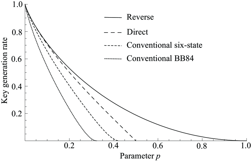
Figure 3.1: Comparison of the asymptotic key generation rates against the parameter $p$ of the amplitude damping channel (see Eq. (3.50)). “Reverse” and “Direct” are the asymptotic key generation rates when we use the reverse reconciliation and the direct reconciliation with our channel estimation procedure (Eqs. (3.52) and (3.51)) respectively. “Conventional six-state” and “Conventional BB84” are the asymptotic key generation rates of the six-state protocol and the BB84 protocol with the conventional channel estimation procedure. Note that the protocols with the conventional channel estimation procedure involves the noisy preprocessing [RGK05, KGR05] in the postprocessing.

Remark 3.6.1

As is mentioned in Remark 3.4.6, there is a possibility to improve the asymptotic key generation rate in Eq. (3.12) by the noisy preprocessing. If a $\{ccq\}$-state $\rho_{XYE}$ derived from a Choi operator $\rho\in{\cal P}_{c}$ satisfies the condition below, we can show that the noisy preprocessing does not improve the asymptotic key generation rate.

We define a $\{ccq\}$-state

$$\rho_{XYE}=\sum_{x,y\in\mathbb{F}_{2}}P_{XY}(x,y)|x,y\rangle\langle x,y|\otimes\rho_{E}^{x,y}$$

to be degradable state (from Alice to Bob and Eve) if there exist states $\{\hat{\rho}_{E}^{y}\}_{y\in\mathbb{F}_{2}}$ satisfying

$$\sum_{y\in\mathbb{F}_{2}}P_{Y|X}(y|x)\hat{\rho}_{E}^{y}=\rho_{E}^{x}:=\sum_{y\in\mathbb{F}_{2}}P_{Y|X}(y|x)\rho_{E}^{x,y}$$

for any $x\in\mathbb{F}_{2}$. If a $\{ccq\}$-state $\rho_{XYE}$ derived from a Choi operator $\rho$ is degradable, then the asymptotic key generation rate in Eq. (3.12) is optimal, that is, it cannot be improved by the noisy preprocessing.

The above statement is proved as follows. Even if we know the Choi operator $\rho$ in advance, the asymptotic key generation rate of any postprocessing is upper bounded by the quantum intrinsic information

$$I_{\rho}(X;Y\downarrow E):=\inf I_{\rho}(X;Y|E^{\prime}),$$

where

$$I_{\rho}(X;Y|E^{\prime}):=H_{\rho}(XE)+H_{\rho}(YE)-H_{\rho}(XYE)-H_{\rho}(E)$$

is the quantum conditional mutual information, and the infimum is taken over all $\{ccq\}$-states $\rho_{XYE^{\prime}}=(\mathrm{id}\otimes\mathcal{N}_{E\to E^{\prime}})(\rho_{XYE})$ for CPTP maps $\mathcal{N}_{E\to E^{\prime}}$ from system $E$ to $E^{\prime}$ [CEH⁺07]. Taking the identity map $\mathrm{id}_{E}$, the quantum conditional mutual information $I_{\rho}(X;Y|E)$ itself is an upper bound on the asymptotic key generation rate for any postprocessing.

Since we are now considering the postprocessing in which only Alice sends the public message, the maximum of the asymptotic key generation rate only depends on the distribution $P_{XY}$ and $\{cq\}$-state $\rho_{XE}$. Thus the maximum of the asymptotic key generation rate for $\rho_{XYE}$ is equals to that for degraded version of it,

$$\hat{\rho}_{XYE}:=\sum_{x,y}P_{XY}(x,y)|x\rangle\langle x|\otimes|y\rangle\langle y|\otimes\hat{\rho}_{E}^{y}.$$

Applying the above upper bound $I_{\rho}(X;Y|E)$ for the degraded $\{ccq\}$-state $\hat{\rho}_{XYE}$, the maximum of the asymptotic key generation rate is upper bounded by

$$I_{\hat{\rho}}(X;Y|E)$$

$$= I_{\hat{\rho}}(X;YE)-I_{\hat{\rho}}(X;E)$$

$$= H_{\hat{\rho}}(X|E)-H(X|Y)+I_{\hat{\rho}}(X;E|Y)$$

$$= H_{\rho}(X|E)-H(X|Y),$$

which is the desired upper bound, and equals to Eq. (3.12).

For the amplitude damping channel, we can show that the $\{ccq\}$-state $\rho_{XYE}$ is degradable by a straightforward calculation. Therefore, the asymptotic key generation rate in Eq. (3.12) is optimal for the amplitude damping channel.

Although we exclusively considered a key generated from the bit sequences transmitted and received by the $\mathsf{z}$-basis, we can also obtain a key from the bit sequences transmitted and received by the $\mathsf{x}$-basis (or the $\mathsf{y}$-basis for the six-state protocol). In this case, the asymptotic key generation rates are also given by Eqs. (3.12), (3.13), (3.15), and (3.16), where the definition of the $\{cq\}$-state $\rho_{XE}$ and the distribution $P_{XY}$ must be replaced appropriately.

For the amplitude damping channel, the asymptotic key generation rates for the forward and the reverse reconciliations can be written as functions of the parameter $p$:

$$1+h\left(\frac{1+\sqrt{1-p+p^{2}}}{2}\right)-h\left(\frac{p}{2}\right)-h\left(\frac{1+\sqrt{1-p}}{2}\right),$$ (3.53)

and

$$1-h\left(\frac{p}{2}\right)$$ (3.54)

respectively. They are plotted in Fig. 3.2, and compared to the asymptotic key generation rates with the conventional channel estimation.

From Fig. 3.2, we find that the asymptotic key generation rate with the reverse reconciliation is higher than that with the forward reconciliation. Although the difference between the asymptotic key generation rate with the forward and the reverse reconciliations comes from the difference between $H_{\rho}(X|Y)$ and $H_{\rho}(Y|X)$ in the case of the $\mathsf{z}$-basis, the difference between the asymptotic key generation rate with the forward and the reverse reconciliations comes from the difference between $H_{\rho}(X|E)$ and $H_{\rho}(Y|E)$, because $H_{\rho}(X|Y)=H_{\rho}(Y|X)$ in the case of the $\mathsf{x}$-basis.

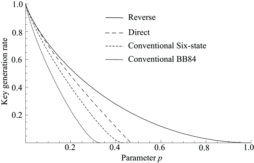
Figure 3.2: Comparison of the asymptotic key generation rates against the parameter $p$ of the amplitude damping channel (see Eq. (3.50)) for a key generated from the bit sequences transmitted and received by the $\mathsf{x}$-basis. “Reverse” and “Direct” are the asymptotic key generation rates when we use the reverse reconciliation and the direct reconciliation with our channel estimation procedure (Eqs. (3.54) and (3.53)) respectively. “Conventional six-state” and “Conventional BB84” are the asymptotic key generation rates of the six-state protocol and the BB84 protocol with the conventional channel estimation procedure. Note that the protocols with the conventional channel estimation procedure involves the noisy preprocessing [RGK05, KGR05] in the postprocessing.

3.6.2 Unital Channel and Rotation Channel

A channel is called a unital channel if ${\cal E}_{B}$ maps the completely mixed state $I/2$ to itself, or equivalently the corresponding Choi operator $\rho\in{\cal P}_{c}$ satisfies $\mathrm{Tr}_{A}[\rho]=I/2$. In the Stokes parameterization, a unital channel $(R,t)$ satisfies that $t$ is the zero vector. The unital channel has the following physical meaning in QKD protocols. When Eve conducts the Pauli cloning [Cer00] with respect to an orthonormal basis that is a rotated version of $\{|0_{\mathsf{z}}\rangle$, $|1_{\mathsf{z}}\rangle\}$, the quantum channel from Alice to Bob is not a Pauli channel but a unital channel. It is natural to assume that Eve cannot determine the direction of the basis $\{|0_{\mathsf{z}}\rangle$, $|1_{\mathsf{z}}\rangle\}$ accurately, and the unital channel deserve consideration in the QKD research as well as the Pauli channel.

By the singular value decomposition, we can decompose the matrix $R$ of the Stokes parameterization as

$$O_{2}\left[\begin{array}[]{ccc}e_{\mathsf{z}}&0&0\\ 0&e_{\mathsf{x}}&0\\ 0&0&e_{\mathsf{y}}\end{array}\right]O_{1},$$ (3.58)

where $O_{1}$ and $O_{2}$ are some rotation matrices, and $|e_{\mathsf{z}}|$, $|e_{\mathsf{x}}|$, and $|e_{\mathsf{y}}|$ are the singular value of the matrix $R$. Thus, we can consider the unital channel as a composition of a unitary channel, a Pauli channel

$$\rho\mapsto q_{\mathsf{i}}\rho+q_{\mathsf{z}}\sigma_{\mathsf{z}}\rho\sigma_{\mathsf{z}}+q_{\mathsf{x}}\sigma_{\mathsf{x}}\rho\sigma_{\mathsf{x}}+q_{\mathsf{y}}\sigma_{\mathsf{y}}\rho\sigma_{\mathsf{y}},$$

and a unitary channel [BW04], where

$$\begin{array}[]{rcl}q_{\mathsf{i}}&=&\frac{1+e_{\mathsf{z}}+e_{\mathsf{x}}+e_{\mathsf{y}}}{4},\\ q_{\mathsf{z}}&=&\frac{1+e_{\mathsf{z}}-e_{\mathsf{x}}-e_{\mathsf{y}}}{4},\\ q_{\mathsf{x}}&=&\frac{1-e_{\mathsf{z}}+e_{\mathsf{x}}-e_{\mathsf{y}}}{4},\\ q_{\mathsf{y}}&=&\frac{1-e_{\mathsf{z}}-e_{\mathsf{x}}+e_{\mathsf{y}}}{4}.\end{array}$$ (3.63)

For the six-state protocol, we can derive simple forms of $H_{\rho}(X|E)$ and $H_{\rho}(Y|E)$ as follows.

Lemma 3.6.2

For the unital channel, we have

$$H_{\rho}(X|E)=1-H[q_{\mathsf{i}},q_{\mathsf{z}},q_{\mathsf{x}},q_{\mathsf{y}}]+h\left(\frac{1+\sqrt{R_{\mathsf{zz}}^{2}+R_{\mathsf{xz}}^{2}+R_{\mathsf{yz}}^{2}}}{2}\right)$$ (3.64)

and

$$H_{\rho}(Y|E)=1-H[q_{\mathsf{i}},q_{\mathsf{z}},q_{\mathsf{x}},q_{\mathsf{y}}]+h\left(\frac{1+\sqrt{R_{\mathsf{zz}}^{2}+R_{\mathsf{zx}}^{2}+R_{\mathsf{zy}}^{2}}}{2}\right).$$ (3.65)

Proof.

We omit the proof because it can be proved in a similar manner as the latter half of the proof of Proposition 3.4.10. ∎

From this lemma, we can find that $R_{\mathsf{xz}}^{2}+R_{\mathsf{yz}}^{2}=R_{\mathsf{zx}}^{2}+R_{\mathsf{zy}}^{2}$ is the necessary and sufficient condition for $H_{\rho}(X|E)=H_{\rho}(Y|E)$. Furthermore, we can show $H_{\rho}(X|Y)=H_{\rho}(Y|X)=h((1+R_{\mathsf{zz}})/2)$ by a straightforward calculation.

For the BB84 protocol, ${\cal P}_{c}(\omega)$ consists of infinitely many elements in general. By using Proposition 3.4.10, we can calculate Eve’s worst case ambiguity as

$$\min_{\varrho\in{\cal P}_{c}(\omega)}H_{\varrho}(X|E)$$ (3.66)

$$= 1-h\left(\frac{1+d_{\mathsf{z}}}{2}\right)-h\left(\frac{1+d_{\mathsf{x}}}{2}\right)+h\left(\frac{1+\sqrt{R_{\mathsf{zz}}^{2}+R_{\mathsf{xz}}^{2}}}{2}\right)$$

and

$$\min_{\varrho\in{\cal P}_{c}(\omega)}H_{\varrho}(Y|E)$$ (3.67)

$$= 1-h\left(\frac{1+d_{\mathsf{z}}}{2}\right)-h\left(\frac{1+d_{\mathsf{x}}}{2}\right)+h\left(\frac{1+\sqrt{R_{\mathsf{zz}}^{2}+R_{\mathsf{zx}}^{2}}}{2}\right),$$

where $d_{\mathsf{z}}$ and $d_{\mathsf{x}}$ are the singular values of the matrix $\left[\begin{array}[]{cc}R_{\mathsf{zz}}&R_{\mathsf{zx}}\\ R_{\mathsf{xz}}&R_{\mathsf{xx}}\end{array}\right]$. From these formulae, we find that $R_{\mathsf{xz}}=R_{\mathsf{zx}}$ is the necessary and sufficient condition for $\min_{\varrho\in{\cal P}_{c}(\omega)}H_{\varrho}(X|E)$ coincides with $\min_{\varrho\in{\cal P}_{c}(\omega)}H_{\varrho}(Y|E)$. It should be noted that the singular values $(d_{\mathsf{z}},d_{\mathsf{x}})$ are different from the singular values $(|e_{\mathsf{z}}|,|e_{\mathsf{x}}|)$ in general because there exist off-diagonal elements $(R_{\mathsf{zy}},R_{\mathsf{xy}},R_{\mathsf{yz}},R_{\mathsf{yx}})$. By a straightforward calculation, we can show that $H_{\omega}(X|Y)=H_{\omega}(Y|X)=h((1+R_{\mathsf{zz}})/2)$.

In the rest of this section, we analyze a special class of the unital channel, the rotation channel, for the BB84 protocol. The rotation channel is a channel whose Stokes parameterization is given by

$$\left(\left[\begin{array}[]{ccc}\cos\vartheta&-\sin\vartheta&0\\ \sin\vartheta&\cos\vartheta&0\\ 0&0&1\end{array}\right],\left[\begin{array}[]{c}0\\ 0\\ 0\end{array}\right]\right).$$

The rotation channels occur, for example, when the directions of the transmitter and the receiver are not properly aligned.

For the rotation channel, Eq. (3.66) gives $\min_{\varrho\in{\cal P}_{c}(\omega)}H_{\varrho}(X|E)=1$, which implies that Eve gained no information. Thus, Eve’s worst case ambiguity, $\min_{\varrho\in{\cal P}_{c}(\omega)}H_{\varrho}(X|E)$ coincide with the true value $H_{\rho}(X|E)$, and the BB84 protocol can achieve the same asymptotic key generation rate as the six-state protocol.

The reason why we show this example is that Alice and Bob can share a secret key with a positive asymptotic key generation rate even though the so-called error rate is higher than the $25$% limit [GL03] in the BB84 protocol. The Bell diagonal entries of the Choi operator $\rho$ that corresponds to the rotation channel are $\cos^{2}(\vartheta/2)$, $0$, $0$, and $\sin^{2}(\vartheta/2)$. Thus the error rate is $\sin^{2}(\vartheta/2)$. For $\pi/3\leq\vartheta\leq 5\pi/3$, the error rate is higher than $25$%, but we can obtain the positive key rate, $1-h(\sin^{2}(\vartheta/2))$ except $\vartheta=\pi/2,3\pi/2$. Note that the asymptotic key generation rate in Eq. (3.39) is given by $1-2h(\sin^{2}(\vartheta/2))$. This fact verifies Curty et al’s suggestion [CLL04] that key agreement might be possible even for the error rates higher than $25$% limits.

3.7 Condition for Strict Improvement

So far, we have seen that the asymptotic key generation rates with our proposed channel estimation is at least as high as those with the conventional channel estimation (Section 3.5), and that the former is strictly higher than the latter for some specific channels (Section 3.6). For the BB84 protocol, the following theorems show the necessary and sufficient condition such that the former is strictly higher than the latter is that the channel is a Pauli channel.

Theorem 3.7.1

Suppose that $R_{\mathsf{zz}}\neq 0$ and $R_{\mathsf{xx}}\neq 0$. In the BB84 protocol, for the bit sequences transmitted and received by either $\mathsf{z}$-basis or the $\mathsf{x}$-basis, the asymptotic key generation rates with our proposed channel estimation are strictly higher than those with the conventional channel estimation if and only if $(t_{\mathsf{z}},t_{\mathsf{x}})\neq(0,0)$ or $(R_{\mathsf{zx}},R_{\mathsf{xz}})\neq(0,0)$.

Proof.

We only prove the statement for the direct reconciliation, because the statement for the reverse reconciliation can be proved in a similar manner.

“only if” part

Suppose that $(t_{\mathsf{z}},t_{\mathsf{x}})=(0,0)$ and $(R_{\mathsf{zx}},R_{\mathsf{xz}})=(0,0)$. Then, Propositions 3.4.10 and 3.5.6 implies that Eq. (3.15) is equal to Eq. (3.39). Similarly, the asymptotic key generation rate for the $\mathsf{x}$-basis with our proposed channel estimation is equal to that with the conventional channel estimation.

“if” part

Suppose that $t_{\mathsf{z}}\neq 0$. Let $\varrho^{*}$ be the Choi operator satisfying

$$H_{\varrho^{*}}(X|E)-H_{\varrho^{*}}(X|Y)=\min_{\varrho\in{\cal P}_{c}(\upsilon)}[H_{\varrho}(X|E)-H_{\varrho}(X|Y)].$$

Then, we have

$$H_{\varrho^{*}}(X|Y)=h\left(\frac{1+R_{\mathsf{zz}}}{2}\right)=H_{\omega}(W),$$

where $H_{\omega}(W)$ is the entropy of the distribution defined by

$$P_{W,\omega}(w):=\sum_{y\in\mathbb{F}_{2}}P_{XY,\omega}(y+w,y).$$

Then, $t_{\mathsf{z}}\neq 0$ and the arguments at the end of Remark 3.3.3 imply

$$H_{\omega}(X|Y)<H_{\omega}(W).$$

Since

$$\min_{\varrho\in{\cal P}_{c}(\omega)}H_{\varrho}(X|E)\geq\min_{\varrho\in{\cal P}_{c}(\upsilon)}H_{\varrho}(X|E)\geq H_{\varrho^{*}}(X|E),$$

Eq. (3.15) is strictly higher than Eq. (3.39). In a similar manner, we can show that the asymptotic key generation rate for the $\mathsf{x}$-basis with our proposed channel estimation is strictly higher that that with the conventional channel estimation if $t_{\mathsf{x}}\neq 0$.

Suppose that $(t_{\mathsf{z}},t_{\mathsf{x}})=(0,0)$ and $R_{\mathsf{zx}}\neq 0$. By using Proposition 3.4.10, we have

$$\min_{\varrho\in{\cal P}_{c}(\omega)}H_{\varrho}(X|E)-H_{\omega}(X|Y)$$ (3.69)

$$= 1-h\left(\frac{1+d_{\mathsf{z}}}{2}\right)-h\left(\frac{1+d_{\mathsf{x}}}{2}\right)$$

$$~{}~{}~{}~{}+h\left(\frac{1+\sqrt{R_{\mathsf{zz}}^{2}+R_{\mathsf{xz}}^{2}}}{2}\right)-h\left(\frac{1+R_{\mathsf{zz}}}{2}\right).$$

By the singular value decomposition, we have

$$\left[\begin{array}[]{cc}R_{\mathsf{zz}}&R_{\mathsf{zx}}\\ R_{\mathsf{xz}}&R_{\mathsf{xx}}\end{array}\right] = B~{}\mbox{diag}[d_{\mathsf{z}},d_{\mathsf{x}}]~{}A$$

$$= \left[\begin{array}[]{c}\langle B_{\mathsf{z}}|\\ \langle B_{\mathsf{x}}|\end{array}\right]\left[\begin{array}[]{cc}d_{\mathsf{z}}&0\\ 0&d_{\mathsf{x}}\end{array}\right]\left[\begin{array}[]{cc}|A_{\mathsf{z}}\rangle&|A_{\mathsf{x}}\rangle\end{array}\right]$$

$$= \left[\begin{array}[]{cc}\langle B_{\mathsf{z}}|\tilde{A}_{\mathsf{z}}\rangle&\langle B_{\mathsf{z}}|\tilde{A}_{\mathsf{x}}\rangle\\ \langle B_{\mathsf{x}}|\tilde{A}_{\mathsf{z}}\rangle&\langle B_{\mathsf{x}}|\tilde{A}_{\mathsf{x}}\rangle\end{array}\right],$$

where $A$ and $B$ are the rotation matrices, and we set $\langle\tilde{A}_{\mathsf{z}}|=(d_{\mathsf{z}}A_{\mathsf{zz}},d_{\mathsf{x}}A_{\mathsf{zx}})$ and $\langle\tilde{A}_{\mathsf{x}}|=(d_{\mathsf{z}}A_{\mathsf{xz}},d_{\mathsf{x}}A_{\mathsf{xx}})$. From Proposition 3.5.6, we have

$$\min_{\varrho\in{\cal P}_{c}(\upsilon)}[H_{\varrho}(X|E)-H_{\varrho}(X|Y)]$$ (3.73)

$$= 1-h\left(\frac{1+\langle B_{\mathsf{z}}|\tilde{A}_{\mathsf{z}}\rangle}{2}\right)-h\left(\frac{1+\langle B_{\mathsf{x}}|\tilde{A}_{\mathsf{x}}\rangle}{2}\right).$$

Subtracting Eq. (3.73) from Eq. (3.69), we have

$$h\left(\frac{1+\langle B_{\mathsf{x}}|\tilde{A}_{\mathsf{x}}\rangle}{2}\right)+h\left(\frac{1+\sqrt{R_{\mathsf{zz}}^{2}+R_{\mathsf{xz}}^{2}}}{2}\right)$$ (3.74)

$$~{}~{}-h\left(\frac{1+d_{\mathsf{z}}}{2}\right)-h\left(\frac{1+d_{\mathsf{x}}}{2}\right)$$

$$> h\left(\frac{1+\||\tilde{A}_{\mathsf{x}}\rangle\|}{2}\right)+h\left(\frac{1+\||\tilde{A}_{\mathsf{z}}\rangle\|}{2}\right)$$

$$~{}~{}-h\left(\frac{1+d_{\mathsf{z}}}{2}\right)-h\left(\frac{1+d_{\mathsf{x}}}{2}\right)$$

$$= h\left(\frac{1+\sqrt{d_{\mathsf{z}}^{2}A_{\mathsf{xz}}^{2}+d_{\mathsf{x}}A_{\mathsf{xx}}^{2}}}{2}\right)+h\left(\frac{1+\sqrt{d_{\mathsf{z}}^{2}A_{\mathsf{zz}}^{2}+d_{\mathsf{x}}^{2}A_{\mathsf{zx}}^{2}}}{2}\right)$$

$$~{}~{}-h\left(\frac{1+d_{\mathsf{z}}}{2}\right)-h\left(\frac{1+d_{\mathsf{x}}}{2}\right)$$

$$\geq A_{\mathsf{xz}}^{2}h\left(\frac{1+d_{\mathsf{z}}}{2}\right)+A_{\mathsf{xx}}^{2}h\left(\frac{1+d_{\mathsf{x}}}{2}\right)$$

$$~{}~{}+A_{\mathsf{zz}}^{2}h\left(\frac{1+d_{\mathsf{z}}}{2}\right)+A_{\mathsf{zx}}^{2}h\left(\frac{1+d_{\mathsf{x}}}{2}\right)$$

$$~{}~{}-h\left(\frac{1+d_{\mathsf{z}}}{2}\right)-h\left(\frac{1+d_{\mathsf{x}}}{2}\right)$$

$$= 0,$$

where the second inequality follows from the concavity of the function

$$h\left(\frac{1+\sqrt{x}}{2}\right),$$

which can be shown by a straight forward calculation. Thus, we have shown that Eq. (3.15) is strictly higher than Eq. (3.39). In a similar manner, we can show that the asymptotic key generation rate for the $\mathsf{x}$-basis with our proposed channel estimation is strictly higher that with the conventional channel estimation if $R_{\mathsf{xz}}\neq 0$. ∎

3.8 Summary

The results in this chapter is summarized as follows: In Section 3.2, we formally described the problem setting of the QKD protocols.

In Section 3.3, we showed the most basic IR procedure with one-way public communication. We introduced the condition such the IR procedure is universally correct (Definition 3.3.1). This condition was required because the IR procedure have to be robust against the fluctuation of the estimated probability of Alice and Bob’s bit sequences. We also explained the conventionally used IR procedure with the error correcting code, and we clarified that the length of the syndrome that must be transmitted in the conventional IR procedure is larger than that in our IR procedure (Remark 3.3.3). We showed how to apply the LDPC code with the sum product algorithm in our IR procedure (Remark 3.3.4).

In Section 3.4.1, we showed our proposed channel estimation procedure. We clarified a sufficient condition on the key generation rate such that Alice and Bob can share a secure key (Theorem 3.4.3), and we derived the asymptotic key generation rate formulae. We developed some techniques to calculate the asymptotic key generation rates (Propositions 3.4.9 and 3.4.10) for the BB84 protocol.

In Section 3.5, we explained the conventional estimation procedure. Then, we derived the asymptotic key generation rate formulae with the conventional channel estimation.

In Section 3.6, we investigated the asymptotic key generation rates for some examples of channels. We also introduced the concept of the degradable state, and we clarified that the asymptotic key generation rate in Eq. (3.12) is optimal if the state shared by Alice, Bob, and Eve is degradable (Remark 3.6.1). For the rotation channel, we clarified that the asymptotic key generation rate can be positive even if the error rate is higher than the 25% limit (Section 3.6.2).

Finally in Section 3.7, for the BB84 protocol we clarified the necessary and sufficient condition such that the asymptotic key generation rates with our proposed channel estimation is strictly higher than those with the conventional channel estimation is that the channel is a Pauli channel.

Chapter 4 Postprocessing

4.1 Background

The postprocessing shown in Chapter 3 consists of the IR procedure and the PA procedure. Roughly speaking, Alice and Bob can share a secret key with the key generation rate

$$H_{\rho}(X|E)-H_{\rho}(X|Y)$$ (4.1)

in that postprocessing. An interpretation of Eq. (4.1) is that the key generation rate is given by the difference between Eve’s ambiguity about Alice’s bit sequence subtracted by Bob’s ambiguity about Alice’s bit sequence. Therefore, when Eve’s ambiguity about Alice’s bit sequence is smaller than Bob’s ambiguity about Alice’s bit sequence, the key generation rate of that postprocessing is $0$.

In [Mau93], Maurer proposed a procedure, the so-called advantage distillation. The advantage distillation is conducted before the IR procedure, and the resulting postprocessing can have positive key generation rate even though Eq. (4.1) is negative. Gottesman and Lo applied the advantage distillation to the QKD protocols [GL03]. In the QKD protocols, the postprocessing with the advantage distillation was extensively studied by Bae and Acín [BA07].

In this chapter, we propose a new kind of postprocessing, which can be regarded as a generalization of the postprocessing that consists of the advantage distillation, the IR procedure, and the PA procedure. In our proposed postprocessing, the advantage distillation and the IR procedure are combined into one procedure, the two-way IR procedure. After the two-way IR procedure, we conduct the standard PA procedure.

The rest of this chapter is organized as follows: In Section 4.2, we review the advantage distillation. Then in Section 4.3, we propose the two-way information reconciliation procedure. In Section 4.4, we show a sufficient condition of the key generation rate such that Alice and Bob can share a secure key by our proposed postprocessing. In Section 4.5, we clarify that the key generation rate of our proposed postprocessing is higher than the other postprocessing by showing examples. Finally, we mention the relation between our proposed postprocessing and the entanglement distillation protocols in Section 4.6.

4.2 Advantage Distillation

In order to clarify the relation between the two-way IR procedure and the advantage distillation proposed by Maurer [Mau93], we review the postprocessing with the advantage distillation in this section. For convenience, the notations are adapted to this thesis. We assume that Alice and Bob have correlated binary sequences $\mathbf{x},\mathbf{y}\in\mathbb{F}_{2}^{2n}$ of even length. The pair of sequences $(\mathbf{x},\mathbf{y})$ is independently identically distributed (i.i.d.) according to a joint probability distribution $P_{XY}\in{\cal P}(\mathbb{F}_{2}\times\mathbb{F}_{2})$.

First, we need to define some auxiliary random variables to describe the postprocessing with the advantage distillation procedure. Let $\xi:\mathbb{F}_{2}^{2}\to\mathbb{F}_{2}$ be a function defined as $\xi(a_{1},a_{2}):=a_{1}+a_{2}$ for $a_{1},a_{2}\in\mathbb{F}_{2}$, and let $\zeta:\mathbb{F}_{2}^{2}\to\mathbb{F}_{2}$ be a function defined as $\zeta(a,0):=a$ and $\zeta(a,1):=0$ for $a\in\mathbb{F}_{2}$. For a pair of joint random variables $((X_{1},Y_{1})$, $(X_{2},Y_{2}))$ with a distribution, $P_{XY}^{2}$, we define random variables $U_{1}:=\xi(X_{1},X_{2})$, $V_{1}:=\xi(Y_{1},Y_{2})$ and $W_{1}:=U_{1}+V_{1}$. Furthermore, define random variables $U_{2}:=\zeta(X_{2},W_{1})$, $V_{2}:=\zeta(Y_{2},W_{1})$ and $W_{2}:=U_{2}+V_{2}$. For the pair of sequences, $\mathbf{x}=(x_{11},x_{12},\ldots,x_{n1},x_{n2})$ and $\mathbf{y}=(y_{11},y_{12},\ldots,y_{n1},y_{n2})$, which is distributed according to $P_{XY}^{2n}$, let $\mathbf{u}$, $\mathbf{v}$ and $\mathbf{w}$ be $2n$-bit sequences such that

$$u_{i1}:=\xi(x_{i1},x_{i2}),~{}~{}v_{i1}:=\xi(y_{i1},y_{i2}),~{}~{}w_{i1}:=u_{i1}+v_{i1}$$

and

$$u_{i2}:=\zeta(x_{i2},w_{i1}),~{}~{}v_{i2}:=\zeta(y_{i2},w_{i1}),~{}~{}w_{i2}:=u_{i2}+v_{i2}$$

for $1\leq i\leq n$. Then, the pair $(\mathbf{u},\mathbf{v})$ and the discrepancy, $\mathbf{w}$ between $\mathbf{u}$ and $\mathbf{v}$ are distributed according to the distribution $P_{U_{1}U_{2}V_{1}V_{2}W_{1}W_{2}}^{n}$.

The purpose of the advantage distillation is to classify blocks of length $2$ according to the parity $w_{i1}$ of the discrepancies in each block. When $P_{XY}$ is a distribution such that $P_{X}$ is the uniform distribution and $P_{Y|X}$ is a binary symmetric channel (BSC), the validity of this classification can be understood because we have

$$H(X_{i2}|Y_{i1}Y_{i2},W_{i}=1)=1.$$

This formula means that Alice have to send $X_{i2}$ itself if she want to tell Bob $X_{i2}$. Therefore, they cannot obtain any secret key from $X_{i2}$, and they should discard $X_{i2}$ if $W_{i}=1$. For general $P_{XY}$, the validity of above mentioned classification is unclear. For this reason, we employ a function which is more general than $\zeta$ in the next section.

By using above preparations, we can describe the postprocessing with the advantage distillation as follows. First, Alice sends the parity sequence $\mathbf{u}_{1}:=(u_{11},\ldots,u_{n1})$ to Bob so that he can identify the parity sequence $\mathbf{w}_{1}:=(w_{11},\ldots,w_{n1})$ of the discrepancies. Bob sends $\mathbf{w}_{1}$ back to Alice. Then, they discard $\mathbf{u}_{1}$ and $\mathbf{v}_{1}:=(v_{11},\ldots,v_{n1})$ respectively, because $\mathbf{u}_{1}$ is revealed to Eve. As the final step of the advantage distillation, Alice calculate the sequence $\mathbf{u}_{2}:=(u_{12},\ldots,u_{n2})$ by using $\mathbf{x}$ and $\mathbf{w}_{1}$.

At the end of the advantage distillation, Alice has $\mathbf{u}_{2}$ and Bob has $\mathbf{y}$ and $\mathbf{w}_{1}$ as a seed for the key agreement. By conducting the (one-way) IR procedure and the PA procedure for $(\mathbf{u}_{2},(\mathbf{y},\mathbf{w}_{1}))$, Alice and Bob share a secret key.

4.3 Two-Way Information Reconciliation

In this section, we show the two-way IR procedure. The essential difference between the two-way IR procedure and the advantage distillation is that Alice does not send the sequence $\mathbf{u}_{1}$ itself. As is usual in information theory, if we allow negligible error probability, Alice does not need to send the parity sequence, $\mathbf{u}_{1}$, to Bob to identify parity sequence $\mathbf{u}_{1}$. More precisely, Bob can decode $\mathbf{u}_{1}$ with negligible decoding error probability if Alice sends a syndrome with a sufficient length. Since Eve’s available information from the syndrome is much smaller than that from sequence $\mathbf{u}_{1}$ itself, Alice and Bob can use $\mathbf{u}_{1}$ as a seed for the key agreement.

First, we need to define some auxiliary random variables. As we have mentioned in the previous section, we use a function which is more general than $\zeta$. Let $\chi_{A},\chi_{B}$ be arbitrary functions from $\mathbb{F}_{2}^{2}$ to $\mathbb{F}_{2}$. Then, let $\zeta_{A}:\mathbb{F}_{2}^{3}\to\mathbb{F}_{2}$ be a function defined as $\zeta_{A}(a_{1},a_{2},a_{3}):=a_{1}$ if $\chi_{A}(a_{2},a_{3})=0$, and $\zeta_{A}(a_{1},a_{2},a_{3}):=0$ else. Let $\zeta_{B}:\mathbb{F}_{2}^{3}\to\mathbb{F}_{2}$ be a function defined as $\zeta_{B}(b_{1},b_{2},b_{3}):=b_{1}$ if $\chi_{B}(b_{2},b_{3})=0$, and $\zeta_{B}(b_{1},b_{2},b_{3}):=0$ else. By using these functions and the function $\xi$ defined in the previous section, we define the auxiliary random variables: $U_{1}:=\xi(X_{1},X_{2})$, $V_{1}:=\xi(Y_{1},Y_{2})$, $W_{1}:=U_{1}+V_{1}$, $U_{2}:=\zeta_{A}(X_{2},U_{1},V_{1})$, and $V_{2}:=\zeta_{B}(Y_{2},U_{1},V_{1})$. These auxiliary random variables mean that either Alice or Bob’s second bits are kept or discarded depending on the values of $\chi_{A}(U_{1},V_{1})$ and $\chi_{B}(U_{1},V_{1})$. The specific form of $\chi_{A}$ and $\chi_{B}$ will be given in Section 4.5 so that the asymptotic key generation rates are maximized.

Our proposed two-way IR procedure is conducted as follows:

1. Alice calculate $\mathbf{u}_{1}$ and Bob does the same for $\mathbf{v}_{1}$.

2. Alice calculates syndrome $t_{1}=t_{1}(\mathbf{u}_{1}):=M_{1}\mathbf{u}_{1}$, and sends it to Bob over the public channel.

3. Bob decodes $(\mathbf{y},t_{1})$ into estimate of $\mathbf{u}_{1}$ by a decoder $\hat{\mathbf{u}}_{1}:(\mathbb{F}_{2}^{2})^{n}\times\mathbb{F}_{2}^{k_{1}}\to\mathbb{F}_{2}^{n}$. Then, he calculates $\hat{\mathbf{w}}_{1}=\hat{\mathbf{u}}_{1}+\mathbf{v}_{1}$, and sends it to Alice over the public channel.

4. Alice calculates $\tilde{\mathbf{u}}_{2}$ by using $\mathbf{x}$, $\hat{\mathbf{w}}_{1}$, and the function $\zeta_{A}$. Bob also calculates $\tilde{\mathbf{v}}_{2}$ by using $\mathbf{y}$, $\hat{\mathbf{w}}$, and the function $\zeta_{B}$.

5. Alice calculates syndrome $\tilde{t}_{A,2}:=M_{A,2}\tilde{\mathbf{u}}_{2}$, and sends it to Bob over the public channel. Bob also calculate syndrome $\tilde{t}_{B,2}:=M_{B,2}\tilde{\mathbf{v}}_{2}$, and sends it to Alice over the public channel.

6. Bob decodes $(\mathbf{y},\hat{\mathbf{w}}_{1},\tilde{t}_{A,2})$ into estimate of $\mathbf{u}_{2}$ by using a decoder $\hat{\mathbf{u}}_{2}:(\mathbb{F}_{2}^{2})^{n}\times\mathbb{F}_{2}^{n}\times\mathbb{F}_{2}^{k_{A,2}}\to\mathbb{F}_{2}^{n}$. Alice also decodes $(\mathbf{x},\hat{\mathbf{w}}_{1},\tilde{t}_{B,2})$ by using a decoder $\hat{\mathbf{v}}_{2}:(\mathbb{F}_{2}^{2})^{n}\times\mathbb{F}_{2}^{n}\times\mathbb{F}_{2}^{k_{B,2}}\to\mathbb{F}_{2}^{n}$.

As we mentioned in Section 3.3, the decoding error probability of the two-way IR procedure have to be universally small for any distribution in the candidate $\{P_{XY,\theta}:~{}\theta\in\Theta\}$ that are estimated by Alice and Bob. For this reason, we introduce the concept that a two-way IR procedure is $\delta$-universally-correct in a similar manner as in Definition 3.3.1:

Definition 4.3.1

We define a two-way IR procedure to be $\delta$-universally-correct for the class $\{P_{XY,\theta}:~{}\theta\in\Theta\}$ of probability distribution if

$$P_{XY,\theta}^{2n}(\{(\mathbf{x},\mathbf{y}):~{}(\mathbf{u}_{1},\tilde{\mathbf{u}}_{2},\hat{\mathbf{v}}_{2})\neq(\mathbf{u}_{1},\mathbf{u}_{2},\mathbf{v}_{2})\mbox{ or }$$

$$~{}~{}~{}~{}~{}~{}~{}~{}~{}~{}~{}~{}~{}~{}~{}(\hat{\mathbf{u}}_{1},\hat{\mathbf{u}}_{2},\tilde{\mathbf{v}}_{2})\neq(\mathbf{u}_{1},\mathbf{u}_{2},\mathbf{v}_{2})\})\leq\delta$$

for any $\theta\in\Theta$.

An example of a decoder that fulfils the universality is the minimum entropy decoder. For Step (iii), the minimum entropy decoder is defined by

$$\hat{\mathbf{u}}_{1}(\mathbf{y},t_{1}):=\mathop{\rm argmin}\limits_{\mathbf{u}_{1}\in\mathbb{F}_{2}^{n}:M_{1}\mathbf{u}_{1}=t_{1}}H(P_{\mathbf{u}_{1}\mathbf{y}}),$$

where $P_{\mathbf{u}_{1}\mathbf{y}}\in{\cal P}_{n}(\mathbb{F}_{2}^{3})$ is the joint type of the sequence

$$(\mathbf{u}_{1},\mathbf{y})=((u_{11},y_{11},y_{12}),\ldots,(u_{n1},y_{n1},y_{n2}))$$

of length $n$. For Step (vi), the minimum entropy decoder is defined by

$$\hat{\mathbf{u}}_{2}(\mathbf{y},\mathbf{w}_{1},t_{2}):=\mathop{\rm argmin}\limits_{\mathbf{u}_{2}\in\mathbb{F}_{2}^{n}:M_{A,2}\mathbf{u}_{2}=t_{A,2}}H(P_{\mathbf{u}_{2}\mathbf{w}_{1}\mathbf{y}}),$$

where $P_{\mathbf{u}_{2}\mathbf{w}_{1}\mathbf{y}}\in{\cal P}_{n}(\mathbb{F}_{2}^{4})$ is the joint type of the sequence

$$(\mathbf{u}_{2},\mathbf{w}_{1},\mathbf{y})=((u_{12},w_{11},y_{11},y_{12}),\ldots,(u_{n2},w_{n1},y_{n1},y_{n2}))$$

of length $n$. The minimum entropy decoder for $\hat{\mathbf{v}}_{2}$ is defined in a similar manner.

Theorem 4.3.2

[Csi82, Theorem 1] Let $r_{1}$, $r_{A,1}$, and $r_{A,2}$ be real numbers that satisfy

$$r_{1}>\min_{\theta\in\Theta}H(U_{1,\theta}|Y_{1,\theta}Y_{2,\theta}),$$

$$r_{A,2}>\min_{\theta\in\Theta}H(U_{2,\theta}|W_{1,\theta}Y_{1,\theta}Y_{2,\theta}),$$

and

$$r_{B,2}>\min_{\theta\in\Theta}H(V_{2,\theta}|W_{1,\theta}X_{1,\theta}X_{2,\theta}),$$

respectively, where $U_{1,\theta}=\xi(X_{1,\theta},X_{2,\theta})$, $W_{1,\theta}=U_{1,\theta}+\xi(Y_{1,\theta},Y_{2,\theta})$, and $U_{2,\theta}=\zeta(X_{2,\theta},W_{1,\theta})$ for the random variables $(X_{1,\theta},X_{2,\theta},Y_{1,\theta},Y_{2,\theta})$ that are distributed according to $P_{XY,\theta}^{2}$. Then, for every sufficiently large $n$, there exist a $k_{1}\times n$ parity check matrix $M_{1}$, a $k_{A,2}\times n$ parity check matrix $M_{A,2}$, and a $k_{B,2}\times n$ parity check matrix $M_{B,2}$ such that $\frac{k_{1}}{n}\leq r_{1}$, $\frac{k_{A,2}}{n}\leq r_{A,2}$, and $\frac{k_{B,2}}{n}\leq r_{B,2}$, and the decoding error probability by the minimum entropy decoding satisfies

$$P_{XY,\theta}^{2n}(\{(\mathbf{x},\mathbf{y}):~{}(\mathbf{u}_{1},\tilde{\mathbf{u}}_{2},\hat{\mathbf{v}}_{2})\neq(\mathbf{u}_{1},\mathbf{u}_{2},\mathbf{v}_{2})\mbox{ or }$$

$$~{}~{}~{}~{}~{}~{}~{}~{}~{}~{}~{}~{}(\hat{\mathbf{u}}_{1},\hat{\mathbf{u}}_{2},\tilde{\mathbf{v}}_{2})\neq(\mathbf{u}_{1},\mathbf{u}_{2},\mathbf{v}_{2})\})$$

$$\leq e^{-nE_{1}}+e^{-nE_{A,2}}+e^{-nE_{B,2}}$$

for any $\theta\in\Theta$, where $E_{1},E_{A,2},E_{B,2}>0$ are constants that do not depends on $n$.

4.4 Security and Asymptotic Key Generation Rate

4.4.1 Sufficient Condition on Key Generation Rate for Secure Key Agreement

In this section, we show how Alice and Bob decide the parameters of the postprocessing and share a secret key. Then, we show a sufficient condition on the parameters such that Alice and Bob can share a secure key. We employ almost the same notations as in Section 3.4.1.

Let us start with the six-state protocol. Instead of the conditional von Neumann entropy $H_{\rho}(X|E)$, the quantities

$$H_{\rho}(U_{1}U_{2}V_{2}|W_{1}E_{1}E_{2})=H(\rho_{U_{1}U_{2}V_{2}W_{1}E_{1}E_{2}})-H(\rho_{W_{1}E_{1}E_{2}})$$ (4.2)

and

$$H_{\rho}(U_{2}V_{2}|U_{1}W_{1}E_{1}E_{2})=H(\rho_{U_{1}U_{2}V_{2}W_{1}E_{1}E_{2}})-H(\rho_{U_{1}W_{1}E_{1}E_{2}})$$ (4.3)

play important roles in our postprocessing, where the von Neumann entropies are calculated with respect to the operator $\rho_{U_{1}U_{2}V_{2}W_{1}E_{1}E_{2}}$ derived from $\rho_{AB}^{\otimes 2}$ via the measurement and the functions $\xi,\zeta_{A},\zeta_{B}$. For the ML estimator $\hat{\rho}(\mathbf{z})$ of $\rho\in{\cal P}_{c}$, we set

$$\hat{H}_{\mathbf{z}}(U_{1}U_{2}V_{2}|W_{1}E_{1}E_{2}):=H_{\hat{\rho}(\mathbf{z})}(U_{1}U_{2}V_{2}|W_{1}E_{1}E_{2})$$

and

$$\hat{H}_{\mathbf{z}}(U_{2}V_{2}|U_{1}W_{1}E_{1}E_{2}):=H_{\hat{\rho}(\mathbf{z})}(U_{2}V_{2}|U_{1}W_{1}E_{1}E_{2}),$$

which are the ML estimators of the quantities in Eqs. (4.2) and (4.3) respectively.

For the BB84 protocol, we similarly set

$$\hat{H}_{\mathbf{z}}(U_{1}U_{2}V_{2}|W_{1}E_{1}E_{2}):=\min_{\varrho\in{\cal P}_{c}(\hat{\omega}(\mathbf{z}))}H_{\varrho}(U_{1}U_{2}V_{2}|W_{1}E_{1}E_{2})$$

and

$$\hat{H}_{\mathbf{z}}(U_{2}V_{2}|U_{1}W_{1}E_{1}E_{2}):=\min_{\varrho\in{\cal P}_{c}(\hat{\omega}(\mathbf{z}))}H_{\varrho}(U_{2}V_{2}|U_{1}W_{1}E_{1}E_{2})$$

respectively.

According to the sample bit sequence $\mathbf{z}$, Alice and Bob decide the rate $\frac{k_{1}(\mathbf{z})}{n}$, $\frac{k_{A,2}(\mathbf{z})}{n}$, and $\frac{k_{B,2}(\mathbf{z})}{n}$ of the parity check matrices used in the two-way IR procedure. Furthermore, they also decide the length $\ell(\mathbf{z})$ of the finally distilled key according to the sample bit sequence $\mathbf{z}$. Then, they conduct the postprocessing as follows.

1. Alice and Bob undertake the two-way IR procedure of Section 4.3, and they obtain $(\mathbf{u}_{1},\tilde{\mathbf{u}}_{2},\hat{\mathbf{v}}_{2})$ and $(\hat{\mathbf{u}}_{1},\hat{\mathbf{u}}_{2},\tilde{\mathbf{v}}_{2})$ respectively.

2. Alice and Bob carry out the PA procedure to distill a key pair $(s_{A},s_{B})$. First, Alice randomly chooses a hash function, $f:\mathbb{F}_{2}^{3n}\to\{0,1\}^{\ell(\mathbf{z})}$, from a family of two-universal hash functions, and sends the choice of $f$ to Bob over the public channel. Then, Alice’s distilled key is $s_{A}=f(\mathbf{u}_{1},\tilde{\mathbf{u}}_{2},\hat{\mathbf{v}}_{2})$ and Bob’s distilled key is $s_{B}=f(\hat{\mathbf{u}}_{1},\hat{\mathbf{u}}_{2},\tilde{\mathbf{v}}_{2})$ respectively.

The distilled key pair and Eve’s available information can be described by a $\{cccq\}$-state, $\rho_{S_{A}S_{B}C\mathbf{E}}^{\mathbf{z}}$, where classical system $C$ consists of random variables $T_{1}$, $\tilde{T}_{A,2}$, and $\tilde{T}_{B,2}$ that describe the syndromes transmitted in Steps (ii) and (v) of the two-way IR procedure and random variable $F$ that describe the choice of the function in the PA procedure. Then, the security of the distilled key pair is defined in the same way as in Section 3.4.1, i.e., the key pair is said to be $\varepsilon$-secure if Eq. (3.8) is satisfied.

The following theorem gives a sufficient condition on $k_{1}(\mathbf{z})$, $k_{A,2}(\mathbf{z})$, $k_{B,2}(\mathbf{z})$, and $\ell(\mathbf{z})$ such that the distilled key is secure.

Theorem 4.4.1

For each sample sequence $\mathbf{z}\in{\cal Q}$, assume that the IR procedure is $\delta$-universally-correct for the class of distributions

$$\{P_{XY,\rho}:~{}\|\hat{\rho}(\mathbf{z})-\rho\|\leq\alpha\}$$

in the six-state protocol, and for the class of distributions

$$\{P_{XY,\omega}:~{}\|\hat{\omega}(\mathbf{z})-\omega\|\leq\alpha\}$$

in the BB84 protocol. For each $\mathbf{z}\in{\cal Q}$, if we set

$$\frac{\ell(\mathbf{z})}{2n}$$ (4.4)

$$< \frac{1}{2}\max\left[\hat{H}_{\mathbf{z}}(U_{1}U_{2}V_{2}|W_{1}E_{1}E_{2})-\eta(\alpha)-\frac{k_{1}(\mathbf{z})}{n}-\frac{k_{A,2}(\mathbf{z})}{n}-\frac{k_{B,2}(\mathbf{z})}{n},\right.$$

$$~{}~{}~{}~{}\left.\hat{H}_{\mathbf{z}}(U_{2}V_{2}|U_{1}W_{1}E_{1}E_{2})-\eta(\alpha)-\frac{k_{A,2}(\mathbf{z})}{n}-\frac{k_{B,2}(\mathbf{z})}{n}\right]-\nu_{n},$$

then the distilled key is $(\varepsilon+3\delta+\mu(\alpha,m))$-secure, where $\nu_{n}:=5\sqrt{\frac{\log(36/\varepsilon^{2})}{n}}+\frac{2\log(3/\varepsilon)}{n}$.

Proof.

We only prove the statement for the six-state protocol, because the statement for the BB84 protocol is proved exactly in the same way by replacing $\rho\in{\cal P}_{c}$ with $\omega\in\Omega$ and some other related quantities. The assertion of the theorem is proved by using Corollary 2.2.14, Lemma 2.2.10, Lemma 2.1.2, and Eq. (3.4).

For any $\rho\in{\cal P}_{c}$, Eq. (3.4) means that $\|\hat{\rho}(\mathbf{z})-\rho\|\leq\alpha$ with probability $1-\mu(\alpha,m)$. When $\|\hat{\rho}(\mathbf{z})-\rho\|>\alpha$, the distilled key pair is $1$-secure. For $\|\hat{\rho}(\mathbf{z})-\rho\|\leq\alpha$, we first assume (proved later) that the dummy key $S:=f(\mathbf{U}_{1},\mathbf{U}_{2},\mathbf{V}_{2})$ is $\varepsilon$-secret under the condition that Eve can access $(\mathbf{W}_{1},T_{1},T_{A,2},T_{B,2},F,\mathbf{E})$, i.e.,

$$\frac{1}{2}\|\rho^{\mathbf{z}}_{S\mathbf{W}_{1}T_{1}T_{A,2}T_{B,2}F\mathbf{E}}-\rho_{S}^{\mathbf{z},\mathrm{mix}}\otimes\rho^{\mathbf{z}}_{\mathbf{W}_{1}T_{1}T_{A,2}T_{B,2}F\mathbf{E}}\|\leq\varepsilon.$$ (4.5)

The assumption that the two-way IR procedure is $\delta$-universally-correct implies that $\hat{\mathbf{w}}_{1}=\mathbf{w}_{1}$, $\tilde{t}_{A,2}=t_{A,2}:=M_{A,2}\mathbf{u}_{2}$, and $\tilde{t}_{B,2}=t_{B,2}:=M_{B,2}\mathbf{v}_{2}$ with probability at least $1-\delta$. Since $(\mathbf{u}_{2},\tilde{\mathbf{u}}_{2})$, $(\mathbf{v}_{2},\hat{\mathbf{v}}_{2})$, $(\mathbf{w}_{1},\hat{\mathbf{w}}_{1})$, $(t_{A,2},\tilde{t}_{A,2})$, and $(t_{B,2},\tilde{t}_{B,2})$ can be computed from $(\mathbf{x},\mathbf{y})$, by using Lemma 2.1.2, we have

$$\|\rho^{\mathbf{z}}_{\mathbf{X}\mathbf{Y}\mathbf{U}_{1}\tilde{\mathbf{U}}_{2}\hat{\mathbf{V}}_{2}\hat{\mathbf{W}}_{1}T_{1}\tilde{T}_{A,2}\tilde{T}_{B,2}F\mathbf{E}}-\rho^{\mathbf{z}}_{\mathbf{X}\mathbf{Y}\mathbf{U}_{1}\mathbf{U}_{2}\mathbf{V}_{2}\mathbf{W}_{1}T_{1}T_{A,2}T_{B,2}F\mathbf{E}}\|\leq 2\delta.$$

Since the trace distance does not increase by CP maps, we have

$$\|\rho^{\mathbf{z}}_{S_{A}\mathbf{W}_{1}T_{1}\tilde{T}_{A,2}\tilde{T}_{B,2}F\mathbf{E}}-\rho^{\mathbf{z}}_{S\mathbf{W}_{1}T_{1}T_{A,2}T_{B,2}F\mathbf{E}}\|\leq 2\delta.$$

Therefore, the statement that the dummy key $S$ is $\varepsilon$-secret implies that the actual key $S_{A}$ is $(\varepsilon+2\delta)$-secret as follows:

$$\|\rho^{\mathbf{z}}_{S_{A}\hat{\mathbf{W}}_{1}T_{1}\tilde{T}_{A,2}\tilde{T}_{B,2}F\mathbf{E}}-\rho_{S_{A}}^{\mathbf{z},\mathrm{mix}}\otimes\rho^{\mathbf{z}}_{\hat{\mathbf{W}}_{1}T_{1}\tilde{T}_{2,A}\tilde{T}_{2,B}F\mathbf{E}}\|$$

$$\leq \|\rho^{\mathbf{z}}_{S_{A}\hat{\mathbf{W}}_{1}T_{1}\tilde{T}_{A,2}\tilde{T}_{B,2}F\mathbf{E}}-\rho^{\mathbf{z}}_{S\mathbf{W}_{1}T_{1}T_{A,2}T_{B,2}F\mathbf{E}}\|$$

$$+\|\rho^{\mathbf{z}}_{S\mathbf{W}_{1}T_{1}T_{A,2}T_{B,2}F\mathbf{E}}-\rho_{S}^{\mathbf{z},\mathrm{mix}}\otimes\rho^{\mathbf{z}}_{\mathbf{W}_{1}T_{1}T_{A,2}T_{B,2}F\mathbf{E}}\|$$

$$+\|\rho_{S}^{\mathbf{z},\mathrm{mix}}\otimes\rho^{\mathbf{z}}_{\mathbf{W}_{1}T_{1}T_{A,2}T_{B,2}F\mathbf{E}}-\rho_{S_{A}}^{\mathbf{z},\mathrm{mix}}\otimes\rho^{\mathbf{z}}_{\hat{\mathbf{W}}_{1}T_{1}\tilde{T}_{A,2}\tilde{T}_{B,2}F\mathbf{E}}\|,$$

where the first term is upper bounded by $2\delta$, the second term is upper bounded by $2\varepsilon$, and the third term is also upper bounded by $2\delta$ because $\rho_{S}^{\mathbf{z},\mathrm{mix}}=\rho_{S_{A}}^{\mathbf{z},\mathrm{mix}}$. The assumption that the two-way IR procedure is $\delta$-universally-correct also implies that the distilled key pair $(S_{A},S_{B})$ is $\delta$-universally-correct. Thus, the key pair is $(\varepsilon+3\delta)$-secure if $\|\hat{\rho}(\mathbf{z})-\rho\|\leq\alpha$. Averaging over the sample sequence $\mathbf{z}\in{\cal Q}$, the distilled key pair is $(\varepsilon+3\delta+\mu(\alpha,m))$-secure.

One thing we have left is to prove Eq. (4.5). According to Lemma 2.2.10, the inequality

$$\frac{\ell(\mathbf{z})}{2n}<$$

$$\frac{1}{2}\left[\hat{H}_{\mathbf{z}}(U_{1}U_{2}V_{2}|W_{1}E_{1}E_{2})-\eta(\alpha)-\frac{k_{1}(\mathbf{z})}{n}-\frac{k_{A,2}(\mathbf{z})}{n}-\frac{k_{B,2}(\mathbf{z})}{n}\right]-\nu_{n}$$

implies the inequality

$$\ell(\mathbf{z})<$$

$$H_{\min}^{\bar{\varepsilon}}(\rho_{\mathbf{U}_{1}\mathbf{U}_{2}\mathbf{V}_{2}\mathbf{W}_{1}\mathbf{E}}|\mathbf{W}_{1}\mathbf{E})-k_{1}(\mathbf{z})-k_{A,2}(\mathbf{z})-k_{B,2}(\mathbf{z})-2\log(3/2\varepsilon).$$

Thus, Corollary 2.2.14 implies that the dummy key $S$ is $\varepsilon$-secret.

Since the syndrome $T_{1}$ is computed from the sequence $\mathbf{U}_{1}$, if the dummy key $S$ is $\varepsilon$-secret in the case that Eve can access the sequence $\mathbf{U}_{1}$, then the dummy key $S$ must be $\varepsilon$-secret in the case that Eve can only access the syndrome $T_{1}$ instead of $\mathbf{U}_{1}$. According to Lemma 2.2.10, the inequality

$$\frac{\ell(\mathbf{z})}{2n}<\frac{1}{2}\left[\hat{H}_{\mathbf{z}}(U_{2}V_{2}|U_{1}W_{1}E_{1}E_{2})-\eta(\alpha)-\frac{k_{A,2}(\mathbf{z})}{n}-\frac{k_{B,2}(\mathbf{z})}{n}\right]-\nu_{n}$$

implies the inequality

$$\ell(\mathbf{z})<H_{\min}^{\bar{\varepsilon}}(\rho_{\mathbf{U}_{1}\mathbf{U}_{2}\mathbf{V}_{2}\mathbf{W}_{1}\mathbf{E}}|\mathbf{U}_{1}\mathbf{W}_{1}\mathbf{E})-k_{A,2}(\mathbf{z})-k_{B,2}(\mathbf{z})-2\log(3/2\varepsilon).$$

Thus, Corollary 2.2.14 implies that the dummy key $S$ is $\varepsilon$-secret.

Combining above two arguments, we have the assertion of the theorem. ∎

Remark 4.4.2

The maximization in Eq. (4.4) is very important. If either of them is omitted, the key generation rate of the postprocessing can be underestimated, as will be discussed in Section 4.5.

Remark 4.4.3

By switching the role of Alice and Bob, we obtain a postprocessing with the reverse two-way IR procedure. For the postprocessing with the reverse two-way IR procedure, we can show almost the same statement as Theorem 4.4.1 by replacing $U_{1}$ with $V_{1}$, and by using the $\delta$-universally-correct for the reverse two-way IR procedure.

4.4.2 Asymptotic Key Generation Rates

In this section, we derive the asymptotic key generation rate formula for the postprocessing with the two-way IR procedure. First, we consider the six-state protocol. Since the ML estimator is a consistent estimator, in a similar arguments as in Sections 3.4.1 and 3.4.3, we can set the sequence of the key generation rates so that it converges to the asymptotic key generation rate formula

$$\frac{1}{2}\max\left[H_{\rho}(U_{1}U_{2}V_{2}|W_{1}E_{1}E_{2})-H_{\rho}(U_{1}|Y_{1}Y_{2})\right.$$ (4.6)

$$~{}~{}~{}~{}~{}~{}~{}~{}~{}~{}~{}~{}~{}~{}~{}-H_{\rho}(U_{2}|W_{1}Y_{1}Y_{2})-H_{\rho}(V_{2}|W_{1}X_{1}X_{2}),$$

$$\left.H_{\rho}(U_{2}V_{2}|U_{1}W_{1}E_{1}E_{2})-H_{\rho}(U_{2}|W_{1}Y_{1}Y_{2})-H_{\rho}(V_{2}|W_{1}X_{1}X_{2})\right]$$

in probability as $m,n\to\infty$. We can also derive the asymptotic key generation formula for the postprocessing with the reverse two-way IR procedure as

$$\frac{1}{2}\max\left[H_{\rho}(V_{1}U_{2}V_{2}|W_{1}E_{1}E_{2})-H_{\rho}(V_{1}|X_{1}X_{2})\right.$$ (4.7)

$$~{}~{}~{}~{}~{}~{}~{}~{}~{}~{}~{}~{}~{}~{}~{}-H_{\rho}(U_{2}|W_{1}Y_{1}Y_{2})-H_{\rho}(V_{2}|W_{1}X_{1}X_{2}),$$

$$\left.H_{\rho}(U_{2}V_{2}|U_{1}W_{1}E_{1}E_{2})-H_{\rho}(U_{2}|W_{1}Y_{1}Y_{2})-H_{\rho}(V_{2}|W_{1}X_{1}X_{2})\right].$$

Next, we consider the BB84 protocol. Since the ML estimator is a consistent estimator, in a similar arguments as in Sections 3.4.1 and 3.4.4, we can set the sequence of the key generation rates so that it converges to the asymptotic key generation rate formula

$$\frac{1}{2}\min_{\varrho\in{\cal P}_{c}(\omega)}\max\left[H_{\varrho}(U_{1}U_{2}V_{2}|W_{1}E_{1}E_{2})-H_{\omega}(U_{1}|Y_{1}Y_{2})\right.$$ (4.8)

$$~{}~{}~{}~{}~{}~{}~{}~{}~{}~{}~{}~{}~{}~{}~{}-H_{\omega}(U_{2}|W_{1}Y_{1}Y_{2})-H_{\omega}(V_{2}|W_{1}X_{1}X_{2}),$$

$$\left.H_{\varrho}(U_{2}V_{2}|U_{1}W_{1}E_{1}E_{2})-H_{\omega}(U_{2}|W_{1}Y_{1}Y_{2})-H_{\omega}(V_{2}|W_{1}X_{1}X_{2})\right],$$

in probability as $m,n\to\infty$.

We can also derive the asymptotic key generation rate formula for the postprocessing with the reverse two-way IR procedure as

$$\frac{1}{2}\min_{\varrho\in{\cal P}_{c}(\omega)}\max\left[H_{\varrho}(V_{1}U_{2}V_{2}|W_{1}E_{1}E_{2})-H_{\omega}(U_{1}|X_{1}X_{2})\right.$$ (4.9)

$$~{}~{}~{}~{}~{}~{}~{}~{}~{}~{}~{}~{}~{}~{}~{}-H_{\omega}(U_{2}|W_{1}Y_{1}Y_{2})-H_{\omega}(V_{2}|W_{1}X_{1}X_{2}),$$

$$\left.H_{\varrho}(V_{2}|U_{1}W_{1}E_{1}E_{2})-H_{\omega}(U_{2}|W_{1}Y_{1}Y_{2})-H_{\omega}(V_{2}|W_{1}X_{1}X_{2})\right].$$

The following propositions are useful to calculate the minimizations in Eqs. (4.8) and (4.9).

Proposition 4.4.4

For two density operator $\rho^{1},\rho^{2}\in{\cal P}_{c}$ and a probabilistically mixture $\rho^{\prime}:=\lambda\rho^{1}+(1-\lambda)\rho^{2}$, Eve’s ambiguities are convex, i.e., we have

$$H_{\rho^{\prime}}(U_{1}U_{2}V_{2}|W_{1}E_{1}E_{2})$$

$$\leq \lambda H_{\rho^{1}}(U_{1}U_{2}V_{2}|W_{1}E_{1}E_{2})+(1-\lambda)H_{\rho^{2}}(U_{1}U_{2}V_{2}|W_{1}E_{1}E_{2})$$

and

$$H_{\rho^{\prime}}(U_{2}V_{2}|U_{1}W_{1}E_{1}E_{2})$$

$$\leq \lambda H_{\rho^{1}}(U_{2}V_{2}|U_{1}W_{1}E_{1}E_{2})+(1-\lambda)H_{\rho^{2}}(U_{2}V_{2}|U_{1}W_{1}E_{1}E_{2}),$$

where $\rho^{\prime}_{U_{1}U_{2}V_{2}W_{1}E_{1}E_{2}}$ is the density operator derived from a purification $(\psi^{\prime}_{ABE})^{\otimes 2}$ of $(\rho^{\prime}_{AB})^{\otimes 2}$.

Proof.

The statement of this proposition is shown exactly in the same way as Proposition 3.4.7. ∎

Proposition 4.4.5

For the BB84 protocol, the minimization in Eqs. (4.8) and (4.9) is achieved by Choi operator $\varrho$ whose components $R_{\mathsf{zy}}$, $R_{\mathsf{xy}}$, $R_{\mathsf{yz}}$, $R_{\mathsf{yx}}$, and $t_{\mathsf{y}}$, are all $0$.

Proof.

The statement of this proposition is shown exactly in the same way as Proposition 3.4.9 by using Proposition 4.4.4. ∎

Remark 4.4.6

By using the chain rule of von Neumann entropy, we can rewrite Eq. (4.6) as

$$\frac{1}{2}\{\max[H_{\rho}(U_{1}|W_{1}E_{1}E_{2})-H(U_{1,\rho}|Y_{1,\rho}Y_{2,\rho}),0]$$ (4.10)

$$+H_{\rho}(U_{2}V_{2}|U_{1}W_{1}E_{1}E_{2})-H_{\rho}(U_{2}|W_{1}Y_{1}Y_{2})-H_{\rho}(V_{2}|W_{1}X_{1}X_{2})\}.$$

We can interpret this formula as follows. If Bob’s ambiguity $H_{\rho}(U_{1}|Y_{1}Y_{2})$ about bit $U_{1}$ is smaller than Eve’s ambiguity $H_{\rho}(U_{1}|W_{1}E_{1}E_{2})$ about $U_{1}$, then Eve cannot decode sequence $\mathbf{U}_{1}$ [SW73, DW03], and there exists some remaining ambiguity about bit $U_{1}$ for Eve. We can thus distill some secure key from bit $U_{1}$. On the other hand, if Bob’s ambiguity $H_{\rho}(U_{1}|Y_{1}Y_{2})$ about bit $U_{1}$, i.e., the amount of transmitted syndrome per bit, is larger than Eve’s ambiguity $H_{\rho}(U_{1}|W_{1}E_{1}E_{2})$ about $U_{1}$, then Eve might be able to decode sequence $\mathbf{U}_{1}$ from her side information and the transmitted syndrome [SW73, DW03]. Thus, there exists the possibility that Eve can completely know bit $U_{1}$, and we can distill no secure key from bit $U_{1}$, because we have to consider the worst case in a cryptography scenario. Consequently, sending the compressed version (syndrome) of sequence $\mathbf{U}_{1}$ instead of $\mathbf{U}_{1}$ itself is not always effective, and the slope of the key rate curves change when Eve becomes able to decode $\mathbf{U}_{1}$ (see Figs. 4.1, 4.2, 4.3, 4.4, 4.5).

A similar argument also holds for the BB84 protocol.

Remark 4.4.7

If we take the functions $\chi_{A}$ and $\chi_{B}$ as

$$\chi_{A}(a_{1},a_{2}):=\left\{\begin{array}[]{ll}0&\mbox{if }a_{1}=a_{2}\\ 1&\mbox{else}\end{array}\right.$$ (4.13)

and

$$\chi_{B}(b_{1},b_{2})=1.$$ (4.14)

Then, the postprocessing proposed in this thesis reduces to the postprocessing proposed in [WMUK07].

Remark 4.4.8

The asymptotic key generation rate (for the six-state protocol) of the postprocessing with the advantage distillation is given by

$$\frac{1}{2}[H_{\rho}(U_{2}|U_{1}W_{1}E_{1}E_{2})-H_{\rho}(U_{2}|W_{1}Y_{1}Y_{2})],$$ (4.15)

where the auxiliary random variables $U_{1},U_{2},W_{1}$ are defined as in Section 4.2, or they are defined by using the functions $\chi_{A},\chi_{B}$ given in Eqs. (4.13) and (4.14). From Eqs. (4.6) and (4.15), we can find that the asymptotic key generation rate of the proposed postprocessing is at least as high as that of the postprocessing with the advantage distillation if we employ appropriate functions $\chi_{A},\chi_{B}$.

A similar argument also holds for the BB84 protocol.

Remark 4.4.9

In [GA08], Gohari and Anantharam proposed a two-way postprocessing which is similar to our proposed two-way postprocessing. They derived the asymptotic key generation rate formula of their proposed postprocessing. Although their postprocessing seems to be a generalization of our proposed postprocessing, the asymptotic key generation rate (Eq. (4.6)) of our proposed postprocessing cannot be derived by their asymptotic key generation rate formula. By modifying their formula for the QKD protocol, we can only derive the asymptotic key generation rate

$$\frac{1}{2}[H_{\rho}(U_{1}|E_{1}E_{2})-H_{\rho}(U_{1}|Y_{1}Y_{2})$$ (4.16)

$$+H_{\rho}(W_{1}|U_{1}E_{1}E_{2})-H_{\rho}(W_{1}|U_{1}X_{1}X_{2})$$

$$+H_{\rho}(U_{2}|U_{1}W_{1}E_{1}E_{2})-H_{\rho}(U_{2}|U_{1}W_{1}Y_{1}Y_{2})$$

$$+H_{\rho}(V_{2}|U_{1}W_{1}U_{2}E_{1}E_{2})-H_{\rho}(V_{2}|U_{1}W_{1}U_{2}X_{1}X_{2})].$$

For a Pauli channel, since $W_{1}$ is independent from $(X_{1},X_{2})$ and $H_{\rho}(W_{1}|E_{1}E_{2})=0$, Eq. (4.16) is strictly smaller than Eq. (4.6).

The underestimation of the asymptotic key generation rate comes from the following reason. In Gohari and Anantharam’s postprocessing, a syndrome of $\mathbf{w}_{1}$ is transmitted over the public channel, and the length of the syndrome is roughly $H_{\rho}(W_{1}|U_{1}X_{1}X_{2})$. When the syndrome is transmitted over the public channel, Eve cannot obtain more information than $\mathbf{w}_{1}$ itself. The lack of this observation results into Eq. (4.16).

4.5 Comparison of Asymptotic Key Generation Rates for Specific Channels

In this section, we compare the asymptotic key generation rates of the proposed postprocessing, the postprocessing with the advantage distillation, the one-way postprocessing for representative specific channels.

4.5.1 Pauli Channel

When the channel between Alice and Bob is a Pauli channel, the Stokes parameterization of the corresponding density operator $\rho\in{\cal P}_{c}$ is

$$\left(\left[\begin{array}[]{ccc}e_{\mathsf{z}}&0&0\\ 0&e_{\mathsf{x}}&0\\ 0&0&e_{\mathsf{y}}\end{array}\right],\left[\begin{array}[]{c}0\\ 0\\ 0\end{array}\right]\right),$$ (4.23)

for $-1\leq e_{\mathsf{z}},e_{\mathsf{x}},e_{\mathsf{y}}\leq 1$. The Choi operator of the Pauli channel is a Bell diagonal state:

$$\rho=\sum_{\mathsf{k},\mathsf{l}\in\mathbb{F}_{2}}P_{\mathsf{KL}}(\mathsf{k},\mathsf{l})|\psi(\mathsf{k},\mathsf{l})\rangle\langle\psi(\mathsf{k},\mathsf{l})|,$$ (4.24)

where $P_{\mathsf{KL}}$ is a distribution on $\mathbb{F}_{2}\times\mathbb{F}_{2}$ defined by

$$\begin{array}[]{rcl}P_{\mathsf{KL}}(0,0)&=&\frac{1+e_{\mathsf{z}}+e_{\mathsf{x}}+e_{\mathsf{y}}}{4},\\ P_{\mathsf{KL}}(0,1)&=&\frac{1+e_{\mathsf{z}}-e_{\mathsf{x}}-e_{\mathsf{y}}}{4},\\ P_{\mathsf{KL}}(1,0)&=&\frac{1-e_{\mathsf{z}}+e_{\mathsf{x}}-e_{\mathsf{y}}}{4},\\ P_{\mathsf{KL}}(1,1)&=&\frac{1-e_{\mathsf{z}}-e_{\mathsf{x}}+e_{\mathsf{y}}}{4},\end{array}$$ (4.29)

and

$$|\psi(0,0)\rangle := \frac{|00\rangle+|11\rangle}{\sqrt{2}},$$

$$|\psi(1,0)\rangle := \frac{|01\rangle+|10\rangle}{\sqrt{2}},$$

$$|\psi(0,1)\rangle := \frac{|00\rangle-|11\rangle}{\sqrt{2}},$$

$$|\psi(1,1)\rangle := \frac{|01\rangle-|10\rangle}{\sqrt{2}}.$$

We occasionally abbreviate $P_{\mathsf{KL}}(\mathsf{k},\mathsf{l})$ as $p_{\mathsf{kl}}$. Note that the Pauli channel is a special class of the unital channel discussed in Section 3.6.2.

The following lemma simplify the calculation of Eq. (4.8) for a Pauli channel.

Lemma 4.5.1

For a Bell diagonal Choi operator $\rho$, the minimizations in Eqs. (4.8) (4.9) are achieved by a Bell diagonal operator $\varrho\in{\cal P}_{c}(\omega)$.

Proof.

This lemma is a straightforward corollary of Proposition 4.4.4. ∎

Lemma 4.5.2

For Bell diagonal state $\rho$, the asymptotic key generation rate is maximized when we employ the functions $\chi_{A},\chi_{B}$ given by Eqs. (4.13) and (4.14).

Proof.

Since $H_{\rho}(X_{2}|W_{1}=1,Y_{1}Y_{2})=1$ and $H_{\rho}(X_{2}|W_{1}=1,E_{1}E_{2})\leq 1$, $X_{2}$ should be discarded if $W_{1}=1$. Similarly, $Y_{2}$ should be discarded if $W_{1}=0$. Since the Bell diagonal Choi operator is symmetric with respect to Alice and Bob’s subsystem, we have

$$H_{\rho}(X_{2}|W_{1}=0,U_{1}E_{1}E_{2})=H_{\rho}(Y_{2}|W_{1}=0,U_{1}E_{1}E_{2}),$$

and

$$H_{\rho}(X_{2}|W_{1}=0,Y_{1}Y_{2})=H_{\rho}(Y_{2}|W_{1}=0,X_{1}X_{2}).$$

Furthermore, we have

$$H_{\rho}(Y_{2}|W_{1}=0,U_{1}X_{2}E_{1}E_{2})\leq H_{\rho}(Y_{2}|W_{1}=0,X_{1}X_{2}).$$ (4.30)

Therefore, the functions given by Eqs. (4.13) and (4.14) are optimal. Note that Eq. (4.30) means that we should not keep $Y_{2}$ if we keep $X_{2}$. ∎

By Lemmas 4.5.1 and 4.5.2, it suffice to consider the functions given by Eqs. (4.13) and (4.14) if the channel is a Pauli channel. Therefore, we employ the functions given by Eqs. (4.13) and (4.14) throughout this subsection. Furthermore, we can find that the asymptotic key generation rates for the direct and the reverse IR procedure coincide, because $H_{\rho}(U_{1}|W_{1}E_{1}E_{2})=H_{\rho}(V_{1}|W_{1}E_{1}E_{2})$ and $H_{\rho}(U_{1}|Y_{1}Y_{2})=H_{\rho}(V_{1}|X_{1}X_{2})$. Therefore, we only consider the asymptotic key generation rate for the direct IR procedure throughout this subsection.

Theorem 4.5.3

For a Bell diagonal state $\rho$, we have

$$\frac{1}{2}\max\left[H_{\rho}(U_{1}U_{2}|W_{1}E_{1}E_{2})-H_{\rho}(U_{1}|Y_{1}Y_{2})\right.$$ (4.31)

$$~{}~{}~{}~{}~{}~{}~{}~{}~{}~{}~{}~{}~{}~{}~{}-H_{\rho}(U_{2}|W_{1}Y_{1}Y_{2}),$$

$$~{}~{}~{}~{}~{}~{}~{}~{}~{}~{}\left.H_{\rho}(U_{2}|U_{1}W_{1}E_{1}E_{2})-H_{\rho}(U_{2}|W_{1}Y_{1}Y_{2})\right],$$

$$= \max[1-H(P_{\mathsf{KL}})$$

$$+\frac{P_{\bar{\mathsf{K}}}(1)}{2}h\left(\frac{p_{00}p_{10}+p_{01}p_{11}}{(p_{00}+p_{01})(p_{10}+p_{11})}\right),$$

$$\hskip 28.45274pt\frac{P_{\bar{\mathsf{K}}}(0)}{2}(1-H(P_{\mathsf{KL}}^{\prime}))],$$

where

$$P_{\bar{\mathsf{K}}}(0) := (p_{00}+p_{01})^{2}+(p_{10}+p_{11})^{2},$$

$$P_{\bar{\mathsf{K}}}(1) := 2(p_{00}+p_{01})(p_{10}+p_{11}),$$

and

$$P_{\mathsf{KL}}^{\prime}(0,0) := \frac{p_{00}^{2}+p_{01}^{2}}{(p_{00}+p_{01})^{2}+(p_{10}+p_{11})^{2}},$$

$$P_{\mathsf{KL}}^{\prime}(1,0) := \frac{2p_{00}p_{01}}{(p_{00}+p_{01})^{2}+(p_{10}+p_{11})^{2}},$$

$$P_{\mathsf{KL}}^{\prime}(0,1) := \frac{p_{10}^{2}+p_{11}^{2}}{(p_{00}+p_{01})^{2}+(p_{10}+p_{11})^{2}},$$

$$P_{\mathsf{KL}}^{\prime}(1,1) := \frac{2p_{10}p_{11}}{(p_{00}+p_{01})^{2}+(p_{10}+p_{11})^{2}}.$$

The theorem is proved by a straightforward calculation, and the proof is presented at the end of this section.

Combining Lemma 4.5.1, Theorem 4.5.3, and Eq (4.29), it is straightforward to calculate the asymptotic key generation rate for a Pauli channel. As a special case of the Pauli channel, we consider the depolarizing channel. The depolarizing channel is parameterized by one real parameter $e\in[0,1/2]$, and the Bell diagonal entries of the Choi operator are given by $p_{00}=1-3e/2$, $p_{10}=p_{01}=p_{11}=e/2$. For the six-state protocol, it is straightforward to calculate the asymptotic key generation rate, which is plotted in Fig. 4.1. According to Lemma 4.5.1, it is sufficient to take the minimization over the subset ${\cal P}_{c,\mathrm{Bell}}(\omega)\subset{\cal P}_{c}(\omega)$ that consists of all Bell diagonal operators in ${\cal P}_{c}(\omega)$. For the depolarizing channel, the set ${\cal P}_{c,\mathrm{Bell}}(\omega)$ consists of Bell diagonal state $\varrho=\sum_{\mathsf{k},\mathsf{l}\in\mathbb{F}_{2}}p_{\mathsf{kl}}^{\prime}|\psi(\mathsf{k},\mathsf{l})\rangle\langle\psi(\mathsf{k},\mathsf{l})|$ satisfying $p_{00}^{\prime}=1-e+\kappa$, $p_{10}^{\prime}=p_{11}^{\prime}=e/2-\kappa$, and $p_{11}^{\prime}=\kappa$ for $\kappa\in[0,e/2]$. We can calculate the asymptotic key generation rate by taking the minimum with respect to the one free parameter $\kappa\in[0,e/2]$, which is plotted in Fig. 4.2.

It should be noted that the asymptotic key generation rate of the standard one-way postprocessing [SP00, Lo01] is $1-H(P_{\mathsf{KL}})$ for the six-state protocol and $\min_{\kappa}[1-H(P_{\mathsf{KL}})]$ for the BB84 protocol. Therefore, Eq. (4.31) analytically clarifies that the asymptotic key generation rate of our postprocessing is at least as high as that of the standard postprocessing.

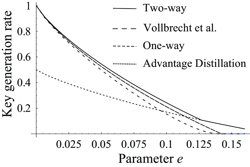
Figure 4.1: Comparison of the asymptotic key generation rates of the six-state protocols. “Two-way” is the asymptotic key generation rate of the proposed postprocessing. “Vollbrecht et al.” is the asymptotic key generation rate of the two-way postprocessing of [MFD⁺06, WMU06]. “Advantage Distillation” is the asymptotic key generation rate of the postprocessing with the advantage distillation [GL03]. “One-way” is the asymptotic key generation rate of the one-way postprocessing [RGK05]. It should be noted that the asymptotic key generation rates of the six-state protocols with the advantage distillation in [Ren05, GL03, Cha02, BA07] are slightly higher than that of the proposed protocol for much higher error rate.

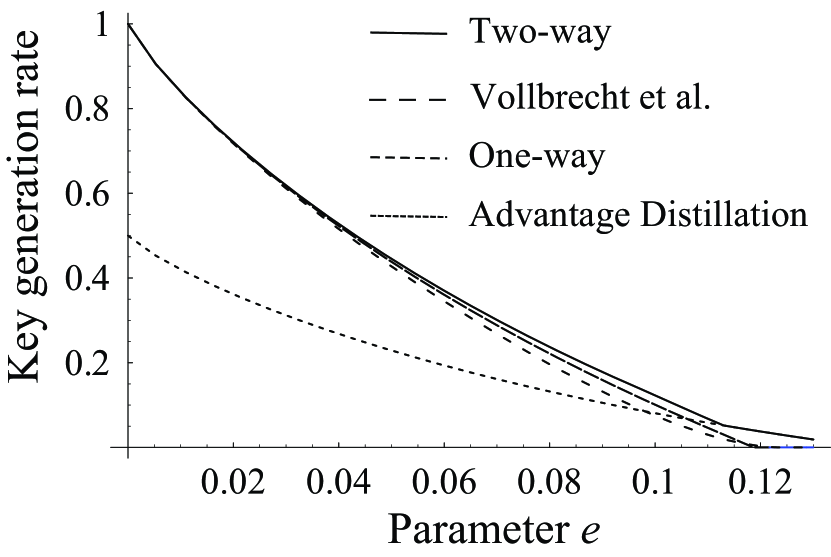
Figure 4.2: Comparison of the asymptotic key generation rates of the BB84 protocols. “Two-way” is the asymptotic key generation rate of the proposed postprocessing. “Vollbrecht et al.” is the asymptotic key generation rate of the two-way postprocessing of [MFD⁺06, WMU06]. “Advantage Distillation” is the asymptotic key generation rate of the postprocessing with the advantage distillation [GL03]. “One-way” is the asymptotic key generation rate of the one-way postprocessing [RGK05].

Proof of Theorem 4.5.3

Let

$$|\psi_{ABE}\rangle := \sum_{\mathsf{k},\mathsf{l}\in\mathbb{F}_{2}}\sqrt{P_{\mathsf{KL}}(\mathsf{k},\mathsf{l})}|\psi(\mathsf{k},\mathsf{l})\rangle|\mathsf{k},\mathsf{l}\rangle$$

$$= \sum_{x,\mathsf{k}\in\mathbb{F}_{2}}\sqrt{P_{\mathsf{K}}(\mathsf{k})}|x,x+\mathsf{k}\rangle|\phi(x,\mathsf{k})\rangle$$

be a purification of $\rho=\sum_{\mathsf{k},\mathsf{l}\in\mathbb{F}_{2}}|\psi(\mathsf{k},\mathsf{l})\rangle\langle\psi(\mathsf{k},\mathsf{l})|$, where we set

$$|\phi(x,\mathsf{k})\rangle:=\frac{1}{\sqrt{P_{\mathsf{K}}(\mathsf{k})}}\sum_{\mathsf{l}\in\mathbb{F}_{2}}(-1)^{x\mathsf{l}}\sqrt{P_{\mathsf{KL}}(\mathsf{k},\mathsf{l})}|\mathsf{k},\mathsf{l}\rangle,$$

and where $P_{\mathsf{K}}(\mathsf{k})=\sum_{\mathsf{l}\in\mathbb{F}_{2}}P_{\mathsf{KL}}(\mathsf{k},\mathsf{l})$ is a marginal distribution. Then, let

$$\rho_{X_{1}X_{2}Y_{1}Y_{2}E_{1}E_{2}}$$

$$= \sum_{\vec{x},\vec{\mathsf{k}}\in\mathbb{F}_{2}^{2}}\frac{1}{4}P_{\mathsf{K}}^{2}(\vec{\mathsf{k}})|\vec{x},\vec{x}+\vec{\mathsf{k}}\rangle\langle\vec{x},\vec{x}+\vec{\mathsf{k}}|\otimes\rho_{E_{1}E_{2}}^{\vec{x},\vec{\mathsf{k}}},$$

where

$$\rho_{E_{1}E_{2}}^{\vec{x},\vec{\mathsf{k}}}:=|\phi(x_{1},\mathsf{k}_{1})\rangle\langle\phi(x_{1},\mathsf{k}_{1})|\otimes|\phi(x_{2},\mathsf{k}_{2})\rangle\langle\phi(x_{2},\mathsf{k}_{2})|$$

for $\vec{x}=(x_{1},x_{2})$ and $\vec{\mathsf{k}}=(\mathsf{k}_{1},\mathsf{k}_{2})$.

Note that $H(U_{1}|Y_{1}Y_{2})=H(W_{1})$ for the Pauli channel. Let $W_{2}$ be a random variable defined by $W_{2}:=\xi_{2}(W_{1},Y_{2})+U_{2}$. Then, for the Pauli channel, we have $H(U_{2}|W_{1}Y_{1}Y_{2})=P_{W_{1}}(0)H(P_{W_{2}|W_{1}=0})$.

Noting that

$$P_{X_{1}X_{2}Y_{1}Y_{2}}(\vec{x},\vec{x}+\vec{\mathsf{k}})=\frac{1}{4}P_{\mathsf{K}}^{2}(\vec{\mathsf{k}}),$$

we have

$$P_{U_{1}}(u_{1}) = \frac{1}{2}$$

$$P_{W_{1}}(w_{1}) = \sum_{\vec{\mathsf{k}}\in\mathbb{F}_{2}^{2}\atop\mathsf{k}_{1}+\mathsf{k}_{2}=w_{1}}P_{\mathsf{K}}^{2}(\vec{\mathsf{k}})$$

$$P_{U_{2}|W_{1}=0}(u_{2}) = \frac{1}{2}$$

$$P_{U_{2}|W_{1}=1}(u_{2}) = 1$$

$$P_{W_{2}|W_{1}=0}(w_{2}) = \frac{P_{\mathsf{K}}^{2}(w_{2},w_{2})}{P_{W_{1}}(w_{1})}$$

$$P_{W_{2}|W_{1}=1}(0) = 1.$$

Using these formulas, we can write

$$\rho_{U_{1}U_{2}W_{1}E_{1}E_{2}}=\sum_{\vec{u}\in\mathbb{F}_{2}^{2}}\sum_{w_{1}\in\mathbb{F}_{2}}P_{U_{1}}(u_{1})P_{W_{1}}(w_{1})$$

$$~{}~{}~{}~{}~{}~{}~{}~{}~{}P_{U_{2}|W_{1}=w_{1}}(u_{2})|\vec{u},w_{1}\rangle\langle\vec{u},w_{1}|\otimes\bar{\rho}_{E_{1}E_{2}}^{\vec{u},w_{1}}$$

for $\vec{u}=(u_{1},u_{2})$, where

$$\bar{\rho}_{E_{1}E_{2}}^{\vec{u},w_{1}}:=\sum_{w_{2}\in\mathbb{F}_{2}}P_{W_{2}|W_{1}=0}(w_{2})\rho_{E_{1}E_{2}}^{\vec{u}G,(w_{1},w_{2})G}$$

for $w_{1}=0$ and a matrix $G=\left(\begin{array}[]{cc}1&1\\ 1&0\end{array}\right)$, and

$$\bar{\rho}_{E_{1}E_{2}}^{\vec{u},w_{1}}:=\sum_{a,b\in\mathbb{F}_{2}}\frac{1}{4}\rho_{E_{1}E_{2}}^{(u_{1},a)G,(w_{1},b)G}$$

for $w_{1}=1$.

Since supports of rank $1$ matrices $\{\rho_{E_{1}E_{2}}^{\vec{x},\vec{\mathsf{k}}}\}_{\vec{\mathsf{k}}\in\mathbb{F}_{2}^{2}}$ are orthogonal to each other, $\rho_{E_{1}E_{2}}^{\vec{u},w_{1}}$ for $w_{1}=0$ is already eigen value decomposed. Applying Lemma 4.5.4 for $\mathsf{J}=\{00,10\}$ and $C=C^{\bot}=\{00,11\}$, we can eigen value decompose $\rho_{E_{1}E_{2}}^{\vec{u},w_{1}}$ for $w_{1}=1$ as

$$\rho_{E_{1}E_{2}}^{\vec{u},w_{1}}=\sum_{b\in\mathbb{F}_{2}}\frac{1}{2}\sum_{\vec{\mathsf{j}}\in\mathsf{J}}P_{\mathsf{J}|\vec{\mathsf{K}}=\vec{\mathsf{k}}}(\vec{\mathsf{j}})|\vartheta((u_{1},0),\mathsf{k},\vec{\mathsf{j}})\rangle\langle\vartheta((u_{1},0),\mathsf{k},\vec{\mathsf{j}})|,$$

where we follow the notations in Lemma 4.5.4 for $m=2$.

Thus, we have

$$H(\rho_{U_{1}U_{2}W_{1}E_{1}E_{2}})$$ (4.32)

$$= H(P_{U_{1}})+H(P_{W_{1}})+\sum_{w_{1}\in\mathbb{F}_{2}}P_{W_{1}}(w_{1})\{H(P_{U_{2}|W_{1}=w_{1}})$$

$$+\sum_{\vec{u}\in\mathbb{F}_{2}^{2}}P_{U_{1}}(u_{1})P_{U_{2}|W_{1}=w_{1}}(u_{2})H(\rho_{E_{1}E_{2}}^{\vec{u},w_{1}})\}$$

$$= 1+H(P_{\bar{\mathsf{K}}})+P_{\bar{\mathsf{K}}}(0)\{1+H(P_{\vec{\mathsf{K}}|\bar{\mathsf{K}}=0})\}$$

$$~{}~{}+P_{\bar{\mathsf{K}}}(1)H(P_{\vec{\mathsf{K}}\mathsf{J}|\bar{\mathsf{K}}=1}).$$

Taking the partial trace of $\rho_{U_{1}U_{2}W_{1}E_{1}E_{2}}$ over systems $U_{1},U_{2}$, we have

$$\rho_{W_{1}E_{1}E_{2}} = \sum_{w_{1}\in\mathbb{F}_{2}}P_{W_{1}}(w_{1})|w_{1}\rangle\langle w_{1}|$$

$$\otimes\left(\sum_{\vec{u}\in\mathbb{F}_{2}^{2}}P_{U_{1}}P_{U_{2}|W_{1}=w_{1}}(u_{2})\bar{\rho}_{E_{1}E_{2}}^{\vec{u},w_{1}}\right).$$

Thus, we have

$$H(\rho_{W_{1}E_{1}E_{2}}) = H(P_{W_{1}})+\sum_{w_{1}\in\mathbb{F}_{2}}P_{W_{1}}(w_{1})$$ (4.33)

$$H\left(\sum_{\vec{u}\in\mathbb{F}_{2}^{2}}P_{U_{1}}P_{U_{2}|W_{1}=w_{1}}(u_{2})\bar{\rho}_{E_{1}E_{2}}^{\vec{u},w_{1}}\right)$$

$$= H(P_{\bar{\mathsf{K}}})+\sum_{\bar{\mathsf{k}}\in\mathbb{F}_{2}}P_{\bar{\mathsf{K}}}(0)H(P_{\vec{\mathsf{K}}\vec{\mathsf{L}}|\bar{\mathsf{K}}=\bar{\mathsf{k}}}).$$

Combining Eqs. (4.32) and (4.33), we have

$$H_{\rho}(U_{1}U_{2}|W_{1}E_{1}E_{2})-H(U_{1}|Y_{1}Y_{2})-H(U_{2}|U_{1}W_{1}Y_{1}Y_{2})$$

$$= H_{\rho}(U_{1}U_{2}|W_{1}E_{1}E_{2})-H(P_{W_{1}})-P_{W_{1}}(0)H(P_{W_{2}|W_{1}=0})$$

$$= 2-H(P_{\vec{\mathsf{K}}\vec{\mathsf{L}}})+P_{\bar{\mathsf{K}}}(1)\{H(P_{\vec{\mathsf{K}}\mathsf{J}|\bar{\mathsf{K}}=1})-1\}$$

$$= 2-2H(P_{\mathsf{K}\mathsf{L}})+P_{\bar{\mathsf{K}}}(1)h\left(\frac{p_{00}p_{10}+p_{01}p_{11}}{(p_{00}+p_{01})(p_{10}+p_{11})}\right).$$

On the other hand, by taking partial trace of $\rho_{U_{1}U_{2}W_{1}E_{1}E_{2}}$ over the system $U_{1}$, we have

$$\rho_{U_{1}W_{1}E_{1}E_{2}} = \sum_{u_{1},w_{1}\in\mathbb{F}_{2}}\frac{1}{2}P_{W_{1}}(w_{1})|u_{1},w_{1}\rangle\langle u_{1},w_{1}|$$

$$\otimes\left(\sum_{u_{2}\in\mathbb{F}_{2}}P_{U_{2}|W_{1}=w_{1}}(u_{2})\rho_{E_{1}E_{2}}^{(u_{1},u_{2}),w_{1}}\right).$$

Thus, we have

$$H(\rho_{U_{1}W_{1}E_{1}E_{2}}) = 1+H(P_{W_{1}})+\sum_{u_{1},w_{1}\in\mathbb{F}_{2}}\frac{1}{2}P_{W_{1}}(w_{1})$$

$$~{}~{}H\left(\sum_{u_{2}\in\mathbb{F}_{2}}P_{U_{2}|W_{1}=w_{1}}(u_{2})\rho_{E_{1}E_{2}}^{(u_{1},u_{2}),w_{1}}\right)$$

$$= 1+H(P_{\bar{\mathsf{K}}})+\sum_{\bar{\mathsf{k}}\in\mathbb{F}_{2}}P_{\bar{\mathsf{K}}}(\bar{\mathsf{k}})H(P_{\vec{\mathsf{K}}\mathsf{J}|\bar{\mathsf{K}}=1}).$$

Combining Eqs. (4.32) and (LABEL:entropy-uwe2), we have

$$H_{\rho}(U_{2}|W_{1}U_{1}E_{1}E_{2})-H(U_{2}|W_{1}U_{1}E_{1}E_{2})$$

$$= H_{\rho}(U_{2}|W_{1}U_{1}E_{1}E_{2})-P_{W_{1}}(0)H(P_{W_{2}|W_{1}=0})$$

$$= P_{\bar{\mathsf{K}}}(0)(1-H(P_{\mathsf{K}\mathsf{L}}^{\prime})).$$

∎

Lemma 4.5.4

Let $C$ be a linear subspace of $\mathbb{F}_{2}^{m}$. Let

$$|\varphi^{m}(\vec{x},\vec{\mathsf{k}})\rangle:=\frac{1}{\sqrt{P_{\mathsf{K}}^{m}(\vec{\mathsf{k}})}}\sum_{\vec{\mathsf{l}}\in\mathbb{F}_{2}^{m}}(-1)^{\vec{x}\cdot\vec{\mathsf{l}}}\sqrt{P_{\mathsf{KL}}^{m}(\vec{\mathsf{k}},\vec{\mathsf{l}})}|\vec{\mathsf{k}},\vec{\mathsf{l}}\rangle,$$

and $\rho_{E^{m}}^{\vec{x},\vec{\mathsf{k}}}:=|\varphi^{m}(\vec{x},\vec{\mathsf{k}})\rangle\langle\varphi^{m}(\vec{x},\vec{\mathsf{k}})|$. Let $\mathsf{J}$ be a set of coset representatives of the cosets $\mathbb{F}_{2}^{m}/C$, and

$$P_{\mathsf{J}|\mathsf{K}^{m}=\vec{\mathsf{k}}}(\vec{\mathsf{j}}):=\frac{\sum_{\vec{\mathsf{c}}\in C^{\bot}}P_{\mathsf{KL}}^{m}(\vec{\mathsf{k}},\vec{\mathsf{j}}+\vec{\mathsf{c}})}{P_{\mathsf{K}}^{m}(\vec{\mathsf{k}})}$$

be conditional probability distributions on $\mathsf{J}$. Then, for any $\vec{a}\in\mathbb{F}_{2}^{m}$, we have

$$\sum_{\vec{x}\in C}\frac{1}{|C|}\rho_{E^{m}}^{\vec{x}+\vec{a},\vec{\mathsf{k}}}=\sum_{\vec{\mathsf{j}}\in\mathsf{J}}P_{\mathsf{J}|\mathsf{K}^{m}=\vec{\mathsf{k}}}(\vec{\mathsf{j}})|\vartheta(\vec{a},\vec{\mathsf{k}},\vec{\mathsf{j}})\rangle\langle\vartheta(\vec{a},\vec{\mathsf{k}},\vec{\mathsf{j}})|,$$ (4.35)

where

$$|\vartheta(\vec{a},\vec{\mathsf{k}},\vec{\mathsf{j}})\rangle := \frac{1}{\sqrt{\sum_{\vec{\mathsf{e}}\in C^{\bot}}P_{\mathsf{KL}}^{m}(\vec{\mathsf{k}},\vec{\mathsf{j}}+\vec{\mathsf{e}})}}$$

$$\sum_{\vec{\mathsf{c}}\in C^{\bot}}(-1)^{\vec{a}\cdot\vec{\mathsf{c}}}\sqrt{P_{\mathsf{KL}}^{m}(\vec{\mathsf{k}},\vec{\mathsf{j}}+\vec{\mathsf{c}})}|\vec{\mathsf{k}},\vec{\mathsf{j}}+\vec{\mathsf{c}}\rangle.$$

Remark 4.5.5

If $\vec{\mathsf{j}}\neq\vec{\mathsf{i}}$, obviously we have $\langle\vartheta(\vec{a},\vec{\mathsf{k}},\vec{\mathsf{j}})|\vartheta(\vec{a},\vec{\mathsf{k}},\vec{\mathsf{i}})\rangle=0$. Thus, the right hand side of Eq. (4.35) is an eigen value decomposition. Moreover, if $\vec{a}+\vec{b}\in C$, then we have $|\vartheta(\vec{a},\vec{\mathsf{k}},\vec{\mathsf{j}})\rangle=|\vartheta(\vec{b},\vec{\mathsf{k}},\vec{\mathsf{j}})\rangle$.

Proof.

For any $\vec{x}\in C$ and $\vec{a}\in\mathbb{F}_{2}^{m}$, we can rewrite

$$|\varphi(\vec{x}+\vec{a},\vec{\mathsf{k}})\rangle = \frac{1}{\sqrt{P_{\mathsf{K}}^{m}(\vec{\mathsf{k}})}}\sum_{\vec{\mathsf{j}}\in\mathsf{J}}\sum_{\vec{\mathsf{c}}\in C^{\bot}}(-1)^{(\vec{x}+\vec{a})\cdot(\vec{\mathsf{j}}+\vec{\mathsf{c}})}$$

$$~{}~{}~{}\sqrt{P_{\mathsf{KL}}^{m}(\vec{\mathsf{k}},\vec{\mathsf{j}}+\vec{\mathsf{c}})}|\vec{\mathsf{k}},\vec{\mathsf{j}}+\vec{\mathsf{c}}\rangle$$

$$= \sum_{\vec{\mathsf{j}}\in\mathsf{J}}(-1)^{(\vec{x}+\vec{a})\cdot\vec{\mathsf{j}}}\sqrt{P_{\mathsf{J}|\mathsf{K}^{m}=\vec{\mathsf{k}}}(\vec{\mathsf{j}})}|\vartheta(\vec{a},\vec{\mathsf{k}},\vec{\mathsf{j}})\rangle.$$

Then, we have

$$\sum_{\vec{x}\in C}\frac{1}{|C|}\rho_{E^{m}}^{\vec{x}+\vec{a},\vec{\mathsf{k}}}$$

$$= \sum_{\vec{x}\in C}\frac{1}{|C|}\sum_{\vec{\mathsf{i}},\vec{\mathsf{j}}\in\mathsf{J}}(-1)^{(\vec{x}+\vec{a})\cdot(\vec{\mathsf{i}}+\vec{\mathsf{j}})}\sqrt{P_{\mathsf{J}|\mathsf{K}^{m}=\vec{\mathsf{k}}}(\vec{\mathsf{i}})P_{\mathsf{J}|\mathsf{K}^{m}=\vec{\mathsf{k}}}(\vec{\mathsf{j}})}$$

$$~{}~{}~{}|\vartheta(\vec{a},\vec{\mathsf{k}},\vec{\mathsf{i}})\rangle\langle\vartheta(\vec{a},\vec{\mathsf{k}},\vec{\mathsf{j}})|$$

$$= \sum_{\vec{\mathsf{i}},\vec{\mathsf{j}}\in\mathsf{J}}(-1)^{\vec{a}\cdot(\vec{\mathsf{i}}+\vec{\mathsf{j}})}\sum_{\vec{x}\in C}\frac{1}{|C|}(-1)^{\vec{x}\cdot(\vec{\mathsf{i}}+\vec{\mathsf{j}})}\sqrt{P_{\mathsf{J}|\mathsf{K}^{m}=\vec{\mathsf{k}}}(\vec{\mathsf{i}})P_{\mathsf{J}|\mathsf{K}^{m}=\vec{\mathsf{k}}}(\vec{\mathsf{j}})}$$

$$~{}~{}~{}|\vartheta(\vec{a},\vec{\mathsf{k}},\vec{\mathsf{i}})\rangle\langle\vartheta(\vec{a},\vec{\mathsf{k}},\vec{\mathsf{j}})|$$

$$= \sum_{\vec{\mathsf{j}}\in\mathsf{J}}P_{\mathsf{J}|\mathsf{K}^{m}=\vec{\mathsf{k}}}(\vec{\mathsf{j}})|\vartheta(\vec{a},\vec{\mathsf{k}},\vec{\mathsf{j}})\rangle\langle\vartheta(\vec{a},\vec{\mathsf{k}},\vec{\mathsf{j}})|,$$

where $\cdot$ is the standard inner product on the vector space $\mathbb{F}_{2}^{m}$, and we used the following equality,

$$\sum_{\vec{x}\in C}(-1)^{\vec{x}\cdot(\vec{\mathsf{i}}+\vec{\mathsf{j}})}=0$$

for $\vec{\mathsf{i}}\neq\vec{\mathsf{j}}$. ∎

4.5.2 Unital Channel

In this section, we calculate the asymptotic key generation rates for the Unital channel. Although we succeeded to show a closed formula of the asymptotic key generation rate for the Pauli channel, which is a special class of the unital channel, in Section 4.5.1, we do not know any closed formula of the asymptotic key generation rate for the unital channel in general.

For the six-state protocol, it is straightforward to numerically calculate the asymptotic key generation rate. For the BB84 protocol, owing to Proposition 4.4.5, the asymptotic key generation rate can be calculated by taking the minimization over one free parameter $R_{\mathsf{yy}}$.

As an example of non Pauli but unital channel, we numerically calculated asymptotic key generation rates for the depalarizing channel whose axis is rotated by $\pi/4$, i.e., the channel whose Stokes parameterization is given by

$$\left(\left[\begin{array}[]{ccc}\cos(\pi/4)&-\sin(\pi/4)&0\\ \sin(\pi/4)&\cos(\pi/4)&0\\ 0&0&1\end{array}\right]\left[\begin{array}[]{ccc}1-2e&0&0\\ 0&1-2e&0\\ 0&0&1-2e\end{array}\right],\left[\begin{array}[]{c}0\\ 0\\ 0\end{array}\right]\right).$$ (4.45)

For this channel, since the Choi operator is symmetric with respect to Alice and Bob’s subsystem, we can also show that the asymptotic key generation rate is maximized when we employ the functions $\chi_{A},\chi_{B}$ given by Eqs. (4.13) and (4.14) in a similar manner as Lemma 4.5.2. Therefore, we employ the functions given by Eqs. (4.13) and (4.14) throughout this subsection. Furthermore, we can find that the asymptotic key generation rates for the direct and the reverse IR procedure coincide, because $H_{\rho}(U_{1}|W_{1}E_{1}E_{2})=H_{\rho}(V_{1}|W_{1}E_{1}E_{2})$ and $H_{\rho}(U_{1}|Y_{1}Y_{2})=H_{\rho}(V_{1}|X_{1}X_{2})$. Therefore, we only consider the asymptotic key generation rate for the direct IR procedure throughout this subsection.

For the BB84 protocol and the six-state protocol, the asymptotic key generation rate of the postprocessing with the two-way IR procedure and that of the postprocessing with the one-way IR procedure are compared in Fig. 4.3 and Fig. 4.4 respectively. We find that the asymptotic key generation rates of the postprocessing with our proposed two-way IR procedure is higher than those of the one-way postprocessing, which suggest that our proposed IR procedure is effective not only for the Pauli channel, but also for non-Pauli channels. It should be noted that the asymptotic key generation rates of the postprocessing with the direct one-way IR procedure and the reverse one-way IR procedure coincide for this example.

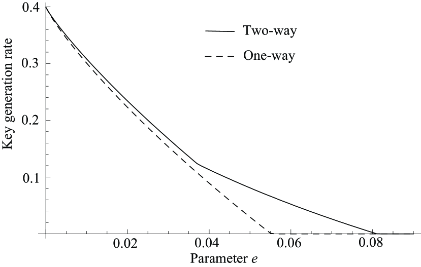
Figure 4.3: Comparison of the asymptotic key generation rates of the BB84 protocol. “Two-way” is the asymptotic key generation rate of the postprocessing with two-way IR procedure (Eq. (4.8)). “One-way” is the asymptotic key generation rate of the postprocessing with one-way IR procedure (Eq. (3.15)).

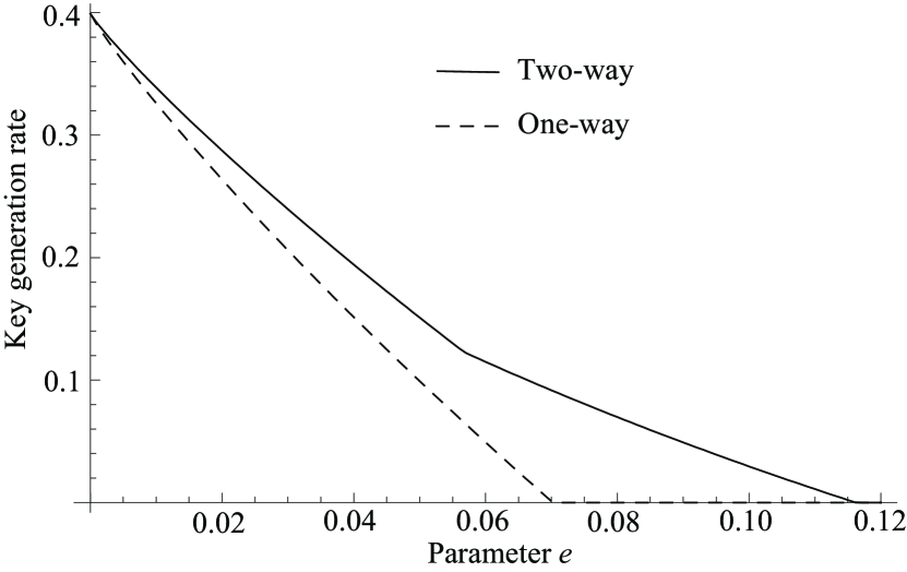
Figure 4.4: Comparison of the asymptotic key generation rates of the six-state protocol. “Two-way” is the asymptotic key generation rate of the postprocessing with two-way IR procedure (Eq. (4.6)). “One-way” is the asymptotic key generation rate of the postprocessing with one-way IR procedure (Eq. (3.12)).

4.5.3 Amplitude Damping Channel

In this section, we calculate the asymptotic key generation rates (for the direct two-way IR procedure and the reverse two-way IR procedure) for the amplitude damping channel. Although we succeeded to derive a closed formulae of the asymptotic key generation rates of the one-way postprocessing in Section 3.6.1, we do not know any closed formula of the asymptotic key generation rates of the postprocessing with the two-way IR procedure for the amplitude damping channel. Furthermore, it is not clear whether the asymptotic key generation rate is maximized when we employ the functions given by Eqs. (4.13) and (4.14). Therefore, we (numerically) optimize the choice of the functions $\chi_{A},\chi_{B}$ so that the asymptotic key generation rate is maximized.

Since the set ${\cal P}_{c}(\omega)$ consists of only $\rho$ itself for both the BB84 protocol (refer Section 3.6.1), we can easily conduct the numerical calculation of the asymptotic key generation rates for the six-state protocol and the BB84 protocol. The asymptotic key generation rates of the postprocessing with the direct two-way IR procedure, the reverse two-way IR procedure, the direct one-way IR procedure, and the reverse one-way IR procedure are compared in Fig. 4.5. It should be noted that the asymptotic key generation rates for the BB84 protocol and the six-state protocol coincide in this example. We numerically found that the functions given by $\chi_{A}(a_{1},a_{2}):=1$ and

$$\chi_{B}(a_{1},a_{2})=\left\{\begin{array}[]{ll}0&\mbox{if }a_{1}=a_{2}\\ 1&\mbox{else}\end{array}\right.$$

maximizes the asymptotic key generation rates for both the direct two-way IR procedure and the reverse IR procedure.

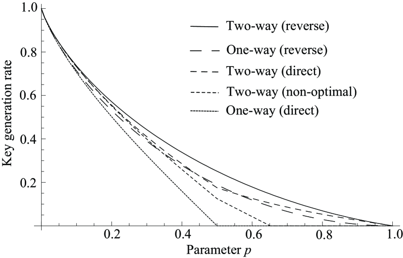
Figure 4.5: Comparison of the asymptotic key generation rates. “Two-way (reverse)” is the asymptotic key generation rate of the postprocessing with reverse two-way IR procedure (Eq. (4.7)). “One-way (reverse)” is the asymptotic key generation rate of the postprocessing with reverse one-way IR procedure (Eq. (3.13)). “Two-way (direct)” is the asymptotic key generation rate of the postprocessing with direct two-way IR procedure (Eq. (4.6)). “Two-way (non-optimal)” is the asymptotic key generation rate of the postprocessing with direct two-way IR procedure when we employ the functions $\chi_{A},\chi_{B}$ given by Eqs. (4.13) and (4.14). “One-way (direct)” is the asymptotic key generation rate of the postprocessing with one-way IR procedure (Eq. (3.12)).

4.6 Relation to Entanglement Distillation Protocol

As is mentioned in Chapter 1, the security of the QKD protocols have been studied by using the quantum error correcting code and the entanglement distillation protocol (EDP) since Shor and Preskill found the relation between them [SP00]. The crucial point in Shor and Preskill’s proof is to find an EDP that corresponds to a postprocessing of the QKD protocols. Indeed, the security of the QKD protocols with the two-way classical communication [GL03] was proved by finding the corresponding EDPs.

We will explain the EDP proposed by Vollbrecht and Vestraete [VV05] in this section. Then, we present the postprocesing of the QKD protocols that corresponds to Vollbrecht and Vestraete’s EDP. Furthermore, we compare the posptocessing (corresponding to Vollbrecht and Vestraete’s EDP) and the postprocessing shown in Section 4.4, and clarify the relation between them, where we employ the functions given by Eqs. (4.13) and (4.14). The comparison result suggests that there exists no EDP that corresponds to the postprocessing shown in Section 4.4.

Suppose that Alice and Bob share $2n$ pairs bipartite qubits systems, and the state of each bipartite system is a Bell diagonal state

$$\rho=\sum_{\mathsf{k},\mathsf{l}\in\mathbb{F}_{2}}P_{\mathsf{KL}}(\mathsf{k},\mathsf{l})|\psi(\mathsf{k},\mathsf{l})\rangle\langle\psi(\mathsf{k},\mathsf{l})|.$$ (4.47)

The EDP is a protocol to distill the mixed entangled state $\rho^{\otimes 2n}$ into the maximally entangled state $|\psi\rangle^{\otimes\ell}$ by using the local operation and the classical communication [BDSW96].

Vollbrecht and Vestraete proposed the following EDP [VV05], where it is slightly modified (essentially the same) from the original version because we want to clarify the relation among this EDP, the corresponding postprocessing, and the postprocessing shown in Section 4.4.

1. Alice and Bob divide $2n$ pairs of the bipartite systems into $n$ blocks of length $2$, and locally carry out the controlled-NOT (CNOT) operation on each block, where the $2i$th pair is the source and the $(2i-1)$th pair is the target.

2. Then, Alice and Bob undertake the breeding protocol [BBP⁺96] to guess bit-flip errors in the $(2i-1)$th pair for all $i$. The guessed bit-flip errors can be described by a sequence $\hat{\mathbf{w}}_{1}$ (Note that two-way classical communication is used in this step).

3. According to $\hat{\mathbf{w}}_{1}$, Alice and Bob classify indices of blocks into two sets $\mathsf{T}_{0}:=\{i:~{}\hat{w}_{i}=0\}$ and $\mathsf{T}_{1}:=\{i:~{}\hat{w}_{i}=1\}$.

4. For a collection of $2i$th pairs such that $i\in\mathsf{T}_{0}$, Alice and Bob conduct the breeding protocol to correct bit-flip errors.

5. For a collection of $2i$th pairs such that $i\in\mathsf{T}_{1}$, Alice and Bob perform measurements in the $\mathsf{z}$-basis, and obtain measurement results $\mathbf{x}_{2,\mathsf{T}_{1}}$ and $\mathbf{y}_{2,\mathsf{T}_{1}}$ respectively.

6. Alice sends $\mathbf{x}_{2,\mathsf{T}_{1}}$ to Bob.

7. Alice and Bob correct the phase errors for the remaining pairs by using information $\mathsf{T}_{0}$, $\mathsf{T}_{1}$, and the bit-flip error $\mathbf{x}_{2,\mathsf{T}_{1}}+\mathbf{y}_{2,\mathsf{T}_{1}}$.

The yield of this EDP is given by

$$1-H(P_{\mathsf{KL}})+\frac{P_{\bar{\mathsf{K}}}(1)}{4}\left\{h\left(\frac{p_{01}}{p_{00}+p_{01}}\right)+h\left(\frac{p_{11}}{p_{10}+p_{11}}\right)\right\}.$$ (4.48)

We can find by the concavity of the binary entropy function that the first argument in the maximum of the r.h.s. of Eq. (4.31) is larger than the value in Eq. (4.48).

If we convert this EDP into a postprocessing of the QKD protocols, the difference between that postprocessing and ours is as follows. In the postprocessing converted from the EDP [VV05], after Step (iv), Alice reveals the sequence, $\mathbf{x}_{2,\hat{\mathsf{T}}_{1}}$, which consists of the second bit, $x_{i2}$, of the $i$th block such that the parity of discrepancies $\hat{w}_{i1}$ is $1$. However, Alice discards $\mathbf{x}_{2,\hat{\mathsf{T}}_{1}}$ in the proposed IR protocol of Section 4.3. Since sequence $\mathbf{x}_{2,\hat{\mathsf{T}}_{1}}$ has some correlation to sequence $\mathbf{u}_{1}$ from the view point of Eve, Alice should not reveal $\mathbf{x}_{2,\hat{\mathsf{T}}_{1}}$ to achieve a higher key generation rate.

In the EDP context, on the other hand, since the bit flip error, $\mathbf{x}_{2,\hat{\mathsf{T}}_{1}}+\mathbf{y}_{2,\hat{\mathsf{T}}_{1}}$, has some correlation to the phase flip errors in the $(2i-1)$-th pair with $i\in\hat{\mathsf{T}}_{1}$, Alice should send the measurement results, $\mathbf{x}_{2,\hat{\mathsf{T}}_{1}}$, to Bob. If Alice discards measurement results $\mathbf{x}_{2,\hat{\mathsf{T}}_{1}}$ without telling Bob what the result is, then the yield of the resulting EDP is worse than Eq. (4.48). Consequently, there seems to be no correspondence between the EDP and our proposed classical processing.

4.7 Summary

The results in this chapter is summarized as follows: In Section 4.2, we reviewed the advantage distillation. In Section 4.3, we proposed the two-way IR procedure. In Section 4.4, we derived a sufficient condition on the key generation rate such that a secure key agreement is possible with our proposed postprocessing (Theorem 4.4.1). We also derived the asymptotick key generation rate formulae.

In Section 4.5, we investigated the asymptotic key generation rate of our proposed postprocessing. Especially in Section 4.5.1, we derived a closed form of the asymptotic key generation rate for the Pauli channel (Theorem 4.5.3), which clarifies that the asymptotic key generation rate of our proposed postprocessing is at least as high as the asymptotic key generation rate of the standard postprocessing. We also numerically clarified that the asymptotic key generation rate of our proposed postprocessing is higher than the asymptotic key generation rate of any other postprocessing for the Pauli channel (Section 4.5.1), the unital channel (Section 4.5.2), and the amplitude damping channel (Section 4.5.3) respectively.

Finally in Section 4.6, we clarified the relation between our proposed postprocessing and the EDP proposed by Vollbrecht and Vestraete [VV05].

Chapter 5 Conclusion

In this thesis, we investigated the channel estimation phase and the postprocessing phase of the QKD protocols. The contribution of this thesis is summarized as follows.

For the channel estimation phase, we proposed a new channel estimation procedure in which we use the mismatched measurement outcomes in addition to the samples from the matched measurement outcomes. We clarified that the key generation rate decided according to our proposed channel estimation procedure is at least as high as the key generation rate decided according to the conventional channel estimation procedure. We also clarified that the former is strictly higher than the latter for the amplitude damping channel and the unital channel.

For the postprocessing phase, we proposed a new kind of postprocessing procedure with two-way public communication. For the Pauli channel, we clarified that the key generation rate of the QKD protocols with our proposed postprocessing is higher than the key generation rate of the QKD protocols with the standard one-way postprocessing. For the Pauli channel, the amplitude damping channel, and the unital channel, we numerically clarified that the QKD protocols with our proposed postprocessing is higher than the key generation rate of the QKD protocols with any other postprocessing.

There are some problems that should be investigated in a future.

• To show the necessary and sufficient condition on the channel for that the (asymptotic) key generation rate decided according our proposed channel estimation procedure is strictly higher than that decided according to the conventional channel estimation procedure for the six-state protocol.

• To analytically show that the (asymptotic) key generation rate of our proposed two-way postprocessing is at least as high as that of the standard one-way postprocessing, or to find a counter example.

Appendix A Notations

Notations first appeared in Chapter 2

${\cal P}({\cal X})$	the set of all probability distributions on the set ${\cal X}$
$P_{X},P_{XY}$	probability distributions
$P_{\mathbf{x}}$	the type of the sequence $\mathbf{x}$
${\cal P}({\cal H})$	the set of all density operators on the quantum system ${\cal H}$
${\cal P}^{\prime}({\cal H})$	the set of all non-negative operators on ${\cal H}$
$\rho,\rho_{AB}$	density operators
$\|\cdot\|$	the trace distance (variational distance)
$F(\cdot,\cdot)$	the fidelity
$H(X)$	the entropy of the random variable $X$
$H(P_{X})$	the entropy of the random variable with the distribution $P_{X}$
$h(\cdot)$	the binary entropy function
$H(X|Y)$	the (Shannon) conditional entropy of $X$ given $Y$
$I(X;Y)$	the mutual information between $X$ and $Y$
$H(\rho)$	the von Neumann entropy of the system whose state is $\rho$
$H_{\rho}(A|B)$	the conditional von Neumann entropy of the system $A$ conditioned by the system $B$
$I_{\rho}(A;B)$	the quantum mutual information between the systems $A$ and $B$
$\sigma_{\mathsf{x}},\sigma_{\mathsf{y}},\sigma_{\mathsf{z}}$	the Pauli operators
$|\psi\rangle$	the maximally entangled state defined in Eq. (2.9)
${\cal P}_{c}$	the set of all Choi operators
$(R,t)$	the Stokes parameterization of the channel
$H_{\min}(\rho_{AB}|\sigma_{B})$	the min-entropy of $\rho_{AB}$ relative to $\sigma_{B}$
$H_{\max}(\rho_{AB}|\sigma_{B})$	the max-entropy of $\rho_{AB}$ relative to $\sigma_{B}$
$H_{\min}^{\varepsilon}(\rho_{AB}|B)$	the $\varepsilon$-smooth min-entropy of $\rho_{AB}$ given the system $B$
$H_{\max}^{\varepsilon}(\rho_{AB}|B)$	the $\varepsilon$-smooth max-entropy of $\rho_{AB}$ given the system $B$
${\cal B}^{\varepsilon}(\rho)$	the set of all operators $\bar{\rho}\in{\cal P}^{\prime}({\cal H})$ such that $\|\bar{\rho}-\rho\|\leq\mathrm{Tr}[\rho]\varepsilon$
$d(\rho_{AB}|B)$	the distance from the uniform (see Definition 2.2.11)

Notations first appeared in Chapter 3

$|0_{\mathsf{a}}\rangle,|1_{\mathsf{a}}\rangle$	the eigenstates of the Pauli operator $\sigma_{\mathsf{a}}$
$\rho_{\mathbf{X}\mathbf{Y}\mathbf{E}}$	the $\{ccq\}$-state describing Alice and Bob’s bit sequences $(\mathbf{X},\mathbf{Y})$ and the state in Eve’s system
$M$	the parity check matrix
$t$	the syndrome
$P_{XY}$	the probability distribution of Alice and Bob’s bits
$P_{W}$	the probability distribution of the discrepancy between Alice and Bos’s bits
$\omega$	the components $(R_{\mathsf{zz}},R_{\mathsf{zx}},R_{\mathsf{xz}},R_{\mathsf{xx}},t_{\mathsf{z}},t_{\mathsf{x}})$ of the Stokes parameterization
$\tau$	the components $(R_{\mathsf{zy}},R_{\mathsf{xy}},R_{\mathsf{yz}},R_{\mathsf{yx}},R_{\mathsf{yy}},t_{\mathsf{y}})$ of the Stokes parameterization
$\Omega$	the range of $\omega$
${\cal P}_{c}(\omega)$	the set of all Choi operator for a fixed $\omega$
$\gamma$	the components $(R_{\mathsf{zz}},R_{\mathsf{xx}},R_{\mathsf{yy}})$ of the Stokes parameterization
$\kappa$	the components $(R_{\mathsf{zx}}$,$R_{\mathsf{zy}}$,$R_{\mathsf{xz}}$,$R_{\mathsf{xy}}$,$R_{\mathsf{yz}}$,$R_{\mathsf{yx}}$,$t_{\mathsf{z}}$,$t_{\mathsf{x}}$,$t_{\mathsf{y}})$ of the Stokes parameterization
$\Gamma$	the range of $\gamma$
${\cal P}_{c}(\gamma)$	the set of all Choi operator for a fixed $\gamma$
$\upsilon$	the components $(R_{\mathsf{zz}},R_{\mathsf{xx}})$ of the Stokes parameterization
$\varsigma$	the components $(R_{\mathsf{zx}}$,$R_{\mathsf{zy}}$,$R_{\mathsf{xz}}$,$R_{\mathsf{xy}}$,$R_{\mathsf{yz}}$,$R_{\mathsf{yx}}$,$R_{\mathsf{yy}}$,$t_{\mathsf{z}}$,$t_{\mathsf{x}}$,$t_{\mathsf{y}})$ of the Stokes parameterization
$\Upsilon$	the range of $\upsilon$
${\cal P}_{c}(\upsilon)$	the set of all Choi operators for a fixed $\upsilon$

Notations first appeared in Chapter 4

$\xi$	the function $\xi:\mathbb{F}_{2}^{2}\to\mathbb{F}_{2}$ such that $\xi(a_{1},a_{2})=a_{1}+a_{2}$
$\zeta$	the function $\zeta:\mathbb{F}_{2}^{2}\to\mathbb{F}_{2}$ such that $\zeta(a,0)=a$ and $\zeta(a,1)=0$
$\chi_{A},\chi_{B}$	arbitrary functions from $\mathbb{F}_{2}^{2}$ to $\mathbb{F}_{2}$
$\zeta_{A}$	the function $\mathbb{F}_{2}^{3}\to\mathbb{F}_{2}$ such that $\zeta_{A}(a_{1},a_{2},a_{3})=a_{1}$ for $\chi_{A}(a_{2},a_{3})=0$ and $\zeta_{A}(a_{1},a_{2},a_{3})=0$ for else
$\zeta_{B}$	the function $\mathbb{F}_{2}^{3}\to\mathbb{F}_{2}$ such that $\zeta_{B}(a_{1},a_{2},a_{3})=a_{1}$ for $\chi_{B}(a_{2},a_{3})=0$ and $\zeta_{B}(a_{1},a_{2},a_{3})=0$ for else
$U_{1}$	the random variable defined as $U_{1}=\xi(X_{1},X_{2})$
$V_{1}$	the random variable defined as $V_{1}=\xi(Y_{1},Y_{2})$
$W_{1}$	the random variable defined as $W_{1}=U_{1}+V_{1}$
$U_{2}$	the random variable defined as $U_{2}=\zeta(X_{2},W_{1})$ or the random variable defined as $U_{2}=\zeta_{A}(X_{2},U_{1},V_{1})$
$V_{2}$	the random variable defined as $V_{2}=\zeta(Y_{2},W_{1}$ or the random variable defined as $V_{2}=\zeta_{B}(X_{2},U_{1},V_{1})$
$|\psi(\mathsf{k},\mathsf{l})\rangle$	Bell states
$P_{\mathsf{KL}}$	the distribution such that the Bell diagonal components of a Bell diagonal state

Appendix B Publications Related to This Thesis

Articles in Journals

• S. Watanabe, R. Matsumoto, T. Uyematsu, and Y. Kawano, ”Key rate of quantum key distribution with hashed two-way classical communication,” Phys. Rev. A, vol. 76, no. 3,pp. 032312-1–7, Sep. 2007.

• S. Watanabe, R. Matsumoto, and T. Uyematsu, ”Tomography increases key rate of quantum-key-distribution protocols,” Phys. Rev. A, vol. 78, no. 4, pp. 042316-1–11, Oct. 2008.

Peer-Reviewed Articles in International Conferences

• S. Watanabe, R. Matsumoto, and T. Uyematsu, ”Security of quantum key distribution protocol with two-way classical communication assisted by one-time pad encryption,” in Proc. Asian Conference on Qauntum Information Science 2006, Beijing, China, September 2006.

• S. Watanabe, R. Matsumoto, T. Uyematsu, and Y. Kawano, ”Key rate of quantum key distribution with hashed two-way classical communication,” in Proc. 2007 IEEE Int. Symp. Inform. Theory, Nice, France, June, 2007.

Non-Reviewd Articles in Conferences

• S. Watanabe, R. Matsumoto, T. Uyematsu, and Y. Kawano, ”Key rate of quantum key distribution with hashed two-way classical communication,” in Proc. QIT 16, Atsugi, Japan, May, 2006.

• S. Watanabe, R. Matsumoto, and T. Uyematsu, ”Tomography increases key rate of quantum-key-distribution protocols,” presented at recent result session in 2008 IEEE Int. Symp. Inform. Theory, Toronto, Canada, July, 2008.

• S. Watanabe, R. Matsumoto, and T. Uyematsu, ”Tomography increases key rate of quantum-key-distribution protocols,” in Proc. SITA 2008, Kinugawa, Japan, Oct., 2008.

• S. Watanabe, R. Matsumoto, and T. Uyematsu, ”Tomography increases key rate of quantum-key-distribution protocols,” presented at GSIS Workshop on Quantum Information Theory, Sendai, Japan, November 2008.

Bibliography

• [AC93] R. Ahlswede and I. Csiszár. Common randomness in information theory and cryptography–part 1: Secret sharing. IEEE Trans. Inform. Theory, 39(4):1121–1132, 1993.
• [BA07] J. Bae and A. Acín. Key distillation from quantum channels using two-way communication protocol. Phys. Rev. A, 75(1):012334, Jan. 2007. arXiv:quant-ph/0610048.
• [BB83] C. H. Bennett and G. Brassard. Quantum cryptography and its application to provably secure key expansion, public-key distribution, and coin-tossing. In Proceedings of IEEE International Symposium on Information Theory, page 91, St. Jouvite, Canada, Sep. 1983.
• [BB84a] C. H. Bennett and G. Brassard. Quantum cryptography: Public key distribution and coin tossing. In Proceedings of IEEE International Conference on Computers Systems and Signal Processing, pages 175–179, Bangalore, India, Dec. 1984.
• [BB84b] C. H. Bennett and G. Brassard. An update on quantum cryptography. In Advances in Cryptology CRYPTO 84, volume 196 of Lecture Notes in Computer Science, pages 475–480, Santa Barbara, California, Aug. 1984.
• [BB89] C. H. Bennett and G. Brassard. The dawn of a new era for quantum cryptography: The experiment prototype is working. Sigact News, 20(4):78–82, 1989.
• [BBB+92] C. H. Bennett, F. Bessette, G. Brassard, L. Salvail, and J. Smolin. Experimental quantum cryptography. Journal of Cryptology, 5(1):3–28, 1992.
• [BBB+00] E. Biham, M. Boyer, P. O. Boykin, T. Mor, and V. Roychowdhury. A proof of the security of quantum key distribution. Proc. 32-nd Annu. ACM Symp. Theory of Computing, pages 715–724, 2000. arXiv:quant-ph/9912053.
• [BBB+06] E. Biham, M. Boyer, P. O. Boykin, T. Mor, and V. Roychowdhury. A proof of the security of quantum key distribution. J. Cryptology, 19(4):381–439, October 2006. arXiv:quant-ph/0511175.
• [BBBW82] C. H. Bennett, G. Brassard, S. Breidart, and S. Wiesner. Quantum cryptography, or unforgeable subway tokens. In Advances in Cryptology CRYPTO 82, Lecture Notes in Computer Science, pages 175–179, Santa Barbara, California, 1982.
• [BBCM95] C. H. Bennett, G. Brassard, C. Crépeau, and U. Maurer. Generalized privacy amplification. IEEE Trans. on Inform. Theory, 41(6):1915–1923, Nov. 1995.
• [BBL05] J. C. Boileau, J. Batuwantudawe, and R. Laflamme. Higher-security thresholds for quantum key distribution by improved analysis of dark counts. Phys. Rev. A, 72(3):032321, September 2005. arXiv:quant-ph/0502140.
• [BBM92] C. H. Bennett, G. Brassard, and N. D. Mermin. Quantum cryptography without Bell’s theorem. Phys. Rev. Lett., 68:557–559, Feb. 1992.
• [BBP+96] C. H. Bennett, G. Brassard, S. Popescu, B. Schumacher, J. A. Smolin, and W. K. Wootters. Purification of noisy entanglement and faithful teleportation via noisy channels. Phys. Rev. Lett., 76(5):722–725, Jan. 1996. arXiv:quant-ph/9511027.
• [BBR85] C. H. Bennett, G. Brassard, and J. M. Robert. How to reduce your enemy’s information. In Advances in Cryptology CRYPTO 85, volume 218 of Lecture Notes in Computer Science, pages 468–476, Santa Barbara, California, Aug. 1985.
• [BBR88] C. H. Bennett, G. Brassard, and J. M. Robert. Privacy amplification by public discussion. SIAM Journal on Computing, 17(2):210–229, Apr. 1988.
• [BCE+03] D. Bruß, M. Christandl, A. Ekert, B. G. Englert, D. Kaszlikowski, and C. Macchiavello. Tomographic quantum cryptography: Equivalence of quantum and classical key distillation. Phys. Rev. Lett., 91(9):097901, August 2003. arXiv:quant-ph/0303184.
• [BDSW96] C. H. Bennett, D. P. DiVincenzo, J. A. Smolin, and W. K. Wootters. Mixed-state entanglement and quantum error correction. Phys. Rev. A, 54(5):3824–3851, Nov. 1996. arXiv:quant-ph/9604024.
• [BHP93] S. M. Barnett, B. Huttner, and S. J. D. Phoenix. Eavesdropping strategies and rejected-data protocols in quantum cryptography. J. Mod. Opt., 40(12):2501–2513, December 1993.
• [BOHL+05] M. Ben-Or, M. Horodecki, D. W. Leung, D. Mayers, and J. Oppenheim. The universal composable security of quantum key distribution. In Joe Killian, editor, Second Theory of Cryptography Conference TCC, volume 3378 of Lecture Notes in Computer Science, pages 386–406, Cambridge, MA, USA, 2005. arXiv:quant-ph/0409078.
• [Bra05] G. Brassard. Brief history of quantum cryptography: A personal perspective. In Proceedings of IEEE Information Theory Workshop on Theory and Practice in Information Theoretic Security, pages 19–23, Awaji Island, Japan, Oct. 2005.
• [Bru98] D. Bruß. Optimal eavesdropping in quantum cryptography with six states. Phys. Rev. Lett., 81(14):3018–3021, Oct. 1998. arXiv:quant-ph/9805019.
• [BW04] P. S. Bourdon and H. T. Williams. Unital quantum operations on the Bloch ball and Bloch region. Phys. Rev. A, 69(2):022314, February 2004. arXiv:quant-ph/0308089.
• [CB02] G. Casella and R. L. Berger. Statistical Inference. Duxbury, 2 edition, 2002.
• [CEH+07] M. Christandl, A. Ekert, M. Horodecki, P. Horodecki, J. Oppenheim, and R. Renner. Unifying classical and quantum key distillation. In S. P. Vadhan, editor, Proceedings of the 4th Theory of Cryptography Conference, volume 4392 of Lecture Notes in Computer Science, pages 456–478, Amsterdam, The Netherlands, 2007. arXiv:quant-ph/0608199.
• [Cer00] N. J. Cerf. Pauli cloning of a quantum bit. Phys. Rev. Lett., 84(19):4497–4500, May 2000. arXiv:quant-ph/9803058.
• [Cha02] H. F. Chau. Practical scheme to share a secret key through a quantum channel with a $27.6$ % bit error rate. Phys. Rev. A, 66(6):060302(R), Dec. 2002. arXiv:quant-ph/0205060.
• [Cho75] M. D. Choi. Completely positive line maps on complex matrices. Linear Algebra and its Application, 10(3):285–290, June 1975.
• [CK79] I. Csiszár and J. Körner. Broadcast channels with confidential messages. IEEE Trans. Inform. Theory, 24(3):339–348, May 1979.
• [CKR09] M. Christandl, R. Koenig, and R. Renner. Postselection technique for quantum channels with applications to quantum cryptography. Phys. Rev. Lett., 102(2):020504, January 2009. arXiv:0809.3019v1.
• [CLL04] M. Curty, M. Lewenstein, and N. Lütkenhaus. Entanglement as a precondition for secure quantum key distribution. Phys. Rev. Lett., 92(21):217903, May 2004. arXiv:quant-ph/0307151.
• [CLME06] T. P. Coleman, A. H. Lee, M. Médard, and M. Effros. Low-complexity approaches to Slepian & Wolf near-lossless distributed data compression. IEEE Trans. Inform. Theory, 52(8):3546–3561, August 2006.
• [CN97] I. L. Chuang and M. A. Nielsen. Prescription for experimental determination of the dynamics of a quantum black box. J. Mod. Opt., 44(11–12):2455–2467, 1997. arXiv:quant-ph/9610001.
• [CRE04] M. Christandl, R. Renner, and A. Ekert. A generic security proof for quantum key distribution. 2004. arXiv:quant-ph/0402131.
• [CS96] A. R. Calderbank and P. W. Shor. Good quantum error correcting codes exists. Phys. Rev. A, 54:1098–1105, 1996.
• [Csi82] I. Csiszár. Linear codes for sources and source networks: Error exponents, universal coding. IEEE Trans. Inform. Theory, 28(4):585–592, July 1982.
• [CT06] T. M. Cover and J. A. Thomas. Elements of Information Theory. John Wiley & Sons, 2nd edition, 2006.
• [CW79] J. L. Carter and M. N. Wegman. Universal classes of hash functions. Journal of Computer and System Sciences, 18:143–154, 1979.
• [Dev05] I. Devetak. The private classical capacity and quantum capacity of a quantum channel. IEEE Trans. Inform. Theory, 51(1):44–55, January 2005. arXiv:quant-ph/0304127.
• [DS05] I. Devetak and P. W. Shor. The capacity of a quantum channel for simultaneous transmission of classical and quantum information. Comm. Math. Phys., 256(2):287–303, March 2005. arXiv:quant-ph/0311131.
• [DW03] I. Devetak and A. Winter. Classical data compression with quantum side information. Phys. Rev. A, 68:042301, Oct. 2003. arXiv:quant-ph/0209029.
• [DW05] I. Devetak and A. Winter. Distillation of secret key and entanglement from quantum states. Proc. Roy. Soc. London A, 461(2053):207–235, Jan. 2005. arXiv:quant-ph/0306078.
• [Eke91] A. K. Ekert. Quantum cryptography based on Bell’s theorem. Phys. Rev. Lett., 67:661–663, 1991.
• [FA99] A. Fujiwara and P. Algoet. One-to-one parametrization of quantum channels. Phys. Rev. A, 59(5):3290–3294, May 1999.
• [FN98] A. Fujiwara and H. Nagaoka. Operational capacity and pseudoclassicality of a quantum channel. IEEE Trans. Inform. Theory, 44(3):1071–1086, May 1998.
• [GA08] A. A. Gohari and V. Anantharam. New bounds on the information-theoretic key agreement of multiple terminals. In Proc. IEEE Int. Symp. Inf. Theory 2008, pages 742–746, Toronto, Canada, 2008.
• [Gal63] R. G. Gallager. Low Density Parity Check Codes. M.I.T. Press, 1963.
• [GL03] D. Gottesman and H. K. Lo. Proof of security of quantum key distribution with two-way classical communication. IEEE Trans. Inform. Theory, 49(2):457–475, Feb. 2003. arXiv:quant-ph/0105121.
• [Ham04] M. Hamada. Reliability of Calderbank–Shor–Stean codes and security of quantum key distribution. J. Phys. A: Math. Gen., 37(34):8303–8328, Aug. 2004. arXiv:quant-ph/0308029.
• [Hay06] M. Hayashi. Quantum Information: An Introduction. Springer, 2006.
• [Hay07] M. Hayashi. Upper bounds of eavesdropper’s performance in finite-length code with the decoy method. Phys. Rev. A, 76(1):012329, July 2007. arXiv:quant-ph/0702250.
• [KGR05] B. Kraus, N. Gisin, and R. Renner. Lower and upper bounds on the secret-key rate for quantum key distribution protocols using one-way classical communication. Phys. Rev. Lett., 95(8):080501, Aug. 2005. arXiv:quant-ph/0410215.
• [KLKE05] D. Kaszlikowski, J. Y. Lim, L. C. Kwek, and B. G. Englert. Coherent eavesdropping attacks in tomographic quantum cryptography: Nonequivalence of quantum and classical key distillation. Phys. Rev. A, 72(4):042315, October 2005. arXiv:quant-ph/0408088.
• [KLO+05] D. Kaszlikowski, J. Y. Lim, D. K. L. Oi, F. H. Willeboordse, A. Gopinathan, and L. C. Kwek. Quantum tomographic cryptography with Bell diagonal states: Nonequivalence of classical and quantum distillation protocol. Phys. Rev. A, 71(1):012309, January 2005. arXiv:quant-ph/0408088.
• [KMR05] R. Konig, U. Maurer, and R. Renner. On the power of quantum memory. IEEE Trans. Inform. Theory, 51(7):2391–2401, July 2005. arXiv:quant-ph/0305154.
• [LC99] H. K. Lo and H. F. Chau. Unconditional security of quantum key distribution over arbitrary long distances. Science, 283:2050–2056, 1999.
• [LKE+03] Y. C. Liang, D. Kaszlikowski, B. G. Englert, L. C. Kwek, and C. H. Oh. Tomographic quantum cryptography. Phys. Rev. A, 68(2):022324, August 2003. arXiv:quant-ph/0305018.
• [Lo01] H. K. Lo. Proof of unconditional security of six-state quantum key distribution scheme. Quant. Inform. Comput., 1(2):81–94, Aug. 2001. arXiv:quant-ph/0102138.
• [LXG02] A. D. Liveris, Z. Xiong, and C. N. Georghiades. Compression of binary sources with side information at the decoder using LDPC codes. IEEE Communications Letters, 6(10):440–442, October 2002.
• [Mac03] D. J. C. MacKay. Information Theory, Inference, and Learning Algorithms. Cambridge Univ. Press, 2003.
• [Mau93] U. Maurer. Secret key agreement by public discussion from common information. IEEE Trans. Inform. Theory, 39(3):733–742, May 1993.
• [May95] D. Mayers. On the security of the quantum oblivious transfer and key distribution protocols. In Advances in Cryptology CRYPTO 95, volume 963 of Lecture Notes in Computer Science, pages 124–135, Santa Barbara, California, Aug. 1995.
• [May96] D. Mayers. Quantum key distribution and string oblivious transfer in noisy channels. In Advances in Cryptology CRYPTO 96, volume 1109 of Lecture Notes in Computer Science, pages 343–357, Santa Barbara, California, Aug. 1996.
• [May01] D. Mayers. Unconditional security in quantum cryptography. Journal of ACM, 48(3):351–406, May 2001. arXiv:quant-ph/9802025.
• [MFD+06] X. Ma, C. H. F. Fung, F. Dupuis, K. Chen, K. Tamaki, and H. K. Lo. Decoy-state quantum key distribution with two-way classical postprocessing. Phys. Rev. A, 74(3):032330, Sep. 2006. arXiv:quant-ph/0604094.
• [Mur06] J. Muramatsu. Secret key agreement from correlated source outputs using low density parity check matrices. IEICE Trans. Fundamentals, E89-A(7):2036–2046, 2006. doi:10.1093/ietfec/e89-a.7.2036.
• [MUW05] J. Muramatsu, T. Uyematsu, and T. Wadayama. Low-density parity-check matrices for coding of correlated sources. IEEE Trans. Inform. Theory, 51(10):3645–3654, October 2005.
• [MW99] U. Maurer and S. Wolf. Unconditionally secure key agreement and the intrinsic conditional information. IEEE Trans. Inform. Theory, 45:499–514, 1999.
• [MW00] U. Maurer and S. Wolf. Infromation-theoretic key agreement: From weak to strong secrecy for free. In Advances in Cryptology – EUROCRYPT 2000, volume 1807 of Lecture Notes in Computer Science, pages 351–368. Springer-Verlag, 2000.
• [NC00] M. A. Nielsen and I. L. Chuang. Quantum Computation and Quantum Information. Cambridge University Press, 2000.
• [PCZ97] J. F. Poyatos, J. I. Cirac, and P. Zoller. Complete characterization of a quantum process: the two-bit quantum gate. Phys. Rev. Lett., 78(2):390–393, 1997. arXiv:quant-ph/9611013.
• [Ren05] R. Renner. Security of Quantum Key Distribution. PhD thesis, Dipl. Phys. ETH, Switzerland, 2005. arXiv:quant-ph/0512258.
• [Ren07] R. Renner. Symmetry of large physical systems implies independence of subsystems. Nature Physics, 3:645–649, 2007. arXiv:quant-ph/0703069.
• [RGK05] R. Renner, N. Gisin, and B. Kraus. Information-theoretic security proof for quantum-key-distribution protocols. Phys. Rev. A, 72(1):012332, July 2005. arXiv:quant-ph/0502064.
• [RK05] R. Renner and R. Konig. Universally composable privacy amplification against quantum adversaries. In Joe Killian, editor, Second Theory of Cryptography Conference TCC, volume 3378 of Lecture Notes in Computer Science, pages 407–425, Cambridge, MA, USA, 2005. Springer-Verlag. arXiv:quant-ph/0403133.
• [Sha48] C. E. Shannon. Communication theory of secrecy systems. Bell Syst. Tech. J., 28:656–715, 1948.
• [Smi08] G. Smith. The private classical capacity with a symmetric side channel and its application to quantum cryptography. Phys. Rev. A, 78(2):022306, Aug. 2008. arXiv:0705.3838v1.
• [SP00] P. W. Shor and J. Preskill. Simple proof of security of the BB84 quantum key distribution protocol. Phys. Rev. Lett., 85(2):441–444, July 2000. arXiv:quant-ph/0003004.
• [SR08] V. Scarani and R. Renner. Quantum cryptography with finite resources: unconditional security bound for discrete-variable protocols with one-way post-processing. Phys. Rev. Lett., 100(20):200501, May 2008. arXiv:0708.0709v2.
• [Ste96] A. M. Stean. Multiple particle interference and quantum error correction. Proc. R. Soc. A, 452:2551–2577, 1996.
• [Sti91] D. R. Stinson. Universal hashing and authentication codes. In Advances in Cryptology – CRYPTO 91, volume 576 of Lecture Notes in Computer Science, pages 74–85. Springer-Verlag, 1991.
• [SW73] D. Slepian and J. K. Wolf. Noiseless coding of correlated information sources. IEEE Trans. Inform. Theory, 19(4):471–480, July 1973.
• [VV05] K. H. Vollbrecht and F. Vestraete. Interpolation of recurrence and hashing entanglement distillation protocols. Phys. Rev. A, 71(6):062325, June 2005. arXiv:quant-ph/0404111.
• [Wal49] A. Wald. Note on the consistency of the maximum likelihood estimate. Ann. Math. Statist., 20:595–601, 1949.
• [Wie83] S. Wiesner. Conjugate coding. Sigact News, 15(1):78–88, 1983.
• [WMU06] S. Watanabe, R. Matsumoto, and T. Uyematsu. Security of quantum key distribution protocol with two-way classical communication assisted by one-time pad encryption. In Proc. of AQIS 2006, pages 11–12, Beijing, China, Sep. 2006. arXiv:quant-ph/0608030.
• [WMU08] S. Watanabe, R. Matsumoto, and T. Uyematsu. Tomography increases key rates of quantum-key-distribution protocols. Phys. Rev. A, 78(4):042316, October 2008. arXiv:0802.2419.
• [WMUK07] S. Watanabe, R. Matsumoto, T. Uyematsu, and Y. Kawano. Key rate of quantum key distribution with hashed two-way classical communication. Phys. Rev. A, 76(3):032312, September 2007. arXiv:0705.2904.
• [Wyn75] A. D. Wyner. The wire-tap channel. Bell Syst. Tech. J., 54(8):1355–1387, 1975.
• [YMU09] K. Yamasaki, R. Matsumoto, and T. Uyematsu. On the admissible rate region of Slepian-Wolf coding problem with LDPC code and mismatched decoder. (preprint), 2009.