On Distributed Model Checking
of MSO on Graphs

Abstract

We consider distributed model-checking of Monadic Second-Order logic (MSO) on graphs which constitute the topology of communication networks. The graph is thus both the structure being checked and the system on which the distributed computation is performed. We prove that MSO can be distributively model-checked with only a constant number of messages sent over each link for planar networks with bounded diameter, as well as for networks with bounded degree and bounded tree-length. The distributed algorithms rely on nontrivial transformations of linear time sequential algorithms for tree decompositions of bounded tree-width graphs.

1 Introduction

Model checking is a vital technique to formally verify finite-state systems. Compared with the other verification techniques, such as theorem proving, model checking enjoys the virtue that the verification process can be fully automated. Formally, the model checking problem for a given logic $\mathcal{L}$ is defined as follows: given a sentence $\varphi$ in $\mathcal{L}$ and a finite structure $\mathcal{S}$, check whether $\mathcal{S}$ is a model of $\varphi$, i.e. whether $\mathcal{S}\models\varphi$. Model checking has been widely used in the verification of circuits, protocols, and software [CGP00].

Monadic second-order logic (MSO) is a second-order logic in which second-order variables are restricted to set variables. MSO is of great importance in the model checking community. Over words and trees, MSO has been shown to have the same expressive power as finite automata [Tho97]. The temporal logics widely used in model checking, such as LTL, CTL, modal mu-calculus, etc. can all be seen as the fragments of MSO [Eme90]. Moreover, MSO has been applied directly to verify systems in practice. A model checker for MSO, called MONA, has been developed to verify regular properties of finite state systems [HJJ⁺96].

On the other hand, MSO on graphs are also very expressive. Many interesting graph properties, e.g. 3-colorability, connectivity, planarity, Hamiltonicity, etc. can be expressed [Cou08].

It is known that Model checking for MSO is PSPACE-complete [Var82]. This fact is often phrased as “The combined complexity for MSO model checking is PSPACE-complete”. Combined complexity refers to the complexity in both the sentence and the structure. In addition, two complexity measures, so called data complexity and expression complexity, were introduced to distinguish the complexity in resp. the structure and the sentence. The data complexity refers to the problem of deciding whether a given structure satisfies a fixed sentence, and the expression complexity refers to the problem of deciding whether a given sentence holds in a fixed structure. In general, expression complexity of model checking problem is relatively high, for instance, even for positive primitive formulas, that is, existentially quantified conjunctions of atomic formulas, the expression complexity of model checking problem is still NP-hard [Var82]. On the other hand, the data complexity of the model checking problem is in PTIME in many cases, e.g. model checking for LTL, first-order logic (FO), etc. Nevertheless, for MSO, the situation is a bit different: although the data complexity for the MSO model checking on words and trees are in PTIME, that on graphs is still NP-hard, since many NP-hard problems, e.g. 3-colorability, can be expressed easily by MSO sentences.

To deal with the high data complexity of MSO on graphs, restrictions on graph classes can be made. The first seminal result in this direction is Courcelle’s theorem which shows that MSO model checking on classes of graphs with bounded tree width has linear time data complexity [Cou90]. Since it is a natural idea to use graph logics, e.g. MSO, to specify properties of topology graphs of networks, we might wonder whether we could get a counterpart of Courcelle’s theorem in distributed computing.

Declarative logical languages have been recently applied successfully to distributed computing: the so-called declarative networking approach used some rule-based logical language (a distributed variant of DATALOG) to describe networking protocols [LCG⁺06]. Inspired by the declarative networking approach, in this paper, we start considering the distributed computation of classical logical languages, such as MSO, which express the properties of topology graphs of the network. Specifically, we consider the distributed model checking of MSO on classes of networks with bounded tree-width, motivated by getting a distributed counterpart of Courcelle’s theorem.

We consider communication networks based on the message passing model [AW04], where nodes exchange messages with their neighbors. The MSO sentences to be model-checked concern the graph which form the topology of the network, and whose knowledge is distributed over the nodes, which are only aware of their $1$-hop neighbors.

Our main idea is to transform the centralized model checking algorithm into a distributed one that is as efficient as possible. The centralized model checking algorithm for MSO on bounded tree width graphs works as follows: First a tree decomposition $T$ of the given graph $G$ is computed, then the tree decomposition is transformed into a labeled tree $T^{\prime}$, an automaton $\mathcal{A}$ is obtained from the MSO sentence, then $\mathcal{A}$ is ran over $T^{\prime}$ in a bottom-up way to check whether $G$ satisfies the MSO sentence or not.

The main challenge in the transformation is how to distributively construct and store a tree decomposition so that the automaton obtained from the MSO sentence, can be efficiently ran over the labeled tree obtained from the tree decomposition in a bottom-up way.

We only obtain some partial results in this direction. We show that MSO distributed model checking on several special but meaningful classes of networks with bounded tree width, can be done with only a constant number of messages of size $O(\log n)$ ($n$ is the number of nodes in the network) sent over each link. Specifically, we show that over asynchronous distributed systems, MSO can be distributively model-checked on planar networks with bounded diameter, with only $O(1)$ messages sent per link; and over synchronous distributed systems or asynchronous systems with a pre-computed Breath-first-search (BFS) tree, MSO can be distributively model-checked on networks with bounded degree and bounded tree-length, with $O(1)$ messages sent per link.

Classes of networks with bounded tree width is in general of unbounded tree length, vertices in the same bag of a tree decomposition of the network may be arbitrarily far away from each other, which makes it quite difficult, if not impossible, to distributively construct tree decompositions for general networks with bounded tree width, while ensuring the complexity bound that only constant number of messages are sent over each link.

The constant bound on the number of messages sent over each link ensures that the computation is frugal in the sense that it relies on a bounded amount of knowledge for bounded degree graphs. This assumption can be seen as a weakening of the locality property introduced by Linial [Lin92]. Naor and Stockmeyer [NS95] showed that there were non-trivial locally checkable labelings that are locally computable, while on the other hand lower-bounds have been exhibited, thus resulting in non-local computability results [KMW04, KMW06]. Although logical languages cannot be model-checked locally, their potential for frugal computation is of great interest.

The paper is organized as follows. Preliminaries are presented in the next section. In Section 3, we recall the sketch of the proof of the linear time complexity of MSO on graphs with bounded tree width. In Section 4, we define the distributed computational model and exemplify the distributed model checking of MSO by considering tree networks. Then in Section 5, we consider planar networks with bounded diameter. Finally in Section 6, we consider networks with bounded degree and bounded tree-length.

2 Graphs, tree decompositions and logics

In this paper, our interest is focused to a restricted class of structures, namely finite graphs. Let $G=(V,E)$, with $E\subset V\times V$, be a finite graph. We use the following notations. If $v\in V$, then $deg(v)$ denotes the degree of $v$. For two nodes $u,v\in V$, the distance between $u$ and $v$, denoted $dist_{G}(u,v)$, is the length of the shortest path between $u$ and $v$. For $k\in\mathds{N}$, the $k$-neighborhood of a node $v$, denoted $N_{k}(v)$, is defined as $\{w\in V|dist_{G}(v,w)\leq k\}$. If $\bar{v}=v_{1}...v_{p}$ is a collection of nodes in $V$, then the $k$-neighborhood of $\bar{v}$, denoted $N_{k}(\bar{v})$, is defined by $\bigcup_{1\leq i\leq p}N_{k}(v_{i})$. For $T\subseteq V$, let $\langle T\rangle^{G}$ denote the subgraph induced by $T$.

Let $G=(V,E)$ be a connected graph, a tree decomposition of $G$ is a rooted labeled tree $\mathcal{T}=(T,F,r,B)$, where $T$ is the set of vertices of the tree, $F\subseteq T\times T$ is the child-parent relation of the tree, $r\in T$ is the root of the tree, and $B$ is a labeling function from $T$ to $2^{V}$, mapping vertices $t$ of $T$ to sets $B(t)\subseteq V$, called bags, such that

1. For each edge $(v,w)\in E$, there is a $t\in T$, such that $\{v,w\}\subseteq B(t)$.

2. For each $v\in V$, $B^{-1}(v)=\{t\in T|v\in B(t)\}$ is connected in $T$.

The width of $\mathcal{T}$, $width(\mathcal{T})$, is defined as $\max\{|B(t)|-1|t\in T\}$. The tree-width of $G$, denoted $tw(G)$, is the minimum width over all tree decompositions of $G$. An ordered tree decomposition of width $k$ of a graph $G$ is a rooted labeled tree $\mathcal{T}=(T,F,r,L)$ such that:

• $(T,F,r)$ is defined as above,

• $L$ assigns each vertex $t\in T$ to a $(k+1)$-tuple $\overline{b^{t}}=(b^{t}_{1},\cdots,b^{t}_{k+1})$ of vertices of $G$ (note that in the tuple $\overline{b^{t}}$, vertices of $G$ may occur repeatedly),

• If $L^{\prime}(t):=\{b^{t}_{j}|L(t)=(b^{t}_{1},\cdots,b^{t}_{k+1}),1\leq j\leq k+1\}$, then $(T,F,r,L^{\prime})$ is a tree decomposition.

The rank of an (ordered) tree decomposition is the rank of the rooted tree, i.e. the maximal number of children of its vertices.

We consider monadic second-order logic (MSO) over the signature $E$, where $E$ is a binary relation symbol. MSO is obtained by adding set variables, denoted with uppercase letters, and set quantifiers into first-order logic, such as $\exists X\varphi(X)$ (where $X$ is a set variable). The reader can refer [EF99] for the detailed syntax and semantics of MSO. MSO has been widely studied in the context of graphs for its expressive power. For instance, colorability, transitive closure or connectivity can be defined in MSO [Cou08].

3 Linear time centralized model-checking

In this section, we consider the centralized model-checking of MSO, and recall the main steps of the proof that MSO model checking over classes of bounded tree-width graphs has the linear time data complexity [Cou90, FG06, FFG02].

Let $\Sigma$ be some alphabet. A tree language over alphabet $\Sigma$ is a set of rooted $\Sigma$-labeled binary trees. Let $\varphi$ be an MSO sentence over the vocabulary $\{E_{1},E_{2}\}\cup\{P_{c}|c\in\Sigma\}$, ($E_{1},E_{2}$ are respectively the left and right children relations of the tree), the tree language accepted by $\varphi$, $\mathcal{L}(\varphi)$, is the set of rooted $\Sigma$-labeled trees satisfying $\varphi$.

Tree languages can also be recognized by tree automata. A deterministic bottom-up tree automaton $\mathcal{A}$ is a quintuple $(Q,\Sigma,\delta,f_{0},F)$, where $Q$ is the set of states; $F\subseteq Q$ is the set of final states; $\Sigma$ is the alphabet; and

• $\delta:(Q\cup Q\times Q)\times\Sigma\rightarrow Q$ is the transition function; and

• $f_{0}:\Sigma\rightarrow Q$ is the initial-state assignment function.

A run of tree automaton $\mathcal{A}\!=\!(Q,\Sigma,\delta,f_{0},F)$ over a rooted $\Sigma$-labeled binary tree $\mathcal{T}\!=\!(T,F,r,L)$ produces a rooted $Q$-labeled tree $\mathcal{T}^{\prime}\!=\!(T,F,r,L^{\prime})$ such that

• If $t\in T$ is a leaf, then $L^{\prime}(t)=f_{0}(t)$;

• Otherwise, if $t\in T$ has one child $t^{\prime}$, then $L^{\prime}(t)=\delta(L^{\prime}(t^{\prime}),L(t))$;

• Otherwise, if $t\in T$ has two children $t_{1},t_{2}$, then $L^{\prime}(t)=\delta(L^{\prime}(t_{1}),L^{\prime}(t_{2}),L(t))$.

Note that for each deterministic bottom-up automaton $\mathcal{A}$ and rooted $\Sigma$-labeled binary tree $T$, there is exactly one run of $\mathcal{A}$ over $T$.

The run $\mathcal{T}^{\prime}=(T,F,r,L^{\prime})$ of $\mathcal{A}=(Q,\Sigma,\delta,f_{0},F)$ over a rooted $\Sigma$-labeled binary tree $\mathcal{T}=(T,F,r,L)$ is accepting if $L^{\prime}(r)\in F$.

A rooted $\Sigma$-labeled binary tree $\mathcal{T}=(T,F,r,L)$ is accepted by a tree automaton $\mathcal{A}=(Q,\Sigma,\delta,f_{0},F)$ if the run of $\mathcal{A}$ over $\mathcal{T}$ is accepting. The tree language accepted by $\mathcal{A}$, $\mathcal{L}(\mathcal{A})$, is the set of rooted $\Sigma$-labeled binary trees accepted by $\mathcal{A}$.

The next theorem shows that the two notions are equivalent.

Theorem 3.1

[TW68] Let $\Sigma$ be a finite alphabet. A tree language over $\Sigma$ is accepted by a tree automaton iff it is defined by an MSO sentence. Moreover, there are algorithms to construct an equivalent tree automaton from a given MSO sentence and to construct an equivalent MSO sentence from a given automaton.

The centralized linear time algorithm for evaluating an MSO sentence $\varphi$ over a graph $G=(V,E)$ with tree-width bounded by $k$ works as follows:

Step 1

Construct an ordered tree decomposition $\mathcal{T}=(T,F,r,L)$ of $G$ of width $k$ and rank $\leq 2$;

Step 2

Transform $\mathcal{T}$ into a $\Sigma_{k}$-labeled binary tree $\mathcal{T}^{\prime}=(T,F,r,\lambda)$ for some finite alphabet $\Sigma_{k}$;

Step 3

Construct an MSO sentence $\varphi^{\ast}$ over vocabulary $\{E_{1},E_{2}\}\cup\{P_{c}|c\in\Sigma_{k}\}$ from $\varphi$ (over vocabulary $\{E\}$) such that $G\models\varphi$ iff $\mathcal{T}^{\prime}\models\varphi^{\ast}$;

Step 4

From $\varphi^{\ast}$, construct a bottom-up binary tree automaton $\mathcal{A}$, and run $\mathcal{A}$ over $\mathcal{T}^{\prime}$ to decide whether $\mathcal{T}^{\prime}$ is accepted by $\mathcal{A}$.

For Step 1, it has been shown that a tree decomposition of graphs with bounded tree-width can be constructed in linear time [Bod93]. It follows from Theorem 3.1 that Step 4 is feasible. The detailed description of Step 2 and Step 3 is tedious. Since the details of them are not essential in this paper, we omit the detailed description of them here, and put it in the appendix.

4 Distributed model checking of MSO

In the sequel, we present distributed algorithms to model-check MSO over classes of networks of bounded tree-width. These algorithms are obtained by transforming the centralized linear time algorithm presented in the previous section into distributed ones, which admit low complexity bounds. The challenge lies in two aspects. First, an ordered tree decomposition could be distributively constructed, with only $O(1)$ messages sent over each link. Second, the constructed tree decomposition should be distributively stored in a suitable way, so that the tree automaton obtained from the MSO sentence, can be ran over the rooted labeled tree transformed from the ordered tree decomposition, in a bottom-up way, still with only $O(1)$ messages sent over each link.

We consider a message passing model of computation [AW04], based on a communication network whose topology is given by a graph $G=(V,E)$ of diameter $\Delta$, where $E$ denotes the set of bidirectional communication links between nodes. From now on, we restrict our attention to finite connected graphs.

Unless specified explicitly, we assume in this paper that the distributed system is asynchronous and has no failure. The nodes have a unique identifier taken from $1,2,\cdots,n$, where $n$ is the number of nodes. Each node has distinct local ports for distinct links incident to it. The nodes have states, including final accepting or rejecting states.

Let $\mathcal{C}$ be a class of graphs, and $\varphi$ an MSO sentence, then we say that $\varphi$ can be distributively model-checked over $\mathcal{C}$ if there exists a distributed algorithm such that for each network $G\in\mathcal{C}$ and any requesting node in $G$, the computation of the distributed algorithm on $G$ terminates with the requesting node in the accepting state if and only if $G\models\varphi$.

For the complexity of the distributed computation, we consider two measures: the distributed time (TIME) and the maximal number of messages sent over any link during the computation (MSG/LINK) with message size $O(\log n)$.

Let us first consider the simple case of trees to exemplify the distributed model checking of MSO. In the centralized model-checking of MSO over trees, it is necessary to encode the (unranked) trees into binary trees. The distributed model-checking of MSO sentence $\varphi$ over tree networks is then carried on as follows:

• Through local replacement of each node $v$ by the set of (virtual) nodes $\{[v,i]|1\leq i\leq deg(v)\}$, the network is first transformed into a (virtual) binary tree, and an ordered tree decomposition $\mathcal{T}$ of width $1$ and rank $\leq 2$ is obtained;

• The tree decomposition $\mathcal{T}$ is transformed into a $\Sigma_{2}$-labeled binary tree $\mathcal{T}^{\prime}$;

• The requesting node constructs a tree automaton $\mathcal{A}$ from $\varphi$, and broadcasts $\mathcal{A}$ to all the nodes in the network;

• Finally $\mathcal{A}$ is ran distributively over $\mathcal{T}^{\prime}$ in a bottom-up way to decide whether $\mathcal{T}^{\prime}$ is accepted by $\mathcal{A}$.

Example 1 (Distributed tree decomposition of tree networks)

The tree network and the ports of nodes are shown in Fig.1(a). A rooted binary tree is obtained by local replacement (Fig.1(b)). The ordered tree decomposition is in Fig.1(c), the bags $(i,j)$ satisfy that either $i=j$ or $j$ is the parent of $i$ in the (original) tree network.

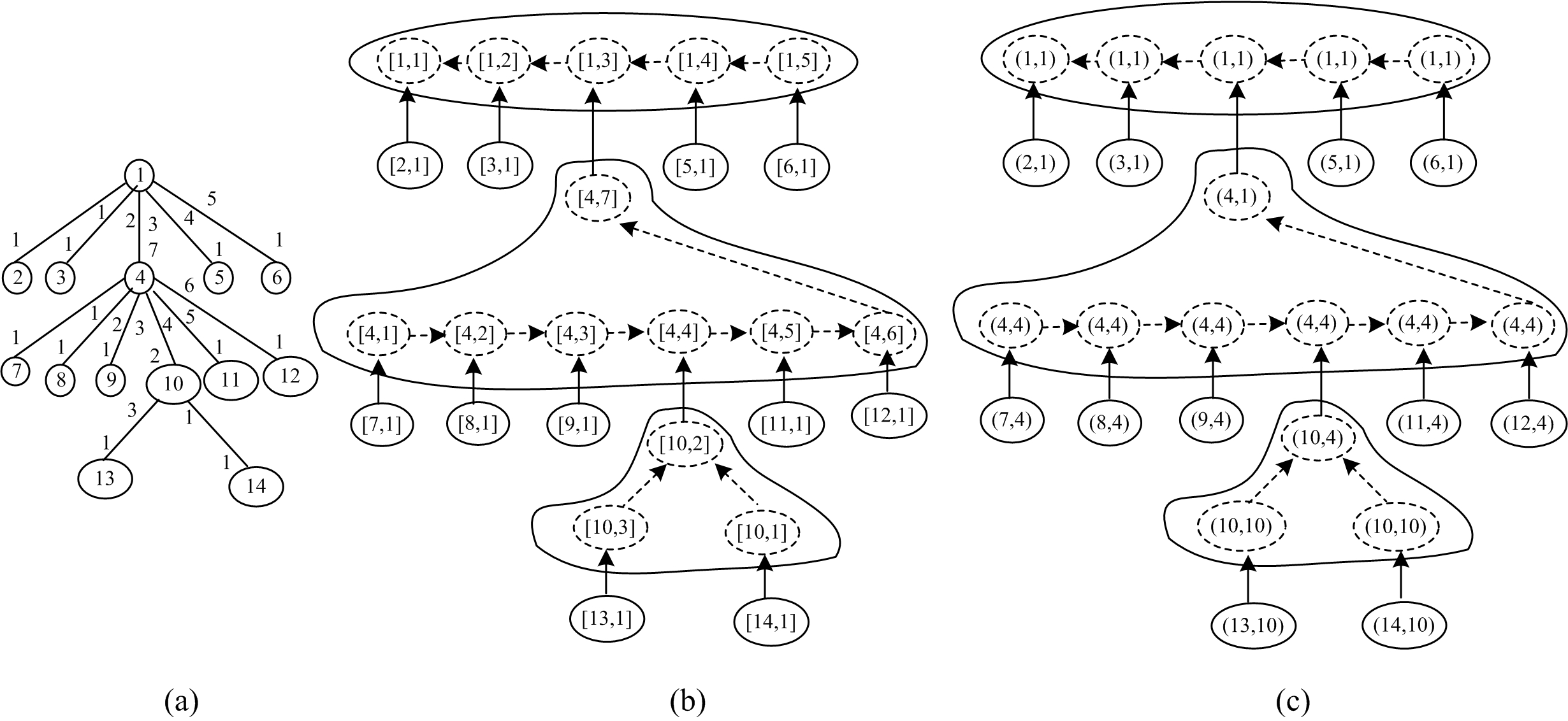
Figure 1: Distributed ordered tree-decomposition of tree network

Using the previous algorithm, we can prove the following.

Theorem 4.1

MSO can be distributively model-checked over tree networks within complexity bounds $TIME=O(\Delta)$ and $MSG/LINK=O(1)$.

5 Planar networks with bounded diameter

We now consider planar networks with bounded diameter, and assume that the diameter $k$ is known by each node. It has been shown that if $G$ is a planar graph with diameter bounded by $k$, then the tree-width of $G$ is bounded by $3k$ [Epp95].

A combinatorial embedding of a planar graph $G=(V,E)$ is an assignment of a cyclic ordering of the set of incident edges to each vertex $v$ such that two edges $(u,v)$ and $(v,w)$ are in the same face iff $(v,w)$ is put immediately before $(v,u)$ in the cyclic ordering of $v$. Combinatorial embeddings, which encode the information about boundaries of the faces in usual embeddings of planar graphs into the planes, are useful for computing on planar graphs. Given a combinatorial embedding, the boundaries of all the faces can be discovered by traversing the edges according to the above condition.

Example 2 (Combinatorial embedding)

The combinatorial embedding and its corresponding usual embedding into the planes are given in resp. Fig.2(a) and Fig.2(b). Suppose the edge $\{a,d\}$ is traversed from $a$ to $d$, then the edge traversed next is $\{d,b\}$, since in the cyclic ordering of $d$, $(d,b)$ is immediately before $(d,a)$. Similarly, the edge traversed after $\{d,b\}$ is $\{b,a\}$.

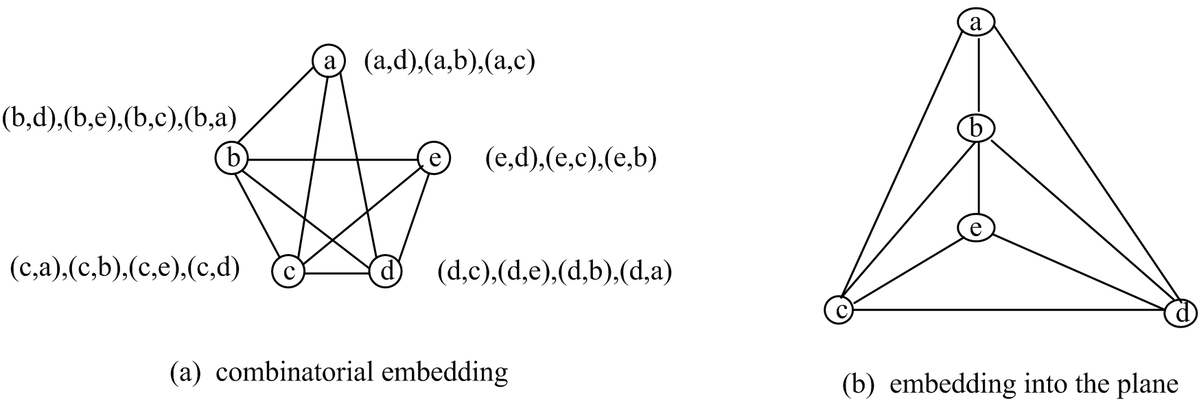
Figure 2: Combinatorial embedding and the corresponding usual embedding into the planes

We assume in this section that a combinatorial embedding of the planar network is distributively stored in the network, i.e. a cyclic ordering of the set of the incident links is stored in each node of the network.

Theorem 5.1

MSO can be distributively model-checked over planar networks with bounded diameter in complexity bounds $TIME=O(n)$ and $MSG/LINK=O(1)$.

The main challenge of Theorem 5.1 is the distributed construction and storage of an ordered tree decomposition. In the following, we explain how to construct distributively an ordered tree decomposition of width $3k$ for a planar network with diameter bounded by $k$ such that the bags of the tree decomposition are stored distributively in the nodes of the network, and for each bag stored in $v$, its parent bag is stored in some neighbor of $v$. If such an ordered tree decomposition has been constructed, it can be transformed into a rooted $\Sigma_{3k}$-labeled binary tree $\mathcal{T}$; the requesting node then transforms the MSO sentence into a bottom-up tree automaton $\mathcal{A}$ and broadcasts it to all the nodes in the network; and $\mathcal{A}$ can be ran distributively over $\mathcal{T}$ in a bottom-up way to check whether $\mathcal{A}$ accepts $\mathcal{T}$ by sending only $O(1)$ messages over each link.

We distinguish whether the planar network is biconnected or not.

5.1 Biconnected planar networks with bounded diameter

In this subsection, we assume that the planar networks are biconnected. It is not hard to verify the following lemma.

Lemma 1

If a planar graph $G$ is biconnected, then the boundaries of all the faces of a combinatorial embedding of $G$ are cycles.

These cycles are called the facial cycles of the combinatorial embedding.

We first recall the centralized construction of a tree decomposition of a biconnected planar graph with bounded diameter [Epp95].

• At first, the biconnected planar graph $G=(V,E)$ is triangulated into a planar graph $G^{\prime}$ by adding edges such that the boundary of each face of $G^{\prime}$, including the outer face, is a triangle;

• A breath-first-search (BFS) tree $T$ of $G^{\prime}$ is constructed;

• An (undirected non-rooted) $2^{V}$-labeled tree $T^{\prime}=(I,F,L)$ is constructed such that

  • $I$ is the set of faces of $G^{\prime}$;

  • $(i_{1},i_{2})\in F$ iff the face $i_{1}$ and $i_{2}$ have a common edge not in the BFS-tree $T$;

  • $L(i)=ancestor(u)\cup ancestor(v)\cup ancestor(w)$, where $\{u,v,w\}$ are exactly the set of vertices contained in face $i$, where $ancestor(x)$ denotes the set of ancestors of $x$ in $T$;

• Finally the tree decomposition is obtained from $T^{\prime}$ by selecting some vertex of $T^{\prime}$, i.e. face of $G^{\prime}$, to which the root of $T$ belongs, as the root, and give directions to the edges of $T^{\prime}$ according to the selected root.

Example 3 (Ordered tree decomposition of biconnected planar graphs with bounded diameter)

A biconnected planar graph $G$ is given in Fig.3(a). The triangulated graph $G^{\prime}$ is in Fig.3(b), with the dashed lines denoting the edges added during the triangulation. A BFS tree of $G^{\prime}$, $T$, is in Fig.3(c), and a constructed ordered tree decomposition $T^{\prime}$ is illustrated in Fig.3(d), with the filled circles denoting the faces (triangles) and arrows between them denoting child-parent relationships. ∎

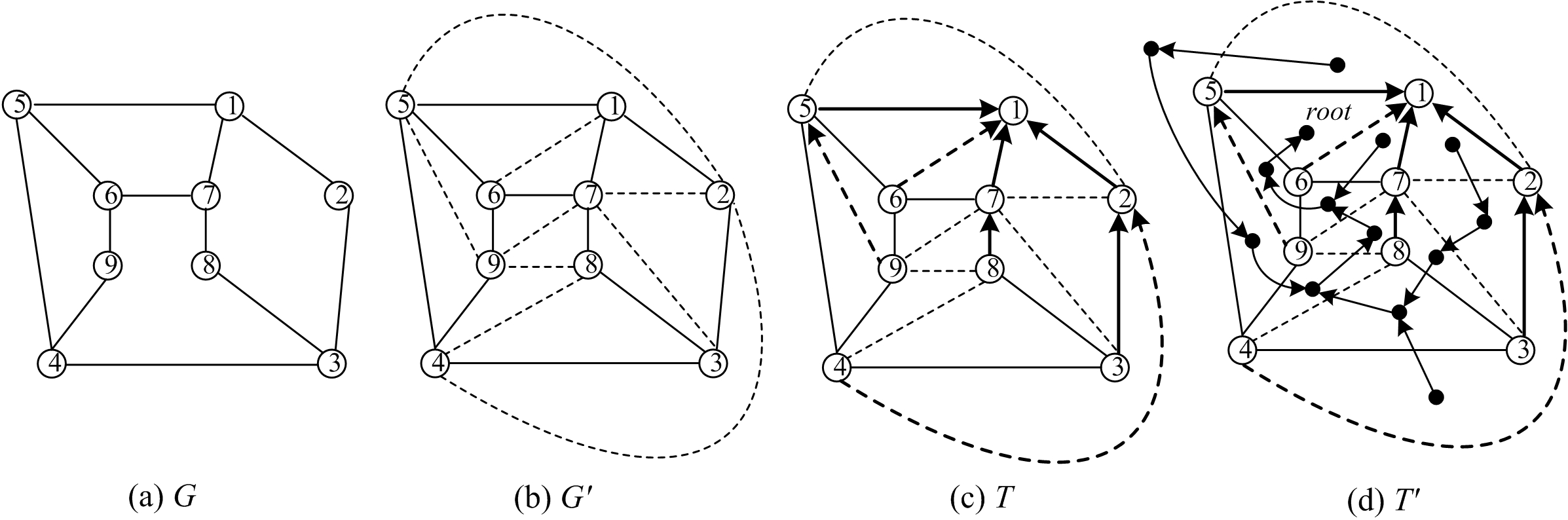
Figure 3: Centralized ordered tree decomposition of biconnected planar graphs with bounded diameter

Our purpose is to transform the above centralized algorithm into a distributed one while satisfying the complexity bound $MSG/LINK=O(1)$. The direct transformation will imply that we should

• first triangulate distributively the planar network,

• then construct distributively a BFS tree for the triangulated network,

• finally construct and store distributively the ordered tree decomposition by using the BFS tree,

while ensuring the complexity bound $MSG/LINK=O(1)$.

Nevertheless, the direct transformation seems infeasible: Even if we can triangulate the biconnected planar network within the complexity bound, it is difficult to construct a BFS tree for the triangulated network with only $O(1)$ messages sent over each link, because the triangulated network includes virtual links between nodes, and two nodes connected by a virtual link may be far away from each other in the real network.

A key observation to tackle this difficulty is that in the above centralized algorithm, a tree decomposition of $G$ can be obtained by using any spanning tree of $G^{\prime}$, not necessarily a BFS tree of it. Thus we can construct a BFS tree of $G$, instead of $G^{\prime}$, which can be done with only $O(1)$ messages sent over each link [BDLP08], and use it to construct the tree decomposition.

The distributed algorithm to construct an ordered tree decomposition for biconnected planar networks with bounded diameter works as follows:

• A BFS-tree of the planar network with the requesting node as the root is distributively constructed and stored;

• A post-order traversal of the BFS-tree can be done, those facial cycles are visited one by one, all the faces in the combinatorial embedding, including the outer face, are triangulated, and the bags corresponding to the triangles are stored among the nodes of the network;

• Finally, some bag stored in the requesting node can be selected as the root bag, and the bags are connected together depending on whether the corresponding triangles share a non-BFS-tree link or not.

We now describe more specifically the post-order traversal of the BFS tree, and how to connect the distributively stored bags into a tree decomposition.

Each link $\{v,w\}$ is seen as two arcs $(v,w)$ and $(w,v)$. Let $l$ be a port of node $v$, then $neighbor(l)$ denotes the neighbor of $v$ corresponding to the port $l$.

Post-order traversal of the BFS tree.

A post-order traversal of the BFS tree is done to visit the nodes one by one.

When a node $v$ is traversed,

If there are arcs $(v,w)$ not visited, let

$$l_{0}:=\min\{l|\exists w\ s.t.\ (v,w)\mbox{ is not visited }\mbox{ and }neighbor(l)=w\}$$

Let $w_{0}=neighbor(l_{0})$, and start traversing the facial cycle which the arc $(v,w_{0})$ belongs to ($(v,w_{0})$ is called the starting arc of the facial cycle, and is seen as the identifier of the facial cycle), by using the cyclic order in each node.

The facial cycle with $(v,w_{0})$ as the starting arc will be triangulated by virtually connecting $v$ to all the non-neighbor nodes of $v$ in the facial cycle. When an arc $(v^{\prime},w^{\prime})$ such that $w^{\prime}\neq v$ and $w^{\prime}\neq w_{0}$ in the facial cycle is visited, the bag (in the ordered tree decomposition) corresponding to the triangle $[v,v^{\prime},w^{\prime}]$ will be stored in $w^{\prime}$. In addition, $w_{0}$ stores the bag $[v,w_{0},w_{1}]$, where $w_{1}$ is the node visited immediately after $w_{0}$ in the facial cycle; and $v$ stores the bag $[v,v^{\ast},w^{\ast}]$, where $v^{\ast}$,$w^{\ast}$ are the last two nodes visited in the facial cycle.

When the traversal of a facial cycle is finished, i.e. $v$ is reached again during the traversal of the facial cycle, then repeat the above procedure until all the arcs $(v,w)$ are visited.

When all the arcs $(v,w)$ have been visited, backtrack to the parent of $v$ in the BFS tree.

Connect the bags into a tree decomposition.

If a bag $[v^{\prime},v^{\prime\prime},v^{\prime\prime\prime}]$ is stored on a node $v$ during the above traversal of a facial cycle, then $[v^{\prime},v^{\prime\prime},v^{\prime\prime\prime}]$ is said to be the bag stored on $v$ corresponding to the facial cycle.

First, select some bag $[v^{\prime},v^{\prime\prime},v^{\prime\prime\prime}]$ stored in the requesting node as the root of the ordered tree decomposition.

Then start visiting the bags stored on the nodes in the facial cycle which has $(v^{\prime},v^{\prime\prime})$ as the starting arc. Now we describe how to visit and connect the bags into a tree decomposition.

Let $(w_{0},\cdots,w_{m})$ be the facial cycle currently visited ($w_{0},w_{m}$ are resp. the first and last visited node during the virtual triangulation process above), and $[v^{\prime}_{0},v^{\prime\prime}_{0},v^{\prime\prime\prime}_{0}]$, $\cdots$, $[v^{\prime}_{m},v^{\prime\prime}_{m},v^{\prime\prime\prime}_{m}]$ be resp. the bags stored on $w_{0},\cdots,w_{m}$ corresponding to the facial cycle.

Suppose $[v^{\prime}_{l},v^{\prime\prime}_{l},v^{\prime\prime\prime}_{l}]$ ($0\leq l\leq m$) is the first visited bag among them during this bag-connecting process.

Let $w_{m+1}=w_{0}$ by convention.

If $l=0$, then the nodes in the facial cycle will be visited according to the order $w_{0}w_{m}\cdots w_{1}$. So $[v^{\prime}_{i+1},v^{\prime\prime}_{i+1},v^{\prime\prime\prime}_{i+1}]$ is taken as the father of $[v^{\prime}_{i},v^{\prime\prime}_{i},v^{\prime\prime\prime}_{i}]$ for all $1\leq i\leq m$ in the tree decomposition.

Note that above we let $[v^{\prime}_{m},v^{\prime\prime}_{m},v^{\prime\prime\prime}_{m}]$ and $[v^{\prime}_{0},v^{\prime\prime}_{0},v^{\prime\prime\prime}_{0}]$ stay together in the tree decomposition because the content of the two bags are in fact the same.

If $l=1$, then the nodes in the facial cycle are visited according to the order $w_{1}\cdots w_{m}w_{0}$. So $[v^{\prime}_{i},v^{\prime\prime}_{i},v^{\prime\prime\prime}_{i}]$ is taken as the father of $[v^{\prime}_{i+1},v^{\prime\prime}_{i+1},v^{\prime\prime\prime}_{i+1}]$ for all $1\leq i\leq m$ in the tree decomposition.

Otherwise ($l>1$), then the nodes in the facial cycle are visited concurrently along the two lines according to the order $w_{l}w_{l+1}\cdots w_{m}w_{0}$ and $w_{l}w_{l-1}\cdots w_{1}$ respectively. So $[v^{\prime}_{i},v^{\prime\prime}_{i},v^{\prime\prime\prime}_{i}]$ is taken as the father of $[v^{\prime}_{i+1},v^{\prime\prime}_{i+1},v^{\prime\prime\prime}_{i+1}]$ for all $l\leq i\leq m$, $[v^{\prime}_{j+1},v^{\prime\prime}_{j+1},v^{\prime\prime\prime}_{j+1}]$ is taken as the father of $[v^{\prime}_{j},v^{\prime\prime}_{j},v^{\prime\prime\prime}_{j}]$ for all $l>j\geq 1$ in the tree decomposition.

Moreover, if during the above process, a node $w_{i+1}$ ($1\leq i\leq m$) is visited through an arc $(w_{i},w_{i+1})$ in the facial cycle, and $\{w_{i},w_{i+1}\}$ is a non-BFS-tree link, then start visiting the new facial cycle which $(w_{i+1},w_{i})$ belongs to; on the other hand, if $w_{i}$ ($i>1$) is visited, and the arc $(w_{i},w_{i-1})$ will be visited next, moreover $\{w_{i},w_{i-1}\}$ is a non-BFS-tree link, then start visiting the new facial cycle which $(w_{i},w_{i-1})$ belongs to.

The detailed distributed algorithm is given in the appendix.

It is not hard to see that only $O(1)$ messages are sent over each link during the computation of the above distributed algorithm. Then we get the following lemma.

Lemma 2

An ordered tree decomposition of biconnected planar networks with bounded diameter can be distributively constructed within the complexity bounds $TIME=O(n)$ and $MSG/LINK=O(1)$.

Example 4 (Distributed ordered tree decomposition of biconnected planar networks with bounded diameter)

A biconnected planar network is given in Fig.4(a) with thick lines denoting the edges of the distributively constructed BFS-tree rooted on the requesting node $1$. The cyclic ordering of each node is the same as the order of the identifiers of the ports. During the post-order traversal of the BFS tree, node $3$ is first traversed, then $2$, $8$, $7$, $6$, $9$, $4$, $5$ and finally $1$. The facial cycles corresponding to face $A$ is visited first, then $B$, $E$, $C$, $D$. The triangulation after the post-order traversal of the BFS-tree is given in Fig.4(b). The constructed tree decomposition is illustrated in Fig.4(c). Note that in Fig.4(c), we only give the distributively stored bags corresponding to face $A$ and $B$, and omit the others in order to avoid overfilling the figure. Suppose the bag $[3,7,1]$ is selected as the root of the tree decomposition, then the child-parent relationship between these distributively stored bags are illustrated in Fig.4(c).

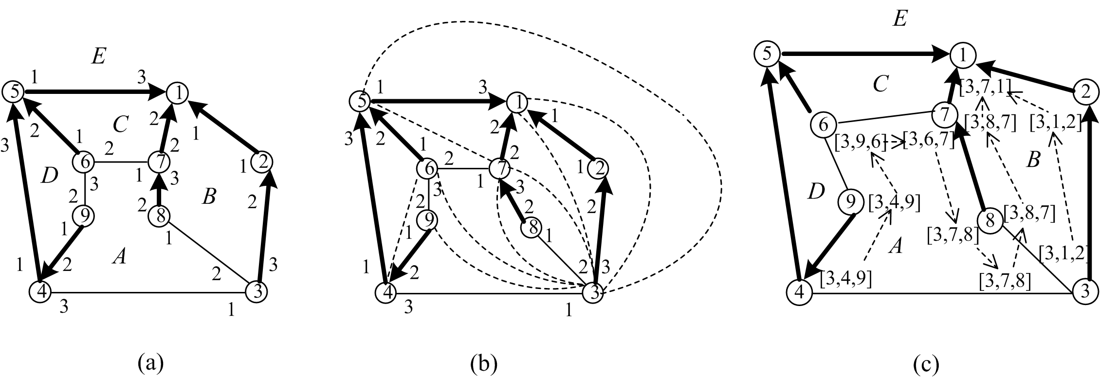
Figure 4: Distributed ordered tree decomposition of biconnected planar networks with bounded diameter

5.2 General planar networks with bounded diameter

Now we consider the general case when the planar networks with bounded diameter are not necessarily biconnected. We first state a proposition on the relationship between the spanning tree of a given graph and the spanning trees of its biconnected components.

Proposition 1

Let $G=(V,E)$ be a connected graph, $T$ a spanning tree of $G$, and $B=(V_{B},E_{B})$ be a nontrivial biconnected component of $G$, then $T[V_{B}]$, the subgraph of $T$ induced by $V_{B}$, is a spanning tree of $B$.

To construct distributively the ordered tree decomposition for (general) planar networks with bounded diameter, we first compute a BFS tree with only $O(1)$ messages sent over each link, and compute distributively the biconnected components of the network by using the algorithm given in [Tur06] within the complexity bounds $TIME=O(n)$ and $MSG/LINK=O(1)$. Then let $T$ be the computed BFS-tree of the network, we compute separately the ordered tree decomposition for each biconnected component $B=(V_{B},E_{B})$ by using $T[V_{B}]$, the subtree of $T$ induced by $V_{B}$. Finally these ordered tree decompositions are connected together into a complete ordered tree decomposition of the whole network.

Lemma 3

The distributed construction of an ordered tree decomposition for (general) planar networks with bounded diameter can be done within the complexity bounds $TIME=O(n)$ and $MSG/LINK=O(1)$.

6 Towards (general) networks with bounded tree width

In the last section, we have shown that MSO can be distributively model-checked over planar networks with bounded diameter with only $O(1)$ messages sent over each link. Courcelle’s classical result states that MSO can be model-checked on graphs with bounded tree width in linear time. Then a natural question to ask is whether we can extend Theorem 5.1 to the (general) networks with bounded tree width.

In the centralized linear-time construction of the tree decomposition, distances between nodes are usually ignored, and two vertices contained in the same bag of the tree decomposition may be far away from each other in the original graph. Thus it seems in general quite difficult, if not impossible, to transform the linear-time centralized tree decomposition algorithm into the distributed one with only a constant number of messages sent over each link. As a matter of fact, distances between vertices in the centralized tree decomposition have been considered in [DG04], where the concept of tree length of a tree decomposition, which is the maximal distance (in the original graph) between vertices in the same bag of a tree decomposition, was defined and investigated.

In this section, based on the work that has been done in [DG04], we consider the distributed model-checking of MSO over networks with bounded degree and bounded tree-length. These classes of networks are of independent interest and they have been applied to construct compact routing schemes for forwarding messages [Dou04]. However, even for these networks, we can only achieve the complexity bound $MSG/LINK=O(1)$ over two more restricted models, namely synchronous distributed systems and asynchronous distributed systems with a BFS tree pre-computed and distributively stored on each node of the network (each node stores locally its parent in the BFS tree). The reason for this restriction on the computational models is in that a BFS tree is essential for the distributed tree decomposition, and currently we do not know how to distributively construct a BFS tree in asynchronous systems with only $O(1)$ messages sent over each link, and the best complexity bound achieved is $MSG/LINK=O(\Delta)$ [BDLP08].

Let $G=(V,E)$ and $X\subseteq V$, then the diameter of $X$ in $G$, denoted $diam_{G}(X)$, is defined by $\max\{dist_{G}(v,w)|v,w\in X\}$. Let $\mathcal{T}=(I,F,r,B)$ be a tree decomposition of $G$, then the length of $\mathcal{T}$, $length(\mathcal{T})$, is defined by $\max\{diam_{G}(B(i))|i\in I\}$. The tree-length of $G$, denoted $tl(G)$, is the minimum length over all tree decompositions of $G$.

Let $\mathcal{C}$ be a class of graphs, we say that $\mathcal{C}$ has bounded tree-length if there is a constant $k$ such that for each $G\in\mathcal{C}$, $tl(G)\leq k$. The following proposition is easy to verify.

Proposition 2

Let $\mathcal{C}$ be a class of networks of bounded degree and bounded tree-length, then $\mathcal{C}$ has bounded tree-width.

In the rest of this subsection, we assume that each node of the network stores locally a bound $d$ on the degree, and a bound $k$ on the tree-length.

Theorem 6.1

MSO can be distributively model-checked over networks with bounded degree and bounded tree-length within the complexity bounds $TIME=O(\Delta)$ and $MSG/LINK=O(1)$, in the following two computational models,

• synchronous distributed systems,

• or asynchronous distributed systems with a BFS tree pre-computed and distributively stored on each node of the network.

The main idea of the proof is to distributively construct an ordered tree decomposition by transforming the BFS-layering tree decomposition algorithm in [DG04]. In the following, we give a more specific description of the construction.

We first recall the centralized construction of the BFS-layering tree decomposition.

Let $s$ be a distinguished vertex in graph $G=(V,E)$. Let $L^{i}=\{v\in V|dist_{G}(s,v)=i\}$. A layering partition of $G$ is a partition of each set $L^{i}$ into $L^{i}_{1},\cdots,L^{i}_{p_{i}}$ such that $u,v\in L^{i}_{j}$ if and only if there exists a path from $u$ to $v$ such that all the intermediate vertices $w$ on the path satisfy that $dist_{G}(s,w)\geq i$.

Let $H=(V_{H},E_{H})$ be the graph defined as follows:

• $V_{H}$: the sets $L^{i}_{j}$.

• $E_{H}$: $\{L^{i}_{j},L^{i^{\prime}}_{j^{\prime}}\}\in E_{H}$ if and only if there is $u\in L^{i}_{j}$ and $v\in L^{i^{\prime}}_{j^{\prime}}$ such that $(u,v)\in E$.

Theorem 6.2

[DG04] The graph $H$ is a tree.

$H$ is called the BFS-layering tree of $G$.

$H$ can be seen as a rooted labeled tree $(I,F,r,B)$ with

• $I=\{(i,j)|L^{i}_{j}\in V_{H}\}$, $F=\{\{(i,j),(i^{\prime},j^{\prime})\}|\{L^{i}_{j},L^{i^{\prime}}_{j^{\prime}}\}\in E_{H}\}$,

• The root $r$ is $(0,1)$,

• $B((i,j))=L^{i}_{j}$.

If we replace the label of $(i,j)$ by $B(i,j)\cup B(i^{\prime},j^{\prime})$ in $H$, where $(i^{\prime},j^{\prime})$ is the parent of $(i,j)$ in $H$, then we get a new rooted labeled tree $\mathcal{S}=(I,F,r,L)$.

Theorem 6.3

[DG04] $\mathcal{S}$ is a tree decomposition of $G$ such that $length(\mathcal{S})\leq 3\cdot tl(G)+1$.

$\mathcal{S}$ is called the BFS-layering tree decomposition of $G$.

Now we transform the above centralized construction into a distributed algorithm in asynchronous distributed systems with a pre-computed BFS tree. The asynchronous distributed algorithm consists of two stages:

Stage 1

: Construct the BFS-layering tree $H$ bottom-up. Because $G$ has bounded tree-length $t$, $\mathcal{S}$ has length no more than $3t+1$ by Theorem 6.3. Thus if two nodes of layer $L^{i}$ are in the same layering partition, then the distance between them is no more than $3t+1$. Consequently, when the layering partition of $L^{i+1}$ has been computed, each node $v$ in $L^{i}$ can know which nodes are in the same layering partition of $L^{i}$ by doing some local computation in its $(3t+1)$-neighborhood.

Stage 2

: Construct the BFS-layering tree decomposition $\mathcal{S}$ from $H$, and an ordered tree decomposition $\mathcal{T}$ from $\mathcal{S}$.

The distributed algorithm to construct the ordered tree decomposition in synchronous systems is similar to the above two-stage algorithm, except that a stage for the BFS-tree construction should be added before the above two stages.

The tree-length of (general) networks with bounded tree-width may be unbounded. The tree-width of a cycle of length $n$ for instance is $2$, while its tree-length is $\lceil n/3\rceil$ [DG04]. For networks of unbounded tree-length, vertices in the same bag of a tree decomposition of the network may be arbitrarily far away from each other. The above technique we use to construct and store the tree decomposition within the complexity bound $MSG/LINK=O(1)$ doesn’t carry over to unbounded tree-length networks, and it seems difficult to extend it.

7 Conclusion

We have seen that MSO sentences can be distributively model-checked over classes of planar networks with bounded diameter, as well as classes of networks with bounded degree and bounded tree-length, with only constant number of messages sent over each link.

So far as the class of graphs on which the results hold is concerned, we doubt that our techniques for MSO can be extended to bounded tree-width graphs, but we were able to prove the result for $k$-outerplanar graphs.

Similar to the centralized computation, the expression complexity for MSO distributed model checking is very high, which hinders the practical value of results obtained in this paper. However, we can relieve the difficulty to some extent by encoding symbolically the tree automata obtained from MSO sentences, in Binary Decision Diagrams (BDD), just like in the MSO model-checker MONA [HJJ⁺96].

Appendix 0.A Step 2 and Step 3 of the linear-time MSO model checking over graphs with bounded tree width

For Step 2, a rooted $\Sigma_{k}$-labeled tree $\mathcal{T}^{\prime}=(T,F,r,\lambda)$, where $\Sigma_{k}=2^{[k+1]^{2}}\times 2^{[k+1]^{2}}\times 2^{[k+1]^{2}}$ ($[k+1]=\{1,2,\cdots,k+1\}$), can be obtained from $\mathcal{T}$ as follows: The new labeling $\lambda$ over $(T,F)$ is defined by $\lambda(t)=(\lambda_{1}(t),\lambda_{2}(t),\lambda_{3}(t))$, where

• $\lambda_{1}(t):=\{(j_{1},j_{2})\in[k+1]^{2}|(b^{t}_{j_{1}},b^{t}_{j_{2}})\in E\}$.

• $\lambda_{2}(t):=\{(j_{1},j_{2})\in[k+1]^{2}|b^{t}_{j_{1}}=b^{t}_{j_{2}}\}$.

• $\lambda_{3}(t):=\left\{\begin{array}[]{cc}\{(j_{1},j_{2})\in[k+1]^{2}|b^{t}_{j_{1}}=b^{t^{\prime}}_{j_{2}}\}&\mbox{for the parent }t^{\prime}\mbox{ of }t,\mbox{ if }t\neq r\\ \emptyset&\mbox{if }t=r\end{array}\right.$

For Step 3, we recall how to translate the MSO sentence $\varphi$ over the vocabulary $\{E\}$ into an MSO sentence $\varphi^{\ast}$ over the vocabulary $\{E_{1},E_{2}\}\cup\{P_{c}|c\in\Sigma_{k}\}$ such that $G\models\varphi$ iff $\mathcal{T}^{\prime}\models\varphi^{\ast}$. The translation relies on the observation that elements and subsets of $V$ can be represented by $(k+1)$-tuples of subsets of $T$. For each element $v\in V$ and $i\in[k+1]$, let

$$U_{i}(v):=\left\{\begin{array}[]{cl}\{t(v)\}&\mbox{, if }b^{t(v)}_{i}=v\mbox{, and }b^{t(v)}_{j}\neq v\mbox{ for all }j:1\leq j<i\\ \emptyset&\mbox{, otherwise}\end{array}\right.$$

where $t(v)$ is the minimal $t\in T$ (with respect to the partial order $\leq^{\mathcal{T}}$) such that $v\in\{b^{t}_{1},\cdots,b^{t}_{k+1}\}$. Let $\overline{U}(v)=(U_{1}(v),\cdots,U_{k+1}(v))$.

For each $S\subseteq V$ and $i\in[k+1]$, let $U_{i}(S):=\cup_{v\in S}U_{i}(v)$, and let $\overline{U}(S)=(U_{1}(S),\cdots,U_{k+1}(S))$. It is not hard to see that for subsets $U_{1},\cdots,U_{k+1}\subseteq T$, there exists $v\in V$ such that $\overline{U}=\overline{U}(v)$ iff

• (1) $\bigcup^{k+1}_{i=1}U_{i}$ is a singleton;

• (2) For all $t\in T$, $i<j<k+1$, if $t\in U_{j}$, then $(i,j)\not\in\lambda_{2}(t)$;

• (3) For all $t\in T$, $i,j<k+1$, if $t\in U_{i}$, then $(i,j)\not\in\lambda_{3}(t)$.

Moreover, there is a subset $S\subseteq V$ such that $\overline{U}=\overline{U}(S)$ iff conditions (2) and (3) are satisfied. Using the above characterizations of $\overline{U}(v)$ and $\overline{U}(S)$, it is easy to construct MSO formulas $Elem(X_{1},\cdots,X_{k+1})$ and $Set(X_{1},\cdots,X_{k+1})$ over $\{E_{1},E_{2}\}\cup\{P_{c}|c\in\Sigma_{k}\}$ such that

$\mathcal{T}^{\prime}\models Elem(\overline{U})\mbox{ iff there is a }v\in V\mbox{ such that }\overline{U}=\overline{U}(v).$

$\mathcal{T}^{\prime}\models Set(\overline{U})\mbox{ iff there is a }S\subseteq V\mbox{ such that }\overline{U}=\overline{U}(S).$

Lemma 4

[FFG02] Every MSO formula $\varphi(X_{1},\cdots,X_{r},y_{1},\cdots,y_{s})$ over vocabulary $E$ can be effectively translated into a formula $\varphi^{\ast}(\overline{X}_{1},\cdots,\overline{X}_{r},\overline{Y}_{1},\cdots,\overline{Y}_{s})$ over the vocabulary $\{E_{1},E_{2}\}\cup\{P_{c}|c\in\Sigma_{k}\}$ such that

(1) For all $S_{1},\cdots,S_{r}\subseteq V$, and $v_{1},\cdots,v_{s}\in V$,

$$G\models\varphi(S_{1},\cdots,S_{r},v_{1},\cdots,v_{s})\mbox{ iff }\mathcal{T}^{\prime}\models\varphi^{\ast}(\overline{U}(S_{1}),\cdots,\overline{U}(S_{r}),\overline{U}(v_{1}),\cdots,\overline{U}(v_{s})).$$

(2) For all $\overline{U}_{1},\cdots,\overline{U}_{r},\overline{W}_{1},\cdots,\overline{W}_{s}\subseteq T$ such that $\mathcal{T}^{\prime}\models\varphi^{\ast}(\overline{U}_{1},\cdots,\overline{U}_{r},\overline{W}_{1},$ $\cdots,\overline{W}_{s})$, there exist $S_{1},\cdots,S_{r}\subseteq V$, $v_{1},\cdots,v_{s}\in V$ such that $\overline{U}_{i}=\overline{U}(S_{i})$ for all $1\leq i\leq r$ and $\overline{W}_{j}=\overline{U}(v_{j})$ for all $1\leq j\leq s$.

Appendix 0.B Distributed model-checking of MSO over tree networks

Suppose each node stores the states of ports, “parent” or “child”, with respect to the rooted tree (with the requesting node as the root).

Through local replacement of each node $v$ by the set of (virtual) nodes $\{[v,i]|1\leq i\leq deg(v)\}$, the network is first transformed into a (virtual) binary tree, then an ordered tree decomposition $\mathcal{T}$ of width $1$ and rank $\leq 2$ is obtained;

The tree decomposition $\mathcal{T}$ is transformed into a $\Sigma_{2}$-labeled binary tree $\mathcal{T}^{\prime}$;

The requesting node constructs a tree automata $\mathcal{A}$ from $\varphi$, and broadcasts $\mathcal{A}$ to all the nodes in the network;

Finally $\mathcal{A}$ is ran distributively over $\mathcal{T}^{\prime}$ in a bottom-up way to decide whether $\mathcal{T}^{\prime}$ is accepted by $\mathcal{A}$.

In the following we describe the distributed algorithm in detail by giving the pseudo-code for the message processing at each node $v$.

Initialization

The requesting node $v_{0}$ sets $Virtual(v_{0}):=\langle[v_{0},1],[v_{0},2],\dots,[v_{0},deg(v_{0})]\rangle$.

The requesting node sends message START over all its ports.

Message START over port $l$

$Virtual(v):=\langle[v,1],[v,2],\dots,[v,deg(v)]\rangle$.

if $deg(v)>1$ then

$v$ sends message START over all ports $l^{\prime}$ such that $state(l^{\prime})=$“child”.

else

$v$ sends message ACK over port $l$.

end if

Message ACK over port $l$

$bAck(l):=true$.

if $bAck(l^{\prime})=true$ for each port $l^{\prime}$ such that $state(l^{\prime})=$“child” then

if $v$ is the requesting node then

$v$ sends message TREEDECOMP over all its ports.

else

$v$ sends message ACK over the port $l^{\prime}$ such that $state(l^{\prime})=$“parent”.

end if

end if

Message TREEDECOMP over port $l$

$Bag([v,l]):=(v,parent(v))$. for each $l^{\prime}:1\leq l^{\prime}\leq deg(v),l^{\prime}\neq l$ do

$Bag([v,l^{\prime}]):=(v,v)$.

end for

if $deg(v)=1$ then

$v$ sends message DECOMPOVER over the port $l^{\prime}$ such that $state(l^{\prime})=$“parent”.

else

$v$ sends message TREEDECOMP over all ports $l^{\prime}$ such that $state(l^{\prime})=$“child”.

end if

Message DECOMPOVER over port $l$

$bDecompOver(l):=true$.

if $bDecompOver(l^{\prime})=true$ for each port $l^{\prime}$ such that $state(l^{\prime})=$“child” then

if $v$ is the requesting node then

for each $l^{\prime}$ do

$\lambda_{1}([v,l^{\prime}]):=\emptyset$, $\lambda_{2}([v,l^{\prime}]):=\{(1,2),(2,1)\}$, $\lambda_{3}([v,l^{\prime}]):=\emptyset$, $\lambda([v,l^{\prime}]):=(\lambda_{1}([v,l^{\prime}]),\lambda_{2}([v,l^{\prime}]),\lambda_{3}([v,l^{\prime}]))$.

$v$ sends message TREELABELING over port $l^{\prime}$.

end for

else

$v$ sends message DECOMPOVER over the port $l^{\prime}$ such that $state(l^{\prime})=$“parent”.

end if

end if

Message TREELABELING over port $l$

$\lambda_{1}([v,l]):=\{(1,2),(2,1)\}$, $\lambda_{2}([v,l]):=\emptyset$, $\lambda_{3}([v,l]):=\{(2,1),(2,2)\}$, $\lambda([v,l]):=(\lambda_{1}([v,l]),\lambda_{2}([v,l]),\lambda_{3}([v,l]))$.

for each $l^{\prime}:1\leq l^{\prime}\leq deg(v),l^{\prime}\neq l$ do

$\lambda_{1}([v,l^{\prime}]):=\emptyset$, $\lambda_{2}([v,l^{\prime}]):=\{(1,2),(2,1)\}$.

end for

if $deg(v)>1$ then

if $l=1$ then

$\lambda_{3}([v,2]):=\{(1,1),(2,1)\}$, $\lambda([v,2]):=(\lambda_{1}([v,2]),\lambda_{2}([v,2]),\lambda_{3}([v,2]))$.

for each $l^{\prime}:3\leq l^{\prime}\leq deg(v)$ do

$\lambda_{3}([v,l^{\prime}]):=\{(1,1),(1,2),(2,1),(2,2)\}$, $\lambda([v,l^{\prime}]):=(\lambda_{1}([v,l^{\prime}]),\lambda_{2}([v,l^{\prime}]),\lambda_{3}([v,l^{\prime}]))$.

end for

else if $l=deg(v)$ then

$\lambda_{3}([v,deg(v)-1]):=\{(1,1),(2,1)\}$.

$\lambda([v,deg(v)-1]):=(\lambda_{1}([v,deg(v)-1]),\lambda_{2}([v,deg(v)-1]),\lambda_{3}([v,deg(v)-1]))$.

for each $l^{\prime}:1\leq l^{\prime}\leq deg(v)-2$ do

$\lambda_{3}([v,l^{\prime}]):=\{(1,1),(1,2),(2,1),(2,2)\}$, $\lambda([v,l^{\prime}]):=(\lambda_{1}([v,l^{\prime}]),\lambda_{2}([v,l^{\prime}]),\lambda_{3}([v,l^{\prime}]))$.

end for

else

$\lambda_{3}([v,l-1]):=\lambda_{3}([v,l+1]):=\{(1,1),(2,1)\}$.

$\lambda([v,l-1]):=(\lambda_{1}([v,l-1]),\lambda_{2}([v,l-1]),\lambda_{3}([v,l-1]))$.

$\lambda([v,l+1]):=(\lambda_{1}([v,l+1]),\lambda_{2}([v,l+1]),\lambda_{3}([v,l+1]))$.

for each $l^{\prime}:1\leq l^{\prime}\leq deg(v),l^{\prime}\neq l-1,l,l+1$ do

$\lambda_{3}([v,l^{\prime}]):=\{(1,1),(1,2),(2,1),(2,2)\}$, $\lambda([v,l^{\prime}]):=(\lambda_{1}([v,l^{\prime}]),\lambda_{2}([v,l^{\prime}]),\lambda_{3}([v,l^{\prime}]))$.

end for

end if

$v$ sends message TREELABELING over each port $l^{\prime}$ such that $state(l^{\prime})=$“child”.

else

$v$ sends message LABELINGOVER over the port $l^{\prime}$ such that $state(l^{\prime})=$“parent”.

end if

Message LABELINGOVER over port $l$

$bLabelingOver(l):=true$.

if $bLabelingOver(l^{\prime})=true$ for each port $l^{\prime}$ such that $state(l^{\prime})=$“child” then

if $v$ is the requesting node then

$v$ constructs tree automaton $\mathcal{A}=(Q,\Sigma_{2},\delta,f_{0},F)$ from $\varphi$.

$v$ sends message AUTOMATON($\mathcal{A}$) over all its ports.

else

$v$ sends message LABELINGOVER over the port $l^{\prime}$ such that $state(l^{\prime})=$“parent”.

end if

end if

Message AUTOMATON($\mathcal{A}$) over port $l$

Let $\mathcal{A}=(Q,\Sigma_{2},\delta,f_{0},F)$.

$automaton(v):=(Q,\Sigma_{2},\delta,f_{0},F)$.

if $deg(v)=1$ then

$v$ sends message STATE($f_{0}(\lambda([v,1]))$) over the port $l^{\prime}$ such that $state(l^{\prime})=$“parent”.

else

$v$ sends message AUTOMATON($\mathcal{A}$) over all ports $l^{\prime}$ such that $state(l^{\prime})=$“child”.

end if

Message STATE($q$) over port $l$

$bState(l):=true$, $childState(l):=q$.

if $bState(l^{\prime})=true$ for each port $l^{\prime}$ such that $state(l^{\prime})=$“child” then

if $v$ is the requesting node then

$state([v,deg(v)]):=\delta(childState(deg(v)),\lambda([v,deg(v)]))$.

for $l^{\prime}$ from $deg(v)-1$ to $1$ do

$state([v,l^{\prime}]):=\delta(childState(l^{\prime}),state([v,l^{\prime}+1]),\lambda([v,l^{\prime}]))$.

end for

if $state([v,1])\in F$ then $result(\varphi):=true$.

else $result(\varphi):=false$.

end if

else

Let $l_{0}$ be the port with state “parent”.

if $l_{0}=1$ then

$state([v,deg(v)]):=\delta(childState(deg(v)),\lambda([v,deg(v)]))$.

for $l^{\prime}$ from $deg(v)-1$ to $2$ do

$state([v,l^{\prime}]):=\delta(childState(l^{\prime}),state([v,l^{\prime}+1]),\lambda([v,l^{\prime}]))$.

end for

$state([v,1]):=\delta(state([v,2]),\lambda([v,1]))$.

else if $l_{0}=deg(v)$ then

$state([v,1]):=\delta(childState(1),\lambda([v,1]))$.

for $l^{\prime}$ from $2$ to $deg(v)-1$ do

$state([v,l^{\prime}]):=\delta(state([v,l^{\prime}-1]),childState(l^{\prime}),\lambda([v,l^{\prime}]))$.

end for

$state([v,deg(v)]):=\delta(state([v,deg(v)-1]),\lambda([v,deg(v)]))$.

else

$state([v,1]):=\delta(childState(1),\lambda([v,1]))$.

$state([v,deg(v)]):=\delta(childState(deg(v)),\lambda([v,deg(v)]))$.

for $l^{\prime}$ from $2$ to $l_{0}-1$ do

$state([v,l^{\prime}]):=\delta(state([v,l^{\prime}-1]),childState(l^{\prime}),\lambda([v,l^{\prime}]))$.

end for

for $l^{\prime}$ from $deg(v)-1$ to $l_{0}+1$ do

$state([v,l^{\prime}]):=\delta(childState(l^{\prime}),state([v,l^{\prime}+1]),\lambda([v,l^{\prime}]))$.

end for

$state([v,l_{0}]):=\delta(state([v,l_{0}-1]),state([v,l_{0}+1]),\lambda([v,l_{0}]))$.

end if

$v$ sends message STATE($state([v,l_{0}])$) over port $l_{0}$.

end if

end if

Appendix 0.C Distributed ordered tree decomposition of biconnected planar networks with bounded diameter

First, a breadth-first-search (BFS) tree rooted on the requesting node is distributively constructed and stored in the network such that each node $v$ stores the identifier of its parent in the BFS-tree ($parent(v)$), and the states of the ports with respect to the BFS-tree ($state(l)$ for each port $l$), which are either “parent”, or “child”, or “non-tree” [BDLP08].

Then, the requesting node sends messages to ask each node $v$ to get the list of all its ancestors, denoted as $ancestor(v)$, and all its neighbors ($neighbor(l)$ for each port $l$) within the complexity bounds.

By a post-order traversal of the BFS-tree, $G$ can be triangulated as follows. Each bidirectional link is seen as two arcs with reverse directions. When traversing a node $v$, if all the arcs (starting from $v$) $(v,w)$ have been traversed, then backtrack to the parent of $v$ and traverse the next node; otherwise, for each arc $(v,w)$ that has not been traversed before, walk along the facial cycle containing $(v,w)$ according to the cyclic ordering in each node and $(v,w)$ is called the starting arc of this facial cycle. When all the walks of those facial cycles returned to $v$, then backtrack to the parent of $v$ and traverse the next node. When an arc $(v^{\prime},w^{\prime})$ in a facial cycle is traversed, let $(v_{0},w_{0})$ be the starting arc of the facial cycle, we imagine that $v^{\prime}$ and $w^{\prime}$ are connected by virtual edges to $v_{0}$, i.e. imagine $\{v_{0},v^{\prime},w^{\prime}\}$ as a triangle in the triangulated graph, then the node $w^{\prime}$ stores locally the starting arc $(v_{0},w_{0})$ and the information about the bag corresponding to the triangle $\{v_{0},v^{\prime},w^{\prime}\}$.

After $G$ is triangulated, an ordered tree decomposition can be obtained by selecting some bag stored in the requesting node as the root bag, and connecting together all the bags (corresponding to the triangles) depending on whether they share a non-BFS-tree link or not.

In the following, we describe the distributed algorithm in detail by giving the pseudo-code for the message processing at each node $v$.

Initialization

The requesting node sends messages to ask each node to

get the list of its ancestors in the BFS-tree and all its neighbors.

For each node $v$, let $ancestor(v)$ be the list of its ancestors.

For each port $l$, let $neighbor(l)$ be the neighbor connected to $l$.

The requesting node sets $traversed(1):=true$, and sends POSTTRAVERSE over port $1$.

Message POSTTRAVERSE over port $l$

if $v$ is a leaf in the BFS-tree then

if there exist $l^{\prime}$ such that $arcVisited(v,neighbor(l^{\prime}))=false$ then

for each $l^{\prime}:arcVisited(v,neighbor(l^{\prime}))=false$ do

$arcVisited(v,neighbor(l^{\prime})):=true$.

$v$ sends FACESTART(($v$,$neighbor(l^{\prime})$), $ancestor(v)$, $ancestor(v)$) over $l^{\prime}$.

end for

else

$v$ sends BACKTRACK over the port $l^{\prime}$ such that $state(l^{\prime})=$“parent”.

end if

else

Let $l^{\prime}$ be the minimal port such that $state(l^{\prime})=$“child”.

$v$ sets $traversed(l^{\prime}):=true$ and sends message POSTTRAVERSE over $l^{\prime}$.

end if

Message FACESTART(($u_{1}$,$u_{2}$), $(w_{1},\cdots,w_{r})$, $(w^{\prime}_{1},\cdots,w^{\prime}_{s})$) over the port $l$

$arcVisited(neighbor(l),v):=true$.

Let $l^{\prime}$ be the port such that $(v,neighbor(l^{\prime}))$ is immediately before $(v,neighbor(l))$ in the cyclic ordering.

if $v=u_{2}$ then

$v$ sends message FACESTART(($u_{1}$,$u_{2}$),$(w_{1},\cdots,w_{r})$, $ancestor(v)$) over port $l^{\prime}$.

else

$Bag(u_{1},neighbor(l),v):=\langle(u_{1},u_{2}),list_{3k+1}((w_{1},\cdots,w_{r})\cdot(w^{\prime}_{1},\cdots,w^{\prime}_{s})\cdot ancestor(v))\rangle$.

% $list_{3k+1}(w_{1},\cdots,w_{p})$ ($p\leq 3k+1$) generates a list of length $3k+1$

from $w_{1},\cdots,w_{p}$ by repeating $w_{p}$ after $w_{1},\cdots,w_{p}$.

$v$ sends message ACKFACESTART(($u_{1}$,$u_{2}$), $(w_{1},\cdots,w_{r})$, $ancestor(v)$) over port $l$.

if $neighbor(l^{\prime})=u_{1}$ then    % $\{u_{1},u_{2},v\}$ is a triangle.

$v$ sends message FACEOVER(($u_{1}$,$u_{2}$), $neighbor(l)$, $(w^{\prime}_{1},\cdots,w^{\prime}_{s})$, $ancestor(v)$) over port $l^{\prime}$.

else

$v$ sends message FACEWALK(($u_{1}$,$u_{2}$), $(w_{1},\cdots,w_{r})$, $ancestor(v)$) over port $l^{\prime}$.

end if

$arcVisited(v,neighbor(l^{\prime})):=true$.

end if

Message ACKFACESTART(($u_{1}$,$u_{2}$), $(w_{1},\cdots,w_{r})$, $(w^{\prime}_{1},\cdots,w^{\prime}_{s})$) over port $l$

$Bag(u_{1},v,neighbor(l)):=\langle(u_{1},u_{2}),list_{3k+1}((w_{1},\cdots,w_{r})\cdot ancestor(v)\cdot(w^{\prime}_{1},\cdots,w^{\prime}_{s}))\rangle$.

Message FACEOVER(($u_{1}$,$u_{2}$), $v^{\prime}$, $(w_{1},\cdots,w_{r})$, $(w^{\prime}_{1},\cdots,w^{\prime}_{s})$) over port $l$

$arcVisited(neighbor(l),v):=true$.

$Bag(v,v^{\prime},neighbor(l)):=\langle(u_{1},u_{2}),list_{3k+1}(ancestor(v)\cdot(w_{1},\cdots,w_{r})\cdot(w^{\prime}_{1},\cdots,w^{\prime}_{s}))\rangle$.

if $arcVisited(neighbor(l^{\prime}),v)=true$ for each $l^{\prime}$ then

if $v$ is the requesting node then

$root:=(v,v^{\prime},neighbor(l))$, $bLeafBag(v,v^{\prime},neighbor(l)):=false$.

$v$ sends message ANTIBAGVISIT($(v,v^{\prime},neighbor(l))$,$Bag(v,v^{\prime},neighbor(l))$) over port $l$.

else

$v$ sends message BACKTRACK over link $l^{\prime}$ such that $state(l^{\prime})=$“parent”.

end if

end if

Message FACEWALK(($u_{1}$,$u_{2}$), $(w_{1},\cdots,w_{r})$, $(w^{\prime}_{1},\cdots,w^{\prime}_{s})$) over port $l$

$arcVisited(neighbor(l),v):=true$.

$Bag(u_{1},neighbor(l),v):=\langle(u_{1},u_{2}),list_{3k+1}((w_{1},\cdots,w_{r})\cdot(w^{\prime}_{1},\cdots,w^{\prime}_{s})\cdot ancestor(v))\rangle$.

Let $l^{\prime}$ be the port such that

$(v,neighbor(l^{\prime}))$ is immediately before $(v,neighbor(l))$ in the cyclic ordering.

if $neighbor(l^{\prime})=u_{1}$ then

$v$ sends message FACEOVER(($u_{1}$,$u_{2}$),$(w^{\prime}_{1},\cdots,w^{\prime}_{s})$, $ancestor(v)$) over port $l^{\prime}$.

else

$v$ sends message FACEWALK(($u_{1}$,$u_{2}$),$(w_{1},\cdots,w_{r})$, $ancestor(v)$) over port $l^{\prime}$.

end if

$arcVisited(v,neighbor(l^{\prime})):=true$.

Message BACKTRACK over port $l$

if there exists $l^{\prime}$ such that $state(l^{\prime})=$“child” and $traversed(l^{\prime})=false$ then

Let $l^{\prime}$ be the minimal port such that $state(l^{\prime})=$“child” and $traversed(l^{\prime})=false$.

$v$ sets $traversed(l^{\prime}):=true$ and sends POSTTRAVERSE over $l^{\prime}$.

else if there exists $l^{\prime}$ such that $arcVisited(v,neighbor(l^{\prime}))=false$ then

for each port $l^{\prime}$ such that $arcVisited(v,neighbor(l^{\prime}))=false$ do

$arcVisited(v,neighbor(l^{\prime})):=true$.

$v$ sends FACESTART(($v$,$neighbor(l^{\prime})$),$ancestor(v)$, $ancestor(v)$) over port $l^{\prime}$.

end for

else

% All the children of $v$ have been traversed and all the facial cycles containing $v$ have been visited.

if $v$ is not the requesting node then

$v$ sends message BACKTRACK over the port $l^{\prime}$ such that $state(l^{\prime})=$“parent”.

else

$v$ selects some bag $(v^{\prime},v^{\prime\prime},v^{\prime\prime\prime})$ stored in it.

$root:=(v^{\prime},v^{\prime\prime},v^{\prime\prime\prime})$, $bLeafBag(v^{\prime},v^{\prime\prime},v^{\prime\prime\prime}):=false$.

if $v=v^{\prime}$ then

% $(v^{\prime\prime\prime},v)$ is the last arc of the facial cycle.

Let $l^{\prime}$ be the port such that $neighbor(l^{\prime})=v^{\prime\prime\prime}$.

$v$ sends message ANTIBAGVISIT($(v,v^{\prime\prime},v^{\prime\prime\prime})$, $Bag(v,v^{\prime\prime},v^{\prime\prime\prime})$) over port $l^{\prime}$.

if $state(l^{\prime})=$“non-tree” then

% $(v^{\prime\prime\prime},v)$ is the last arc of the facial cycle.

$v$ sends message NEWFACEBAG($(v,v^{\prime\prime},v^{\prime\prime\prime})$, $Bag(v,v^{\prime\prime},v^{\prime\prime\prime})$) over port $l^{\prime}$.

end if

else if $v=v^{\prime\prime}$ then

% $(v,v^{\prime\prime})$ is the starting arc of the facial cycle.

Let $l^{\prime}$ be the port such that $neighbor(l^{\prime})=v^{\prime}$.

Let $l^{\prime\prime}$ be the port such that $neighbor(l^{\prime\prime})=v^{\prime\prime\prime}$.

$v$ sends message BAGVISIT($(v^{\prime},v,v^{\prime\prime\prime})$, $Bag(v^{\prime},v,v^{\prime\prime\prime})$) over port $l^{\prime\prime}$.

if $state(l^{\prime})=$“non-tree” then

$v$ sends message NEWFACEBAG($(v^{\prime},v,v^{\prime\prime\prime})$, $Bag(v^{\prime},v,v^{\prime\prime\prime})$) over port $l^{\prime}$.

end if

else

% $v=v^{\prime\prime\prime}$.

Let $l^{\prime}$ be the port such that $neighbor(l^{\prime})=v^{\prime\prime}$.

Let $l^{\prime\prime}$ be the port such that $(v,neighbor(l^{\prime\prime}))$ is immediately before $(v,v^{\prime\prime})$ in the cyclic ordering.

$v$ sends message ANTIBAGVISIT($(v^{\prime},v^{\prime\prime},v)$, $Bag(v^{\prime},v^{\prime\prime},v)$) over port $l^{\prime}$.

if $state(l^{\prime})=$“non-tree” then

$v$ sends message NEWFACEBAG($(v^{\prime},v^{\prime\prime},v)$, $Bag(v^{\prime},v^{\prime\prime},v)$) over port $l^{\prime}$.

end if

$v$ sends message BAGVISIT($(v^{\prime},v^{\prime\prime},v)$, $Bag(v^{\prime},v^{\prime\prime},v)$) over port $l^{\prime\prime}$.

end if

end if

end if

Message BAGVISIT($bagId$, $bag$) over port $l$

Let $bagId:=(w_{1},w_{2},w_{3})$, $bag:=\langle(u_{1},u_{2}),(w^{\prime}_{1},\cdots,w^{\prime}_{3k+1})\rangle$.

if $v=u_{1}$ then

Let $(v,v^{\prime},v^{\prime\prime})$ be the stored bag such that $Bag(v,v^{\prime},v^{\prime\prime})=\langle(u_{1},u_{2}),(\cdots)\rangle$.

$father(v,v^{\prime},v^{\prime\prime}):=(bagId,bag)$.

if $state(l)=$“non-tree” then

$v$ sends message NEWFACEBAG$((v,v^{\prime},v^{\prime\prime}),Bag(v,v^{\prime},v^{\prime\prime}))$ over port $l$.

else $bLeafBag(v,v^{\prime},v^{\prime\prime}):=true$.

end if

else

$father(u_{1},neighbor(l),v):=(bagId,bag)$, $bLeafBag(u_{1},neighbor(l),v):=false$.

if $state(l)=$“non-tree” then

$v$ sends message NEWFACEBAG$((u_{1},neighbor(l),v),Bag(u_{1},neighbor(l),v))$ over port $l$.

end if

Let $l^{\prime}$ be the port such that $(v,neighbor(l^{\prime}))$ is immediately before $(v,neighbor(l))$ in the cyclic ordering.

$v$ sends message BAGVISIT($(u_{1},neighbor(l),v)$,$Bag(u_{1},neighbor(l),v)$) over port $l^{\prime}$.

end if

Message ANTIBAGVISIT($bagId$, $bag$) over port $l$

Let $bagId:=(w_{1},w_{2},w_{3})$, $bag:=\langle(u_{1},u_{2}),(w^{\prime}_{1},\cdots,w^{\prime}_{3k+1})\rangle$.

Let $l^{\prime}$ be the port such that $(v,neighbor(l))$ is immediately before $(v,neighbor(l^{\prime}))$ in the cyclic ordering.

if $neighbor(l^{\prime})=u_{1}$ then

if $state(l^{\prime})=$“non-tree” then

$bLeafBag(u_{1},v,neighbor(l)):=false$.

$v$ sends NEWFACEBAG($(u_{1},v,neighbor(l)),Bag(u_{1},v,neighbor(l))$) over $l^{\prime}$.

else $bLeafBag(u_{1},v,neighbor(l)):=true$.

end if

else

$father(u_{1},neighbor(l^{\prime}),v):=(bagId,bag)$, $bLeafBag(u_{1},neighbor(l^{\prime}),v):=false$.

$v$ sends message ANTIBAGVISIT$((u_{1},neighbor(l^{\prime}),v),Bag(u_{1},neighbor(l^{\prime}),v))$ over $l^{\prime}$.

if $state(l^{\prime})=$“non-tree” then

$v$ sends message NEWFACEBAG$((u_{1},neighbor(l^{\prime}),v),Bag(u_{1},neighbor(l^{\prime}),v))$ over port $l^{\prime}$.

end if

end if

Message NEWFACEBAG($bagId$,$bag$) over port $l$

Let $(v^{\prime},v^{\prime\prime},v^{\prime\prime\prime})$ be the stored bag such that $(neighbor(l),v)=(v^{\prime},v^{\prime\prime})$ or $(v^{\prime\prime},v^{\prime\prime\prime})$ or $(v^{\prime\prime\prime},v^{\prime})$.

% $(neighbor(l),v)=(v^{\prime},v^{\prime\prime})$: $(neighbor(l),v)$ is the first arc traversed in the new facial cycle.

% $(neighbor(l),v)=(v^{\prime\prime\prime},v^{\prime})$: $(neighbor(l),v)$ is the last arc traversed in the new facial cycle.

$father(v^{\prime},v^{\prime\prime},v^{\prime\prime\prime}):=(bagId,bag)$, $bLeafBag(v^{\prime},v^{\prime\prime},v^{\prime\prime\prime}):=false$.

if $(neighbor(l),v)=(v^{\prime},v^{\prime\prime})$ then

Let $l^{\prime}$ be the port such that $neighbor(l^{\prime})=v^{\prime\prime\prime}$.

$v$ sends message BAGVISIT($(v^{\prime},v,v^{\prime\prime\prime})$, $Bag(v^{\prime},v,v^{\prime\prime\prime})$) over port $l^{\prime}$.

else if $(neighbor(l),v)=(v^{\prime\prime\prime},v^{\prime})$ then

$v$ sends message ANTIBAGVISIT($(v,v^{\prime\prime},v^{\prime\prime\prime})$, $Bag(v,v^{\prime\prime},v^{\prime\prime\prime})$) over port $l$.

else

Let $l^{\prime}$ be the port such that $(v,neighbor(l^{\prime}))$ is immediately before $(v,neighbor(l))$ in the cyclic ordering.

$v$ sends message ANTIBAGVISIT($(v^{\prime},v^{\prime\prime},v)$, $Bag(v^{\prime},v^{\prime\prime},v)$) over port $l$.

$v$ sends message BAGVISIT($(v^{\prime},v^{\prime\prime},v)$, $Bag(v^{\prime},v^{\prime\prime},v)$) over port $l^{\prime}$.

end if

Appendix 0.D Distributed ordered tree decomposition of general planar networks with bounded diameter

First, a breadth-first-search (BFS) tree rooted on the requesting node is distributively constructed and stored in the network such that each node $v$ stores the identifier of its parent in the BFS-tree ($parent(v)$), and the states of the ports with respect to the BFS-tree ($state(l)$ for each port $l$), which are either “parent”, or “child”, or “non-tree” [BDLP08].

Then, a distributed depth-first-search can be done to decompose the planar network with bounded diameter into biconnected components (also called blocks) [Tur06]. An ordered tree decomposition for each block is constructed. Finally these ordered tree decompositions are connected together to get the complete tree decomposition of the whole network.

We first describe the distributed algorithm to decompose the network into blocks by giving the pseudo-code for the message processing at each node $v$.

Initialization

The requesting node $v_{0}$ sets $DFSDepth(v_{0}):=DFSLow(v_{0}):=0$, $DFSVisited(v_{0}):=false$.

The requesting node $v_{0}$ sets $DFSState(l):=$“unvisited” for each port $l$.

The requesting node sets $DFSState(1):=$“child” and sends message FORWARD($1$,$0$) over port $1$.

Message FORWARD($nextBlockId$, $parentDepth$) over port $l$

if $DFSVisited(v)=false$ then

$DFSVisited(v):=true$, $DFSState(l):=$“parent”, $DFSState(l^{\prime}):=$“unvisited” for each port $l^{\prime}\neq l$.

$DFSDepth(v):=parentDepth+1$, $DFSLow(v):=DFSDepth(v)$.

if $v$ has at least two ports then

Let $l^{\prime}$ be the minimal port such that $l^{\prime}\neq l$.

$DFSState(l^{\prime}):=$“child”, $v$ sends message FORWARD($nextBlockId$, $DFSDepth(v)$) over $l^{\prime}$.

else $v$ sends message BACKTRACK($nextBlockId$,$DFSLow(v)$) and message BLOCKACK over $l$.

end if

else $DFSState(l):=$“non-tree-forward”, $v$ sends message RESTART$(nextBlockId,DFSDepth(v))$ over $l$.

end if

Message BACKTRACK($nextBlockId$, $childLow$) over port $l$

if $childLow>=DFSDepth(v)$ then

$articulation(v):=true$.

if $childLow=DFSDepth(v)$ then

$DFSState(l):=$“closed”, $blockIds:=blockIds\cup\{nextBlockId\}$, $blockPorts(nextBlockId):=\{l\}$.

$v$ sends message BLOCKINFORM$(nextBlockId)$ over $l$.

else if $childLow>DFSDepth(v)$ then

$DFSState(l):=$“childBridge”, $v$ sends message BRIDGEINFORM over $l$.

end if

else $DFSState(l):=$“backtracked”, $DFSLow(v):=\min\{DFSLow(v),childLow\}$.

end if

if there exist at least one port $l^{\prime}$ such that $DFSState(l^{\prime})=$“unvisited” then

Let $l^{\prime}$ be the minimal port such that $DFSState(l^{\prime})=$“unvisited”.

$DFSState(l^{\prime}):=$“child”.

if $childLow=DFSDepth(v)$ then

$v$ sends message FORWARD($nextBlockId+1$, $DFSDepth(v)$) over $l^{\prime}$.

else $v$ sends message FORWARD($nextBlockId$, $DFSDepth(v)$) over $l^{\prime}$.

end if

else

if $v$ is not the requesting node then

$v$ sends message BACKTRACK($nextBlockId$,$DFSLow(v)$) over $l^{\prime}$ such that $DFSState(l^{\prime})=$“parent”.

end if

end if

Message RESTART($nextBlockId$, $ancestorDepth$) over port $l$.

$DFSState(l)$:=“non-tree-backward”, $DFSLow(v):=\min\{DFSLow(v),ancestorDepth\}$.

if there exist at least one port $l^{\prime}$ such that $DFSState(l^{\prime})=$“unvisited” then

Let $l^{\prime}$ be the minimal port such that $DFSState(l^{\prime})=$“unvisited”.

$DFSState(l^{\prime}):=$“child”.

$v$ sends message FORWARD($nextBlockId$,$DFSDepth(v)$) over $l^{\prime}$.

else

if $v$ is not the requesting node then

$v$ sends message BACKTRACK($nextBlockId$,$DFSLow(v)$) over $l^{\prime}$ such that $DFSState(l^{\prime})=$“parent”.

if there are no ports $l^{\prime}$ such that

$DFSState(l^{\prime})=$“closed” or “backtracked” or “childBridge” then

% $v$ has no children in the DFS-tree.

$v$ sends message BLOCKACK over the port $l^{\prime}$ such that $DFSState(l^{\prime})=$“parent”.

end if

end if

end if

Message BLOCKINFORM($blockId$) over port $l$.

if $blockId\not\in blockIds$ then

$blockIds:=blockIds\cup\{blockId\}$.

$blockPorts(blockId):=\{l^{\prime}|DFSState(l^{\prime})=\mbox{``parent'' or ``non-tree-backward'' or ``backtracked''}\}$.

$v$ sends message BLOCKPORT$(blockId)$ over all $l^{\prime}$ such that $DFSState(l^{\prime})=$“non-tree-backward”.

if there exists at least one port $l^{\prime}$ such that $DFSState(l^{\prime})=$“backtracked” then

$v$ sends message BLOCKINFORM$(blockId)$ over all ports $l^{\prime}$ such that $DFSState(l^{\prime})=$“backtracked”.

else

$v$ sends message INFORMOVER$(blockId)$ over $l^{\prime}$ such that $DFSState(l^{\prime})=$“parent”.

if there are no ports $l^{\prime}$ such that $DFSState(l^{\prime})=$“closed” or “backtracked” or “childBridge” then

$v$ sends message BLOCKACK over $l^{\prime}$ such that $DFSState(l^{\prime})=$“parent”.

end if

end if

end if

Message BRIDGEINFORM over port $l$.

$DFSState(l):=$“parentBridge”.

Message BLOCKPORT($blockId$) over port $l$.

$blockPorts(blockId):=blockPorts(blockId)\cup\{l\}$.

Message INFORMOVER($blockId$) over port $l$.

$bInformOver(l):=true$.

if $DFSState(l)=$“backtracked” then

if $bInformOver(l^{\prime})=true$ for each $l^{\prime}$ such that $DFSState(l^{\prime})=$“backtracked” then

$v$ sends message INFORMOVER($blockId$) over $l^{\prime}$ such that $DFSState(l^{\prime})=$“parent”.

end if

else    % $DFSState(l)=$“closed”.

if $bInformOver(l^{\prime})=true$ for each port $l^{\prime}$ such that $DFSState(l^{\prime})=$“closed”,

and $bBlockAck(l^{\prime})=true$ for each port $l^{\prime}$

such that $DFSState(l^{\prime})=$“closed” or “backtracked” or “childBridge” then

if $v$ is not the requesting node then

$v$ sends BLOCKACK over the port $l^{\prime}$ such that $DFSState(l^{\prime})=$“parent” or “parentBridge”.

else

Let $T$ be the distributively stored BFS-tree.

$v$ sends message STARTDECOMP over all $l^{\prime}$ such that $DFSState(l^{\prime})=$“closed” or “childBridge”.

for each $id\in blockIds$ such that there is $l^{\prime}$

satisfying $l^{\prime}\in blockPorts(id)$ and $DFSState(l^{\prime})=$“closed” do

$v$ starts the tree decomposition for the block $(V_{id},E_{id})$

by using $T[V_{id}]$, the subgraph of $T$ induced by $V_{id}$.

end for

end if

end if

end if

Message BLOCKACK over port $l$.

$bBlockAck(l):=true$.

if $bInformOver(l^{\prime})=true$ for each port $l^{\prime}$ such that $DFSState(l^{\prime})=$“closed”,

and $bBlockAck(l^{\prime})=true$ for each port $l^{\prime}$

such that $DFSState(l^{\prime})=$“closed” or “backtracked” or “childBridge” then

if $v$ is not the requesting node then

$v$ sends message BLOCKACK over the port $l^{\prime}$

such that $DFSState(l^{\prime})=$“parent” or “parentBridge”.

else

Let $T$ be the distributively stored BFS-tree.

$v$ sends message STARTDECOMP over all ports $l^{\prime}$

such that $DFSState(l^{\prime})=$“closed” or “childBridge”.

for each $id\in blockIds$ such that there is $l^{\prime}$

satisfying $l^{\prime}\in blockPorts(id)$ and $DFSState(l^{\prime})=$“closed” do

$v$ starts the tree decomposition for the block $(V_{id},E_{id})$

by using $T[V_{id}]$, the subgraph of $T$ induced by $V_{id}$.

end for

end if

end if

Message STARTDECOMP over port $l$.

$v$ sends message STARTDECOMP over all ports $l^{\prime}$ such that

$DFSState(l^{\prime})=$“closed” or “backtracked” or “childBridge”.

for each $id\in blockIds$ such that there is $l^{\prime}$ satisfying $l^{\prime}\in blockPorts(id)$ and $DFSState(l^{\prime})=$“closed” do

Let $T$ be the distributively stored BFS-tree.

$v$ starts the tree decomposition for the block $(V_{id},E_{id})$ by using $T[V_{id}]$, the subgraph of $T$ induced by $V_{id}$.

end for

Suppose now an ordered tree decomposition of each nontrivial block of the network has been constructed, we show how to connect them together to get a complete ordered tree decomposition with width $3k+1$ and rank $2$ of the whole network.

1. At first each node $v$ is replaced by the set of virtual nodes

   $$\{[v,l^{\prime}]|DFSState(l^{\prime})=\mbox{``closed'' or ``childBridge'' or ``parentBridge'' or ``parent''}\}.$$

   The intuition of the virtual nodes for $v$ is to have one virtual node for each block to which it belongs.

2. The ordered bag for each virtual node $[v,l^{\prime}]$ is $list_{3k+1}((v))$, a list of length $3k+1$ with $v$ at each position.

3. The ordered bag corresponding to the virtual nodes are connected to the bags in the ordered tree decomposition of blocks as follows.

   • The ordered bag corresponding to $[v,l^{\prime}]$ such that $DFSState(l^{\prime})=$“closed” or “parent” is connected to an ordered bag stored in $v$ in the ordered tree decomposition of the block $id\in blockIds$ such that $l^{\prime}\in blockPorts(id)$.

   • The ordered bag corresponding to $[v,l^{\prime}]$ such that $DFSState(l^{\prime})=$“childBridge” is connected to $[v^{\prime},l^{\prime\prime}]$, where $v^{\prime}$ is the child of $v$ in the DFS-tree through the port $l^{\prime}$, and $l^{\prime\prime}$ is the port of $v^{\prime}$ corresponding to $l^{\prime}$.

   • The ordered bag corresponding to $[v,l^{\prime}]$ such that $DFSState(l^{\prime})=$“parentBridge” is connected to $[v^{\prime},l^{\prime\prime}]$, where $v^{\prime}$ is the parent of $v$ in the BFS-tree through the port $l^{\prime}$, and $l^{\prime\prime}$ is the port of $v^{\prime}$ corresponding to $l^{\prime}$.

4. Starting from the requesting node, connect together the ordered tree decompositions of the blocks by using the virtual nodes to construct a complete ordered tree decomposition of rank $2$ for the whole network.

Appendix 0.E Distributed model-checking of MSO over networks with bounded degree and bounded tree-length

We illustrate the proof of Theorem 6.1 by considering the asynchronous distributed systems with a BFS tree pre-computed and stored on nodes of the network.

The distributed algorithm includes the following four phases.

Phase I

: At first, we show that an ordered tree decomposition $\mathcal{T}$ with rank $f(d,t)$ (for some function $f$) and with width at most $g(d,t)$ (for some function $g$) can be distributively constructed within the complexity bounds.

Phase II

: Then from the ordered tree decomposition, a labeled tree $\mathcal{T}^{\prime}$ over some finite alphabet $\Sigma$ with rank $f(d,t)$ can be obtained easily.

Phase III

: From an MSO sentence $\varphi$, a deterministic bottom-up automaton $\mathcal{A}_{\varphi}$ over $f(d,t)$-ary $\Sigma$-labeled trees can be constructed.

Phase IV

: At last we show that $\mathcal{A}_{\varphi}$ can be distributively run over $\mathcal{T}^{\prime}$ within the complexity bounds.

For the proof of Phase I, we introduce the notion of BFS-layering tree used in [DG04].

Let $s$ be a distinguished vertex in graph $G=(V,E)$. Let $L^{i}=\{v\in V|dist_{G}(s,v)=i\}$. A layering partition of $G$ is a partition of each set $L^{i}$ into $L^{i}_{1},\cdots,L^{i}_{p_{i}}$ such that $u,v\in L^{i}_{j}$ if and only if there exists a path from $u$ to $v$ such that all the intermediate vertices $w$ on the path satisfy that $dist_{G}(s,w)\geq i$.

Let $H=(V_{H},E_{H})$ be the graph defined as follows:

• $V_{H}$: the sets $L^{i}_{j}$.

• $E_{H}$: $\{L^{i}_{j},L^{i^{\prime}}_{j^{\prime}}\}\in E_{H}$ if and only if there is $u\in L^{i}_{j}$ and $v\in L^{i^{\prime}}_{j^{\prime}}$ such that $(u,v)\in E$.

Theorem 0.E.1

[DG04] The graph $H$ is a tree.

$H$ is called the BFS-layering tree of $G$.

$H$ can be seen as a rooted labeled tree $(I,F,r,B)$ with

• $I=\{(i,j)|L^{i}_{j}\in V_{H}\}$, $F=\{\{(i,j),(i^{\prime},j^{\prime})\}|\{L^{i}_{j},L^{i^{\prime}}_{j^{\prime}}\}\in E_{H}\}$,

• The root $r$ is $(0,1)$,

• $B((i,j))=L^{i}_{j}$.

If we replace the label of $(i,j)$ by $B(i,j)\cup B(i^{\prime},j^{\prime})$ in $H$, where $(i^{\prime},j^{\prime})$ is the parent of $(i,j)$ in $H$, then we get a new rooted labeled tree $\mathcal{S}=(I,F,r,L)$.

Theorem 0.E.2

[DG04] $\mathcal{S}$ is a tree decomposition of $G$ such that $length(\mathcal{S})\leq 3\cdot tl(G)+1$.

$\mathcal{S}$ is called the BFS-layering tree decomposition of $G$.

Lemma 5

If a graph $G$ has bounded degree $d$ and bounded tree-length $t$, then the width and the rank of the BFS-layering tree decomposition $\mathcal{S}$ are bounded by $f(d,t)$ and $g(d,t)$ respectively for some functions $f$ and $g$.

Proof

The fact that there is a function $f$ such that the width of $\mathcal{S}$ is bounded by $f(d,t)$ follows directly from the bounded degree and bounded tree-length assumption, and Theorem 0.E.2.

The rank of the BFS-layering tree decomposition $\mathcal{S}$ is the rank of the BFS-layering tree $H$.

Since the length of each bag of the BFS-layering tree decomposition $\mathcal{S}$ is bounded by $3t+1$, the size of each layering partition $L^{i}_{j}$ of $H$ is bounded by $1+d+\cdots+d^{3t+1}=\left(d^{3t+2}-1\right)/(d-1)$. Each node in BFS-layer $i$ has at most $(d-1)$-neighbors in BFS-layers greater than $i$. So the number of children of node $(i,j)$ in $H$ is no more than $(d-1)\cdot\left(d^{3t+2}-1\right)/(d-1)=d^{3t+2}-1$. Let $g(d,t)=d^{3t+2}-1$. ∎

In the following, we design a distributed algorithm to construct $\mathcal{S}$, then an ordered tree decomposition $\mathcal{T}$ from $\mathcal{S}$ to finish Phase I. The distributed algorithm consists of two stages:

Stage 1

: Construct the BFS-layering tree $H$ bottom-up. Because $G$ has bounded tree-length $t$, $\mathcal{S}$ has length no more than $3t+1$ by Theorem 0.E.2. Thus if two nodes of layer $L^{i}$ are in the same layering partition, then the distance between them is no more than $3t+1$. Consequently, when the layering partition of $L^{i+1}$ has been computed, each node $v$ in $L^{i}$ can know which nodes are in the same layering partition of $L^{i}$ by doing some local computation in its $(3t+1)$-neighborhood.

Stage 2

: Construct the BFS-layering tree decomposition $\mathcal{S}$ from $H$, and an ordered tree decomposition $\mathcal{T}$ from $\mathcal{S}$.

Suppose each node $v$ stores its unique identifer $ID$, its depth in the pre-computed BFS-tree, $depth(v)$, and the depth of the BFS-tree, $treeDepth$.

Stage 1: BFS layering tree construction

The requesting node sends messages to ask each node $v$ to classify its ports with state “non-tree” into ports with state “upward”, “downward” or “horizon” as follows: For each port $l$ of $v$ with state “non-tree”, let $w$ be the node connected to $v$ through $l$, if $depth(w)<depth(v)$, then $state(l):=$“upward”; if $depth(w)>depth(v)$, then $state(l):=$“downward”; if $depth(w)=depth(v)$, $state(l):=$“horizon”.

Then the requesting node $v_{0}$ sends message STARTLAYERING$(treeDepth)$ over all ports.

For each node $v$, when it receives message STARTLAYERING$(td)$, it does the following:

If $v$ is not a leaf, it sends STARTLAYERING$(td)$ over all ports $l^{\prime}$ such that $state(l^{\prime})$=“child”.

Otherwise, if $depth(v)=td$, $v$ starts the BFS-Layering tree construction as follows:

• Node $v$ collects the information in its $(3t+1)$-neighborhood, and determines the set of nodes that are in the same layering partition of $L^{depth(v)}$ as $v$, denoted by $P^{depth(v)}(v)$.

• Then $v$ sets $partitOver(v):=true$ and sets $partitId:=\min\{w.ID|w\in P^{depth(v)}(v)\}$.

• At last $v$ sends LAYERPARTIT$(partitId)$ over all ports with state “parent” or “upward”.

For each node $v$, when it receives message LAYERPARTIT$(downPartId)$ over the port $l$, it does the following:

Message LAYERPARTIT$(downPartitId)$ over the port $l$

1: $downPartitOver(l):=true$.

2: $downPartitId(l):=downPartitId$.

3: if each port $l^{\prime}$ with state “child” or “downward” satisfies $downPartitOver(l^{\prime})=true$ then

4:     if $v$ is not the requesting node then

5:        Collects all the information in $N_{3t+1}(v)$.

6:        if each node $w$ in $N_{3t+1}(v)$ such that $depth(w)=depth(v)$ satisfies the condition: each port $l^{\prime}$ of $w$

such that $state(l^{\prime})=$“child” or “downward” satisfies $downPartitOver(l^{\prime})=true$ then

7:           $P^{depth(v)}(v):=$ the set of nodes in the same layering partition of $L^{depth(v)}$ as $v$.

8:           $partitId(v):=\min\{ID(w)|w\in P^{depth(v)}(v)\}$.

9:           $partitOver(v):=true$.

10:          if $ID(v)=partitId(v)$ then

11:             $partitIdList(v):=$ a list enumerating the elements in $P^{depth(v)}(v)$.

12:          end if

13:          for each $w\in N_{3t+1}(v)\backslash P^{depth(v)}(v)$ such that $depth(w)=depth(v)$ and $partitOver(w)=false$ do

14:             $v$ sends message LAYERPARTITNOW$(ID(v),ID(w),3t+1)$ over all ports.

15:          end for

16:          for each vertex $w\in P^{depth(v)}(v)$, $w\neq v$ do

17:             $v$ sends message PARTITID$(ID(w),partitId(v),3t+1)$ over all ports.

18:          end for

19:          $v$ sends LAYERPARTIT$(partitId(v))$ over all ports with state “parent” or “upward”.

20:       end if

21:    end if

22: end if

When node $v$ receives message PARTITID$(dest,id,hop)$ over the port $l$, it does the following:

• If $ID(v)=dest$: it does the following:

  • If $partitOver(v)=false$ then it sets
    $partitOver(v):=true$, $partitId(v):=id$, and sends LAYERPARTIT$(partitId(v))$ over all ports with state “parent” or “upward”.

  • Otherwise: it does nothing.

• Otherwise, if $hop>0$, $v$ sends PARTITID$(dest,id,hop-1)$ over all the ports except $l$ unless it has already done so.

When node $v$ receives message LAYERPARTITNOW$(src,dest,hop)$ over the port $l$, it does the following:

• If $ID(v)=dest$: if $partitOver(v)=false$, then $v$ executes Lines 5-20 of the pseudo-code above.

• Otherwise: if $hop>0$, $v$ sends LAYERPARTITNOW$(src,dest,hop-1)$ over all the ports except $l$ unless it has already received some message LAYERPARTITNOW with $src$ as the source.

Complexity analysis of Stage 1:

During the distributed computation of Stage 1, each node $v$ receives at most $k$ LAYERPARTIT messages from its children. Moreover, $v$ only receives messages LAYERPARTITNOW with nodes in $N_{3t+1}(v)$ as the source vertex. Node $v$ starts the local computation to collect the information in $N_{3t+1}(v)$ only when receiving messages LAYERPARTIT or LAYERPARTITNOW, so $v$ only starts $O(1)$ local computations. Since each node only participates in the local computations started by the nodes in $N_{3t+1}(v)$, $v$ only participates in $O(1)$ local computations, it follows that only $O(1)$ messages are sent over each link during the distributed computation of Stage 1.

Stage 2: Ordered BFS-layering tree decomposition construction

When the requesting node receives messages LAYERPARTIT$(downPartitId)$ from all its ports, it sends message LAYERTREEDECOMP over all the ports.

Each node $v$ receiving message LAYERTREEDECOMP from the port $l$ sends LAYERTREEDECOMP over all its ports with state “child”. If $ID(v)=partitId(v)$, it sends message GETPARENTPARTIT over the port with state “parent”.

When node $v$ receives message GETPARENTPARTIT from the port $l$, $v$ sends messages to get $partitIdList(w)$ from the node $w$ such that $ID(w)=partitId(v)$. Then it sends RETURNPARENTPARTIT$(partitIdList(w))$ over the port $l$.

When a node $v$ receives RETURNPARENTPARTIT$(idList)$ from the port $l$,

• it sets $bagIdList(v):=list_{f(d,t)}(partitIdList(v)\cdot idList),$

  where $list_{f(d,t)}(p)$ generates a list of length $f(d,t)$ from the list $p$ (of length less than $f(d,t)$) by repeating the last element in $p$;

• if $v$ is a leaf or $v$ has received messages DECOMPOVER from all its ports with state “child”, then $v$ sends message DECOMPOVER over the port $l^{\prime}$ with state “parent”.

When a node $v$ receives DECOMPOVER from the port $l$, if it has received messages DECOMPOVER from all its ports with state “child”, then $v$ sends message DECOMPOVER over the port $l^{\prime}$ with state “parent”.

Now we consider Phase II-IV of the proof of Theorem 6.1.

When the requesting node receives messages DECOMPOVER from all its ports, the computation of Phase I is over.

Phase III is done by the following lemma.

Lemma 6

[FG06] Given an MSO sentence $\varphi$ and $d,t\in\mathds{N}$, let $f$ and $g$ be the functions in Lemma 5, then a deterministic bottom-up $g(d,t)$-ary tree automaton $\mathcal{A}$ over alphabet $\Sigma_{f(d,t)}$ can be constructed from $\varphi$ such that:

For each graph $G$ with degree bounded by $d$ and tree-length at most $t$, and each ordered tree decomposition $\mathcal{T}=(I,F,r,L)$ of $G$ with width $f(d,t)$ and rank at most $g(d,t)$, we have that $G\models\varphi$ if and only if $\mathcal{A}$ accepts $\mathcal{T}^{\prime}$, where $\mathcal{T}^{\prime}$ is the rooted $\Sigma_{f(d,t)}$-labeled tree obtained from $\mathcal{T}$.

Now we consider Phase II and Phase IV.

When the requesting node receives messages DECOMPOVER from all its ports, then it knows that the construction of the ordered BFS-layering tree decomposition $\mathcal{T}$ has been done.

Then the requesting node constructs automaton $\mathcal{A}$ from $\varphi$ and broadcasts it to all the nodes in the network.

Afterwards, the requesting node starts the computation to relabel $\mathcal{T}$ and get the rooted labeled tree $\mathcal{T}^{\prime}$ in a way similar to the Stage 2 in Phase I.

Finally automaton $\mathcal{A}$ can be run over $\mathcal{T}^{\prime}$ in a bottom-up way similar to the Stage 1 in Phase I.

The proof of Theorem 6.1 is completed. ∎

References

- [AW04] Hagit Attiya and Jennifer Welch. Distributed Computing: Fundamentals, Simulations and Advanced Topics. Wiley-Interscience, 2004.
- [BDLP08] Christian Boulinier, Ajoy K. Datta, Lawrence L. Larmore, and Franck Petit. Space efficient and time optimal distributed BFS tree construction. Inf. Process. Lett., 108(5):273–278, 2008.
- [Bod93] Hans L. Bodlaender. A linear time algorithm for finding tree-decompositions of small treewidth. In ACM STOC, 1993.
- [CGP00] Edmund M. Clarke, Orna Grumberg, and Doron A. Peled. Model Checking. The MIT Press, 2000.
- [Cou90] Bruno Courcelle. Graph rewriting: An algebraic and logic approach. In Handbook of Theoretical Computer Science, Volume B: Formal Models and Sematics (B), pages 193–242. Elsevier and MIT Press, 1990.
- [Cou08] Bruno Courcelle. Graph algebras and monadic second-order logic. In preparation, to be published by Cambridge University Press, 2008.
- [DG04] Yon Dourisboure and Cyril Gavoille. Small diameter bag tree-decompositions. Technical Report RR-1326-04, LaBRI, 2004.
- [Dou04] Yon Dourisboure. Compact routing schemes for bounded tree-length graphs and for k-chordal graphs. In DISC’04, LNCS 3274, pages 365–378, 2004.
- [EF99] H.D. Ebbinghaus and J. Flum. Finite model theory. Springer, 1999.
- [Eme90] E. Allen Emerson. Temporal and modal logic. pages 995–1072, 1990.
- [Epp95] David Eppstein. Subgraph isomorphism in planar graphs and related problems. In SODA ’95, 1995.
- [FFG02] Jörg Flum, Markus Frick, and Martin Grohe. Query evaluation via tree-decompositions. J. ACM, 49(6):716–752, 2002.
- [FG06] J. Flum and M. Grohe. Parameterized Complexity Theory. Springer, 2006.
- [HJJ+96] Jesper G. Henriksen, Ole J. L. Jensen, Michael E. Jrgensen, Nils Klarlund, Robert Paige, Theis Rauhe, Anders B. Sandholm, and Michael Jrgensen. Mona: Monadic second-order logic in practice. In in Practice, in Tools and Algorithms for the Construction and Analysis of Systems, First International Workshop, TACAS ’95, LNCS 1019. Springer-Verlag, 1996.
- [KMW04] Fabian Kuhn, Thomas Moscibroda, and Roger Wattenhofer. What cannot be computed locally! In ACM PODC, 2004.
- [KMW06] Fabian Kuhn, Thomas Moscibroda, and Roger Wattenhofer. The price of being near-sighted. In Seventeenth ACM-SIAM SODA, 2006.
- [LCG+06] Boon Thau Loo, Tyson Condie, Minos N. Garofalakis, David E. Gay, Joseph M. Hellerstein, Petros Maniatis, Raghu Ramakrishnan, Timothy Roscoe, and Ion Stoica. Declarative networking: language, execution and optimization. In SIGMOD ’06, 2006.
- [Lin92] Nathan Linial. Locality in distributed graph algorithms. SIAM J. Comput., 21(1):193–201, 1992.
- [NS95] Moni Naor and Larry J. Stockmeyer. What can be computed locally? SIAM J. Comput., 24(6):1259–1277, 1995.
- [Tho97] Wolfgang Thomas. Languages, automata, and logic. pages 389–455, 1997.
- [Tur06] Volker Turau. Computing bridges, articulations, and 2-connected components in wireless sensor networks. In Algorithmic Aspects of Wireless Sensor Networks, Second International Workshop, LNCS 4240, 2006.
- [TW68] J.W. Thatcher and J.B. Wright. Generalized finite automata theory with an application to a decision problem of second-order logic. Math. Systems Theory, 2(1):57–81, 1968.
- [Var82] Moshe Y. Vardi. The complexity of relational query languages (extended abstract). In STOC’82: Proceedings of the fourteenth annual ACM symposium on Theory of computing, pages 137–146, New York, NY, USA, 1982. ACM.