Cosmic string configuration in a five dimensional Brans-Dicke theory

Abstract

We consider a scalar field interaction with a cosmic string configuration in a flat 3-brane. The origin of this field is given by a compactification mechanism in the context of a 5-dimensional Brans-Dicke theory. We use the Cosmic Microwave Background Radiation constraint to analyse a possibility of optical activity effect in connection with the Brans-Dicke parameter $\omega$ and obtain relations between the compactification modes. We show that the dilatons produced by a cosmic string can decay into gauge bosons with masses given by the compactification modes. The Brans- Dicke parameter $\omega$ imposes stringent constraints on the mass of the dilaton which lives in the brane and help us to understand the energy scales. In this scenario we estimate the lifetime of the dilaton which decays into light gauge bosons and the dependence of this phenomenon with the Brans-Dicke parameter.

PACS numbers04.20-q, 04.50+h

I Introduction

Cosmic stringsVilenkin1 could have been produced in the early stages of the universe as a consequence of cosmological phase transitions Kibble80 . This string may produce interesting effects associated with the conical topology of its spacetime. As examples of these effects we can mention the emission of radiation by a freely moving body Audretsch and the vacuum fluctuations of quantum fields Heliwell86 , among others. It has been argued that gravitational interaction may be described by scalar-tensor theory, at least at sufficiently high energy scales Green87 . Thus it seens natural to investigate some physical systems, as for example, one which contains scalar fields and cosmic strings, at these energy scales. In particular, it is interesting to consider this system in the framework of the Brans-Dicke theory of gravity Brans .

At high energy scales, usually, the theories of fundamental physics are formulated in higher dimensional spacetimes in which case is assumed that the extra dimensions are compactified. This compactification of spatial dimensions leads to interesting quantum effects like as topological mass generationFord79 and symmetry breaking Odnitsov88 .

In despite of the successes of the Standard Model of elementary particles, the fact that the gravitational interaction is not included and the hierarchy problem is not considered constitute unsatisfactories aspects of this model. In the context of a String Theory which has been considered as a promise theory, in which these questions can be explained. Moreover, based on String Theory ideas, the Brane-World scenario has been proposed to take into account the hierarchy between the electroweak and Planck scales and becomes the effective form to realize the cosmological scenarios.

On the other hand, the consistency of String Theory, which is a candidate to describe all fundamental interactions, requires that our world has to have more than four dimensions. Originally, extra dimensions were supposed to be very small (of the order of Planck length). However, it has been proposed, recently, that the solution to the hierarchy problem may arises by considering some of these extra dimensions to be not so small. In the approach used inADD the space has one or more flat extra dimensions while, according to the so called Randall-Sundrum (RS) modelRS , hierarchy would be explained by one large warped extra dimension. In the RS approach the 4D world is a 3-brane embedded in a 5-dimensional anti-de Sitter (AdS) bulk. In this framework, the Standard Model fields are confined to the 3-brane while gravity propagates in the bulk. In this scenario the hierarchy is generated by an exponential function of the compactification radius, called warp factor.

The Randall-Sundrum model is defined in a 5-dimensional AdS slice characterized by a background metric written as

$$ds^{2}=e^{2\sigma(\Omega)}\eta_{\mu\nu}dx^{\mu}dx^{\nu}+d\Omega^{2}$$ (1)

where $x^{\mu}$ are Lorentz coordinates on the four-dimensional surfaces of constant $\Omega$, which takes values in the range $-L\leq\Omega\leq L$, with (x, $\Omega$) and (x, $-\Omega$) identified, and the 3-brane located at $\Omega=0,L$. Here, $L$ sets the size of the extra dimension, $\sigma(\Omega)=-\kappa L|\Omega|$ and k is taken to be of the order of the Planck scale. In this approach, gravity propagates in the bulk while in the Standard Model fields propagate on the D-3 brane defined at $\Omega=L$. The energy scales are related in such a way that the TeV mass scales are produced on the brane from Planck masses through the warp factor $e^{-2\kappa L}$

$$m = m_{0}\,e^{-2\kappa L}$$ (2)

$$M_{p}^{2} = {\frac{M^{3}}{\kappa}}\Big{(}1-e^{-2\kappa L}\big{)}$$ (3)

In our case we will deal with massless fields in the bulk but this warp factor will appear in the effective couplings in four dimensions.

This paper is organized as follows. In section II we discuss the compactification of the scalar field. In section III the charged cosmic string configuration in the brane world scenario is presented. In sec IV we discuss the cosmic optical activity and its connection with the Cosmic Microwave Background Radiation. In section V, we consider particle production in the Brane-World scenario. Finally, in section VI, we present the conclusions.

II Compactification of the scalar field perturbation in the Brane-World scenario

In this section we consider a model that represents the matter fields in the 3-brane with a five dimensional scalar-tensor theory and study the compactification of the scalar field perturbation in the spacetime of the scalar-tensor Brane-World scenario. The complete action that represents the system under consideration can be written as

$$\mathcal{S}\!\!\! = \!\!\!\!\int d^{5}x\,\sqrt{-\tilde{g}}\,\tilde{\Psi}\,\,\Big{[}R-\Lambda\,+\,{\frac{\omega}{\tilde{\Psi}^{2}}}\,\,\tilde{g}^{\hat{\mu}\hat{\nu}}\,\partial_{\hat{\mu}}\,\tilde{\Psi}\partial_{\hat{\nu}}\tilde{\Psi}\Big{]}$$ (4)

$$- \!\!\!\!\int_{{}_{\Omega=0}}\!\!d^{4}x\,\sqrt{-\tilde{h}}\,\,\tilde{\Psi}\,\lambda_{1}+\int_{{}_{\Omega=L}}\!\!d^{4}x\,\sqrt{-\tilde{h}}\,\,\tilde{\Psi}\,\lambda_{2}\,,$$

where the label $\hat{\mu}=(\mu,\Omega)$, with $\mu=0...3$ and the compact five dimensional coordinate $\Omega$ taking values in the range $-L\leq\Omega\leq L$, with the identification $\Omega=-\Omega$. We consider $\tilde{h}_{\mu\nu}$ as the induced metric on the two branes, $\Omega=0$ and $\Omega=L$, $\Lambda$, a potential in the bulk and $\lambda_{1,2}$ the brane potential. The constant $\omega$ is the Brans-Dicke parameter. The orbifold condition implies that the solution $\tilde{\Psi}$ and the metric are functions of $\Omega$ and $x$ being odd function with respect to $x$.

The metric with matter on the brane can be written as

$$ds^{2}=\bar{g}_{\hat{\mu}\hat{\nu}}dx^{\hat{\mu}}dx^{\hat{\nu}}=e^{2\sigma}g_{\mu\nu}dx^{\mu\nu}+d\Omega^{2}$$ (5)

where $g_{\mu\nu}$ is the metric on the brane and depends on $x$-cordinate.

We consider the background equations in action (4) and with the BPS solutions we find that the scalar field $\tilde{\Psi}$ and the potentials are given by

$$\tilde{\Psi} = Ce^{{\frac{\sigma}{\omega+1}}},$$ (6)

$$\lambda_{1,2} = \pm\lambda\tilde{\Psi}.$$ (7)

The relation between the potentials $\lambda$ and $\Lambda$ are

$$\lambda=4\left({\frac{3\omega+4}{4\omega+5}}\right)^{1/2}\sqrt{-\Lambda}.$$ (9)

We can study the hierarchy problem in this framework considering that our brane is localized at $\Omega=L$ and that $\tilde{g}_{\mu\nu}(x,\Omega)=e^{2\sigma}g_{\mu\nu}(x)$, $\tilde{\Psi}(x,\Omega)=\tilde{\Psi}(\Omega)$, $\tilde{g}_{\Omega\Omega}(x,\Omega)=1$ and $\tilde{g}_{\mu\Omega}(x,\Omega)=0$. Thus, from action (4) we have

$$S_{Grav}=\int_{-L}^{L}d\,\Omega\,\tilde{\Psi}\,e^{4\sigma}\int d^{4}x\,\,\sqrt{-g}\,\,\,\,R_{4}$$ (10)

where $R_{4}$ is the Ricci scalar in four dimensions.

We can perform the $\Omega$ integral to obtain the following four-dimensional action

$$S_{eff}^{Grav}=\frac{1}{16\pi G_{eff}}\int d^{4}x\sqrt{-g}R_{4}$$ (11)

After the integration in the fifth coordinate, we have

$$2M_{Pl}^{2}=\frac{2C(\omega+1)}{4\omega+5}{\frac{1}{k}}\left(1-e^{-{\frac{4\omega+5}{\omega+1}}kL}\right)$$ (12)

where $2M_{Pl}^{2}={\frac{1}{16\pi G_{eff}}}$ and we are considering

$$k=(\omega+1)\sqrt{{\frac{-\Lambda}{(3\omega+4)(4\omega+5)}}}$$ (13)

$$C=\left({\frac{1}{16\pi G_{eff}}}\right)^{3/2}$$ (14)

It is worth calling attention to the fact that this choice is compatible with eq. (3) and has dimension of $M^{3}$.

Now, we study the compactification of the scalar field fluctuation in this scenario. We consider the action that represent this fluctuation as given by

$$\mathcal{S}^{5}_{scalar}=-\int d^{5}x\sqrt{-g_{5}}\,\tilde{\Psi}\partial_{\hat{\mu}}\Phi\partial^{\hat{\mu}}\Phi,$$ (15)

which is compatible with the scalar action in the Einstein frame. Thus the complete action turns into

$$S_{{}_{scalar}} = -C\int d^{5}x\sqrt{-g}\Big{[}e^{-{\frac{4\omega+5}{\omega+1}}k\Omega}g^{\mu\nu}\partial_{\mu}\Phi\partial_{\nu}\Phi$$ (16)

$$+\Phi\partial_{\Omega}\Big{(}e^{-{\frac{4\omega+5}{\omega+1}}k\Omega}\partial_{\Omega}\Phi\Big{)}\Big{]}$$

where $\Phi$ is a function of the five-dimensional coordinate. Now, let write the decomposition of the scalar field $\Phi(x,\Omega)$ as a sum over modes as follows:

$$\Phi(x,\Omega)={\frac{1}{\sqrt{L}}}\sum_{n}X_{n}(x)\xi_{n}(\Omega),$$ (17)

where the modes $\xi_{n}(\Omega)$ satisfy

$${\frac{1}{L}}\int_{-L}^{L}d\Omega e^{{\frac{2\omega+3}{\omega+1}}\sigma}\xi_{n}(\Omega)\xi_{m}(\Omega)=\delta_{nm}$$ (18)

and

$$-{\frac{e^{2\sigma}}{v(\Omega)}}\frac{d}{d\Omega}\Big{(}v(\Omega)\frac{d\xi_{n}}{d\Omega}\Big{)}=m_{n}^{2}\xi_{n},$$ (19)

with $v(\Omega)=e^{2\nu\sigma}$ and $\nu={\frac{4\omega+5}{2(\omega+1)}}$. After the compactification we have

$$S_{{}_{X_{n}}}=C\sum_{n}\int d^{4}x\sqrt{-g}\Big{(}\partial_{\mu}X_{n}\partial^{\mu}X_{n}+m_{n}^{2}X_{n}^{2}\Big{)}.$$ (20)

The zero mode occurs when $m_{n}=0$ and give us the solution

$$\xi_{0}={\frac{1}{N_{0}}}e^{-2\nu\sigma}$$ (21)

where the normalization constant is given by

$$N_{0}={\frac{1}{\sqrt{(\nu+1)kL}}}e^{(\nu+1)kL}$$ (22)

As in usual Kaluza-Klein compactifications, the bulk field $\Phi(x,\Omega)$ manifests itself to a four dimensional observer as an infinite set of scalars $X_{n}(x)$ with masses $m_{n}$, which can be found by solving eq. (19). After changing variables to $z=e^{k\Omega}/k$, then, the equation of motion can be written as

$$z^{u}{\frac{d}{dz}}\left(z^{-u}\frac{d\xi_{n}}{dz}\right)=-m_{n}^{2}\xi_{n}$$ (23)

where $u={\frac{3\omega+4}{\omega+1}}$. The solutions of this equation are combination of Bessel functions of order $\nu$ and can be written as

$$\xi_{n}(\Omega)={\frac{e^{-\nu\sigma(\Omega)}}{N_{n}}}\Big{[}J_{\nu}(x_{n\nu})+b_{n\nu}Y_{\nu}(x_{n\nu})\Big{]},$$ (24)

where the normalization constant is expressed as

$$N_{n}={\frac{2e^{kL}}{x_{n\nu}\sqrt{2kL}}}\left(\int dzz\Big{[}J_{\nu}(m_{n}z)+b_{n\nu}Y_{\nu}(m_{n}z)\Big{]}^{2}\right)^{1/2},$$ (25)

with $x_{n\nu}=\frac{m_{n}}{k}e^{kL}$.

Let us consider the solution continuous on the branes, which means that the Neumann condition are valid. Therefore, at $\Omega=0$, we have

$$b_{n\nu}=-{\frac{J_{\nu-1}(x_{n\nu}e^{-kL})}{Y_{\nu-1}(x_{n\nu}e^{-kL})}},$$ (26)

Applying the same condition at $\Omega=L$, we find

$$x_{n\nu}^{2}e^{-kL}[J_{\nu-1}(x_{n\nu})Y_{\nu-1}(x_{n\nu}e^{-kL})$$

$$-Y_{\nu-1}(x_{n\nu})J_{\nu-1}(x_{n\nu}e^{-kL}]=0$$ (27)

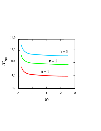
Figure 1: First mode $x_{n\nu}$ as a function
of $\omega$.

Note that the action (20) differ from dilaton action in Einstein frame in four dimensions only by the presence of n massive modes. In zero mode the mass vanishes and we use it to calculate the zero mode function $\xi_{0}$ given by Eq. (21). In this case the action is similar to the four-dimensional dilaton action. The masses given by the zeros arised from the Neumann conditions in the brane localized in $\Omega=L$. The important fact is that the brane conditions and the normalization determine the solution of the Bessel equation (24). In the Fig. 1 it is showed the dependence of the modes $x_{n\nu}$ as a function of the Brans-Dicke parameter which in next sections will be interpreted as the fine tune paramenter. We can see that this dependence presents an asymptotical behavior around $\omega=-1$.

III Charged Cosmic String Configuration in the Brane-World Scenario

In this section we study how this framework affect the cosmic string configuration in the brane. By analogy with the four dimensional Brans-Dicke theory we consider similar dilaton coupling in Einstein frame. In this case the action corresponding to a cosmic string can be written as

$${\cal S}_{CS}=\int d^{4}x\sqrt{\bar{g}}\,\,{\cal L}(\bar{g}_{\mu\nu},\phi,H_{\mu}),$$ (28)

where

$$\bar{g}_{\mu\nu} = e^{2\alpha\Phi(x,\Omega=L)}g_{\mu\nu}$$

$$\Phi(x,\Omega=L) = {1\over\sqrt{L}}\sum_{n}X_{n}(x)\,\xi_{n}(\Omega=L).$$

Now, let us investigate the cosmic string model assuming that the spacetime is approximately flat. Thus, the cosmic string action on the brane that presents a coupling with the dilaton modes at $\Omega=L$ can be written as

$$\mathcal{S}_{mat} = \Pi_{\!\!\!\!{}_{{}_{n}}}\int d^{4}x\Big{[}-\frac{1}{2}e^{2\alpha\xi_{n}X_{n}}D_{\mu}\phi(D^{\mu}\phi)^{*}$$ (29)

$$-\frac{1}{4}H_{\mu\alpha}H^{\mu\alpha}-e^{4\alpha\xi_{n}X_{n}}V(\phi)\Big{]},$$

where $\xi_{n}$ at $(\Omega=L)$ is given by equation (24).

The action given above has a $U(1)$ symmetry, associated with the $\phi$-field, which is broken by the vacuum and gives rise to vortices of the Nielsen-Olesen type Nielsen

$$\begin{array}[]{ll}\phi=\varphi(r)e^{i\theta-kL},&\\ H_{\mu}=\frac{1}{q}[P(r)-1]\delta^{\theta}_{\mu},&\end{array}$$ (30)

in which $(t,r,\theta,z)$ are usual cylindrical coordinates. The boundary conditions for the fields $\varphi(r)$ and $P(r)$ are the same as those of ordinary cosmic stringsNielsen , namely,

$$\begin{array}[]{ll}\begin{array}[]{ll}\phi(r)=\eta e^{i\theta-kL}&r\rightarrow\infty\\ \phi(r)=0&r=0\end{array}&\begin{array}[]{ll}P(r)=0&r\rightarrow\infty\\ P(r)=1&r=0,\end{array}\end{array}$$ (31)

where $D_{\mu}\phi=(\partial_{\mu}+iqH_{\mu})\phi$ is the covariant derivative. The potential $V(\phi)$ triggering the spontaneous symmetry breaking can be fixed by

$$V(\phi)=\frac{\lambda_{\phi}}{4}(|\phi|^{2}-\tilde{\eta}^{2})^{2},$$ (32)

where $\tilde{\eta}=\eta e^{-kL}$ and $\lambda_{\phi}$ is the coupling constant. Constructed in this way, this potential possesses all the ingredients that makes it to induce the formation of an ordinary cosmic string.

Let us consider that the dilaton field, propagating in the bulk is given by Maxwell-Chern-Simons three-tensor on the brane. After the integration in $\Omega$-coordinate, we have

$$\mathcal{S}_{free} \!\!= -{\frac{1}{4}}\int d^{4}x\sqrt{-{\ g}}F_{\mu\nu}F^{\mu\nu}$$ (33)

$$\mathcal{S}_{int} \!\!= \int d^{4}x\sqrt{-{\ g}}\Big{[}\sqrt{(\nu+1)kL}\,e^{-(\nu-1)kL}\partial_{\mu}X_{0}$$ (34)

$$\!\!\!\!\!\!\!\!\!\!\!\!\!\!\!\!\!\!\!\!\!\!+\,e^{\nu kL}\!\!\sum_{n=1}\!{\frac{J_{\nu}(x_{n\nu})}{N_{n}}}\!\partial_{\mu}X_{n}\!\Big{]}\Big{[}\alpha_{{}_{+}}^{{}^{\!\!(1)}}\!H_{\nu}\tilde{H}^{\mu\nu}\!\!+\!\alpha_{{}_{+}}^{{}^{\!(2)}}\!\!A_{\nu}\tilde{H}^{\mu\nu}\Big{]}$$

where $H_{\mu\nu}$ is a field strength associated with a gauge field and $\alpha_{{}_{+}}^{{}^{\!(1)}}$, $\alpha_{{}_{+}}^{{}^{\!(2)}}$ are constant coefficients.

The action (34) is the general form of the interaction terms, and is dictated by the effects that we want to analyse. The consequences of the action (34) to the cosmic string configuration can be analyzed by the equation of the motion of the gauge fields. If we consider the Ansatz for the gauge field $A_{\mu}(r)$ and the equation of motion for the gauge field $H_{\mu}(r)$ in weak field approximation, we have that the equation of the motion in Minkowiski space is

$$\partial_{\mu}H^{\mu\nu}+\epsilon^{\nu\alpha\beta\mu}\sum_{n}\xi_{n}\Big{[}\alpha_{+}^{(1)}H_{\alpha\beta}+\alpha_{+}^{(2)}F_{\alpha\beta}\Big{]}\partial_{\mu}X_{n}=J^{\nu},$$ (35)

where $j_{\mu}(\rho/\epsilon_{0},\mu J_{z})$ is given by

$$J_{\mu}={\frac{-iq}{2}}\Big{[}\phi^{*}D_{\mu}\phi-\phi(D_{\mu}\phi)^{*}\Big{]}.$$ (36)

Note that if the charge $J^{0}$ is different from zero, then $H_{t}\neq 0$. The Ansatz compatible with this configuration is

$$H_{t}(r)=0 r\rightarrow\infty$$

$$H_{t}(r)=b r=0$$ (37)

The charge behavior can be analyzed in the weak field approximation of the dilaton field as

$$A(\Phi)=A(\Phi_{(0)})+A{\acute{}}(\Phi_{(0)})\Phi_{(1)}.$$ (38)

Considering the equation of motion for the external field $F_{\mu\nu}$, we have

$$\partial_{\lambda}F^{\lambda\nu}-\alpha_{+}^{(2)}\epsilon^{\mu\nu\alpha\beta}\sum_{n}\xi_{n}\partial_{\mu}X_{n}H_{\alpha\beta}=0$$ (39)

Consider the electric field $E^{i}$ and magnetic field $B^{i}$, defined as $E^{i}=F^{0i}$ and $B^{i}=-\epsilon^{ijk}F_{jk}$. Then, we obtain

$$E_{ext} = {\frac{1}{2\pi\epsilon r}}\Big{[}\sqrt{(\nu+1)kL}\,e^{-(\nu-1)kL}\int_{0}^{r_{0}}\partial_{z}X_{0}B(r)rdr$$ (40)

$$e^{\nu kL}\sum_{n=1}{\frac{J_{\nu}(x_{n}\nu)}{N_{n}}}\int_{0}^{r_{0}}\partial_{z}X_{n}B(r)rdr\Big{]}$$

where $\varepsilon=1/\alpha_{+}^{(2)}$ This result show up that the external field generated by the charged cosmic string in this framework depends of the brane world parameters.

The energy-momentum tensor $T_{\mu\nu}$ is given by

$$T^{t}_{t} = -{\frac{1}{2}}A^{2}\Big{[}\varphi^{\prime 2}+{\frac{1}{r^{2}}}\varphi^{2}P^{2}+A^{-2}\left({\frac{A_{t}^{\prime 2}}{4\pi e^{2}}}\right)$$ (41)

$$+ \varphi^{2}H_{t}^{2}+A^{-2}{\frac{1}{r^{2}}}\left({\frac{P^{\prime 2}}{4\pi q^{2}}}\right)+2A^{2}V(\varphi)$$

$$+ A^{-2}\left({\frac{H_{t}^{\prime 2}}{4\pi e^{2}}}\right)\Big{]}$$

$$T^{z}_{z} = -{\frac{1}{2}}A^{2}\Big{[}\varphi^{\prime 2}+{\frac{1}{r^{2}}}\varphi^{2}P^{2}-A^{-2}\left({\frac{A_{t}^{\prime 2}}{4\pi e^{2}}}\right)$$ (42)

$$- \varphi^{2}H_{t}^{2}+A^{-2}{\frac{1}{r^{2}}}\left({\frac{P^{\prime 2}}{4\pi q^{2}}}\right)+2A^{2}V(\varphi)$$

$$- A^{-2}\left({\frac{H_{t}^{\prime 2}}{4\pi e^{2}}}\right)\Big{]}$$

$$T^{r}_{r} = {\frac{1}{2}}A^{2}\Big{[}\varphi^{\prime 2}-{\frac{1}{r^{2}}}\varphi^{2}P^{2}-A^{-2}\left({\frac{A_{t}^{\prime 2}}{4\pi e^{2}}}\right)$$ (43)

$$+ \varphi^{2}H_{t}^{2}+A^{-2}{\frac{1}{r^{2}}}\left({\frac{P^{\prime 2}}{4\pi q^{2}}}\right)-2A^{2}V(\varphi)$$

$$- A^{-2}\left({\frac{H_{t}^{\prime 2}}{4\pi e^{2}}}\right)\Big{]}$$

$$T^{\theta}_{\theta} = -{\frac{1}{2}}A^{2}\Big{[}\varphi^{\prime 2}-{\frac{1}{r^{2}}}\varphi^{2}P^{2}-A^{-2}\left({\frac{A_{t}^{\prime 2}}{4\pi e^{2}}}\right)$$ (44)

$$+ \varphi^{2}H_{t}^{2}-A^{-2}{\frac{1}{r^{2}}}\left({\frac{P^{\prime 2}}{4\pi q^{2}}}\right)+2A^{2}V(\varphi)$$

$$- A^{-2}\left({\frac{H_{t}^{\prime 2}}{4\pi e^{2}}}\right)\Big{]}$$

In this analysis we consider the weak field approximation, which permits us to expand the dilaton field as

$$X_{n}=X_{(0)n}+\epsilon X_{(1)n}$$ (45)

where $X_{0}$ is the constant dilaton value in the background without cosmic string.

In our framework we find the equation for the field $X_{n}$, which reads as

$$\Box X_{n} = -{\frac{1}{4}}{\frac{dU(X_{n})}{dX_{n}}}-4\pi G_{eff}C^{-1}\xi_{n}\Big{[}\alpha T$$ (46)

$$+ 2\Big{(}\alpha_{+}^{(1)}H_{\mu\nu}+\alpha_{+}^{(2)}F_{\mu\nu}\Big{)}\tilde{H}^{\mu\nu}\Big{]},$$

where the coefficients $\alpha_{{}_{+}}^{{}^{\!(1)}}$ and $\alpha_{{}_{+}}^{{}^{\!(2)}}$ are associated with the topological contributions. The terms whose coefficients are $\alpha_{{}_{+}}^{{}^{\!(1)}}$ and $\alpha_{{}_{+}}^{{}^{\!(2)}}$ vanishe because the fields does not depend on $t$ and $z$. Thus, we obtain

$$\Box X_{n}=-{\frac{1}{4}}{\frac{dU(X_{n})}{dX_{n}}}-4\pi G_{eff}C^{-1}\xi_{n}\alpha T$$ (47)

Let us consider the solution as

$$X_{n}(t,r,z)=\chi_{n}(r)+f(r)\Xi_{n}(t,z)$$ (48)

where $f(r)$ is required to vanishes outside the string core. The charge induced by the dilaton is

$$Q\! \!=\! \!2\pi\alpha_{+}^{{}^{\!(1})}\!\Big{[}\!\alpha\sqrt{(\nu\!+\!1)kL}\,e^{-(\nu-1)kL}\partial_{z}\Xi_{0}\int_{0}^{r_{0}}\!\!\!\!f(r)B(r)rdr$$ (49)

$$\,e^{\nu kL}\!\!\sum_{n=1}{\frac{J_{\nu}(x_{n\nu})}{N_{n}}}\partial_{z}\Xi_{n}\int_{0}^{r_{0}}f(r)B(r)rdr\Big{]}$$

Using solution (48), we obtain to first order in $G_{eff}$, the equation

$$\chi_{n}^{\prime\prime}+{\frac{1}{r}}\chi_{n}^{\prime}+m_{n}^{2}\chi_{n}=-\,4\pi\,G_{eff}\,\xi_{n}\,C^{-1}\alpha\,\tilde{T}_{(0)}$$

The field $\Xi$, obeys the following equations

$${\frac{\partial^{2}f}{\partial r^{2}}}+{\frac{1}{r}}{\frac{\partial f}{\partial r}} = \omega_{n}^{2}f$$ (50)

$${\frac{\partial^{2}\Xi_{n}}{\partial t^{2}}}-{\frac{\partial^{2}\Xi_{n}}{\partial z^{2}}} = \omega_{n}^{2}\Xi_{n}$$ (51)

where $f$ satisfies the boundary condition at $r\rightarrow\infty$. The arbitrary constant $w_{n}$ can assume, a priori, both positive and negative values for each n as $\omega^{2}=k^{2}-\omega_{0}^{2}$. The solution of the equations of motion (50) and (51) are important to discuss the aspects connected with the change the charge. Considering the well known electric case, let us take $w=k$. Thus, the solution for $f$ is

$$f(r)=f_{I}I_{0}(kr)+f_{k}K_{0}(kr)$$ (52)

where $I_{0}$ and $K_{0}$ are modified Bessel functions of order zero. The function $I_{0}$ is exponentially divergent for large values of the argument, then we choose $f_{I}=0$ in order to have $f(r)=0$ when $r\rightarrow\infty$. Thus, $\Xi$ has an oscillatory solution and can be written as

$$\Xi_{n}(z) = \Xi_{(0)n}\cos{k_{n}z}$$ (53)

The energy momentum tensor that is relevant in the weak field approximation is $T_{(0)\,\mu\nu}$, which in this charged model is given by

$$T_{tt} = U\delta(x)\delta(y)+{\frac{Q}{4\pi}}\nabla^{2}\Big{(}\ln{\frac{r}{r_{0}}}\Big{)}\noindent$$ (54)

$$T_{zz} = -\tau\delta(x)\delta(y)+{\frac{Q}{4\pi}}\nabla^{2}\Big{(}\ln{\frac{r}{r_{0}}}\Big{)}$$ (55)

$$T_{(ij} = -Q^{2}\delta_{ij}\delta(x)\delta(y)+{\frac{Q}{2\pi}}\partial_{i}\partial_{j}\Big{(}\ln{\frac{r}{r_{0}}}\Big{)}$$ (56)

where, $U$ and $\tau$ are the energy per unit length and the tension per unit length, respectively. The other result associated with the Brane-World parameters is the polarization of the radiation coming from cosmological distant sources.

The mass $m_{n}$ is small compared with as oscillation frequency of the loop. The relevant part of the dilatonic contribution is the $\chi_{n}$ solution which in our model is given by

$$\chi_{0} \!\!\!= \!\!\!\!2G_{{}_{\!\!eff}}C^{{}^{-1}}\!\!\!\!\!\alpha\sqrt{(\nu\!+\!1)kL}\,e^{-(\nu-1)kL}\Big{(}\!U\!+\!\tau+\!{\frac{Q^{2}}{\varepsilon^{2}}}\!\Big{)}\ln(\!{\frac{r}{r_{0}}}\!)$$

$$\chi_{n} \!\!= \!\!\!2G_{{}_{\!eff}}\!C^{{}^{-1}}\!\!\!\!\alpha\,\,e^{\nu kL}{\frac{J_{\nu}(x_{n\nu})}{N_{n}}}\Big{(}\!U\!+\!\tau\!+\!{\frac{Q^{2}}{\varepsilon^{2}}}\Big{)}\ln({\frac{r}{r_{0}}})$$ (57)

This result is different from the usual case Bezerra:2004qv because in this framework there are ”n” scalar fields corresponding to the oscillation-modes and each frequency is related with one energy scale.

IV Cosmic Microwave Background Radiation and cosmic optical activity

In this section, we consider the Brans-Dicke parameter and the possibility to obtain a model to understand the cosmic optical activity. Some authors analyzed the possibility that optical polarization of light from quasars and galaxies can provide evidence for cosmical anisotropy Hutsemekers . The idea is that in some conditions the spacetime can exhibit different properties such as the optical activity or birefringence [Das ; Nodland97a ; Nodland97b . It is well known that, as a consequence of vacuum polarization effects in QED Heisenberg ; Weisskopf ; Dittrich ; Schwinger , the electromagnetic vacuum presents a birefringent behavior Klein ; Adler ; Brezin ; Bialynicka . For example, in the presence of an intense static background magnetic field, there are two different refraction indices depending on the polarization of the incident electromagnetic wave. This is in fact a very tiny effect which could be measured in a near future Heinzl . The present bounds for this anisotropy, followed from several experimentsSemertzidis ; Cameron ; Zavattini ; Zavattini2 , are still far from the expected value from QED. For this study let us consider the cosmic string background in the context of the perturbed scalar compactification from 5-dimensions given by scalar-tensor theory Brane-World scenario, which can be written as

$$\mathcal{S}_{int} \!\ \!\!\!\!=\!\!\! \!\int\!\!\!d^{4}x\sqrt{\!\!-{\!g}}\Big{(}-\!\!\!\!\!{\!\!\frac{1}{4}}F_{\mu\nu}F^{\mu\nu}\!\!+\!\alpha_{+}^{{}^{\!\!(3)}}\!\!\sum_{n}\!\!\xi_{n}\partial_{\mu}X_{n}A_{\nu}\tilde{F}^{\mu\nu}\!\Big{)}$$ (58)

in which we couple the electromagnetic field strenght $F_{\mu\nu}$ and the vector potential $A_{\nu}$ with the n modes of the dilaton. In this context the equation of the motion for the electromagnetic field becomes

$$\partial_{\mu}F^{\mu\nu}=2\alpha_{+}^{(3)}\sum_{n}\xi_{n}\partial_{\mu}X_{n}\tilde{F}^{\mu\nu}$$ (59)

The solutions of the Eq.(59) give us the corresponding dispersion relation

$$(k^{\alpha}k_{\alpha})^{2}+(k^{\alpha})k_{\alpha}(v^{\beta}v_{\beta})=(k^{\alpha}v_{\alpha})^{2}$$ (60)

where $v_{\mu\,n}=\partial_{\mu}X_{n}$ is responsible for the appearance of the prefered cosmic direction, as suggested by the observations Hutsemekers . We can expand the dispersion relation given by Eq.(60)in powers of $v_{\alpha}$. In this case we find the dispersion relation in power of $\phi_{\alpha}$, considering the linearized solution in $\phi$ to the first order, giving us

$$k_{n\,\pm}\!=\!\omega_{n}\pm 2\alpha_{+}^{(3)}\alpha_{n}C^{{}^{\!-1}}\!\xi^{2}_{n}G_{{}_{\!eff}}\mu\,\,{\hat{s}}\cos(\gamma)$$ (61)

with $\mu=(U+\tau+\Big{(}{\frac{Q}{\epsilon}}\Big{)}^{2})$, $\omega$ and $k$ being the wave frequency and wave vector, respectively, the 4-vector $k^{\alpha}=(\omega,k);k=|k|$ and $\gamma$ the angle between the propagation wavevector k of the radiation and the unit vector ${\hat{s}}$.

Let us contextualize our theoretical results in the framework of the conclusions drawn from the analysis of observational data from quasar emission performed by Nodland97a ; Jain ; Das . The angle $\gamma$ between the polarization vector and the galaxies major axis is defined as $<\beta_{n}>={\frac{r}{2}}\Lambda_{n}\cos(\vec{k},\vec{s})$, where $<\beta_{n}>$ represents the mean rotation angle after Faraday rotation is removed, r is the distance to the galaxy, $\vec{k}$  the wavevector of the radiation, and $\vec{s}$ a unit vector defined by the direction on the sky. The Lorentz breaking imposes that the prefered vector is in $r$ direction. The rotation of the polarization plane is a consequence of the difference between the propagation velocity of the two modes $k_{+},k_{-}$, the main dynamical quantities. This difference, defined as the angular gradient with respect to the radial (coordinate) distance, is expressed as ${\frac{1}{2}}(k_{+}-k_{-})={\frac{d\beta_{n}}{dr}}$, where $\beta_{n}$ measures the specific entire rotation of the polarization plane, per unit length r, and is given by $\beta_{n}={\frac{1}{2}}\Lambda_{n}^{-1}r\,\cos\,\gamma$. In the case of the cosmic string solution in compactified scalar brane world scenarios we have

$$\Lambda_{n}^{-1}=2\alpha_{+}^{(3)}C^{-1}\alpha_{n}\,\xi_{n}^{2}G_{{}_{\!eff}}\,\mu$$ (62)

If we consider that this result is compatible with the Cosmic Microwave Background (CMB) radiation, up to mode $n$, we obttain

$$2\alpha_{n}C^{-1}\xi_{n}G_{{}_{\!eff}}\,\mu\sim 10^{-6}.$$ (63)

The other important aspect that we must analyse is the hierarchy problem related with the constant $\alpha_{0}$. So by compatibility with CMB radiation, constraint (63) must be satisfied. Then, for $n=0$ we have the zero mode given by

$$C^{-1}\alpha_{0}\sim 0,5[12(\nu+1)]^{-1/2}\,e^{-12(\nu-1)}$$ (64)

where $G_{{}_{eff}}\,\mu\sim 10^{-6}$ because $G_{{}_{eff}}\sim 10^{-38}$ and the energy density per unit of lenght $\mu$ of the cosmic string is equal to the symmetry breaking scale $\eta^{2}$, where $\eta$ is of the order of $10^{16}$.

Let us analyse the numerical constraints imposed by CMB radiation and the Brans-Dicke parameter $\omega$ taking into account the compactification modes. In this scenario we use the value of $\Lambda^{-1}$ limit of the order of $10^{-32}$ eV Nodland97a .

In order to analyse the contribution of the Lorentz breaking term in the Universe we must understand how the parameters of our model are related with the physical effects. The parameter that is importat here is the dependence of the coupling constant $\Lambda^{-1}$ with the Brans-Dicke parameter $\omega$ to each modes. This dependence must be a constraint in the range of validity of the coupling constant $\Lambda^{-1}$.

In this framework the zero mode is responsible by an important number of phenomenological implications Giudice99 ; Cullen99 and is only coupled with gravitational fields and, in our approach, with the electromagnetic field strength. The dependence of the zero mode coupling constant $\Lambda_{0}^{-1}$ with the Brans-Dicke parameter $\omega$ is given by

$${\Lambda}_{0}^{-1}=10^{-40}[(\nu+1)\,kL]^{1/2}\,e^{(\nu-1)kL},$$ (65)

where we choose the parameter $\alpha_{+}=10^{-34}$ . We can see from Fig.2 that the expression of $\nu$ as function of $\omega$ is dimension dependent and the expression is given by $\nu={(D-1)w+D\over 2(w+1)}$ Bayona:2008ui . In our case D=5 and the expression reduces to $\nu={(4w+5)\over(2w+2)}$ .

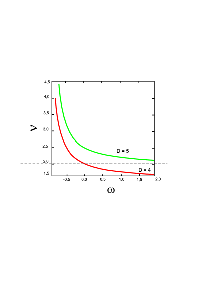
Figure 2:  Dependence of the parameter $\nu$ as a function of $\omega$ corresponding to D=4 and D=5.

Note in Fig. 2 that when $\omega\rightarrow\infty$, then $\nu$ goes to 2 and gives us an assymptotical limit ${\Lambda}_{0}^{-1}=0,98\times 10^{-32}$, if we choose $kL=12$ Goldberger:1999wh . This limit corresponds to a lower bound. This model presents another limit where $\omega$ goes to $-1$ and ${\Lambda}_{0}^{-1}\rightarrow\infty$. This upper assymptotical value does not have physical application. We note that the value of $\omega$ taken into account for the fine tune in our model must be linked with experimental data. The range of values that we are considering here is showed in Fig. 3 which presents also comparison with the massive mode $n=1$.

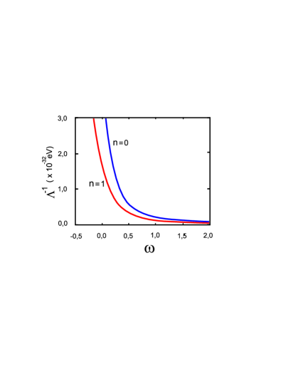
Figure 3: Parameter $\Lambda^{-1}$ for $n\neq 0$ in terms of $\omega$.

The behavior of the massive modes is given by the expression

$$\Lambda^{-1}_{1}={10^{-40}\over N_{1}}J_{\nu}(x_{1\nu}).$$ (66)

We can analyse the $n=1$ massive mode in Fig. 3. We note, by comparing with the $n=0$ case that the value of $\Lambda^{-1}$ decreases. This fact can be understood if we consider that in order to activate this mode we need more energy by the fact that this mode is massive and can be important in events that involves high energy.

V Particle production in the Brane-World Scenario

In this section we consider the dilaton production given by the oscillating loops of the cosmic string that can decay in gauge bosons.

The loop cosmic string studied in section III couples with the compactified dilaton modes at diferent energies that coincides with the loop oscillator frequencies. During this process, massive dilatons are copiously emitted with frequency of oscillation greater than the dilaton mass.

To take into account the dilaton decay in gauge bosons we need the interaction with the electromagnetic field. Therefore, we must consider another type of term where the dilaton with spin-0 particles couples with the electromagnetic field through the mass term with coupling constant, $\alpha_{-}\neq 0$.

In this section the zero mode is not considered because this mode corresponds to zero mass. The interaction action responsible for decays into gauge bosons is after the integration of the $\Omega$-component given by

$$\mathcal{S}_{int}\!\!=\alpha_{-}\!\!\!\!\sum_{n=1}e^{\nu kL}{\frac{J_{\nu}(x_{n\nu})}{N_{n}}}\int\!d^{4}x\sqrt{-{g}}X_{n}\!F_{\mu\nu}F^{\mu\nu}$$ (67)

The mass of the dilaton in our model is given by the compactification scales and the coupling is related with the mode function $\xi_{n}$.

In our model the energy spectrum and angular distribution of the dilaton radiation can be determined by generalization of the results obtained in Damour97 to include the n modes and consider a charged cosmic string.

If we have a loop with length L, $\omega_{n}=4\pi n/L$, the sums are taken over $n>L/L_{c}$, where $L_{c}=4\pi/m_{n}$. The important point of our work is that for each n we have a different mass for the dilaton given by $m_{n}=x_{n\nu}\kappa e^{-\kappa L}$, in accordance with we have aleady obtained in secton II. These masses also have dependence on $\nu$ that has constraint given by the Brans-Dicke parameter as showed in Fig. 4.

The parameters $x_{n\nu}$ can be determined as function of the Brans Dicke parameter $\omega$. The energy range that we consider as a function of $\kappa L$ are specified in Fig. 5, considering the constant $\kappa$ in Planck scale.

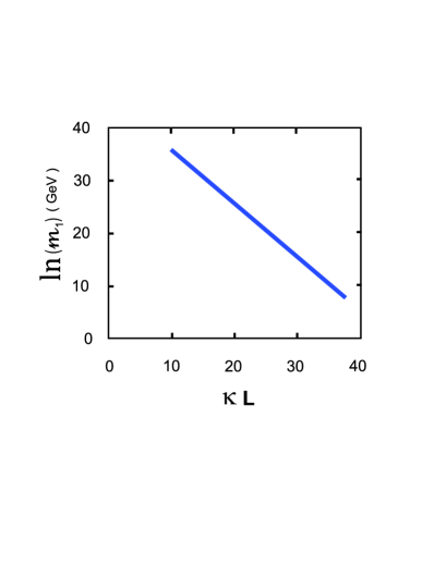
Figure 4:   Mass for n=1 as a function of $\kappa L$.

In the context of the dilaton, the energy scales are compatible with the references Ellis86 . In our model, in order to find masses with this energy of the order of TeV for $n=1$, we have $kL\sim 40$. In this process there is the possibility to generate light gauge bosons. However if we consider $\kappa L=12$, as in last section, the particles masses are of the order of $(\sim 10^{14})GeV$. These values for the masses can be mensurable in the Pierre Auger experiment, for example. The decays of these massive particles can be detected, in principle, with lower energies.

The energy and particle radiation rates when the loop is such that $L>>L_{c}$ have a mode dependence which can be represented as

$$\dot{E}_{X_{n}} = \Gamma_{X_{n}}\alpha_{n}^{2}G_{eff}U^{2}(L/L_{c})^{-1/3}$$ (68)

$$\dot{N}_{X_{n}} = \tilde{\Gamma}_{X_{n}}\alpha_{n}^{2}G_{eff}U^{2}m_{X_{n}}^{-1}(L/L_{c})^{-1/3}$$ (69)

The resulting constraints are relevant if we consider the life-time of the dilaton, that are determined by the mass and couplings. The corresponding lifetime is

$$\tau_{n}={\frac{4M_{p}^{2}}{N_{F}\tilde{\alpha}^{2}_{F_{n}}m^{3}_{n}}}$$ (70)

where $\tilde{\alpha}_{F_{n}}=\alpha_{-}\alpha_{n}C^{-1}\xi_{n}$ and $N_{F}$ is the number of gauge bosons with masses $<<m_{X_{n}}$. In Fig. 5 we consider $m_{X_{n}}\sim 1$ TeV. In this case all standard-model gauge bosons should be included ($N_{F}=12$). We note that the lifetime of the dilatons has a fine structure constant given by the Brans-Dicke parameter. It is important to ajust with the experimental data. Here we also have the constraints given by the Brans-Dicke parameter $\omega$. For $\omega=-1$ the lifetime agrees at infinity, giving us the possibility that massive particles decay in the primordial Universe and probably could be measured in the detectors nowadays.

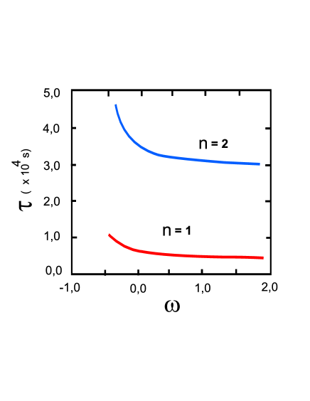
Figure 5: This graphic represent the the lifetime of the particles in function of the Brans-Dicke parameter.

VI Conclusions

It is possible to construct a Brane-World scenario including gravity in which we can analyse the effects of the Lorentz Breaking in the framework of a cosmic string configuration. With this aim we can assume that the scalar tensor theory is realized in 5-dimensions. In this scenario it is showed that the cosmological birefringence is connected with the Brans-Dicke parameter which is constrained by the date of the Cosmic Microwave Background Radiation and by the compactification modes. The limits of the rotation angle depends on the Brans-Dicke parameter and decreases with the increasing of masses of the correpsonding massive modes.

In this framework of saclar-tensor theory of gravity in 5-dimensions, the ineraction terms can be taken with and without parity violation. These terms are connected with the cosmic string configuration we are considering. The Lorentz breaking term is responsible for generation of charge and the part that does not present the parity violation put limits on the mass scale of the particles which decay into light dilaton. The interaction Lagrangian (67) is responsible for the decay into light gauge bosons, where are the sources of cosmic strings. These depend on the modes given by the 5-dimensional Brane-World scenario.

Acknowledgments: The authors would like to thank (CNPq-Brazil) for financial support. C. N. Ferreira also thank Centro Brasileiro de Pesquisas Físicas (CBPF) for hospitality. V. B. Bezerra also thanks FAPESQ-PB (PRONEX) and FAPES-ES (PRONEX). G. de A. M. tanks FAPESQ - PB (PRONEX).

References

- (1) e-mail: valdir@fisica.ufpb.br
- (2) e-mail: crisnfer@cefetcampos.br
- (3) e-mail:gmarques@df.ufcg.edu.br
- (4) A.Vilenkin, Phys. Rev. D 23, 852 , (1981); W.A.Hiscock, Phys. Rev. D 31, 3288, (1985); J.R.GottIII, Astrophys. Journal, 288, 422, (1985).
- (5) T. W. B. Kibble, Phys. Rep. 67, 183 (1980); A. Vilenkin, Phys. Rev. D 23, 852 (1981).
- (6) J. Audretsch, U. Jasper and V. D. Skarzhinsky, Phys. Rev. D 49, 6576, (1994).
- (7) T. M. Helliwell and D. A. Konkowski, Phys. Rev. D 34, 1918 (1986); V. P. Frolov and E. M. Serebriany, Phys Rev. D 35, 3779 (1987).
- (8) M. Green, J. Schwarz and E. Witten, Superstring Theory (Cambridge: Cambridge University Press) (1987).
- (9) C. Brans and R. H. Dicke, Phys. Rev. 124, 925 (1961);
- (10) L. H. Ford and T. Yoshimura, Phys. Lett. A 70, 89 (1979): D. J. Toms, Phys. Rev. D21, 928 (1980).
- (11) S. D. Odnitsov, Sov. J. Nuch. Phys. 48, 1148 (1988).
- (12) N. Arkani-Hamed, S. Dimopoulos, and G. Dvali, Phys Lett. B 429, 263 (1998); I. Antoniadis, N. Arkani-Hamed, S. Dimopoulos and G. R. Dvali, Phys. Lett. B 436 (1998) 257.
- (13) L. Randall and R. Sundrum, Phys. Rev. Lett. 83, 3370 (1999); Phys. Rev. Lett. 83, 4690 (1999).
- (14) H. B. Nielsen and P. Olesen, Nucl. Phys. B 61, 45 (1973).
- (15) V.B.Bezerra, C. N. Ferreira and J. A. Helayel-Neto, Phys. Rev. D 71, 044018 (2005)
- (16) D. Hutsemekers and H. Lamy, Astron. Astrophys. 367, 381 (2001).
- (17) P. Das, P. Jain, S. Mukherji, Int. J. Mod. Phys. A16 4011 (2001).
- (18) B. Nodland and J. P. Ralston, Phys. Rev. Lett. 78, 3043 (1997); 79, 1958 (1997).
- (19) B. Nodland and J. P. Ralston, Cosmologicaly Screwy Light, astro-ph/9704197; Proceedings of the 14th Particles and Nuclei International Conference (PANIC), (1996). Eds. C. Carlson et al, World Scientific, Singapore (1997).
- (20) W. Heisenberg and H. Euler, Z. Phys. 98, 714 (1936).
- (21) V. Weisskopf, The electrodynamics of the vacuum based on the quantum theory of electrons, English translation in Early Quantum Electrodynamics: A source book, A.I. Miller Edt. Cambridge University Press (1994).
- (22) W. Dittrich and H. Gies, Probing the Quantum Vacuum: Perturbative Effective Action Approach in Quantum Electrodynamics and Its Applications, Springer Tracts in Modern Physics 2000.
- (23) J. Schwinger, Phys. Rev. 82, 664 (1951).
- (24) J. Klein and B. Nigam, Phys. Rev. 135, 1279 (1964).
- (25) S. L. Adler, Ann. Phys. (N.Y.) 67, 599 (1971).
- (26) E. Brezin and C. Itzykson, Phys. Rev. D3, 618 (1971).
- (27) Z. Bialynicka-Birula and I. Bialynicka-Birula, Phys. Rev. D2, 2341 (1970).
- (28) T. Heinzl, B. Liesfeld, K. Amthor, H. Schwoerer, R. Sauerbrey and A. Wipf, Optics Communications 267, 318 (2006).
- (29) Y. Semertzidis et al. [BFRT Collaboration], Phys. Rev. Lett. 64, 2988 (1990).
- (30) R. Cameron et al [BFRT Collaboration], Phys. Rev. D47, 3707 (1993).
- (31) E. Zavattini et al. [PVLAS collaboration], Phys. Rev. Lett. 96, 110406 (2006).
- (32) E. Zavattini, et al. [ PVLAS collaboration], Phys. Rev. D 77, 032006 (2008).
- (33) P. Jain, J. P. Ralston, Mod. Phys. Lett. A14, 417 (1999).
- (34) G. F. Giudice, R. Ratazzi and J. D. Wells, Nucl. Phys. B544, 3 (1999): E. A. Mirabelli, M. Perelstein and M. E. Peskin, Phys. Rev. Lett. 82, 2236 (1999); T. Han, J. D. Lykken and R. J. Zhang, Phys. Rev D 59, 105006; JoAnne L. Hewett, Phys. Rev Lett. 82,4765 (1999).
- (35) S. Cullen and M. Perelstein, SN1987A (Ver Publcacao)
- (36) C. A. B. Bayona and C. N. Ferreira, D-dimensional Randall Sundrum models from Brans Dicke Theory and Kaluza-Klein modes, arXiv:08121621.
- (37) W. D. Goldberger and M. B. Wise, Phys. Rev. D 60, 107505 (1999).
- (38) T. Damour and A. Vilenkin, Phys. Rev. Lett. 78, 2288. (1997).
- (39) J. Ellis, D.V. Nanopoulos and M. Quiros, Phys. Lett. B174, 176 (1986); J. Ellis, N.C. Tsamis and M. Voloshin, Phys. Lett. B194, 291 (1987)