Gradient Estimates for the Subelliptic Heat Kernel on H-type Groups

Abstract

We prove the following gradient inequality for the subelliptic heat kernel on nilpotent Lie groups $G$ of H-type:

$$\left|\nabla P_{t}f\right|\leq KP_{t}(\left|\nabla f\right|)$$

where $P_{t}$ is the heat semigroup corresponding to the sublaplacian on $G$, $\nabla$ is the subelliptic gradient, and $K$ is a constant. This extends a result of H.-Q. Li [10] for the Heisenberg group. The proof is based on pointwise heat kernel estimates, and follows an approach used by Bakry, Baudoin, Bonnefont, and Chafaï [3].

url]http://www.math.cornell.edu/ neldredge/

1 Introduction

In [10], H.-Q. Li proved the following gradient inequality for the heat kernel on the classical Heisenberg group $\mathbb{H}_{1}$ of real dimension $3$:

$$\left|\nabla P_{t}f\right|\leq KP_{t}(\left|\nabla f\right|)$$ (1.1)

where $P_{t}$ is the heat semigroup corresponding to the usual sublaplacian on $\mathbb{H}_{1}$, $\nabla$ is the corresponding subgradient, $K$ is a constant, and $f$ is any appropriate smooth function on $\mathbb{H}_{1}$. This was the first extension of (1.1) to a subelliptic setting; the elliptic case was shown by Bakry [1], [2], and in the case of a Riemannian manifold corresponds to a lower bound on the Ricci curvature.

The proof in [10] relies on pointwise upper and lower estimates for the heat kernel, and a pointwise upper estimate for its gradient, both of which were obtained in [11] in the context of Heisenberg groups of any dimension. [3] contains two alternate proofs of (1.1) for the classical Heisenberg group $\mathbb{H}_{1}$, also depending on the pointwise heat kernel estimates from [11]. Earlier, Driver and Melcher in [5] had shown a partial result: that for any $p>1$ there exists a constant $K_{p}$ such that

$$\left|\nabla P_{t}f\right|^{p}\leq K_{p}P_{t}(\left|\nabla f\right|^{p}).$$ (1.2)

Their argument proceeded probabilistically via methods of Malliavin calculus and did not depend on heat kernel estimates, but they also showed that it could not produce (1.1), which is the corresponding estimate with $p=1$. [13] extended the “$L^{p}$-type” inequality (1.2) to the case of a general nilpotent Lie group, at the cost of replacing the constant $K_{p}$ with a function $K_{p}(t)$.

In [6], we were able to show that pointwise heat kernel estimates analogous to those of [11] (see (2.8–2.10)) hold for Lie groups of H type, a class which generalizes the Heisenberg groups while retaining some rather strong algebraic properties. (H-type groups were introduced by Kaplan in [9]; a useful reference and primer is Chapter 18 of [4].) The purpose of the present article is to show that given these heat kernel estimates, the first proof from [3] can be adapted to establish the inequality (1.1) in the setting of H-type groups. Our proof approximately follows the structure of the first proof from [3] but may be read independently of it, and is more explicitly detailed.

2 Definitions and notation

In order to fix notation, we give a definition of H-type groups and accompanying concepts. Our notation, where applicable, matches that of [6].

A finite-dimensional Lie algebra $\mathfrak{g}$ (with nonzero center $\mathfrak{z}$), together with an inner product $\left\langle\cdot,\cdot\right\rangle$, is said to be of H type or Heisenberg type if the following conditions hold:

1. $[\mathfrak{z}^{\perp},\mathfrak{z}^{\perp}]=\mathfrak{z}$; and

2. For each $z\in\mathfrak{z}$, the map $J_{z}:\mathfrak{z}^{\perp}\to\mathfrak{z}^{\perp}$ defined by

   $$\left\langle J_{z}x,y\right\rangle=\left\langle z,[x,y]\right\rangle\quad\text{for $x,y\in\mathfrak{z}^{\perp}$}$$ (2.1)

   is an orthogonal map when $\left\langle z,z\right\rangle=1$.

A connected, simply connected Lie group $G$ is said to be of H type if its Lie algebra $\mathfrak{g}$ is equipped with an inner product satisfying the above conditions.

It is easy to see that an H-type Lie algebra (respectively, Lie group) is a step 2 stratified nilpotent Lie algebra (Lie group). The special case $m=1$ produces the isotropic Heisenberg or Heisenberg-Weyl groups, and the case $n=m=1$ gives the classical Heisenberg group $\mathbb{H}_{1}$ of dimension $3$ discussed in [3].

As usual, $G$ can be identified as a set with $\mathfrak{g}$, taking the exponential map to be the identity. By fixing an orthonormal basis for $\mathfrak{g}=\mathfrak{z}^{\perp}\oplus\mathfrak{z}$, we can identify $G$ and $\mathfrak{g}$ with Euclidean space equipped with an appropriate bracket, as the following proposition states. (The proof is uncomplicated.)

Proposition 2.1.

If $G$ is an H-type Lie group identified with its Lie algebra $\mathfrak{g}$, then there exist integers $n,m>0$, a bracket operation $[\cdot,\cdot]$ on $\mathbb{R}^{2n+m}=\mathbb{R}^{2n}\times\mathbb{R}^{m}$, and a map $T:G\to\mathbb{R}^{2n+m}$ such that $T:\mathfrak{g}\to(\mathbb{R}^{2n+m},[\cdot,\cdot])$ is a Lie algebra isomorphism, $T\mathfrak{z}=0\times\mathbb{R}^{m}$, and $T$ is an isometry with respect to the inner product $\left\langle\cdot,\cdot\right\rangle$ on $\mathfrak{g}$ and the usual Euclidean inner product on $\mathbb{R}^{2n+m}$. If we define a group operation $\star$ on $\mathbb{R}^{2n+m}$ as usual via $v\star w=v+w+\frac{1}{2}[v,w]$, then $T:G\to(\mathbb{R}^{2n+m},\star)$ is a Lie group isomorphism, which maps the center of $G$ to $0\times\mathbb{R}^{m}$. The identity of $G$ is $0$ and the group inverse is given by $g^{-1}=-g$.

Henceforth we make this identification, and assume that our Lie group $G$ is just $\mathbb{R}^{2n+m}$ with an appropriate bracket $[\cdot,\cdot]$ and corresponding group operation $\star$. We let $\{e_{1},\dots,e_{2n}\}$ denote the standard orthonormal basis for $\mathbb{R}^{2n}\times 0\subset G$, and $\{u_{1},\dots,u_{m}\}$ the standard orthonormal basis for $0\times\mathbb{R}^{m}\subset G$, and write elements of $G$ as $g=(x,z)=\sum_{i}x^{i}e_{i}+\sum_{j}z^{j}u_{j}$. The maps $J_{z}$ can then be identified with skew-symmetric $2n\times 2n$ matrices, which are orthogonal when $\left|z\right|=1$.

We remark a few obvious consequences of (2.1):

Proposition 2.2.

1. $J_{z}$ depends linearly on $z$;

2. $\left|J_{z}x\right|=\left|z\right|\left|x\right|$, and by polarization $\left\langle J_{z}x,J_{w}x\right\rangle=\left\langle z,w\right\rangle\left|x\right|^{2}$ and $\left\langle J_{z}x,J_{z}y\right\rangle=\left|z\right|^{2}\left\langle x,y\right\rangle$;

3. $\left\langle J_{z}x,x\right\rangle=0$, so $J_{z}^{*}=-J_{z}$.

4. $J_{z}^{2}=-\left|z\right|^{2}I$.

We note that Lebesgue measure $m$ on $\mathbb{R}^{2n+m}=G$ is bi-invariant under the group operation, and thus $m$ can be taken as the Haar measure on the locally compact group $G$.

For $i=1,\dots,2n$, let $X_{i}$ be the unique left-invariant vector field on $G$, and $\hat{X}_{i}$ the unique right-invariant vector field, such that $X_{i}(0)=\hat{X}_{i}(0)=\frac{\partial}{\partial x^{i}}$. We can write

$$X_{i}f(g)=\left.\frac{d}{ds}\right|_{s=0}f(g\star(se_{i},0)),\quad\hat{X}_{i}f(g)=\left.\frac{d}{ds}\right|_{s=0}f((se_{i},0)\star g).$$ (2.2)

A straightforward calculation shows

$$\begin{split}X_{i}&=\frac{\partial}{\partial x^{i}}+\frac{1}{2}\sum_{j=1}^{m}\left\langle J_{u_{j}}x,e_{i}\right\rangle\frac{\partial}{\partial z^{j}}\\ \hat{X}_{i}&=\frac{\partial}{\partial x^{i}}-\frac{1}{2}\sum_{j=1}^{m}\left\langle J_{u_{j}}x,e_{i}\right\rangle\frac{\partial}{\partial z^{j}}\end{split}$$ (2.3)

We note that $[X_{i},\hat{X}_{j}]=0$ for all $i,j$.

As a consequence of the H-type property, the collection $\{X_{i}(g),[X_{i},X_{j}](g):i,j=1,\dots,2n\}\subset T_{g}G$ spans $T_{g}G$ for each $g\in G$. Such a collection is said to be bracket-generating.

The left-invariant subgradient $\nabla$ on $G$ is given by $\nabla f=(X_{1}f,\dots,X_{2n}f)$, with the right-invariant $\hat{\nabla}$ defined analogously. We shall also use the notation $\nabla_{x}f:=\left(\frac{\partial}{\partial x^{1}}f,\dots,\frac{\partial}{\partial x^{2n}}f\right)$ and $\nabla_{z}f:=\left(\frac{\partial}{\partial z^{1}}f,\dots,\frac{\partial}{\partial z^{m}}f\right)$ to denote the usual Euclidean gradients in the $x$ and $z$ variables, respectively. Note that $\nabla_{z}$ is both left- and right-invariant. From (2.3) it is easy to verify that

$$\begin{split}\nabla f(x,z)&=\nabla_{x}f(x,z)+\frac{1}{2}J_{\nabla_{z}f(x,z)}x\\ \hat{\nabla}f(x,z)&=\nabla_{x}f(x,z)-\frac{1}{2}J_{\nabla_{z}f(x,z)}x\end{split}$$ (2.4)

In particular, since $J_{z}$ depends linearly on $z$ and is orthogonal for $\left|z\right|=1$, we have

$$\left|(\nabla-\hat{\nabla})f(x,z)\right|=\left|x\right|\left|\nabla_{z}f(x,z)\right|.$$ (2.5)

We shall make use of this fact later.

The left-invariant sublaplacian $L$ is the second-order differential operator defined by $L=X_{1}^{2}+\dots+X_{2n}^{2}$; $L$ is subelliptic but not elliptic. By a renowned theorem due to Hörmander [7], the bracket-generating condition implies that $L$ is hypoelliptic, so that if $Lf\in C^{\infty}$ then $f\in C^{\infty}$; the same holds for the heat operator $L-\frac{\partial}{\partial t}$. $L$ is an essentially self-adjoint operator on $L^{2}(m)$, and we let $P_{t}:=e^{tL}$ be the heat semigroup corresponding to $L$. $P_{t}$ has a convolution kernel $p_{t}$, so that

$$P_{t}f(g)=\int_{G}f(g\star k)p_{t}(k)\,dm(k).$$ (2.6)

By hypoellipticity, $p_{t}$ is a smooth function on $G$. An explicit formula for $p_{t}$ is known:

$$p_{t}(x,z)=(2\pi)^{-m}(4\pi)^{-n}\int_{\mathbb{R}^{m}}e^{i\left\langle\lambda,z\right\rangle-\frac{1}{4}\left|\lambda\right|\coth(t\left|\lambda\right|)\left|x\right|^{2}}\left(\frac{\left|\lambda\right|}{\sinh(t\left|\lambda\right|)}\right)^{n}\,d\lambda.$$ (2.7)

See, among others, [15] for a derivation of (2.7). We note in particular that $p_{t}$ is a radial function; i.e. $p_{t}(x,z)$ is a function of $\left|x\right|,\left|z\right|$. This is unsurprising in light of the fact, easily verified, that $L$ maps radial functions to radial functions.

For $\alpha>0$, define the dilation $\varphi_{\alpha}:G\to G$ by $\varphi_{\alpha}(x,z)=(\alpha x,\alpha^{2}z)$; then $\varphi_{\alpha}$ is a group automorphism of $G$. A straightforward computation shows that $X_{i}(f\circ\varphi_{\alpha})=\alpha(X_{i}f)\circ\varphi_{\alpha}$, and $P_{t}(f\circ\varphi_{\alpha})=(P_{\alpha^{2}t}f)\circ\varphi_{\alpha}$.

We now make some definitions concerning the geometry of $G$. An absolutely continuous path $\gamma:[0,1]\to G$ is said to be horizontal if there exist absolutely continuous $a_{i}:[0,1]\to\mathbb{R}$ such that $\dot{\gamma}(t)=\sum_{i=1}^{2n}a_{i}(t)X_{i}(\gamma(t))$. In such a case the speed of $\gamma$ is given by $\lVert\dot{\gamma}(t)\rVert:=\left(\sum_{i=1}^{2n}a_{i}(t)^{2}\right)^{1/2}$. (This corresponds to taking a subriemannian metric on $G$ such that $\{X_{i}\}$ are an orthonormal frame for the horizontal bundle; see [14] for an exposition of these ideas from subriemannian geometry.) The length of $\gamma$ is defined as $\ell[\gamma]:=\int_{0}^{1}\lVert\dot{\gamma}(t)\rVert\,dt$. The Carnot-Carathéodory distance between two points $g,h\in G$ is

$$d(g,h):=\inf\left\{\ell[\gamma]:\gamma\text{ horizontal},\gamma(0)=g,\gamma(1)=h\right\}.$$

By the left-invariance of the vector fields $X_{i}$, it follows that $d(g,h)=d(kg,kh)$.

By Chow’s theorem, the bracket-generating condition implies that $d(g,h)<\infty$ for all $g,h\in G$. An explicit formula for $d$ and for length-minimizing paths (geodesic) can be found in [6]. For the moment we note that $d(0,(x,z))\asymp\left|x\right|+\left|z\right|^{1/2}$, where the symbol $\asymp$ is defined as follows.

Notation 2.3.

If $X$ is a set, and $a,b:X\to\mathbb{R}$ are real-valued functions on $X$, we write $a\asymp b$ to mean that there exist positive finite constants $C_{1},C_{2}$ such that $C_{1}b(x)\leq a(x)\leq C_{2}b(x)$ for all $x\in X$. We will also write $a\overset{X}{\asymp}b$ if the domain where the estimates hold is not obvious from context.

We will make extensive use of the following precise pointwise estimates on the heat kernel $p_{t}$, which were obtained in [6] by using the explicit formula (2.7):

$$p_{1}(x,z) \asymp\frac{1+(d(0,(x,z)))^{2n-m-1}}{1+(\left|x\right|d(0,(x,z)))^{n-\frac{1}{2}}}e^{-\frac{1}{4}d(0,(x,z))^{2}}$$ (2.8)

$$\left|\nabla p_{1}(x,z)\right| \leq C(1+d(0,(x,z)))p_{1}(x,z)$$ (2.9)

$$\left|\nabla_{z}p_{1}(x,z)\right| \leq Cp_{1}(x,z).$$ (2.10)

We can combine (2.9) and (2.10) using (2.5) to obtain

$$\left|\hat{\nabla}p_{1}(x,z)\right| \leq C(1+d(0,(x,z)))p_{1}(x,z).$$ (2.11)

Let $\mathcal{C}$ be the class of $f\in C^{1}(G)$ for which there exist constants $M\geq 0$, $a\geq 0$, and $\epsilon\in(0,1)$ such that

$$\left|f(g)\right|+\left|\nabla f(g)\right|+\left|\hat{\nabla}f(g)\right|\leq Me^{ad(0,g)^{2-\epsilon}}$$

for all $g\in G$. By the heat kernel bounds (2.8), the convolution formula (2.6) makes sense for all $f\in\mathcal{C}$, and thus we shall treat (2.6) as the definition of $P_{t}f$ for $f\in\mathcal{C}$. It is easy to see, by the translation invariance of the Haar measure $m$, that $P_{t}$ remains left invariant under this definition.

The main theorem of this article is the following:

Theorem 2.4.

There exists a finite constant $K$ such that for all $f\in\mathcal{C}$,

$$\left|\nabla P_{t}f\right|\leq KP_{t}(\left|\nabla f\right|).$$ (2.12)

Following an argument found in [5], by left-invariance of $P_{t}$ and $\nabla$, we see that in order to establish (2.12) it suffices to show that it holds at the identity, i.e. to show

$$\left|(\nabla P_{t}f)(0)\right|\leq KP_{t}(\left|\nabla f\right|)(0).$$ (2.13)

It also suffices to assume $t=1$. This can be seen by taking $t=1$ in (2.13) and replacing $f$ by $f\circ\varphi_{s^{1/2}}$.

Therefore, in order to prove Theorem 2.4, it will suffice to show $\left|(\nabla P_{1}f)(0)\right|\leq KP_{1}(\left|\nabla f\right|)(0)$. We may replace $\nabla$ by $\hat{\nabla}$ on the left side, since $\nabla=\hat{\nabla}$ at $0$. Since $[X_{i},\hat{X}_{j}]=0$, we expect that $\hat{\nabla}$ should commute with $P_{t}$, which we now verify.

Proposition 2.5.

For $f\in\mathcal{C}$, $\hat{\nabla}P_{t}f(0)=(P_{t}\hat{\nabla}f)(0)$.

Proof.

By (2.2) and (2.6) we have

$$\hat{X}_{i}P_{t}f(0) =\left.\frac{d}{ds}\right|_{s=0}P_{t}f(se_{i},0)$$

$$=\left.\frac{d}{ds}\right|_{s=0}\int_{G}f((se_{i},0)\star k)p_{t}(k)\,dm(k).$$

We now differentiate under the integral sign, which can be justified because

$$\left|\frac{d}{ds}f((se_{i},0)\star k)\right| =\left|\left.\frac{d}{d\sigma}\right|_{\sigma=0}f(((s+\sigma)e_{i},0)\star k)\right|$$

$$=\left|\left.\frac{d}{d\sigma}\right|_{\sigma=0}f((\sigma e_{i},0)\star(se_{i},0)\star k)\right|$$

$$=\left|\hat{X_{i}}f((se_{i},0)\star k)\right|$$

$$\leq Me^{ad(0,(se_{i},0)\star k)^{2-\epsilon}}.$$

But

$$d(0,(se_{i},0)\star k) =d((se_{i},0)^{-1},k)=d((-se_{i},0),k)$$

$$\leq d(0,(-se_{i},0))+d(0,k)=\left|s\right|+d(0,k).$$

Thus for all $s\in[-1,1]$ we have

$$\left|\frac{d}{ds}f((se_{i},0)\star k)\right|\leq Me^{a(1+d(0,k))^{2-\epsilon}}\leq M^{\prime}e^{a^{\prime}d(0,k)^{2-\epsilon}}$$

for some $M^{\prime},a^{\prime}$, and therefore by the heat kernel bounds (2.8) we have

$$\int_{G}\sup_{s\in[-1,1]}\left|\frac{d}{ds}f((se_{i},0)\star k)\right|p_{t}(k)\,dm(k)<\infty$$

which justifies differentiating under the integral sign. Thus

$$\hat{X}_{i}P_{t}f(0) =\int_{G}\left.\frac{d}{ds}\right|_{s=0}f((se_{i},0)\star k)p_{t}(k)\,dm(k)$$

$$=\int_{G}\hat{X}_{i}f(k)p_{t}(k)\,dm(k)$$

$$=P_{t}\hat{X}_{i}f(0).$$

This completes the proof. ∎

Thus Theorem 2.4 reduces to showing

$$\left|(P_{1}\hat{\nabla}f)(0)\right|\leq KP_{1}(\left|\nabla f\right|)(0)$$ (2.14)

or in other words

$$\left|\int_{G}(\hat{\nabla}f)p_{1}\,dm\right|\leq K\int_{G}\left|\nabla f\right|p_{1}\,dm$$ (2.15)

for which it suffices to show

$$\left|\int_{G}((\nabla-\hat{\nabla})f)p_{1}\,dm\right|\leq K\int_{G}\left|\nabla f\right|p_{1}\,dm.$$ (2.16)

A similar argument can be used to verify the following integration by parts formula.

Proposition 2.6.

If $f\in\mathcal{C}$, then

$$\begin{split}\int_{G}(\nabla f)p_{1}\,dm&=-\int_{G}(\nabla p_{1})f\,dm\\ \int_{G}(\hat{\nabla}f)p_{1}\,dm&=-\int_{G}(\hat{\nabla}p_{1})f\,dm\end{split}$$ (2.17)

Proof.

Tentatively, we have

$$\int_{G}((X_{i}f)p_{1}+fX_{i}p_{1})\,dm =\int_{G}X_{i}(fp_{1})\,dm$$

$$=\int_{G}\left.\frac{d}{ds}\right|_{s=0}(fp_{1})(g\star(se_{i},0))\,dm(g)$$

$$\overset{?}{=}\left.\frac{d}{ds}\right|_{s=0}\int_{G}(fp_{1})(g\star(se_{i},0))\,dm(g)$$

$$=\left.\frac{d}{ds}\right|_{s=0}\int_{G}(fp_{1})(g)\,dm(g)=0$$

by right invariance of Haar measure $m$. It remains to justify the differentiation under the integral sign in the third line. We note that

$$\int_{G}\sup_{s\in[-1,1]}\left|\frac{d}{ds}(fp_{1})(g\star(se_{i},0))\right|\,dm(g) =\int_{G}\sup_{s\in[-1,1]}\left|X_{i}(fp_{1})(g\star(se_{i},0))\right|\,dm(g)$$

$$\leq\int_{G}\sup_{s\in[-1,1]}\left|((X_{i}f)p_{1})(g\star(se_{i},0))\right|\,dm(g)$$

$$\quad+\int_{G}\sup_{s\in[-1,1]}\left|(fX_{i}p_{1})(g\star(se_{i},0))\right|\,dm(g).$$

The first integral is easily seen to be finite by the definition of $\mathcal{C}$ and the heat kernel estimate (2.8), by similar logic to that in the proof of Proposition 2.5. The second integral is similar; we may bound $\left|\nabla p_{1}\right|$ using the estimates (2.9) and (2.8).

To show the second identity, involving $\hat{\nabla}$, the same argument applies, using instead the left invariance of Haar measure. We can bound $\left|\hat{\nabla}p_{1}\right|$ using (2.11) and (2.8). ∎

We now introduce an alternate coordinate system on $G$, similar but not exactly analogous to the so-called “polar coordinate” system used in [3]. As shown in [6], there is a unique (up to reparametrization) shortest horizontal path or geodesic from the identity $0$ to each point $(x,z)\in G$ with $x,z$ nonzero; it has as its projection onto $\mathbb{R}^{2n}\times 0$ an arc of a circle lying in the plane spanned by $x$ and $J_{z}x$, with the origin as one endpoint, and $x$ as the other. The region in this plane bounded by the arc and the straight line from $0$ to $x$ has area equal to $\left|z\right|$. The projection of the geodesic onto $0\times\mathbb{R}^{m}$ is a straight line from $0$ to $z$.

Our new coordinate system will identify a point $(x,z)$ with the point $u\in\mathbb{R}^{2n}$ which is the center of the arc, and a vector $\eta\in\mathbb{R}^{m}$ which is parallel to $z$ and whose magnitude equals the angle subtended by the arc. The change of coordinates $(u,\eta)\mapsto(x,z)$ will be denoted by

$$\Phi :\{(u,\eta)\in\mathbb{R}^{2n+m}:0<\left|\eta\right|<2\pi\}\to\{(x,z)\in G:x\neq 0,z\neq 0\}$$ (2.18)

where

$$\Phi(u,\eta) :=\left(\left(I-e^{J_{\eta}}\right)u,\frac{\left|u\right|^{2}}{2}\left(1-\frac{\sin\left|\eta\right|}{\left|\eta\right|}\right)\eta\right)$$ (2.19)

$$=\left((1-\cos\left|\eta\right|)u+\frac{\sin\left|\eta\right|}{\left|\eta\right|}J_{\eta}u,\frac{\left|u\right|^{2}}{2}\left(1-\frac{\sin\left|\eta\right|}{\left|\eta\right|}\right)\eta\right)$$ (2.20)

by Proposition 2.2, items 3 and 4.

To visualize this, let us consider the special case of the Heisenberg group $\mathbb{H}_{1}$, with $n=m=1$. It is convenient to identify the subspace $\mathbb{R}^{2n}\times 0$ with $\mathbb{C}$; in this case, $J_{\eta}=i\eta$. (Note $\eta\in\mathbb{R}$.) We then have

$$\Phi(u,\eta)=\left((1-e^{i\eta})u,\frac{\left|u\right|^{2}}{2}(\eta-\sin\eta)\right).$$ (2.21)

See Figure 1 for an illustration of the relationship between $(u,\eta)$ and $\Phi(u,\eta)$ in $\mathbb{H}_{1}$.

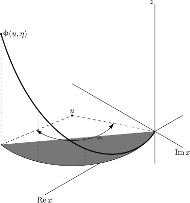
Figure 1: Illustration of the change of coordinates $\Phi$ in the classical Heisenberg group $\mathbb{H}_{1}$. The bold line is a geodesic, whose projection into the $x$-plane is an arc of a circle with center $u$ and subtending an angle $\eta$. The $z$ coordinate of $\Phi(u,\eta)$ is equal to the area of the shaded circular segment.

Note that the $(u,\eta)$ coordinate system omits the set $\{z=0\}=\mathbb{R}^{2n}\times 0\subset G$, for which the arc degenerates into a straight line and has “infinite radius,” as well as the set $\{x=0\}=0\times\mathbb{R}^{m}$, for which the arc becomes a circle whose center $u$ is no longer uniquely determined. These sets are of Haar measure zero and hence will be neglected in the argument without further comment. Estimates which are shown to hold off these sets will also hold on them, by continuity.

$\Phi$ has the property that for each $(u,\eta)$, the path $s\mapsto\Phi(u,s\eta)$ traces the shortest horizontal path between any two of its points, and has constant speed $\left|u\right|\left|\eta\right|$. In particular,

$$d(0,\Phi(u,\eta))=\left|u\right|\left|\eta\right|.$$ (2.22)

Also, for any $f\in C^{1}(G)$,

$$\left|\frac{d}{ds}f(\Phi(u,s\eta))\right|\leq\left|u\right|\left|\eta\right|\left|\nabla f(\Phi(u,s\eta))\right|.$$ (2.23)

Note that if $(x,z)=\Phi(u,\eta)$, we have

$$\left|x\right|^{2} =\left|u\right|^{2}(2-2\cos\left|\eta\right|)$$

$$\left|z\right| =\frac{\left|u\right|^{2}}{2}(\left|\eta\right|-\sin\left|\eta\right|).$$

To compare this with the “polar coordinates” $(u,s)$ used in [3], take $u=u$ and $s=\left|u\right|\eta$.

Let $B:=\{g\in G:d(0,g)<1\}$ denote the unit ball of the Carnot-Carathéodory distance. To express $B$ in $(u,\eta)$ coordinates, we note by (2.22) that $\Phi(u,\eta)\in B$ iff $\left|u\right|\left|\eta\right|\leq 1$; combining this with the constraints on $u$ and $\eta$ given in (2.18), we have

$$B =\left\{\Phi(u,\eta):u\in\mathbb{R}^{2n},\left|\eta\right|<2\pi\wedge\frac{1}{\left|u\right|}\right\}$$ (2.24)

and conversely

$$B^{C} =\left\{\Phi(u,\eta):\left|u\right|\geq\frac{1}{2\pi},\frac{1}{\left|u\right|}\leq\left|\eta\right|<2\pi\right\}$$ (2.25)

modulo the null sets $\{x=0\}$ and $\{z=0\}$, as usual.

In $(u,\eta)$ coordinates, the heat kernel estimate (2.8) reads

$$p_{1}(\Phi(u,\eta)) \asymp\frac{1+(\left|u\right|\left|\eta\right|)^{2n-m-1}}{1+(\left|u\right|^{2}\left|\eta\right|\sqrt{2-2\cos\left|\eta\right|})^{n-\frac{1}{2}}}e^{-\frac{1}{4}(\left|u\right|\left|\eta\right|)^{2}}$$ (2.26)

$$\asymp\frac{1+(\left|u\right|\left|\eta\right|)^{2n-m-1}}{1+\left(\left|u\right|^{2}\left|\eta\right|^{2}(2\pi-\left|\eta\right|)\right)^{n-\frac{1}{2}}}e^{-\frac{1}{4}(\left|u\right|\left|\eta\right|)^{2}}$$ (2.27)

since $1-\cos\theta\asymp\theta^{2}(2\pi-\theta)^{2}$ for $\theta\in[0,2\pi]$. We will often abuse notation and write $p_{1}(u,\eta)$ for $p_{1}(\Phi(u,\eta))$, when no confusion will result.

3 Proof of the gradient estimate

We now begin the proof of Theorem 2.4, which occupies the rest of this article.

We begin by computing the Jacobian determinant of the change of coordinates $\Phi$, so that we can use $(u,\eta)$ coordinates in explicit computations.

Lemma 3.1.

Let $A(u,\eta)$ denote the Jacobian determinant of $\Phi$, so that $dm=A(u,\eta)\,du\,d\eta$. Then

$$A(u,\eta)=\left|u\right|^{2m}\left(\frac{1}{2}-\frac{\sin\left|\eta\right|}{2\left|\eta\right|}\right)^{m-1}(2-2\cos\left|\eta\right|)^{n-1}\left(2-2\cos\left|\eta\right|-\left|\eta\right|\sin\left|\eta\right|\right).$$ (3.1)

Note that $A(u,\eta)$ depends on $u,\eta$ only through their absolute values $\left|u\right|,\left|\eta\right|$. By an abuse of notation we may occasionally use $A$ with $u$ or $\eta$ replaced by scalars, so that $A(r,\rho)$ means $A(r\hat{u},\rho\hat{\eta})$ for arbitrary unit vectors $\hat{u},\hat{\eta}$.

For the Heisenberg group $\mathbb{H}_{1}$ with $n=m=1$, this reduces to

$$A(u,\eta)=\left|u\right|^{2}\left(2-2\cos\left|\eta\right|-\left|\eta\right|\sin\left|\eta\right|\right).$$

The analogous expression appearing in [3] is slightly incorrect. However, it does have the same asymptotics as the correct expression (see Corollary 3.2), which is sufficient for the rest of the argument in [3], so that its overall correctness is not affected.

Proof.

Fix $u,\eta$. Form an orthonormal basis for $T_{(u,\eta)}\Phi^{-1}(G)\cong\mathbb{R}^{2n+m}$ as follows. Let $\hat{u}$ be a unit vector in the direction of $(u,0)$, $\hat{v}$ a unit vector in the direction of $(J_{\eta}u,0)$. For $i=1,\dots,n-1$ let $\hat{w}_{i},\hat{y}_{i}\in\mathbb{R}^{2n}\times 0$ be unit vectors such that $\hat{w}_{i}$ is orthogonal to $\hat{u},\hat{v},\hat{w}_{j},\hat{y}_{j},1\leq j<i$, and let $\hat{y}_{i}$ be in the direction of $J_{\eta}\hat{w}_{i}$ so that $\hat{y}_{i}$ is orthogonal to $\hat{u},\hat{v},\hat{w}_{j},\hat{y}_{j},1\leq j<i$ as well as to $\hat{w}_{i}$. (To see this, note that if $\left\langle x,y\right\rangle=0$ and $\left\langle x,J_{z}y\right\rangle=0$, then $\left\langle J_{z}x,y\right\rangle=0$ and $\left\langle J_{z}x,J_{z}y\right\rangle=-\left|z\right|^{2}\left\langle x,y\right\rangle=0$.) Let $\hat{\eta}$ be a unit vector in the direction of $(0,\eta)$, and let $\hat{\zeta}_{k},k=1,\dots,m-1$ be orthonormal vectors in $0\times\mathbb{R}^{m}$ which are orthogonal to $\hat{\eta}$. Then $\{\hat{u},\hat{v},\hat{w}_{i},\hat{y}_{i},\hat{\eta},\hat{\zeta}_{k}\}$ form an orthonormal basis for $\mathbb{R}^{2n+m}$. Note $J_{\eta}\hat{u}=\left|\eta\right|\hat{v}$, $J_{\eta}\hat{v}=-\left|\eta\right|\hat{u}$,$J_{\eta}\hat{w}_{i}=\left|\eta\right|\hat{y}_{i}$, $J_{\eta}\hat{y}_{i}=-\left|\eta\right|\hat{w}_{i}$. Then

$$\partial_{\hat{u}}\Phi(u,\eta) =(1-\cos\left|\eta\right|)\hat{u}+\sin\left|\eta\right|\hat{v}+\left|u\right|\left(\left|\eta\right|-\sin\left|\eta\right|\right)\hat{\eta}$$

$$\partial_{\hat{v}}\Phi(u,\eta) =(1-\cos\left|\eta\right|)\hat{v}-\sin\left|\eta\right|\hat{u}$$

$$\partial_{\hat{w}_{i}}\Phi(u,\eta) =(1-\cos\left|\eta\right|)\hat{w}_{i}+\sin\left|\eta\right|\hat{y}_{i}$$

$$\partial_{\hat{y}_{i}}\Phi(u,\eta) =(1-\cos\left|\eta\right|)\hat{y}_{i}-\sin\left|\eta\right|\hat{w}_{i}$$

$$\partial_{\hat{\eta}}\Phi(u,\eta) =\left|u\right|(\sin\left|\eta\right|)\hat{u}+\left|u\right|(\cos\left|\eta\right|)\hat{v}+\frac{\left|u\right|^{2}}{2}\left(1-\cos\left|\eta\right|\right)\hat{\eta}$$

$$\partial_{\hat{\zeta}_{k}}\Phi(u,\eta) =\frac{\sin{\left|\eta\right|}}{\left|\eta\right|}J_{\hat{\zeta}_{k}}u+\frac{\left|u\right|^{2}}{2}\left(1-\frac{\sin\left|\eta\right|}{\left|\eta\right|}\right)\hat{\zeta}_{k}.$$

In this basis, the Jacobian matrix has the form

$$J =\begin{pmatrix}1-\cos\left|\eta\right|&-\sin\left|\eta\right|&0&\left|u\right|\sin\left|\eta\right|&0\\ \sin\left|\eta\right|&1-\cos\left|\eta\right|&0&\left|u\right|\cos\left|\eta\right|&0\\ 0&0&B&0&*\\ \left|u\right|(\left|\eta\right|-\sin\left|\eta\right|)&0&0&\frac{\left|u\right|^{2}}{2}(1-\cos\left|\eta\right|)&0\\ 0&0&0&0&D\end{pmatrix}_{(2n+m)\times(2n+m)}$$ (3.2)

where

$$B :=\begin{pmatrix}1-\cos\left|\eta\right|&-\sin\left|\eta\right|&&&\\ \sin\left|\eta\right|&1-\cos\left|\eta\right|&&&\\ &&\ddots&&\\ &&&1-\cos\left|\eta\right|&-\sin\left|\eta\right|\\ &&&\sin\left|\eta\right|&1-\cos\left|\eta\right|\end{pmatrix}_{2(n-1)\times 2(n-1)}$$ (3.3)

is a block-diagonal matrix of $$2\times 2$$ blocks, and

$$D :=\begin{pmatrix}\frac{\left|u\right|^{2}}{2}\left(1-\frac{\sin\left|\eta\right|}{\left|\eta\right|}\right)&&\\ &\ddots&\\ &&\frac{\left|u\right|^{2}}{2}\left(1-\frac{\sin\left|\eta\right|}{\left|\eta\right|}\right)\end{pmatrix}_{(m-1)\times(m-1)}$$ (3.4)

is diagonal. Note $\left|B\right|=(2-2\cos\left|\eta\right|)^{n-1}$ and $\left|D\right|=\left(\frac{\left|u\right|^{2}}{2}\left(1-\frac{\sin\left|\eta\right|}{\left|\eta\right|}\right)\right)^{m-1}$.

So factoring out $\left|D\right|$ and expanding about the $\hat{\eta}$ row, we have

$$\left|J\right| =\left|D\right|\left(\left|u\right|(\left|\eta\right|-\sin\left|\eta\right|)\begin{vmatrix}-\sin\left|\eta\right|&0&\left|u\right|\sin\left|\eta\right|\\ 1-\cos\left|\eta\right|&0&\left|u\right|\cos\left|\eta\right|\\ 0&B&0\end{vmatrix}+\frac{\left|u\right|^{2}}{2}(1-\cos\left|\eta\right|)\begin{vmatrix}1-\cos\left|\eta\right|&-\sin\left|\eta\right|&0\\ \sin\left|\eta\right|&1-\cos\left|\eta\right|&0\\ 0&0&B\end{vmatrix}\right)$$

$$=\left(\frac{\left|u\right|^{2}}{2}\left(1-\frac{\sin\left|\eta\right|}{\left|\eta\right|}\right)\right)^{m-1}$$

$$\quad\times\left(\left|u\right|(\left|\eta\right|-\sin\left|\eta\right|)(-\left|u\right|\sin\left|\eta\right|)(2-2\cos\left|\eta\right|)^{n-1}+\frac{\left|u\right|^{2}}{2}(1-\cos\left|\eta\right|)(2-2\cos\left|\eta\right|)^{n}\right)$$

$$=\left(\frac{\left|u\right|^{2}}{2}\left(1-\frac{\sin\left|\eta\right|}{\left|\eta\right|}\right)\right)^{m-1}\left|u\right|^{2}(2-2\cos\left|\eta\right|)^{n-1}\left((\left|\eta\right|-\sin\left|\eta\right|)(-\sin\left|\eta\right|)+(1-\cos\left|\eta\right|)^{2}\right)$$

$$=\left|u\right|^{2m}\left(\frac{1}{2}-\frac{\sin\left|\eta\right|}{2\left|\eta\right|}\right)^{m-1}(2-2\cos\left|\eta\right|)^{n-1}\left(2-2\cos\left|\eta\right|-\left|\eta\right|\sin\left|\eta\right|\right)$$

∎

Corollary 3.2.

$$A(u,\eta)\asymp\left|u\right|^{2m}\left|\eta\right|^{2(m+n)}(2\pi-\left|\eta\right|)^{2n-1}$$ (3.5)

Proof.

The asymptotic equivalence near $\left|\eta\right|=0$ and $\left|\eta\right|=2\pi$ follows from a routine Taylor series computation.

It then suffices to show that $A(u,\eta)>0$ for all $0<\left|\eta\right|<2\pi$. We have $\frac{1}{2}-\frac{\sin\left|\eta\right|}{2\left|\eta\right|}>0$ for all $\left|\eta\right|>0$, since $x>\sin x$ for all $x>0$. We also have $2-2\cos\left|\eta\right|>0$ for all $0<\left|\eta\right|<2\pi$.

Finally, to show $f(\left|\eta\right|):=2-2\cos\left|\eta\right|-\left|\eta\right|\sin\left|\eta\right|>0$, let $\theta=\frac{1}{2}\left|\eta\right|$. Using double-angle identities, we have $f(2\theta)=4\sin\theta(\sin\theta-\theta\cos\theta)$. For $0<\theta<\pi$ we have $\sin\theta>0$ so it suffices to show $g(\theta):=\sin\theta-\theta\cos\theta>0$. But we have $g(0)=0$ and $g^{\prime}(\theta)=\theta\sin\theta>0$ for $0<\theta<\pi$. ∎

The heat kernel estimates will be used to prove a technical lemma regarding integrating the heat kernel along a geodesic. The proof requires the following simple fact from calculus, of which a close relative appears in [6].

Lemma 3.3.

For any $q\in\mathbb{R}$, $a_{0}>0$ there exists a constant $C=C_{q,a_{0}}$ such that for any $a\geq a_{0}$ we have

$$\int_{t=1}^{t=\infty}t^{q}e^{-(at)^{2}}\,dt\leq C\frac{1}{a^{2}}e^{-a^{2}}.$$ (3.6)

Proof.

Make the change of variables $s=t^{2}$ to get

$$\int_{t=1}^{t=\infty}t^{q}e^{-(at)^{2}}\,dt=\frac{1}{2}\int_{s=1}^{s=\infty}s^{q^{\prime}}e^{-a^{2}s}\,ds$$

where $q^{\prime}=\frac{q-1}{2}$. For $q^{\prime}\leq 0$ (i.e. $q\leq 1$), we have $s^{q^{\prime}}\leq 1$ and thus

$$\int_{s=1}^{s=\infty}s^{q^{\prime}}e^{-a^{2}s}\,ds\leq\int_{s=1}^{s=\infty}e^{-a^{2}s}\,ds=\frac{1}{a^{2}}e^{-a^{2}}.$$

For $q^{\prime}>0$, notice that integration by parts gives

$$\int_{s=1}^{s=\infty}s^{q^{\prime}}e^{-a^{2}s}\,ds =\frac{1}{a^{2}}e^{-a^{2}}+\frac{q^{\prime}}{a^{2}}\int_{s=1}^{s=\infty}s^{q^{\prime}-1}e^{-a^{2}s}\,ds$$

$$\leq\frac{1}{a^{2}}e^{-a^{2}}+\frac{q^{\prime}}{a_{0}^{2}}\int_{s=1}^{s=\infty}s^{q^{\prime}-1}e^{-a^{2}s}\,ds$$

whereupon the result follows by induction. ∎

Lemma 3.4.

For each $q\in\mathbb{R}$ there exists a constant $C_{q}$ such that for all $u,\eta$ with $\Phi(u,\eta)\in B^{C}$, i.e. $\left|u\right|\left|\eta\right|\geq 1$, we have

$$\int_{t=1}^{t=\frac{2\pi}{\left|\eta\right|}}p_{1}(u,t\eta)A(u,t\eta)t^{q}\,dt \leq\frac{C_{q}}{(\left|u\right|\left|\eta\right|)^{2}}p_{1}(u,\eta)A(u,\eta)$$ (3.7)

$$\leq C_{q}p_{1}(u,\eta)A(u,\eta).$$ (3.8)

Note that (3.8) follows immediately from the stronger statement (3.7), since by assumption $\left|u\right|\left|\eta\right|\geq 1$. In fact, we shall only use (3.8) in the sequel.

Proof.

Assume throughout that $\left|u\right|\left|\eta\right|\geq 1$ and $0<\left|\eta\right|<2\pi$. (See (2.25).)

The proof involves the fact that a geodesic passes through (up to) three regions of $G$ in which the estimates for $p_{1}$ and $A$ simplify in different ways. We define these regions, which partition $B^{C}$, as follows. See Figure 2.

Figure 2: The regions $R_{1},R_{2},R_{3}$, seen in the $\left|u\right|$-$\left|\eta\right|$ plane. The dark lines indicate examples of the geodesic paths of integration used in (3.7).

1. Region $R_{1}$ is the set of $\Phi(u,\eta)$ such that $0<\left|\eta\right|\leq\pi$. (This corresponds to having $\left|x\right|^{2}\lesssim\left|z\right|$.) In this region we have $\left|u\right|\geq\frac{1}{\pi}$ and $\pi\leq 2\pi-\left|\eta\right|<2\pi$. Therefore (2.27) becomes

   $$p_{1}(u,\eta) \overset{R_{1}}{\asymp}(\left|u\right|\left|\eta\right|)^{-m}e^{-\frac{1}{4}(\left|u\right|\left|\eta\right|)^{2}}$$

   and Corollary 3.2 yields

   $$A(u,\eta) \overset{R_{1}}{\asymp}\left|u\right|^{2m}\left|\eta\right|^{2(n+m)}$$

   so that

   $$p_{1}(u,\eta)A(u,\eta) \overset{R_{1}}{\asymp}\left|u\right|^{m}\left|\eta\right|^{2n+m}e^{-\frac{1}{4}(\left|u\right|\left|\eta\right|)^{2}}=:F_{1}(u,\eta).$$

2. Region $R_{2}$ is the set of $\Phi(u,\eta)$ such that $\pi<\left|\eta\right|\leq 2\pi-\frac{1}{\left|u\right|^{2}}$. (This corresponds to having $\left|x\right|^{2}\gtrsim\left|z\right|$ and $\left|x\right|^{2}\left|z\right|\gtrsim 1$.) In this region, we have $\left|u\right|^{2}\left|\eta\right|^{2}(2\pi-\left|\eta\right|)\geq\pi^{2}$, so that

   $$p_{1}(u,\eta) \overset{R_{2}}{\asymp}\left|u\right|^{-m}(2\pi-\left|\eta\right|)^{-n+\frac{1}{2}}e^{-\frac{1}{4}(\left|u\right|\left|\eta\right|)^{2}}$$

   $$A(u,\eta) \overset{R_{2}}{\asymp}\left|u\right|^{2m}(2\pi-\left|\eta\right|)^{2n-1}$$

   $$p_{1}(u,\eta)A(u,\eta) \overset{R_{2}}{\asymp}\left|u\right|^{m}(2\pi-\left|\eta\right|)^{n-\frac{1}{2}}e^{-\frac{1}{4}(\left|u\right|\left|\eta\right|)^{2}}=:F_{2}(u,\eta)$$

   $$\overset{R_{2}}{\asymp}\left|u\right|^{m}\left|\eta\right|^{2n+m}(2\pi-\left|\eta\right|)^{n-\frac{1}{2}}e^{-\frac{1}{4}(\left|u\right|\left|\eta\right|)^{2}}=:\tilde{F}_{2}(u,\eta).$$

   We shall use the estimates $F_{2},\tilde{F}_{2}$ at different times. Although $F_{2}\overset{R_{2}}{\asymp}\tilde{F}_{2}$ (since $\left|\eta\right|\overset{R_{2}}{\asymp}1$), they are not equivalent on $R_{1}$.

3. Region $R_{3}$ is the set of $\Phi(u,\eta)$ such that $\left|\eta\right|>\max\left(\pi,2\pi-\frac{1}{\left|u\right|^{2}}\right)$. (This corresponds to having $\left|x\right|^{2}\gtrsim\left|z\right|$ and $\left|x\right|^{2}\left|z\right|\lesssim 1$.) In this region, we have $\left|u\right|^{2}\left|\eta\right|^{2}(2\pi-\left|\eta\right|)<(2\pi)^{2}$, so that

   $$p_{1}(u,\eta) \overset{R_{3}}{\asymp}\left|u\right|^{2n-m-1}e^{-\frac{1}{4}(\left|u\right|\left|\eta\right|)^{2}}$$

   $$A(u,\eta) \overset{R_{3}}{\asymp}\left|u\right|^{2m}(2\pi-\left|\eta\right|)^{2n-1}$$

   $$p_{1}(u,\eta)A(u,\eta) \overset{R_{3}}{\asymp}\left|u\right|^{2n+m-1}(2\pi-\left|\eta\right|)^{2n-1}e^{-\frac{1}{4}(\left|u\right|\left|\eta\right|)^{2}}=:F_{3}(u,\eta)$$

We observe that a geodesic starting from the origin (given by $t\mapsto\Phi(u,t\eta)$ for some fixed $(u,\eta)$) passes through these regions in order, except that it skips Region 2 if $\left|u\right|<\pi^{-1/2}$.

We now estimate the desired integral along a portion of a geodesic lying in a single region.

Claim 3.5.

Let $q\in\mathbb{R}$. Suppose that $F:G\to\mathbb{R}$ is given by

$$F(u,\eta)=\left|u\right|^{\alpha}\left|\eta\right|^{\beta}(2\pi-\left|\eta\right|)^{\gamma}e^{-\frac{1}{4}(\left|u\right|\left|\eta\right|)^{2}}$$

for some nonnegative powers $\alpha,\beta,\gamma$, and that there is some region $R\subset G$ such that $F\overset{R}{\asymp}p_{1}A$. Then there is a constant $C$ depending on $q$, $F$, $R$ such that for all $u,\eta,\tau_{0},\tau_{1},\tau_{2}$ satisfying

• $\left|u\right|\left|\eta\right|\geq 1$;

• $1\leq\tau_{0}\leq\tau_{1}\leq\tau_{2}\leq\frac{2\pi}{\left|\eta\right|}$; and

• $\Phi(u,t\eta)\in R$ for all $t\in[\tau_{1},\tau_{2}]$

we have

$$\int_{t=\tau_{1}}^{t=\tau_{2}}p_{1}(u,t\eta)A(u,t\eta)t^{q}\,dt\leq C\frac{\tau_{0}^{q-1}}{(\left|u\right|\left|\eta\right|)^{2}}F(u,\tau_{0}\eta).$$ (3.9)

Proof of Claim 3.5.

We have

$$\int_{t=\tau_{1}}^{t=\tau_{2}}p_{1}(u,t\eta)A(u,t\eta)t^{q}\,dt \leq C\int_{t=\tau_{1}}^{t=\tau_{2}}F(u,t\eta)t^{q}\,dt$$

$$\leq C\int_{t=\tau_{0}}^{t=\tau_{2}}F(u,t\eta)t^{q}\,dt$$

$$=C\left|u\right|^{\alpha}\left|\eta\right|^{\beta}\int_{t=\tau_{0}}^{t=\tau_{2}}t^{q+\beta}(2\pi-t\left|\eta\right|)^{\gamma}e^{-\frac{1}{4}(t\left|u\right|\left|\eta\right|)^{2}}\,dt$$

$$\leq C\left|u\right|^{\alpha}\left|\eta\right|^{\beta}(2\pi-\tau_{0}\left|\eta\right|)^{\gamma}\int_{t=\tau_{0}}^{t=\tau_{2}}t^{q+\beta}e^{-\frac{1}{4}(t\left|u\right|\left|\eta\right|)^{2}}\,dt$$

since $$t\geq\tau_{0} t=t^{\prime}\tau_{0}$$. We now make the change of variables :

$$\leq C\left|u\right|^{\alpha}\left|\eta\right|^{\beta}(2\pi-\tau_{0}\left|\eta\right|)^{\gamma}\tau_{0}^{q+\beta+1}\int_{t^{\prime}=1}^{t^{\prime}=\infty}t^{\prime q+\beta}e^{-\frac{1}{4}(t^{\prime}\tau_{0}\left|u\right|\left|\eta\right|)^{2}}\,dt^{\prime}$$

$$\leq C^{\prime}\left|u\right|^{\alpha}\left|\eta\right|^{\beta}(2\pi-\tau_{0}\left|\eta\right|)^{\gamma}\tau_{0}^{q+\beta+1}\frac{1}{(\tau_{0}\left|u\right|\left|\eta\right|)^{2}}e^{-\frac{1}{4}(\tau_{0}\left|u\right|\left|\eta\right|)^{2}}$$

$$=C^{\prime}\frac{\tau_{0}^{q-1}}{(\left|u\right|\left|\eta\right|)^{2}}F(u,\tau_{0}\eta)$$

where in the second-to-last line we applied Lemma 3.3 with $a=\frac{1}{2}\tau_{0}\left|u\right|\left|\eta\right|$, $a_{0}=\frac{1}{2}$. (Note that $\left|u\right|\left|\eta\right|\geq 1$ and $\tau_{0}\geq 1$ by assumption, so $a\geq a_{0}$.) Claim 3.5 is proved. ∎

Now for fixed $u,\eta$, let

$$t_{2} :=\max\left(1,\frac{\pi}{\left|\eta\right|}\right)$$

$$t_{3} :=\max\left(t_{2},\frac{1}{\left|\eta\right|}\left(2\pi-\frac{1}{\left|u\right|^{2}}\right)\right)$$

so that

$$\Phi(u,t\eta) \in R_{1}\text{ for }1<t\leq t_{2}$$

$$\Phi(u,t\eta) \in R_{2}\text{ for }t_{2}<t<t_{3}$$

$$\Phi(u,t\eta) \in R_{3}\text{ for }t_{3}\leq t<\frac{2\pi}{\left|\eta\right|}.$$

We divide the remainder of the proof into cases, depending on the region where $\Phi(u,\eta)$ resides.

Case 1.

Suppose that $\Phi(u,\eta)\in R_{1}$. We have

$$\int_{t=1}^{t=\frac{2\pi}{\left|\eta\right|}}p_{1}(u,t\eta)A(u,t\eta)t^{q}\,dt=\int_{t=1}^{t=t_{2}}+\int_{t=t_{2}}^{t=t_{3}}+\int_{t=t_{3}}^{t=\frac{2\pi}{\left|\eta\right|}}.$$

For the first integral, where $\Phi(u,t\eta)\in R_{1}$, we have by Claim 3.5 (taking $\tau_{0}=\tau_{1}=1$, $\tau_{2}=t_{2}$, $R=R_{1}$, $F=F_{1}$) that

$$\int_{t=1}^{t=t_{2}}p_{1}(u,t\eta)A(u,t\eta)t^{q}\,dt\leq\frac{C}{(\left|u\right|\left|\eta\right|)^{2}}F_{1}(u,\eta)\leq\frac{C^{\prime}}{(\left|u\right|\left|\eta\right|)^{2}}p_{1}(u,\eta)A(u,\eta)$$

since $F_{1}\overset{R_{1}}{\asymp}p_{1}A$.

For the second integral, where $\Phi(u,t\eta)\in R_{2}$, we take $\tau_{0}=1$, $\tau_{1}=t_{2}$, $\tau_{2}=t_{3}$, $R=R_{2}$, $F=\tilde{F}_{2}$ in Claim 3.5 to obtain

$$\int_{t=t_{2}}^{t=t_{3}}p_{1}(u,t\eta)A(u,t\eta)t^{q}\,dt \leq\frac{C}{(\left|u\right|\left|\eta\right|)^{2}}\tilde{F}_{2}(u,\eta).$$

However, for $\Phi(u,\eta)\in R_{1}$ we have

$$\frac{\tilde{F}_{2}(u,\eta)}{F_{1}(u,\eta)}=(2\pi-\left|\eta\right|)^{n-\frac{1}{2}}\leq(2\pi)^{n-\frac{1}{2}}.$$

Thus

$$\int_{t=t_{2}}^{t=t_{3}}p_{1}(u,t\eta)A(u,t\eta)t^{q}\,dt \leq\frac{C^{\prime}}{(\left|u\right|\left|\eta\right|)^{2}}{F}_{1}(u,\eta)$$

$$\leq\frac{C^{\prime\prime}}{(\left|u\right|\left|\eta\right|)^{2}}p_{1}(u,\eta)A(u,\eta)$$

The third integral is more subtle. We apply Claim 3.5 with $\tau_{0}=\tau_{1}=t_{3}$, $\tau_{3}=\frac{2\pi}{\left|\eta\right|}$, $R=R_{3}$, $F={F}_{3}$:

$$\int_{t=t_{3}}^{t=\frac{2\pi}{\left|\eta\right|}}p_{1}(u,t\eta)A(u,t\eta)t^{q}\,dt \leq C\frac{t_{3}^{q-1}}{(\left|u\right|\left|\eta\right|)^{2}}{F}_{3}(u,t_{3}\eta)$$

Then

$$\frac{t_{3}^{q-1}{F}_{3}(u,t_{3}\eta)}{F_{1}(u,\eta)} =t_{3}^{q-1}\left|u\right|^{2n-1}\left|\eta\right|^{-2n-m}(2\pi-t_{3}\left|\eta\right|)^{2n-1}e^{-\frac{1}{4}(\left|u\right|\left|\eta\right|)^{2}(t_{3}^{2}-1)}.$$ (3.10)

We must show that this ratio is bounded. Fix some $\epsilon>0$. If $\left|u\right|\geq(\pi-\epsilon)^{-1/2}>\pi^{-1/2}$, we have $2\pi-\frac{1}{\left|u\right|^{2}}>\pi+\epsilon$ and thus $t_{3}=\frac{1}{\left|\eta\right|}\left(2\pi-\frac{1}{\left|u\right|^{2}}\right)$. Then

$$\left|\eta\right|^{2}(t_{3}^{2}-1) =\left(2\pi-\frac{1}{\left|u\right|^{2}}\right)^{2}-\left|\eta\right|^{2}$$

$$\geq(\pi+\epsilon)^{2}-\pi^{2}=2\pi\epsilon+\epsilon^{2}.$$

So in this case (3.10) becomes

$$\frac{t_{3}^{q-1}{F}_{3}(u,t_{3}\eta)}{F_{1}(u,\eta)} =\left(\frac{1}{\left|\eta\right|}\left(2\pi-\frac{1}{\left|u\right|^{2}}\right)\right)^{q-1}\left|u\right|^{2n-1}\left|\eta\right|^{-2n-m}\left(\frac{1}{\left|u\right|^{2}}\right)^{2n-1}e^{-\frac{1}{4}(\left|u\right|\left|\eta\right|)^{2}(t_{3}^{2}-1)}$$

$$=\left(2\pi-\frac{1}{\left|u\right|^{2}}\right)^{q-1}\left|u\right|^{-2n+1}\left|\eta\right|^{-2n-m-q+1}e^{-\frac{1}{4}(\left|u\right|\left|\eta\right|)^{2}(t_{3}^{2}-1)}$$

$$\leq(2\pi)^{q-1}\left|u\right|^{m+q}e^{-\frac{1}{4}(2\pi\epsilon+\epsilon^{2})\left|u\right|^{2}}$$

since $\left|\eta\right|\leq\frac{1}{\left|u\right|}$. This is certainly bounded by some constant. On the other hand, if $\left|u\right|\leq(\pi-\epsilon)^{-1/2}$, then $\left|\eta\right|\geq(\pi-\epsilon)^{1/2}$ and $1\leq t_{3}\leq\left(\frac{\pi+\epsilon}{\pi-\epsilon}\right)^{1/2}$, so that the right side of (3.10) is clearly bounded.

Thus we have

$$\int_{t=t_{3}}^{t=\frac{2\pi}{\left|\eta\right|}}p_{1}(u,t\eta)A(u,t\eta)t^{q}\,dt \leq\frac{C^{\prime}}{(\left|u\right|\left|\eta\right|)^{2}}{F}_{1}(u,\eta)$$

$$\leq\frac{C^{\prime\prime}}{(\left|u\right|\left|\eta\right|)^{2}}p_{1}(u,\eta)A(u,\eta)$$

This completes the proof of this case.

Case 2.

Suppose that $\Phi(u,\eta)\in R_{2}$. We have

$$\int_{t=1}^{t=\frac{2\pi}{\left|\eta\right|}}p_{1}(u,t\eta)A(u,t\eta)t^{q}\,dt=\int_{t=1}^{t=t_{3}}+\int_{t=t_{3}}^{t=\frac{2\pi}{\left|\eta\right|}}.$$

Note that in this region we have $1\leq t_{3}\leq 2$. Again by Claim 3.5, with $\tau_{0}=\tau_{1}=1$ and $\tau_{2}=t_{3}$, we have

$$\int_{t=1}^{t=t_{3}}p_{1}(u,t\eta)A(u,t\eta)t^{q}\,dt\leq\frac{C}{(\left|u\right|\left|\eta\right|)^{2}}F_{2}(u,\eta)\leq\frac{C^{\prime}}{(\left|u\right|\left|\eta\right|)^{2}}p_{1}(u,\eta)A(u,\eta).$$

For the second integral, we apply Claim 3.5 with $\tau_{0}=1$, $\tau_{1}=t_{3}$, $\tau_{2}=\frac{2\pi}{\left|\eta\right|}$ to get

$$\int_{t=t_{3}}^{t=\frac{2\pi}{\left|\eta\right|}}p_{1}(u,t\eta)A(u,t\eta)t^{q}\,dt \leq\frac{C}{(\left|u\right|\left|\eta\right|)^{2}}F_{3}(u,\eta).$$

But $\left|\eta\right|\geq 2\pi-\frac{1}{\left|u\right|^{2}}$ on $R_{3}$, so we have

$$\frac{F_{3}(u,\eta)}{F_{2}(u,\eta)} =\left|u\right|^{2n-1}(2\pi-\left|\eta\right|)^{n-\frac{1}{2}}$$

$$\leq\left|u\right|^{2n-1}\left(\frac{1}{\left|u\right|^{2}}\right)^{n-\frac{1}{2}}=1.$$

Thus

$$\int_{t=t_{3}}^{t=\frac{2\pi}{\left|\eta\right|}}p_{1}(u,t\eta)A(u,t\eta)t^{q}\,dt \leq\frac{C^{\prime}}{(\left|u\right|\left|\eta\right|)^{2}}{F}_{2}(u,\eta)$$

$$\leq\frac{C^{\prime\prime}}{(\left|u\right|\left|\eta\right|)^{2}}p_{1}(u,\eta)A(u,\eta).$$

Case 3.

Suppose $\Phi(u,\eta)\in R_{3}$; we apply Claim 3.5 with $\tau_{0}=\tau_{1}=1$, $\tau_{2}=\frac{2\pi}{\left|\eta\right|}$ to get

$$\int_{t=1}^{t=\frac{2\pi}{\left|\eta\right|}}p_{1}(u,t\eta)A(u,t\eta)t^{q}\,dt\leq C\frac{1}{(\left|u\right|\left|\eta\right|)^{2}}F_{3}(u,\eta)\leq C^{\prime}p_{1}(u,\eta)A(u,\eta).$$

The three cases together complete the proof of Lemma 3.4. ∎

Notation 3.6.

For $f\in C^{1}(G)$, let $m_{f}:=\frac{\int_{B}f\,dm}{\int_{B}dm}$, where $B$ is the Carnot-Carathéodory unit ball. .

To continue to follow the line of [3], we need the following Poincaré inequality. This theorem can be found in [8], and is a special case of a more general theorem appearing in [12].

Theorem 3.7.

There exists a constant $C$ such that for any $f\in C^{\infty}(G)$,

$$\int_{B}\left|f-m_{f}\right|\,dm\leq C\int_{B}\left|\nabla f\right|\,dm.$$ (3.11)

Corollary 3.8.

There exists a constant $C$ such that for any $f\in C^{\infty}(G)$,

$$\int_{B}\left|f-m_{f}\right|p_{1}\,dm\leq C\int_{B}\left|\nabla f\right|p_{1}\,dm.$$ (3.12)

Proof.

$p_{1}$ is bounded and bounded below away from $0$ on $B$. ∎

Lemma 3.9 (akin to Lemma 5.2 of [3]).

There exists a constant $C$ such that for all $f\in\mathcal{C}$,

$$\int_{B^{C}}\left|f-m_{f}\right|p_{1}\,dm\leq C\int_{G}\left|\nabla f\right|p_{1}\,dm.$$ (3.13)

Proof.

Changing to $(u,\eta)$ coordinates, we wish to show

$$\int_{\left|u\right|\geq\frac{1}{2\pi}}\int_{\frac{1}{\left|u\right|}\leq\left|\eta\right|<2\pi}\left|f(\Phi(u,\eta))-m_{f}\right|p_{1}(\Phi(u,\eta))A(u,\eta)\,d\eta\,du\leq C\int_{G}\left|\nabla f\right|p_{1}\,dm.$$ (3.14)

(The limits of integration are as described in (2.25).) By an abuse of notation we shall write $f(u,\eta)$ for $f(\Phi(u,\eta))$, $p_{1}(u,\eta)$ for $p_{1}(\Phi(u,\eta))$, $\nabla f(u,\eta)$ for $(\nabla f)(\Phi(u,\eta))$, et cetera.

Let $g(u,\eta):=f\left(u,\min\left(\left|\eta\right|,\frac{1}{\left|u\right|}\right)\frac{\eta}{\left|\eta\right|}\right)$. Then $g=f$ on $B$ (in particular $m_{g}=m_{f}$), $g$ is bounded, the function $s\mapsto g(u,s\eta)$ is absolutely continuous, and $\frac{d}{ds}g(u,s\eta)=0$ for $s>\frac{1}{\left|u\right|\left|\eta\right|}$.

Now $\left|f-m_{f}\right|\leq\left|f-g\right|+\left|g-m_{f}\right|$. We first observe that for $\left|u\right|\left|\eta\right|\geq 1$ we have

$$\left|f(u,\eta)-g(u,\eta)\right| =\left|\int_{s=\frac{1}{\left|u\right|\left|\eta\right|}}^{s=1}\left(\frac{d}{ds}f(u,s\eta)-\cancel{\frac{d}{ds}g(u,s\eta)}\right)\,ds\right|$$

$$\leq\int_{s=\frac{1}{\left|u\right|\left|\eta\right|}}^{s=1}\left|\nabla f(u,s\eta)\right|\left|u\right|\left|\eta\right|\,ds$$

by (2.23). Thus

$$\int_{B^{C}}\left|f-g\right|p_{1}\,dm =\int_{\left|u\right|\geq\frac{1}{2\pi}}\int_{\left|\eta\right|\geq\frac{1}{\left|u\right|}}\left|f(u,\eta)-g(u,\eta)\right|p_{1}(u,\eta)A(u,\eta)\,d\eta\,du$$

where the limits of integration come from the conditions $$\left|u\right|\left|\eta\right|\geq 1 \left|\eta\right|<2\pi$$, ;

$$\leq\int_{\left|u\right|\geq\frac{1}{2\pi}}\int_{\left|\eta\right|\geq\frac{1}{\left|u\right|}}\int_{s=\frac{1}{\left|u\right|\left|\eta\right|}}^{s=1}\left|\nabla f(u,s\eta)\right|\left|u\right|\left|\eta\right|p_{1}(u,\eta)A(u,\eta)\,ds\,d\eta\,du$$

$$=\int_{\left|u\right|\geq\frac{1}{2\pi}}\int_{s=0}^{s=1}\int_{\frac{1}{s\left|u\right|}\leq\left|\eta\right|\leq 2\pi}\left|\nabla f(u,s\eta)\right|\left|u\right|\left|\eta\right|p_{1}(u,\eta)A(u,\eta)\,d\eta\,ds\,du$$

by Tonelli’s theorem. We now make the change of variables $$\eta^{\prime}=s\eta$$ to obtain

$$=\int_{\left|u\right|\geq\frac{1}{2\pi}}\int_{s=0}^{s=1}\int_{\frac{1}{\left|u\right|}\leq\left|\eta^{\prime}\right|\leq 2\pi s}\left|\nabla f(u,\eta^{\prime})\right|\left|u\right|\frac{1}{s}\left|\eta^{\prime}\right|p_{1}\left(u,\frac{1}{s}\eta^{\prime}\right)A\left(u,\frac{1}{s}\eta^{\prime}\right)\frac{1}{s^{m}}\,d\eta^{\prime}\,ds\,du$$

$$=\int_{\left|u\right|\geq\frac{1}{2\pi}}\int_{\frac{1}{\left|u\right|}\leq\left|\eta^{\prime}\right|\leq 2\pi}\left|\nabla f(u,\eta^{\prime})\right|\left|u\right|\left|\eta^{\prime}\right|$$

$$\quad\times\left(\int_{s=\frac{\left|\eta^{\prime}\right|}{2\pi}}^{s=1}p_{1}\left(u,\frac{1}{s}\eta^{\prime}\right)A\left(u,\frac{1}{s}\eta^{\prime}\right)\frac{1}{s^{m+1}}\,ds\right)\,d\eta^{\prime}\,du$$

Make the further change of variables $$t=\frac{1}{s}$$ to get

$$=\int_{\left|u\right|\geq\frac{1}{2\pi}}\int_{\frac{1}{\left|u\right|}\leq\left|\eta^{\prime}\right|\leq 2\pi}\left|\nabla f(u,\eta^{\prime})\right|\left|u\right|\left|\eta^{\prime}\right|\left(\int_{t=1}^{t=\frac{2\pi}{\left|\eta^{\prime}\right|}}p_{1}(u,t\eta^{\prime})A(u,t\eta^{\prime})t^{m-1}\,dt\right)\,d\eta^{\prime}\,du.$$

Applying Lemma 3.4 to the bracketed term gives

$$\leq C\int_{\left|u\right|\geq\frac{1}{2\pi}}\int_{\frac{1}{\left|u\right|}\leq\left|\eta^{\prime}\right|\leq 2\pi}\frac{1}{\left|u\right|\left|\eta^{\prime}\right|}\left|\nabla f(u,\eta^{\prime})\right|p_{1}(u,\eta^{\prime})A(u,\eta^{\prime})\,d\eta^{\prime}\,du$$

$$\leq C^{\prime}\int_{B^{C}}\left|\nabla f\right|p_{1}\,dm$$

converting back from geodesic coordinates and using the fact that $\left|u\right|\left|\eta^{\prime}\right|\geq 1$.

To complete the proof, we must show that $\int_{B^{C}}\left|g-m_{f}\right|p_{1}\,dm\leq\int_{G}\left|\nabla f\right|p_{1}\,dm$. Note that for $\Phi(u,\eta)\in B^{C}$, i.e. $\left|u\right|\left|\eta\right|\geq 1$, we have $g(u,\eta)=f\left(u,\frac{1}{\left|u\right|\left|\eta\right|}\eta\right)$, so

$$\int_{B^{C}}\left|g-m_{f}\right|p_{1}\,dm =\int_{\left|u\right|\geq\frac{1}{2\pi}}\int_{\frac{1}{\left|u\right|}\leq\left|\eta\right|\leq 2\pi}\left|f\left(u,\frac{1}{\left|u\right|\left|\eta\right|}\eta\right)-m_{f}\right|p_{1}(u,\eta)A(u,\eta)\,d\eta\,du.$$ (3.15)

Change the $$\eta \eta=\rho\hat{\eta} \rho\geq 0 \left|\hat{\eta}\right|=1 p_{1}(u,\eta),A(u,\eta) \eta \rho \hat{\eta}$$ integral to polar coordinates by writing , where and . Note that depend on only through and not .

$$=C\int_{\left|u\right|\geq\frac{1}{2\pi}}\int_{\hat{\eta}\in S^{m-1}}\left|f\left(u,\frac{1}{\left|u\right|}\hat{\eta}\right)-m_{f}\right|\int_{\rho=\frac{1}{\left|u\right|}}^{\rho=2\pi}p_{1}(u,\rho)A(u,\rho)\rho^{m-1}\,d\rho\,d\hat{\eta}\,du$$ (3.16)

Now, for any $s\in[0,1]$ we have

$$\left|f\left(u,\frac{1}{\left|u\right|}\hat{\eta}\right)-m_{f}\right|\leq\left|f\left(u,\frac{1}{\left|u\right|}\hat{\eta}\right)-f\left(u,\frac{s}{\left|u\right|}\hat{\eta}\right)\right|+\left|f\left(u,\frac{s}{\left|u\right|}\hat{\eta}\right)-m_{f}\right|.$$ (3.17)

Let

$$D(u):=\int_{s=0}^{s=1}\frac{s^{m-1}}{\left|u\right|^{m}}A\left(u,\frac{s}{\left|u\right|}\right)\,ds.$$ (3.18)

By multiplying both sides of (3.17) by $\frac{1}{D(u)}\frac{s^{m-1}}{\left|u\right|^{m}}A\left(u,\frac{s}{\left|u\right|}\right)$ and integrating we obtain

$$\begin{split}\left|f\left(u,\frac{1}{\left|u\right|}\hat{\eta}\right)-m_{f}\right|&\leq\frac{1}{D(u)}\int_{s=0}^{s=1}\left(\left|f\left(u,\frac{1}{\left|u\right|}\hat{\eta}\right)-f\left(u,\frac{s}{\left|u\right|}\hat{\eta}\right)\right|+\left|f\left(u,\frac{s}{\left|u\right|}\hat{\eta}\right)-m_{f}\right|\right)\\ &\quad\times\frac{s^{m-1}}{\left|u\right|^{m}}A\left(u,\frac{s}{\left|u\right|}\right)\,ds.\end{split}$$ (3.19)

Let

$$R(u):=\frac{1}{D(u)}\int_{\rho=\frac{1}{\left|u\right|}}^{\rho=2\pi}p_{1}(u,\rho)A(u,\rho)\rho^{m-1}\,d\rho.$$ (3.20)

Then substituting (3.19) into (3.16) and using (3.20) we have

$$\int_{B^{C}}\left|g-m_{f}\right|p_{1}\,dm\leq I_{1}+I_{2}$$ (3.21)

where

$$I_{1} :=\int_{\left|u\right|\geq\frac{1}{2\pi}}\int_{\hat{\eta}\in S^{m-1}}\int_{s=0}^{s=1}\left|f\left(u,\frac{1}{\left|u\right|}\hat{\eta}\right)-f\left(u,\frac{s}{\left|u\right|}\hat{\eta}\right)\right|\frac{s^{m-1}}{\left|u\right|^{m}}A\left(u,\frac{s}{\left|u\right|}\right)\,ds\,R(u)\,d\hat{\eta}\,du$$ (3.22)

$$I_{2} :=\int_{\left|u\right|\geq\frac{1}{2\pi}}\int_{\hat{\eta}\in S^{m-1}}\int_{s=0}^{s=1}\left|f\left(u,\frac{s}{\left|u\right|}\hat{\eta}\right)-m_{f}\right|\frac{s^{m-1}}{\left|u\right|^{m}}A\left(u,\frac{s}{\left|u\right|}\right)\,ds\,R(u)\,d\hat{\eta}\,du.$$ (3.23)

We now show that $I_{1}$, $I_{2}$ can each be bounded by a constant times $\int_{G}\left|\nabla f\right|p_{1}\,dm$, using the following claim.

Claim 3.10.

There exists a constant $C$ such that for all $\left|u\right|\geq\frac{1}{2\pi}$ we have

$$R(u)\leq C\left(2\pi-\frac{1}{\left|u\right|}\right)^{2n-1}\leq(2\pi)^{2n-1}C.$$ (3.24)

Proof of Claim.

First, by Corollary 3.2 we have

$$D(u) :=\int_{s=0}^{s=1}\frac{s^{m-1}}{\left|u\right|^{m}}A\left(u,\frac{s}{\left|u\right|}\right)\,ds$$

$$\geq C\int_{s=0}^{s=1}\frac{s^{m-1}}{\left|u\right|^{m}}\left|u\right|^{2m}\left(\frac{s}{\left|u\right|}\right)^{2(m+n)}\left(2\pi-\frac{s}{\left|u\right|}\right)^{2n-1}\,ds$$

$$=C\left|u\right|^{-2n-m}\int_{s=0}^{s=1}s^{3m+2n-1}\left(2\pi-\frac{s}{\left|u\right|}\right)^{2n-1}\,ds$$

$$\geq C\left|u\right|^{-2n-m}\int_{s=0}^{s=1}s^{3m+2n-1}\left(2\pi(1-s)\right)^{2n-1}\,ds u\geq\frac{1}{2\pi}$$ since

$$=C^{\prime}\left|u\right|^{-2n-m}$$

since the $s$ integral is a positive constant independent of $u$.

On the other hand, making the change of variables $\rho=\frac{t}{\left|u\right|}$ shows

$$\int_{\rho=\frac{1}{\left|u\right|}}^{\rho=2\pi}p_{1}(u,\rho)A(u,\rho)\rho^{m-1}\,d\rho =\left|u\right|^{-m}\int_{t=1}^{t=2\pi\left|u\right|}p_{1}\left(u,\frac{t}{\left|u\right|}\right)A\left(u,\frac{t}{\left|u\right|}\right)t^{m-1}\,dt$$

$$\leq C\left|u\right|^{-m}p_{1}\left(u,\frac{1}{\left|u\right|}\right)A\left(u,\frac{1}{\left|u\right|}\right)$$

by taking $\left|\eta\right|=\frac{1}{\left|u\right|}$ in Lemma 3.4. Now $p_{1}\left(u,\frac{1}{\left|u\right|}\right)$ is the heat kernel evaluated at a point on the unit sphere of $G$, so this is bounded by a constant independent of $u$. Thus by Corollary 3.2 we have

$$\int_{\rho=\frac{1}{\left|u\right|}}^{\rho=2\pi}p_{1}(u,\rho)A(u,\rho)\rho^{m-1}\,d\rho \leq C\left|u\right|^{-m}\left|u\right|^{2m}\left(\frac{1}{\left|u\right|}\right)^{2(m+n)}\left(2\pi-\frac{1}{\left|u\right|}\right)^{2n-1}$$

$$\leq C\left(2\pi-\frac{1}{\left|u\right|}\right)^{2n-1}\left|u\right|^{-2n-m}.$$

Combining this with the estimate on $D(u)$ proves the claim. ∎

To estimate $I_{1}$ (see (3.22)), we observe that

$$\left|f\left(u,\frac{1}{\left|u\right|}\hat{\eta}\right)-f\left(u,\frac{s}{\left|u\right|}\hat{\eta}\right)\right| =\left|\int_{t=s}^{t=1}\frac{d}{dt}f\left(u,\frac{t}{\left|u\right|}\hat{\eta}\right)\,dt\right|$$

$$\leq\int_{t=s}^{t=1}\left|\frac{d}{dt}f\left(u,\frac{t}{\left|u\right|}\hat{\eta}\right)\right|\,dt$$

$$\leq\int_{t=s}^{t=1}\left|\nabla f\left(u,\frac{t}{\left|u\right|}\hat{\eta}\right)\right|\,dt$$

by (2.23). Thus

$$I_{1} \leq\int_{\left|u\right|\geq\frac{1}{2\pi}}\int_{\hat{\eta}\in S^{m-1}}\int_{s=0}^{s=1}\int_{t=s}^{t=1}\left|\nabla f\left(u,\frac{t}{\left|u\right|}\hat{\eta}\right)\right|\frac{s^{m-1}}{\left|u\right|^{m}}A\left(u,\frac{s}{\left|u\right|}\right)\,dt\,ds\,R(u)\,d\hat{\eta}\,du$$ (3.25)

$$=\int_{\left|u\right|\geq\frac{1}{2\pi}}\int_{\hat{\eta}\in S^{m-1}}\int_{t=0}^{t=1}\left|\nabla f\left(u,\frac{t}{\left|u\right|}\hat{\eta}\right)\right|\frac{1}{\left|u\right|^{m}}\left(R(u)\int_{s=0}^{s=t}s^{m-1}A\left(u,\frac{s}{\left|u\right|}\right)\,ds\right)\,dt\,d\hat{\eta}\,du.$$ (3.26)

Now by Claim 3.10 and Corollary 3.2, we have for all $t\in[0,1]$:

$$R(u)\int_{s=0}^{s=t}s^{m-1}A\left(u,\frac{s}{\left|u\right|}\right)\,ds \leq C\left(2\pi-\frac{1}{\left|u\right|}\right)^{2n-1}\int_{s=0}^{s=t}s^{m-1}\left|u\right|^{2m}\left(\frac{s}{\left|u\right|}\right)^{2(m+n)}\left(2\pi-\frac{s}{\left|u\right|}\right)^{2n-1}\,ds$$

$$\leq C\left(2\pi-\frac{t}{\left|u\right|}\right)^{2n-1}(2\pi)^{2n-1}\left|u\right|^{-2n}\int_{s=0}^{s=t}s^{3m+2n-1}\,ds$$

$$=C^{\prime}\left(2\pi-\frac{t}{\left|u\right|}\right)^{2n-1}\left|u\right|^{-2n}t^{3m+2n}$$

$$=C^{\prime}\left(2\pi-\frac{t}{\left|u\right|}\right)^{2n-1}\left|u\right|^{2m}\left(\frac{t}{\left|u\right|}\right)^{2(m+n)}t^{m}$$

$$\leq C^{\prime\prime}A\left(u,\frac{t}{\left|u\right|}\right)t^{m}$$

$$\leq C^{\prime\prime}A\left(u,\frac{t}{\left|u\right|}\right)t^{m-1}.$$

Thus

$$I_{1} \leq C\int_{\left|u\right|\geq\frac{1}{2\pi}}\int_{\hat{\eta}\in S^{m-1}}\int_{t=0}^{t=1}\left|\nabla f\left(u,\frac{t}{\left|u\right|}\hat{\eta}\right)\right|A\left(u,\frac{t}{\left|u\right|}\right)\frac{t^{m-1}}{\left|u\right|^{m}}\,dt\,d\hat{\eta}\,du$$ (3.27)

Make the change of variables $$r=\frac{t}{\left|u\right|}$$:

$$=C\int_{\left|u\right|\geq\frac{1}{2\pi}}\int_{\hat{\eta}\in S^{m-1}}\int_{r=0}^{r=\frac{1}{\left|u\right|}}\left|\nabla f\left(u,r\hat{\eta}\right)\right|A\left(u,r\right)r^{m-1}\,dr\,d\hat{\eta}\,du$$ (3.28)

$$\leq C\int_{u\in\mathbb{R}^{2n}}\int_{\hat{\eta}\in S^{m-1}}\int_{r=0}^{r=\frac{1}{\left|u\right|}}\left|\nabla f\left(u,r\hat{\eta}\right)\right|A\left(u,r\right)r^{m-1}\,dr\,d\hat{\eta}\,du$$ (3.29)

$$=C\int_{B}\left|\nabla f\right|\,dm$$ (3.30)

$$\leq\frac{C}{\inf_{B}p_{1}}\int_{B}\left|\nabla f\right|p_{1}\,dm$$ (3.31)

$$\leq C^{\prime}\int_{G}\left|\nabla f\right|p_{1}\,dm.$$ (3.32)

where we have used the fact that $p_{1}$ is bounded away from $0$ on $B$.

For $I_{2}$ (see (3.23)), we have by Claim 3.10 that

$$I_{2} \leq C\int_{\left|u\right|\geq\frac{1}{2\pi}}\int_{\hat{\eta}\in S^{m-1}}\int_{s=0}^{s=1}\left|f\left(u,\frac{s}{\left|u\right|}\hat{\eta}\right)-m_{f}\right|\frac{s^{m-1}}{\left|u\right|^{m}}A\left(u,\frac{s}{\left|u\right|}\right)\,ds\,d\hat{\eta}\,du.$$ (3.33)

Make the change of variables $$r=\frac{s}{\left|u\right|}$$:

$$=C\int_{\left|u\right|\geq\frac{1}{2\pi}}\int_{\hat{\eta}\in S^{m-1}}\int_{r=0}^{r=\frac{1}{\left|u\right|}}\left|f\left(u,r\hat{\eta}\right)-m_{f}\right|r^{m-1}A\left(u,r\right)\,dr\,d\hat{\eta}\,du$$ (3.34)

$$\leq C\int_{u\in\mathbb{R}^{2n}}\int_{\hat{\eta}\in S^{m-1}}\int_{r=0}^{r=\frac{1}{\left|u\right|}}\left|f\left(u,r\hat{\eta}\right)-m_{f}\right|r^{m-1}A\left(u,r\right)\,dr\,d\hat{\eta}du$$ (3.35)

$$=C\int_{B}\left|f-m_{f}\right|\,dm$$ (3.36)

$$\leq C\int_{B}\left|\nabla f\right|\,dm$$ (3.37)

by Theorem 3.7. The inequalities (3.30–3.32) now show that $I_{2}\leq C^{\prime}\int_{G}\left|\nabla f\right|p_{1}\,dm$, as desired. ∎

Corollary 3.11.

There exists a constant $C$ such that for all $f\in\mathcal{C}$,

$$\int_{G}\left|f-m_{f}\right|p_{1}\,dm\leq C\int_{G}\left|\nabla f\right|p_{1}\,dm.$$ (3.38)

Proof.

Add (3.12) and (3.13). ∎

We can now prove some cases of the desired gradient inequality (2.16).

Notation 3.12.

Let $D(R)=\{(x,z):\left|x\right|\leq R\}$ denote the “cylinder about the $z$ axis” of radius $R$.

Lemma 3.13.

For fixed $R>0$, (2.16) holds, with a constant $C=C(R)$ depending on $R$, for all $f\in\mathcal{C}$ which are supported on $D(R)$ and satisfy $m_{f}=0$.

Proof.

$$\left|\int_{G}((\nabla-\hat{\nabla})f)p_{1}\right|\,dm =\left|\int_{G}f(\nabla-\hat{\nabla})p_{1}\right|\,dm$$ by integration by parts (2.17)

$$\leq\int_{G}\left|f\right|\left|(\nabla-\hat{\nabla})p_{1}\right|\,dm$$

$$=\int_{G}\left|f\right|\left|x\right|\left|\nabla_{z}p_{1}\right|\,dm$$ by (2.5)

$$\leq CR\int_{G}\left|f\right|p_{1}\,dm \left|x\right|\leq R f$$ by (2.10); note on the support of

$$\leq C^{\prime}R\int_{G}\left|\nabla f\right|p_{1}\,dm \text{by Corollary \ref{cheeger-combined}}.$$

∎

Notation 3.14.

If $T:G\to M_{2n\times 2n}$ is a matrix-valued function on $G$, with $k\ell$th entry $a_{k\ell}$, let $\nabla\cdot T:G\to\mathbb{R}^{2n}$ be defined as

$$\nabla\cdot T(g):=\sum_{k,\ell=1}^{2n}X_{\ell}a_{k\ell}(g)e_{k}.$$ (3.39)

Note that for $f:G\to\mathbb{R}$ we have the product formula

$$\nabla\cdot(fT)=T\nabla f+f\nabla\cdot T.$$ (3.40)

Lemma 3.15.

For fixed $R>1$, (2.16) holds, with a constant $C=C(R)$ depending on $R$, for all $f\in\mathcal{C}$ which are supported on the complement of $D(R)$.

Proof.

Applying (2.4) we have

$$\nabla p_{1}(x,z)=\nabla_{x}p_{1}(x,z)+\frac{1}{2}J_{\nabla_{z}p_{1}(x,z)}x.$$

Now $p_{1}$ is a “radial” function (that is, $p_{1}(x,z)$ depends only on $\left|x\right|$ and $\left|z\right|$). Thus we have that $\nabla_{x}p_{1}(x,z)$ is a scalar multiple of $x$, and also that $\nabla_{z}p_{1}(x,z)$ is a scalar multiple of $z$, so that $J_{\nabla_{z}p_{1}(x,z)}x$ is a scalar multiple of $J_{z}x$.

For nonzero $x\in\mathbb{R}^{2n}$, let $T(x)\in M_{2n\times 2n}$ be orthogonal projection onto the $m$-dimensional subspace of $\mathbb{R}^{2n}$ spanned by the orthogonal vectors $J_{u_{1}}x,\dots,J_{u_{m}}x$. (Recall $\left\langle J_{u_{i}}x,J_{u_{j}}x\right\rangle=-\left\langle u_{i},u_{j}\right\rangle\lVert x\rVert^{2}=-\delta_{ij}\lVert x\rVert^{2}$.) Thus for any $z\in\mathbb{R}^{m}$, $T(x)J_{z}x=J_{z}x$, and $T(x)x=0$; in particular,

$$T(x)\nabla p_{1}(x,z)=\frac{1}{2}J_{\nabla_{z}p_{1}(x,z)}x=\frac{1}{2}(\nabla-\hat{\nabla})p_{1}(x,z).$$ (3.41)

Explicitly, we have

$$T(x)=\frac{1}{\left|x\right|^{2}}\sum_{j=1}^{m}J_{u_{j}}x(J_{u_{j}}x)^{T}.$$

Note that $\left|T(x)\right|=1$ (in operator norm) for all $x\neq 0$, and a routine computation verifies that $\left|\nabla\cdot T(x)\right|=\left|\nabla_{x}\cdot T(x)\right|\leq\frac{C}{\left|x\right|}$. Indeed, the $k\ell$th entry of $T(x)$ is

$$a_{k\ell}(x)=\frac{1}{\left|x\right|^{2}}\sum_{j=1}^{m}\left\langle J_{u_{j}}x,e_{k}\right\rangle\left\langle J_{u_{j}}x,e_{\ell}\right\rangle$$

so that $\left|X_{k}a_{k\ell}(x)\right|=\left|\frac{\partial}{\partial x^{k}}a_{k\ell}(x)\right|\leq\frac{3m}{\left|x\right|}$; thus $\left|\nabla\cdot T(x)\right|\leq\frac{3m(2n)^{2}}{\left|x\right|}$.

Since $p_{1}$ decays rapidly at infinity, we have the integration by parts formula

$$0=\int_{G}\nabla\cdot(fp_{1}T)\,dm=\int_{G}(fp_{1}\nabla\cdot T+fT\nabla p_{1}+p_{1}T\nabla f)\,dm.$$ (3.42)

Thus

$$\left|\int_{G}((\nabla-\hat{\nabla})f)p_{1}\,dm\right| =\left|\int_{G}f(\nabla-\hat{\nabla})p_{1}\,dm\right|$$

$$=2\left|\int_{G}fT\nabla p_{1}\,dm\right|$$

$$=2\left|\int_{G}fp_{1}(\nabla\cdot T+T\nabla f)\,dm\right|$$

$$\leq 2\int_{G}\left|f\right|\left|\nabla\cdot T\right|p_{1}\,dm+2\int_{G}\left|T\right|\left|\nabla f\right|p_{1}\,dm$$

$$\leq\frac{2C}{R}\int_{G}\left|f\right|p_{1}\,dm+2\int_{G}\left|\nabla f\right|p_{1}\,dm$$

since on the support of $f$, we have $\left|\nabla\cdot T\right|\leq\frac{C}{\left|x\right|}\leq\frac{C}{R}$, and $\left|T\right|=1$. The second integral is the desired right side of (2.16). The first integral is bounded by the same by Corollary 3.11, where we note that $m_{f}=0$ because $f$ vanishes on $D(R)\supset B$. ∎

We can now complete the proof of Theorem 2.4.

Proof of Theorem 2.4.

We prove (2.16) for general $f\in\mathcal{C}$. By replacing $f$ by $f-m_{f}\in\mathcal{C}$, we can assume $m_{f}=0$.

Let $\psi\in C^{\infty}(G)$ be a smooth function such that $\psi\equiv 1$ on $D(1)$ and $\psi$ is supported in $D(2)$. Then $f=\psi f+(1-\psi)f$.

$\psi f$ is supported on $D(2)$, so Lemma 3.13 applies to $\psi f$. (Note that $m_{\psi f}=0$ since $\psi\equiv 1$ on $D(1)\supset B$.) We have

$$\left|\int_{G}(\nabla-\hat{\nabla})(\psi f)p_{1}\,dm\right| \leq C\int_{G}\left|\nabla(\psi f)\right|p_{1}\,dm$$

$$\leq C\int_{G}\left|\nabla\psi\right|\left|f\right|p_{1}\,dm+\int_{G}\left|\psi\right|\left|\nabla f\right|p_{1}\,dm$$

$$\leq C\sup_{G}\left|\nabla\psi\right|\int_{G}\left|f\right|p_{1}\,dm+C\sup_{G}\left|\psi\right|\int_{G}\left|\nabla f\right|p_{1}\,dm.$$

The second integral is the right side of (2.16), and the first is bounded by the same by Corollary 3.11.

Precisely the same argument applies to $(1-\psi)f$, which is supported on the complement of $D(1)$, by using Lemma 3.15 instead of Lemma 3.13. ∎

4 The optimal constant $K$

We observed previously that the constant $K$ in (2.12) can be taken to be independent of $t$. We now show that the optimal constant is also independent of $t>0$, and is discontinuous at $t=0$. This distinguishes the current situation from the elliptic case, in which the constant is continuous at $t=0$; see, for instance [2, Proposition 2.3]. This fact was initially noted for the Heisenberg group $\mathbb{H}_{1}$ in [5], and the proof here is similar to the one found there.

Proposition 4.1.

For $t\geq 0$, let

$$K_{\mathrm{opt}}(t):=\sup\left\{\frac{\left|(\nabla P_{t}f)(g)\right|}{P_{t}(\left|\nabla f\right|)(g)}:f\in\mathcal{C},g\in G,P_{t}(\left|\nabla f\right|)(g)\neq 0\right\}$$ (4.1)

Then $K_{\mathrm{opt}}(0)=1$, and for all $t>0$, $K_{\mathrm{opt}}(t)\equiv K_{\mathrm{opt}}>1$ is independent of $t$, so that $K_{\mathrm{opt}}(t)$ is discontinuous at $t=0$. In particular, $K_{\mathrm{opt}}\geq\sqrt{\frac{3n+5}{3n+1}}$.

Proof.

It is obvious that $K_{\mathrm{opt}}(0)=1$.

As before, by the left invariance of $P_{t}$ and $\nabla$, it suffices to take $g=0$ on the right side of (4.1). To show independence of $t>0$, fix $t,s>0$. If $f\in\mathcal{C}$, then $\tilde{f}:=f\circ\varphi_{s^{1/2}}^{-1}\in\mathcal{C}$ and $f=\tilde{f}\circ\varphi_{s^{1/2}}$. Then

$$\frac{\left|(\nabla P_{t}f)(0)\right|}{P_{t}(\left|\nabla f\right|)(0)} =\frac{\left|(\nabla P_{t}(\tilde{f}\circ\varphi_{s^{1/2}}))(0)\right|}{P_{t}\left(\left|\nabla(\tilde{f}\circ\varphi_{s^{1/2}})\right|\right)(0)}$$

$$=\frac{\left|(\nabla(P_{st}\tilde{f})\circ\varphi_{s^{1/2}})(0)\right|}{P_{t}\left(s^{1/2}\left|\nabla\tilde{f}\right|\circ\varphi_{s^{1/2}}\right)(0)}$$

$$=\frac{s^{1/2}\left|(\nabla P_{st}\tilde{f})(\varphi_{s^{1/2}}(0))\right|}{s^{1/2}P_{st}\left(\left|\nabla\tilde{f}\right|\right)(\varphi_{s^{1/2}}(0))}\leq K_{\mathrm{opt}}(st).$$

Taking the supremum over $f$ shows that $K_{\mathrm{opt}}(t)\leq K_{\mathrm{opt}}(st)$. $s$ was arbitrary, so $K_{\mathrm{opt}}(t)$ is constant for $t>0$.

In order to bound the constant, we explicitly compute a related ratio for a particular choice of function $f$. The function used is an obvious generalization of the example used in [5] for the Heisenberg group $\mathbb{H}_{1}$.

Fix a unit vector $u_{1}$ in the center of $G$, i.e. $u_{1}\in 0\times\mathbb{R}^{m}\subset\mathbb{R}^{2n+m}$. We note that the operator $L$ and the norm of the gradient $\left|\nabla f\right|^{2}=\frac{1}{2}(L(f^{2})-2fLf)$ are independent of the orthonormal basis $\{e_{i}\}$ chosen to define the vector fields $\{X_{i}\}$, so without loss of generality we suppose that $J_{u_{1}}e_{1}=e_{2}$. Then take

$$f(x,z) :=\left\langle x,e_{1}\right\rangle+\left\langle z,u_{1}\right\rangle\left\langle x,e_{2}\right\rangle=x^{1}+z^{1}x^{2}$$

$$k(t) :=\frac{\left|(\nabla P_{t}f)(0)\right|}{P_{t}(\left|\nabla f\right|)(0)}.$$

Note that $k(t)\leq K_{\mathrm{opt}}$ for all $t$. By the Cauchy-Schwarz inequality,

$$k(t)^{2}\geq k_{2}(t):=\frac{\left|(\nabla P_{t}f)(0)\right|^{2}}{P_{t}\left(\left|\nabla f\right|^{2}\right)(0)}.$$

Since $f$ is a polynomial, we can compute $P_{t}f$ by the formula $P_{t}f=f+\frac{t}{1!}Lf+\frac{t^{2}}{2!}L^{2}f+\cdots$ since the sum terminates after a finite number of terms (specifically, two). The same is true of $\left|\nabla f\right|^{2}$, which is also a polynomial (three terms are needed). The formulas (2.3) are helpful in carrying out this tedious but straightforward computation. We find

$$k_{2}(t)=\frac{(1+t)^{2}}{1-2t+(3n+2)t^{2}}$$

which, by differentiation, is maximized at $t_{\mathrm{max}}=\frac{2}{3n+3}$, with $k_{2}(t_{\mathrm{max}})=\frac{3n+5}{3n+1}$. Since $K_{\mathrm{opt}}\geq k(t_{\mathrm{max}})\geq\sqrt{k_{2}(t_{\mathrm{max}})}=\sqrt{\frac{3n+5}{3n+1}}$, this is the desired bound. ∎

5 Consequences and possible extensions

Section 6 of [3] gives several important consequences of the gradient inequality (1.1). The proofs given there are generic (see their Remark 6.6); with Theorem 2.4 in hand, they go through without change in the case of H-type groups. These consequences include:

• Local Gross-Poincaré inequalities, or $\varphi$-Sobolev inequalities;

• Cheeger type inequalities; and

• Bobkov type isoperimetric inequalities.

We refer the reader to [3] for the statements and proofs of these theorems, and many references as well.

It would be very useful to extend the gradient inequality (1.1) to a more general class of groups, such as the nilpotent Lie groups. However, this is likely to require a proof which is divorced from the heat kernel estimates (2.8–2.10). Such precise estimates are currently not known to hold in more general settings, and could be difficult to obtain. A key difficulty is the lack of a convenient explicit heat kernel formula like (2.7).

The author would like to express his sincere thanks to his advisor, Bruce Driver, for a great many helpful discussions during the preparation of this article. The author would also like to thank the anonymous referee for several helpful corrections and comments, notably the suggestion to include Figure 1. This research was supported in part by NSF Grants DMS-0504608 and DMS-0804472, as well as an NSF Graduate Research Fellowship.

References

- [1] D. Bakry. Transformations de Riesz pour les semi-groupes symétriques. II. Étude sous la condition . In Séminaire de probabilités, XIX, 1983/84, volume 1123 of Lecture Notes in Math., pages 145–174. Springer, Berlin, 1985.
- [2] D. Bakry. On Sobolev and logarithmic Sobolev inequalities for Markov semigroups. In New trends in stochastic analysis (Charingworth, 1994), pages 43–75. World Sci. Publ., River Edge, NJ, 1997.
- [3] Dominique Bakry, Fabrice Baudoin, Michel Bonnefont, and Djalil Chafaï. On gradient bounds for the heat kernel on the Heisenberg group. J. Funct. Anal., 255(8):1905–1938, 2008.
- [4] A. Bonfiglioli, E. Lanconelli, and F. Uguzzoni. Stratified Lie groups and potential theory for their sub-Laplacians. Springer Monographs in Mathematics. Springer, Berlin, 2007.
- [5] Bruce K. Driver and Tai Melcher. Hypoelliptic heat kernel inequalities on the Heisenberg group. J. Funct. Anal., 221(2):340–365, 2005.
- [6] Nathaniel Eldredge. Precise estimates for the subelliptic heat kernel on H-type groups. J. Math. Pures. Appl., 92:52–85, 2009.
- [7] Lars Hörmander. Hypoelliptic second order differential equations. Acta Math., 119:147–171, 1967.
- [8] David Jerison. The Poincaré inequality for vector fields satisfying Hörmander’s condition. Duke Math. J., 53(2):503–523, 1986.
- [9] Aroldo Kaplan. Fundamental solutions for a class of hypoelliptic PDE generated by composition of quadratic forms. Trans. Amer. Math. Soc., 258(1):147–153, 1980.
- [10] Hong-Quan Li. Estimation optimale du gradient du semi-groupe de la chaleur sur le groupe de Heisenberg. J. Funct. Anal., 236(2):369–394, 2006.
- [11] Hong-Quan Li. Estimations asymptotiques du noyau de la chaleur sur les groupes de Heisenberg. C. R. Math. Acad. Sci. Paris, 344(8):497–502, 2007.
- [12] P. Maheux and L. Saloff-Coste. Analyse sur les boules d’un opérateur sous-elliptique. Math. Ann., 303(4):713–740, 1995.
- [13] Tai A. Melcher. Hypoelliptic heat kernel inequalities on Lie groups. PhD thesis, University of California, San Diego, 2004.
- [14] Richard Montgomery. A tour of subriemannian geometries, their geodesics and applications, volume 91 of Mathematical Surveys and Monographs. American Mathematical Society, Providence, RI, 2002.
- [15] Jennifer Randall. The heat kernel for generalized Heisenberg groups. J. Geom. Anal., 6(2):287–316, 1996.