Liquid crystal phase and waterlike anomalies in a core-softened shoulder-dumbbells system

Abstract

Using molecular dynamics we investigate the thermodynamics, dynamics and structure of 250 diatomic molecules interacting by a core-softened potential. This system exhibits thermodynamics, dynamics and structural anomalies: a maximum in density-temperature plane at constante pressure and maximum and minimum points in the diffusivity and translational order parameter against density at constant temperature. Starting with very dense systems and decreasing density the mobility at low temperatures first increases, reach a maximum, then decreases, reach a minimum and finally increases. In the pressure-temperature phase diagram the line of maximum translational order parameter is located outside the line of diffusivity extrema that is enclosing the temperature of maximum density line. We compare our results with the monomeric system showing that the anisotropy due to the dumbbell leads to a much larger solid phase and to the appearance of a liquid crystal phase.

I Introduction

Several anomalies present in liquid water are believed to be due the formation and disruption of hydrogen bonds. Specific angles and distances between water molecules are necessary to form such bonds, what leads to a dramatic competition between open low-density and closed high-density structures, depending on the thermodynamic state of the liquid. Although in water this competition actually acts in the second neighbors distancesKrekelberg et al. (2008), it could be mimetized as a competition between two preferred interparticle distances in a spherically symmetrical intermolecular interaction potential. Based on this mechanism, isotropic systems where particle interact through core-softened potentials were considered for studying the odd behavior of water Scala et al. (2000); Franzese et al. (2001); Buldyrev et al. (2002); Buldyrev and Stanley (2003); Skibinsky et al. (2005); Franzese et al. (2002); Balladares and Barbosa (2004); de Oliveira and Barbosa (2005); Henriques and Barbosa (2005); Henriques et al. (2005); Hemmer and Stell (1970); Jagla (1998); Wilding and Magee (2002); Kurita and Tanaka (2004); Xu et al. (2005); Netz et al. (2004); de Oliveira et al. (2006a, b); de Oliveira et al. (2007); de Oliveira et al. (2008a, b); de Oliveira et al. (2009); Fomin et al. (2008); Almarza et al. (2009); Pretti and Buzano (2004); Gibson and Wilding (2006).

One of the biggest challenges for adopting these models to describe water and systems that exhibit the anomalies present in water is to reproduce some aspects of the anomalous behavior Debenedetti et al. (1996); Mishima and Stanley (1998), such as the existence of a temperature of maximum density (TMD), liquid-liquid phase transition or non-monotonic diffusion behavior with respect to isothermal pressure variation Netz et al. (2001); Errington and Debenedetti (2001); Netz et al. (2002a).

The recently proposed core-softened shoulder potential Cho et al. (1996); Netz et al. (2004); de Oliveira et al. (2006a, b) reproduces the density and diffusion anomalies. This potential can represent in an effective and orientation-averaged way the interaction between water pentamers characterized by the presence of two structures – one open and one closed – discussed above. Similarly, the thermodynamic and dynamic anomalies result from the competition between the two length scales associated with the open and closed structures. The open structure is favored by low pressures and the closed structure is favored by high pressures, but only becomes accessible at sufficiently high temperature.

Simple pair potentials are particularly interesting because they are computationally cheaper than molecular models as well as amenable under analytical treatments Egorov (2008a, b); de Oliveira et al. (2006a). For example, the recent perturbation theory developed by Zhou Zhou (2006, 2008, 2009) is highly promising on attacking these sort of potentials.

In spite of core-softened potentials have been mainly used for modeling water Xu et al. (2006); de Oliveira and Barbosa (2005); de Oliveira et al. (2006a, b); Gibson and Wilding (2006); Yan et al. (2005, 2006); Franzese (2007); de Oliveira et al. (2009), many other materials present the so called water-like anomaly behaviour. For example, density anomaly was found experimentally in Se_xTe_1-x,Thurn and Ruska (1976) and Ge₁₅Te₈₅.Tsuchiya (1991) Liquid sulphur displays a sharp minimum in the densitySauer and Borst (1967), related to a polymerization transition Kennedy and Wheeler (1983). Waterlike anomalies were also found in simulations for silica,Angell et al. (2000); Sharma et al. (2006); Shell et al. (2002); Poole et al. (1997) siliconSastry and Angell (2003) and BeF₂,Angell et al. (2000).

In this sense, it is reasonable to use core-softened potentials as the building blocks of a broader class of materials which we can classify as anomalous fluids. In principle this would allow us to fabricate anomalous liquids by imposing interparticle core-softened potentials. For instance, in principle one could build a polymer that diffuses faster under higher pressures what would be a quite interesting property for manufacturing plastic materials. But polymers are anisotropic systems and up to now the literature on core-softened potentials leading to water-like anomalies is restricted to spherical symmetric systems. Would the addition of an anisotropy in one direction to a system of particles interacting through a core-softened potential still maintain the anomalies present in the spherical symmetric system? Which new features the anisotropic system would exhibit?

Here we address these questions by studying the pressure-temperature phase diagram of a model system made by rigid dimers. Each particle in the dimer interact with the particles in the other dimers through a core-softened potential. The results obtained using the dumbbell system are compared with pressure-temperature phase-diagram of the monomeric system interacting by the same core-softened potential employed in the dimeric case.

Obviously anisotropic systems are not only computationally more complicated but also the addition of an extra degree of freedom yields a richer phase-diagram. For instance, diatomic particles interacting through a Lennard-Jones potential Kriebel and Winkelmann (1996) exhibit a solid phase that occupies higher pressures and temperatures in the pressure-temperature phase diagram. In the case of the solid phase, the diatomic particles exhibit two close-packed arrangements instead of one observed in the monoatomic Lennard-Jones Vega et al. (2003). Therefore, we also expect the dimeric system interacting through two length scales potential might have a phase-diagram with a larger solid phase region in the pressure-temperature phase diagram than the one occupied by the solid phase in the monomeric system. Since in many cases the anomalies are close to the solid-liquid phase transition de Oliveira et al. (2008a); de Oliveira et al. (2009) the dumbbell model studied in this paper might have the anomalous region in the pressure-temperature phase diagram uncovered by the solid phases. We shall check if this is the case in this paper.

The remaining of this manuscript goes as follows. In sec. II the model is introduced and the simulation details are presented. In sec. III the results are shown and conclusions are found in sec. IV.

II The model

The model consists of $N/2$ dimeric molecules (dumbbells) formed each by two spherical particles of diameter $\sigma,$ linked rigidly in pairs with the distance $\lambda$ between their centers of mass as depicted in figure 1. Each particle within a dimer interacts with all particles belonging to other dimers with the intermolecular continuous shoulder potential de Oliveira et al. (2006a) given by

$$U^{*}(r)=4\left[\left(\frac{\sigma}{r}\right)^{12}-\left(\frac{\sigma}{r}\right)^{6}\right]+a\exp\left[-\frac{1}{c^{2}}\left(\frac{r-r_{0}}{\sigma}\right)^{2}\right]\;.$$ (1)

This potential can represent a whole family of two length scales intermolecular interactions, from a deep double wells potential Cho et al. (1996); Netz et al. (2004) to a repulsive shoulder Jagla (1998), depending on the choice of the values of $a$, $r_{0}$ and $c$.

This potential for the monomeric system was studied with a very small attractive region, with $a=5,$ $r_{0}/\sigma=0.7$ and $c=1$ so the liquid-gas unstable and metastable region would be avoided de Oliveira et al. (2006a, b). This potential has two length scales within a repulsive ramp followed by a very small attractive well.

Here we explore the same interaction potential analyzed for the monomeric system, but for dumbbells. In particular we will assume $\lambda/\sigma=0.2$. In order to study the equilibrium pressure-temperature phase diagram, we use molecular dynamics simulations to obtain the pressure as a function of temperature along isochores, diffusion constant as a function of density and temperature and the behavior of the structure as a function of temperature and pressure.

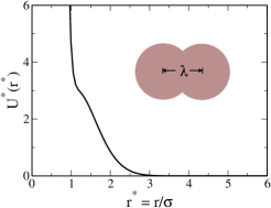
Figure 1: Effective potential versus distance in reduced units.

We performed molecular dynamics simulations in the canonical ensemble using $N=500$ particles (250 dimers) in a cubic box of volume $V$ with periodic boundary conditions in the three directions, interacting with the intermolecular potential described above. The number density of the system is then $\rho=N/V$. The cutoff radius was set to $5.5\sigma$. Pressure, temperature, density, and diffusion are calculated in dimensionless units:

$$T^{*} \equiv \frac{k_{B}T}{\epsilon}\;$$

$$\rho^{*} \equiv \rho\sigma^{3}$$

$$P^{*} \equiv \frac{P\sigma^{3}}{\epsilon}$$

$$D^{*} \equiv \frac{D(m/\epsilon)^{1/2}}{\sigma}\;.$$ (2)

In some state points we also carried out simulations with the same model but with 1000 (500 dimers) and 2000 (1000 dimers) particles using the Large-scale Atomic/Molecular Massively Parallel Simulator (LAMMPS) Plimpton (1995) with essentially the same results. Further simulation details are discussed elsewhere de Oliveira et al. (2006a).

Preliminary simulations showed that depending on the chosen temperature and density the system was in a fluid phase but became metastable with respect to the solid phase. In order to locate the phase boundary between the solid and the fluid phases two sets of simulations were carried out, one beginning with the molecules in a ordered crystal structure and the other beginning with the molecules in a random, liquid, starting structure obtained from previous equilibrium simulations. Thermodynamic and dynamic properties were calculated over 700 000 steps for the first set (and 900 000 steps for the second set), previously equilibrated over 200 000 (or 300 000) steps. The time step was 0.001 in reduced units and the time constant of the Berendsen thermostat Berendsen et al. (1984) was 0.1 in reduced units. The internal bonds between the particles in each dimer remain fixed using the SHAKE Ryckaert et al. (1977) algorithm, with a tolerance of $10^{-12}$.

The stability of the system was checked by analyzing the dependence of pressure on density and also by visual analysis of the final structure, searching for cavitation. The structure of the system was characterized using the intermolecular radial distribution function, $g(r)$ (RDF), which does not take into account the correlation between atoms belonging to the same molecule. The diffusion coefficient was calculated using the slope of the least square fit to the linear part of the mean square displacement, $<r^{2}(t)>$ (MSD), averaged over different time origins.

For analyzing the structure we define the structural anomaly region as the region where the translational order parameter $t$, given by

$$t\equiv\int_{0}^{\xi_{c}}|g(\xi)-1|d\xi,$$ (3)

decreases upon increasing density. Here $\xi\equiv r\rho^{1/3}$ is the distance $r$ in units of the mean interparticle separation $\rho^{-1/3}$, $\xi_{c}$ is the cutoff distance set to half of the simulation box times $\rho^{-1/3}$, as in Ref. de Oliveira et al. (2006b), $g(\xi)$ is the radial distribution function as a function of the (reduced) distance $\xi$ from a reference particle. For an ideal gas $g=1$ and $t=0$. In the crystal phase $g\neq 1$ over long distances and $t$ is large.

III Results

III.1 The phase-diagram

Fig. 2 shows (a) the pressure-temperature phase-diagram, (b) the radial distribution functions, (c) the mean square displacements and, finally, (d) snapshots of the system at some relevant thermodynamic state points. The pressure-temperature phase diagram, illustrated in Fig. 2(a), displays at low temperatures a low density solid phase, a high density solid phase, a low density fluid phase, and a high density fluid phase. Near the boundaries of the high density solid phase, a liquid crystal-like (LCL) phase was also identified, as discussed below.

At intermediate temperatures as the pressure is isothermally increased [following the arrow in the figure 2(a)] the system goes as follows: for low pressures the system is in the fluid phase, then as pressure increases it becomes solid, for higher pressures it becomes fluid again and then liquid crystal for even higher pressures. For very high pressures the system becomes solid and for even more higher pressures it becomes fluid again (not shown in the figure).

The nature of the phases was investigated from three different ways: the radial distribution function, Fig. 2(b), the mean square displacement, Fig. 2(c), and the structural snapshots, Fig. 2(d). While for $P^{*}=1.17$ and $7.24$ Fig. 2(d) shows ordered structures, for $P^{*}=0.194$ and $4.19$ the structure is disordered, what could be typical for a liquid or a glass, depending on the mobility of particles in the system. According to the mean square displacement illustrated in Fig. 2(c), for $P^{*}=0.194$ and $P^{*}=4.19$ particles show high mobility, whereas for $P^{*}=1.17$ particles do not move. This would be already expected from the corresponding radial distribution function shown in Fig. 2(b). However, for $P^{*}=7.24$ particles move almost as fast as in a liquid phase, but the corresponding radial distribution function and structural snapshots are rather solid-like.

Which type of phase could be present in $P^{*}=7.24$? In order to answer this question a movie with the evolution of the configurations was made. This movie (available as supplementary material) shows that in this case particles actually move, but only in a string-like fashion, what characterizes a liquid crystal-like (LCL) phase. Besides the presence of this liquid crystal phase, the dumbbell system also exhibit a fluid phase at very high pressures.

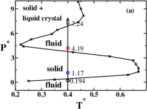
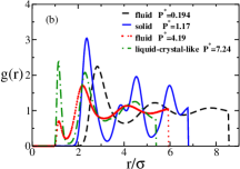
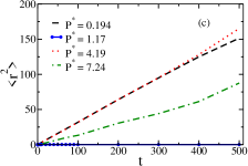
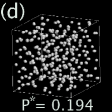
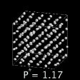
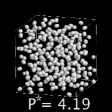
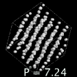
Figure 2: (a) Reduced pressure versus reduced temperature phase-diagram showing the liquid and solid phases. The arrow at $T^{*}=0.4$ crosses the regions with $P^{*}=$ 0.194, 1.17, 4.19, and 7.24 illustrated in the radial distribution function. (b) Radial distribution function versus reduced distance for $T^{*}=0.4$ and $P^{*}=$ 0.194, 1.17, 4.19, and 7.24. (c) Mean square displacement versus time for the four regions illustrated in (a): fluid, solid, fluid, and liquid crystal. With the slope of the MSD versus time for $P^{*}=$0.194, 1.17, 4.19, 7.24 we calculate the diffusion coefficient that is zero for $P^{*}=1.17$. (d) Snapshots of the configurations for $T^{*}=0.4$ and the same pressures as in panel (a).

III.2 The anomalies

Similarly to the monomeric system previously studied de Oliveira et al. (2006a) anomalies were also found in its dumbbells version, considered in this work. We focused in the three anomalies already found in the monomers case, i.e., the density, diffusion, and structural anomalies, as described below.

(i) The density anomaly is the unusual expansion of the system upon cooling at constant pressure, a well-known effect which happens in water as discussed in the Introduction. In NPT-constant ensemble this anomaly is characterized by a maximum of the density along isobars in the density-temperature plane. Through thermodynamic relations Kumar et al. (2006) we are able to equivalently detect this anomaly by searching for a minimum of the pressure along isochores in the pressure-temperature phase-diagram. This was the technique used in this work since it is more suitable for the NVT ensemble.

The density anomaly region for both (a) dimeric and (b) monomeric systems are shown in Fig. 3 as solid bold lines. Both dimeric and monomeric systems have the usual nose-shaped TMD line format, also found in molecular models for water Errington and Debenedetti (2001); Netz et al. (2001) as well as for other isotropic potentials Xu et al. (2006); Yan et al. (2005, 2006); de Oliveira et al. (2008b).

For the dumbbells model the density anomaly region is located at higher pressures and temperatures and occupies a much larger region in the pressure-temperature phase-diagram than that observed for the the monomeric system. This can be evidenced by values for the maximum and minimum pressures and temperatures which enclose the TMD line for both systems, as shown in Table III.2.

(ii) We also studied the molecular mobility calculating the diffusion coefficient using the the mean-square displacement averaged over different initial times,

$$\langle\Delta r(t)^{2}\rangle=\langle[r(t_{0}+t)-r(t_{0})]^{2}\rangle\;.$$ (4)

Then the diffusion coefficient is obtained from the relation

$$D=\lim_{t\to\infty}\langle\Delta r(t)^{2}\rangle/6t\;.$$ (5)

Diffusion anomaly was also found in the dumbbells system. The usual procedure for detecting the dynamic anomaly region is to plot the diffusion coefficient versus density for fixed temperatures de Oliveira et al. (2006a, b); Kumar et al. (2006); Xu et al. (2006); de Oliveira et al. (2008b) as depicted in Fig. 4. From this figure we see that for a certain range of densities the diffusion coefficient anomalously increases under increasing density, changing its slope from negative to positive into this range. This determines a local maxima and minima for the $D(\rho)$ plot. These extrema points can be mapped into a pressure-temperature plane, determining the lines of extrema in the diffusion coefficient inside which particles move faster under compression – or, equivalently, under increasing density.

Fig. 3(a) illustrates the local diffusivity maxima and minima as dashed lines. Comparison between Fig. 3(a) and Fig. 3(b) indicates that the diffusion anomaly region for dumbbells occupies a larger region in the p-T plane than the diffusion anomaly region for the monomeric system. This can be evidenced by values for the maximum and minimum pressures and temperatures which enclose the diffusion anomalous region in Table III.2.

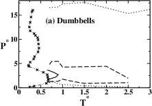
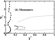
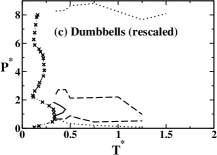
Figure 3: Pressure versus temperature phase diagram for (a) dimeric and (b) monomeric particles interacting through the potential illustrated in Fig. 1, and (c) the rescaled dimeric results, in which pressure and temperature from (a) are divided by 2 (see the text for more details). The results shown in panel (b) were adapted from Refs. de Oliveira et al. (2006a) and de Oliveira et al. (2006b). The reentrant line with crosses in (a) represent the boundary between the fluid and the solid phases. The bold solid, dashed and dotted lines represent the TMD, D extrema, and the region of the structural anomaly respectively, in both (a) and (b) panels.

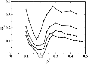
Figure 4: Diffusion coefficient versus density at fixed temperatures, which are $T^{*}=$0.65, 0.75, 0.90, and 1.20 from bottom to top.

(iii) We also study the behavior of the translational order parameter. We see from figure 5 that $t$ decreases for increasing density in a certain range of densities, contrary of what expected for a normal fluid. The local maximum/minimum in the $t(\rho)$ plot can be mapped into a pressure-temperature plane (as discussed above) giving the bounding lines for the region of structural anomaly in the $P$-$T$ phase diagram, i.e., dotted lines in Fig. 3.

Comparison between Fig. 3(a) and Fig. 3(b) shows that the structural anomaly region is much broader for the dumbbells than for the monomers. It shall be stressed that the dumbbells system can be found in the liquid phase at pressures at high as $P^{*}=17.6$, which bounds the upper limit of the structural anomaly region. On the other hand, the lower limit for the structural anomaly region of the dumbbells model achieves pressures as low as 0.14 in reduced units, even lower than for the monomers case (which is 0.32 in reduced units).

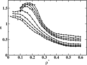
Figure 5: Translational order parameter for the dumbbells system against density for fixed temperatures, which are $T^{*}=$ 0.7, 0.8, 0.9, 1.0, 1.5, 2.0, 2.5, and 3.0 from top to bottom.

Maximum and minimum pressures and temperatures which bound (A) the TMD line (solid in Fig. 3) in both systems, (B) dynamic anomaly region (bounded by dashed lines in Fig. 3) for both systems and (C) the structural anomaly region (bounded by dotted lines in Fig. 3) for both systems. A B C Dimers Monomers Dimers Monomers Dimers Monomers $P^{*}$ max. 3.66 0.90 5.42 0.94 $17.6$ 0.94 $P^{*}$ min. 1.73 0.55 0.90 0.43 $0.14$ 0.43 $T^{*}$ max. 0.90 0.26 2.50 0.40 $>3.0$ 1.00 $T^{*}$ min. 0.65 0.18 0.70 0.18 $<0.70$ 0.25

In principle the differences between the monomeric and the dimeric system could be interpreted by assuming that a dimeric molecule is a monomeric with twice the potential $\epsilon$. In order to test if this would be the case, we rescaled pressure and temperature, $T^{**}=T^{*}/2$ and $P^{**}=P^{*}/2$, and replot the diagram illustrated in Fig. 3 (a) obtaining Fig. 3 (c). Even in this case the dumbbell system shows remarkable differences when compared with the monomeric case.

The addition of anisotropy changes the phase diagram of the fluid phase being the differences significantly larger regarding the regions of the diffusion and structural anomalies. A proper choice of parameters, maybe a fine tuning of the distance $\lambda$ between the two particles of the same dimer, could lead to a specific range in the pressure-temperature phase space of the anomalies.

IV conclusion

In resume, we have addressed the question if just including anisotropy in a core-softened potential would lead to a modification in its anomalies and phases. For that purpose we have investigated a dimeric version of a previously studied monomeric model whose particles were subject to a core-softened potential interaction de Oliveira et al. (2006a, b).

We have found a much richer phase-diagram for the dimers than that one obtained with the monomers. While for the monomeric system the solid phase is at temperatures much lower than the temperatures of the TMD region, for the dumbbell case the solid phase occupies a much wider region in temperatures and terminates at the edge of the TMD region. This indicates that the anisotropy favors certain ordering of the system at low temperatures and low or intermediate pressures. In the case of the dimeric particles two regions of solid phases separated by a liquid crystal region were observed, suggesting that the two length scales together with the anisotropic arrangement result in two solid phase densities. Even more surprising a very high pressure a liquid phase is also observed.

The thermodynamic, dynamic, and structural anomalous regions maintain the same hierarchy in the dimeric case as observed in the monomeric system. The structural anomalous region occupies a wider region in the pressure temperature phase-diagram when compared with the diffusion anomalous region and this region occupies a wider region when compared with the density anomalous region. This hierarchy is also observed in water Netz et al. (2001, 2002b). The dumbbell system, however, has pressures and temperatures in these anomalous regions much larger than the ones observed in the monomeric case. This behavior could be in principle explained mapping the dumbbell in a monomer with twice the potential interaction keeping the same interparticle distance. Since pressure and temperature scale with the interparticle potential, increasing the potential would lead to an increase in pressure and temperature.

In resume, the addition of an anisotropy in a core-softened potential lead to a richer phase-diagram, but does not eliminates the thermodynamic, dynamic, and structural anomalies present in the isotropic system, but enlarges the solid state region. This result indicates that the use of dimers, trimers of even polymers of particles interacting with this isotropic potentials is a promissing way to design complex molecules which might lead to systems with the same anomalies present in water or even other kinds of anomalous behavior.

References

- Krekelberg et al. (2008) W. P. Krekelberg, J. Mittal, V. Ganesan, and M. Truskett, T, Phys. Rev. E 77, 041201 (2008).
- Scala et al. (2000) A. Scala, M. R. Sadr-Lahijany, N. Giovambattista, S. V. Buldyrev, and H. E. Stanley, J. Stat. Phys. 100, 97 (2000).
- Franzese et al. (2001) G. Franzese, G. Malescio, A. Skibinsky, S. V. Buldyrev, and H. E. Stanley, Nature (London) 409, 692 (2001).
- Buldyrev et al. (2002) S. V. Buldyrev, G. Franzese, N. Giovambattista, G. Malescio, M. R. Sadr-Lahijany, A. Scala, A. Skibinsky, and H. E. Stanley, Physica A 304, 23 (2002).
- Buldyrev and Stanley (2003) S. V. Buldyrev and H. E. Stanley, Physica A 330, 124 (2003).
- Skibinsky et al. (2005) A. Skibinsky, S. V. Buldyrev, G. Franzese, G. Malescio, and H. E. Stanley, Phys. Rev. E 69, 061206 (2005).
- Franzese et al. (2002) G. Franzese, G. Malescio, A. Skibinsky, S. V. Buldyrev, and H. E. Stanley, Phys. Rev. E 66, 051206 (2002).
- Balladares and Barbosa (2004) A. Balladares and M. C. Barbosa, J. Phys.: Cond. Matter 16, 8811 (2004).
- de Oliveira and Barbosa (2005) A. B. de Oliveira and M. C. Barbosa, J. Phys.: Cond. Matter 17, 399 (2005).
- Henriques and Barbosa (2005) V. B. Henriques and M. C. Barbosa, Phys. Rev. E 71, 031504 (2005).
- Henriques et al. (2005) V. B. Henriques, N. Guissoni, M. A. Barbosa, M. Thielo, and M. C. Barbosa, Mol. Phys. 103, 3001 (2005).
- Hemmer and Stell (1970) P. C. Hemmer and G. Stell, Phys. Rev. Lett. 24, 1284 (1970).
- Jagla (1998) E. A. Jagla, Phys. Rev. E 58, 1478 (1998).
- Wilding and Magee (2002) N. B. Wilding and J. E. Magee, Phys. Rev. E 66, 031509 (2002).
- Kurita and Tanaka (2004) R. Kurita and H. Tanaka, Science 206, 845 (2004).
- Xu et al. (2005) L. Xu, P. Kumar, S. V. Buldyrev, S.-H. Chen, P. Poole, F. Sciortino, and H. E. Stanley, Proc. Natl. Acad. Sci. U.S.A. 102, 16558 (2005).
- Netz et al. (2004) P. A. Netz, J. F. Raymundi, A. S. Camera, and M. C. Barbosa, Physica A 342, 48 (2004).
- de Oliveira et al. (2006a) A. B. de Oliveira, P. A. Netz, T. Colla, and M. C. Barbosa, J. Chem. Phys. 124, 084505 (2006a).
- de Oliveira et al. (2006b) A. B. de Oliveira, P. A. Netz, T. Colla, and M. C. Barbosa, J. Chem. Phys. 125, 124503 (2006b).
- de Oliveira et al. (2007) A. B. de Oliveira, M. C. Barbosa, and P. A. Netz, Physica A 386, 744 (2007).
- de Oliveira et al. (2008a) A. B. de Oliveira, P. A. Netz, and M. C. Barbosa, Euro. Phys. J. B 64, 481 (2008a).
- de Oliveira et al. (2008b) A. B. de Oliveira, G. Franzese, P. A. Netz, and M. C. Barbosa, J. Chem. Phys 128, 064901 (2008b).
- de Oliveira et al. (2009) A. B. de Oliveira, P. A. Netz, and M. C. Barbosa, Europhys. Lett. 85, 36001 (2009).
- Fomin et al. (2008) D. Y. Fomin, D. Frenkel, N. V. Gribova, and V. N. Ryzhov, J. Chem. Phys. 127 (2008).
- Almarza et al. (2009) N. G. Almarza, J. A. Capitan, J. A. Cuesta, and E. Lomba, J. Chem. Phys 131, 124506 (2009).
- Pretti and Buzano (2004) M. Pretti and C. Buzano, J. Chem. Phys 121, 11856 (2004).
- Gibson and Wilding (2006) H. M. Gibson and N. B. Wilding, Phys. Rev. E 73, 061507 (2006).
- Debenedetti et al. (1996) P. G. Debenedetti, F. Sciortino, and H. E. Stanley, Phys. Rev. E 53, 6144 (1996).
- Mishima and Stanley (1998) O. Mishima and H. E. Stanley, Nature (London) 396, 329 (1998).
- Netz et al. (2001) P. A. Netz, F. W. Starr, H. E. Stanley, and M. C. Barbosa, J. Chem. Phys. 115, 344 (2001).
- Errington and Debenedetti (2001) J. R. Errington and P. D. Debenedetti, Nature (London) 409, 318 (2001).
- Netz et al. (2002a) P. A. Netz, F. W. Starr, M. C. Barbosa, and H. E. Stanley, J. Mol. Phys. 101, 159 (2002a).
- Cho et al. (1996) C. H. Cho, S. Singh, and G. W. Robinson, Faraday Discuss. 103, 19 (1996).
- Egorov (2008a) S. A. Egorov, J. Chem. Phys. 128, 174503 (2008a).
- Egorov (2008b) S. A. Egorov, J. Chem. Phys. 129, 024514 (2008b).
- Zhou (2006) S. Zhou, Phys. Rev. E 74, 031119 (2006).
- Zhou (2008) S. Zhou, Phys. Rev. E 77, 041110 (2008).
- Zhou (2009) S. Zhou, J. Chem. Phys. 130, 054103 (2009).
- Xu et al. (2006) L. Xu, S. Buldyrev, C. A. Angell, and H. E. Stanley, Phys. Rev. E 74, 031108 (2006).
- Yan et al. (2005) Z. Yan, S. V. Buldyrev, N. Giovambattista, and H. E. Stanley, Phys. Rev. Lett. 95, 130604 (2005).
- Yan et al. (2006) Z. Yan, S. V. Buldyrev, N. Giovambattista, P. G. Debenedetti, and H. E. Stanley, Phys. Rev. E 73, 051204 (2006).
- Franzese (2007) G. Franzese, J. Mol. Liq. 136, 267 (2007).
- Thurn and Ruska (1976) H. Thurn and J. Ruska, J. Non-Cryst. Solids 22, 331 (1976).
- Tsuchiya (1991) T. Tsuchiya, J. Phys. Soc. Jpn. 60, 227 (1991).
- Sauer and Borst (1967) G. E. Sauer and L. B. Borst, Science 158, 1567 (1967).
- Kennedy and Wheeler (1983) S. J. Kennedy and J. C. Wheeler, J. Chem. Phys. 78, 1523 (1983).
- Angell et al. (2000) C. A. Angell, R. D. Bressel, M. Hemmatti, E. J. Sare, and J. C. Tucker, Phys. Chem. Chem. Phys. 2, 1559 (2000).
- Sharma et al. (2006) R. Sharma, S. N. Chakraborty, and C. Chakravarty, J. Chem. Phys. 125, 204501 (2006).
- Shell et al. (2002) M. S. Shell, P. G. Debenedetti, and A. Z. Panagiotopoulos, Phys. Rev. E 66, 011202 (2002).
- Poole et al. (1997) P. H. Poole, M. Hemmati, and C. A. Angell, Phys. Rev. Lett. 79, 2281 (1997).
- Sastry and Angell (2003) S. Sastry and C. A. Angell, Nature Mater. 2, 739 (2003).
- Kriebel and Winkelmann (1996) C. Kriebel and J. Winkelmann, J. Chem. Phys. 105, 9316 (1996).
- Vega et al. (2003) C. Vega, C. McBride, E. de Mibuel, B. F. J., and A. Galindo, J. Chem. Phys. 118, 10696 (2003).
- Plimpton (1995) S. J. Plimpton, J. Comp. Phys. 117, 1 (1995).
- Berendsen et al. (1984) H. J. C. Berendsen, J. P. M. Postuma, W. F. van Gunsteren, A. DiNola, and J. R. Haak, J. Chem. Phys. 81, 3684 (1984).
- Ryckaert et al. (1977) J. P. Ryckaert, G. Ciccotti, and H. J. C. Berendsen, J. Comput. Phys. 23, 327 (1977).
- Kumar et al. (2006) P. Kumar, G. Franzese, and H. E. Stanley, Phys. Rev. E 73, 041505 (2006).
- Netz et al. (2002b) P. A. Netz, F. W. Starr, M. C. Barbosa, and H. E. Stanley, Physica A 314, 470 (2002b).