Mesoscopic Shelving Readout of Superconducting Qubits in Circuit QED

Abstract

We present a method for measuring the internal state of a superconducting qubit inside an on-chip microwave resonator. We show that one qubit state can be associated with the generation of an increasingly large cavity coherent field, while the other remains associated with the vacuum. By measuring the outgoing resonator field with conventional devices, an efficient single-shot QND-like qubit readout can be achieved, enabling a high-fidelity measurement in the spirit of the electron-shelving technique for trapped ions. We expect that the proposed ideas can be adapted to different superconducting qubit designs and contribute to the further improvement of qubit readout fidelity.

Superconducting nanocircuits makhlin01 ; qubitpapers are considered promising candidates for diverse implementations of quantum information tasks bouwmeester08 . In this context, circuit quantum electrodynamics (QED) blais04 ; chiorescuwallraff , which studies superconducting qubits makhlin01 ; nakamura99 coupled to on-chip microwave resonators, occupies a central role. To achieve the desired goals, it is important to implement high-fidelity two-qubit gates gatepapers and efficient schemes to read out the qubit state readoutpapers . In both cases, trapped-ion systems represent the state-of-the-art for qubit realizations leibfried03 . In particular, electron-shelving qubit readout has produced fidelity benchmarks of approximately $99.99\%$ ionpapers . These astonishing achievements suggest the potential impact of transferring key ideas from quantum optics to circuit QED. Unfortunately, electron shelving relies strongly on the use of single-photon detectors leibfried03 , which are unavailable in microwave technology in the range $1-10\,\rm{GHz}$ romero08 . Nevertheless, in this manuscript we show that a single-shot QND-like fast qubit readout can be designed by exploiting the electron-shelving concept in circuit QED.

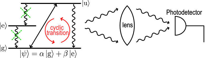
Figure 1: (Color online) Sketch of electron shelving in trapped ions. The $|{\rm g}\rangle\leftrightarrow|{\rm u}\rangle$ transition is driven with a laser beam, performing a cyclic transition and emitting many photons when $|{\rm g}\rangle$ is projected. No photons are detected when $|{\rm e}\rangle$ is measured. Undesired transitions are inhibited via selection rules.

We first present the physics of electron shelving in trapped ions. In Fig. 1, we show a three-level atom where an unknown qubit state $|\psi\rangle=\alpha|{\rm g}\rangle+\beta|{\rm e}\rangle$ is encoded in states $|{\rm g}\rangle$ and $|{\rm e}\rangle$. Via a laser beam, the ground state $|{\rm g}\rangle$ is coupled to a third level $|{\rm u}\rangle$, which can decay producing a continuous cyclic transition. In this case, the qubit is projected onto state $|{\rm g}\rangle$ and many photons are emitted in free space, one at each cycle. In contrast, when the qubit is projected onto state $|{\rm e}\rangle$, no photons are emitted. A lens is used to collect the photons more efficiently by improving the solid angle. Although the photodetector has a low efficiency $\eta_{\rm d}$, the qubit readout fidelity can be very high. Typically, it is estimated through $F=1-e^{-\eta_{\rm d}N}$, which rapidly approaches unity for $\eta_{\rm d}N\gg 1$, $N$ being the number of detected photons. Key elements for electron shelving are the use of three-level qubits, cyclic transitions, selection rules, and photodetectors.

In the following, we present a method for implementing a single-shot QND-like fast high-fidelity readout of superconducting qubits. It preserves the spirit of electron shelving, but it is suitably adapted to existent microwave technology in circuit QED where, for example, single-photon detectors are unavailable. We assume that the qubit is prepared in an unknown pure state and that our task is to measure the spin operator $\sigma^{z}$. We consider a three-level superconducting qubit paspalakis04 ; nori05 inside an on-chip microwave resonator (acting as a cavity), as shown in Fig. 2. The initial qubit state is encoded in the two lower energy levels, $|\psi(0)\rangle=\alpha|{\rm g}\rangle+\beta|{\rm e}\rangle$. In addition, we consider an anharmonic three-level qubit where the transition frequencies are different, $\omega_{\rm ge}\neq\omega_{\rm eu}$. Levels $|{\rm e}\rangle$ and $|{\rm u}\rangle$ are coupled resonantly to a resonator mode, but there is no dynamics because the resonator is initially empty and level $|{\rm u}\rangle$ unpopulated. To start with the readout process, we drive the transition between levels $|{\rm e}\rangle$ and $|{\rm u}\rangle$ with a coherent resonant field with angular frequency $\omega_{\rm d}$ and amplitude $\mu$ transversal to the resonator axis.

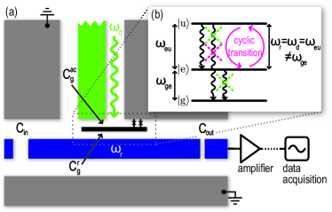
Figure 2: (Color online) Sketch of the mesoscopic shelving qubit readout. (a) A three-level superconducting qubit is capacitively coupled ($C_{\rm g}^{\rm r}$) to a coplanar wave-guide microwave resonator with angular frequency $\omega_{\rm r}$ and input and output capacitors $C_{\rm in}$ and $C_{\rm out}$, respectively. The qubit is also coupled to an orthogonal transmission line via $C_{\rm g}^{\rm ac}$. (b) The transition $\omega_{\rm eu}$ is resonant to the cavity and is driven with a transversal coherent field (magenta line). Transition rates $|{\rm e}\rangle\rightarrow|{\rm g}\rangle$ and $|{\rm u}\rangle\rightarrow|{\rm g}\rangle$ are reduced by Purcell effect (green dashed lines) or selection rules (magenta dashed lines).

The system Hamiltonian, in the energy eigenbasis and after a rotating-wave approximation, can be written as

$$H = \frac{\hbar\omega_{\rm eu}}{2}\sigma^{z}_{\rm eu}+\hbar\omega_{\rm r}a^{\dagger}a+\hbar g_{\rm eu}\left(\sigma_{\rm eu}^{+}a+\sigma_{\rm eu}^{-}a^{\dagger}\right)$$ (1)

$$+\hbar\Omega_{\rm eu}\left(\sigma_{\rm eu}^{+}e^{-i\omega_{\rm d}t}+\sigma_{\rm eu}^{-}e^{i\omega_{\rm d}t}\right)$$

$$+\hbar\lambda\left(a^{\dagger}e^{-i\omega_{\rm d}t}+ae^{i\omega_{\rm d}t}\right).$$

Here, $\sigma^{z}_{\rm eu}\equiv|{\rm u}\rangle\langle{\rm u}|-|{\rm e}\rangle\langle{\rm e}|$, $\sigma^{+}_{\rm eu}\equiv|{\rm u}\rangle\langle{\rm e}|$, $\sigma^{-}_{\rm eu}\equiv|{\rm e}\rangle\langle{\rm u}|$, $a\>(a^{\dagger})$ are the bosonic annihilation (creation) operators of the resonator field, and $g_{\rm eu}$, $\Omega_{\rm eu}$, and $\lambda$ are coupling strengths. $\lambda$ describes the crosstalk between the driving field and the resonator, and its origin typically depends on the specific setup mariantoni08 . The qubit readout happens under the resonant condition $\omega_{\rm r}=\omega_{\rm d}=\omega_{\rm eu}$. We assume that the transition $|{\rm u}\rangle\rightarrow|{\rm e}\rangle$ is sufficiently long-lived such that it does not decay during the short operation time. Finally, our model considers enough energy anharmonicity so that the radiative decay rates associated with the transitions $|{\rm e}\rangle\rightarrow|{\rm g}\rangle$ and $|{\rm u}\rangle\rightarrow|{\rm g}\rangle$ are reduced by Purcell effect. Also, these transitions can be reduced exploiting the characteristic selection rules and symmetry breaking properties of superconducting qubits nori05 ; deppe08 .

We rewrite the Hamiltonian in a reference frame rotating with the driving field frequency via the transformation $U^{\rm rot}=\exp\left[-i\omega_{\rm d}(a^{\dagger}a+\sigma_{\rm eu}^{+}\sigma_{\rm eu}^{-})t\right]$, obtaining

$$H^{\rm rot}\!=\hbar\Omega_{\rm eu}\sigma_{\rm eu}^{x}\!+\!\hbar g_{\rm eu}\left(\sigma_{\rm eu}^{+}a+\sigma_{\rm eu}^{-}a^{\dagger}\right)\!+\!\hbar\lambda\left(a^{\dagger}+a\right),$$ (2)

with $\sigma_{\rm eu}^{x}=\sigma_{\rm eu}^{+}+\sigma_{\rm eu}^{-}$. We now apply the transformation $U^{I}=\exp\left[-i\Omega_{\rm eu}\sigma_{\rm eu}^{x}t\right]$ under the strong-driving condition $\Omega_{\rm eu}\gg g_{\rm eu}$ solano03 , and derive the effective Hamiltonian

$$H_{\rm eff}=\frac{\hbar g_{\rm eu}}{2}(\sigma_{\rm eu}^{+}+\sigma_{\rm eu}^{-})(a+a^{\dagger})+\hbar\lambda\left(a^{\dagger}+a\right)\,.$$ (3)

The first part of the Hamiltonian simultaneously realizes Jaynes-Cummings and anti-Jaynes-Cummings resonant interactions. It does not generate Rabi oscillations, but conditional field displacements solano03 , while the second term implements a resonant displacement. The initial qubit–field state is $|\psi(0)\rangle=\alpha|\,{\rm g}\,\rangle|0\rangle+\beta\left(|+\rangle+|-\rangle\right)|0\rangle/\sqrt{2}$, with $\sigma_{\rm eu}^{x}|\pm\rangle=\pm|\pm\rangle$. After an interaction time $t$, the state is

$$|\psi(t)\rangle = \alpha|{\rm g}\rangle|\bar{\nu}(t)\rangle+\frac{\beta}{\sqrt{2}}\big{[}|+\rangle|\bar{\eta}(t)+\bar{\nu}(t)\rangle$$ (4)

$$\qquad\qquad\qquad+|-\rangle|-\bar{\eta}(t)+\bar{\nu}(t)\rangle\big{]}.$$

Here, the coherent states $|\,\pm\bar{\eta}(t)+\bar{\nu}(t)\rangle$, with $\bar{\eta}(t)=-ig_{\rm eu}t/2$ and $\bar{\nu}(t)=-i\lambda t$, are generated by the displacement operators $\mathcal{D}[\pm\bar{\eta}(t)+\bar{\nu}(t)]=\exp\left([\pm\bar{\eta}(t)+\bar{\nu}(t)]a^{\dagger}-[\pm{\bar{\eta}}^{\ast}(t)+{\bar{\nu}}^{\ast}(t)]a\right)$. In general, we expect the crosstalk to be small, so that $\lambda\ll g_{\rm eu}/2$ and $\bar{\nu}(t)\ll\bar{\eta}(t)$. When the measurement starts, the applied driving field yields many intracavity photons ${\bar{N}}^{\rm e}_{\rm in}(t)\approx|\bar{\eta}(t)|^{2}$ with probability $|\alpha|^{2}$ if the state $|{\rm e}\rangle$ is projected. If the state $|{\rm g}\rangle$ is selected, it yields a few photons ${\bar{N}}^{\rm g}_{\rm in}(t)=|\bar{\nu}(t)|^{2}\ll|\bar{\eta}(t)|^{2}$ with probability $|\beta|^{2}$.

We now add to our model a zero-temperature dissipative reservoir for the cavity field, characterized by a decay rate $\kappa$. The corresponding master equation reads

$$\dot{\rho}_{\rm q-f}=-\frac{i}{\hbar}[H_{\rm eff},\rho_{\rm q-f}]+\mathcal{L}_{\rm f}\,\rho_{\rm q-f}\ \ ,$$ (5)

with $\mathcal{L}_{\rm f}\rho_{\rm q-f}\equiv\kappa L[a]\rho_{\rm q-f}$ such that

$$\mathcal{L}_{\rm f}\rho_{\rm q-f}=\kappa\left(2a\rho_{\rm q-f}a^{\dagger}-a^{\dagger}a\rho_{\rm q-f}-\rho_{\rm q-f}a^{\dagger}a\right)/2$$ (6)

and expansion $\rho_{\rm q-f}(t)=\sum_{j,k={\rm g},-,+}|j\rangle\langle k|\otimes\rho^{jk}_{\rm f}(t)$. Here, it is possible to find analytical solutions for $\rho^{jk}_{\rm f}(t)=\langle j|\rho_{\rm q-f}(t)|k\rangle$ using standard phase-space tools lougovski and the method of characteristics to solve the partial differential equations barnett . The solutions read

$$\rho^{++}_{\rm f}(t) = \frac{|\beta|^{2}}{2}|\eta(t)+\nu(t)\rangle\langle\eta(t)+\nu(t)|,$$

$$\rho^{--}_{\rm f}(t) = \frac{|\beta|^{2}}{2}|-\eta(t)+\nu(t)\rangle\langle-\eta(t)+\nu(t)|,$$

$$\rho^{{\rm gg}}_{\rm f}(t) = |\alpha|^{2}|\nu(t)\rangle\langle\nu(t)|,$$

$$\rho^{+-}_{\rm f}(t) = \frac{|\beta|^{2}}{2}\frac{f_{1}(t)}{e^{-2|\eta(t)|^{2}}}|\eta(t)+\nu(t)\rangle\langle-\eta(t)+\nu(t)|,$$

$$\rho^{{\rm g}+}_{\rm f}(t) = \frac{\beta^{\ast}\alpha}{\sqrt{2}}\frac{f_{2}(t)}{e^{-|\eta(t)|^{2}/2}}|\nu(t)\rangle\langle\eta(t)+\nu(t)|,$$

$$\rho^{{\rm g}-}_{\rm f}(t) = \frac{\beta^{\ast}\alpha}{\sqrt{2}}\frac{f_{2}(t)}{e^{-|\eta(t)|^{2}/2}}|\nu(t)\rangle\langle-\eta(t)+\nu(t)|,$$ (7)

where

$$f_{1}(t) = \exp\left(-2\frac{g_{\rm eu}^{2}}{\kappa}t+\frac{4g_{\rm eu}^{2}}{\kappa^{2}}\left[1-e^{-\kappa t/2}\right]\right),$$

$$f_{2}(t) = \exp\left(-\frac{g_{\rm eu}^{2}}{2\kappa}t+\frac{g_{\rm eu}^{2}}{\kappa^{2}}\left[1-e^{-\kappa t/2}\right]\right),$$ (8)

with $\eta(t)=-ig_{\rm eu}/\kappa\left[1-e^{-\kappa t/2}\right]$, $\nu(t)=-2i\lambda/\kappa\left[1-e^{-\kappa t/2}\right]$. For a small crosstalk $\lambda$, the leakage rate of outgoing photons $N^{\rm e}_{\rm out}(t)$ when state $|{\rm e}\rangle$ is measured can be estimated as

$$N^{\rm e}_{\rm out}(t)=\kappa\,N^{\rm e}_{\rm in}(t)=\kappa\,|\eta(t)|^{2}=\frac{g_{\rm eu}^{2}}{\kappa}\left(1-e^{-\kappa t/2}\right)^{2},$$ (9)

where $N^{\rm e}_{\rm in}(t)=|\eta(t)|^{2}$ is the intracavity mean photon number. $N^{\rm e}_{\rm out}(t)$ grows very fast well below decoherence times. It can be measured, e.g., by means of a data acquisition card, which follows a phase-preserving or even a more quiet phase-sensitive phase:sensitive:amps linear amplifier. We also notice that one can profit from the generated large intracavity field to adapt to other readout techniques hofheinz08 .

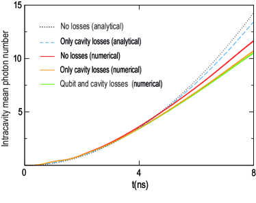
Figure 3: (Color online) Intracavity mean photon number for the mesoscopic shelving readout of a CPB in the charge-phase regime with conservative parameter set: $E_{\rm C}/\hbar=E_{\rm J}/\hbar=2\pi\times 10\,\rm{GHz}$, $g_{\rm eu}=\Omega_{\rm eu}/5=2\pi\times 150\,\rm{MHz}$, $\kappa=2\pi\times 1.6\,\rm{MHz}$, $\gamma_{\rm eu}=10\gamma_{\rm ge}=2\,\rm{MHz}$, $\gamma_{\rm gu}=0$, and $\gamma_{\varphi}=2\,\rm{MHz}$. The dotted and dashed curves correspond to the analytical results and the solid lines to the numerical results. Note that, in the absence of losses, there is still a difference between the analytical and the numerical results. This is due to the off-resonant couplings and multilevel character of the realistic model.

The physical concepts behind the mesoscopic shelving are general and can be adapted to different qubits and setups. We exemplify here with a possible adaptation to a Cooper-pair box (CPB) coupled to a microwave resonator of angular frequency $\omega_{\rm r}$. Here, the CPB has a Josephson energy $E_{\rm J}$ and charging energy $E_{\rm C}=(2e)^{2}/2C_{\rm tot}$, where $C_{\rm tot}$ is the total island capacitance. We refer to a system that is essentially the one in Ref. blais04 , with the addition of a transmission line, orthogonal to the resonator, for driving the qubit (see Fig. 2). Using $n$, the number operator for excess Cooper pairs on the CPB island, and $\varphi$, the phase difference across the Josephson junction, the Hamiltonian can be written as

$$H = E_{\rm C}(n-n_{x})^{2}-E_{\rm J}\cos{\varphi}+\hbar\omega_{\rm r}a^{\dagger}a\ ,$$ (10)

where

$$(2e)n_{x} \!\!=\!\! C^{\rm dc}_{\rm g}V^{\rm dc}_{\rm g}+C^{\rm ac}_{\rm g}V^{\rm ac}_{\rm g}(t)+C^{\rm r}_{\rm g}V_{0}(a^{\dagger}+a)\,.$$ (11)

Here, $C^{l}_{\rm g}$ ($l=\{{\rm dc,ac,r}\}$) are effective gate capacitances, $V_{\rm g}^{\rm dc}$ is the gate voltage that defines the working point (we choose the so-called “sweet spot” $C^{\rm dc}_{\rm g}V_{\rm g}^{\rm dc}/2e=1/2$), $V_{\rm g}^{\rm ac}$ is the voltage of the orthogonal driving field, $a$ ($a^{\dagger}$) refers to the cavity field, and $V_{0}$ is the resonator zero-point voltage. Note that the CPB is coupled to the resonator and the ac drive via the charge number operator. The classical gate charge $C_{\rm g}^{\rm ac}V_{\rm g}^{\rm ac}$ and the quantum gate charge $C_{\rm g}^{\rm r}V_{0}$ represent small deviations from the sweet spot.

We can rewrite $H$ in a basis of CPB eigenstates restricted to the first three energy levels, the ground state $|{\rm g}\rangle$ and the first and second excited states, $|{\rm e}\rangle$ and $|{\rm u}\rangle$, respectively. This leads to an effective Hamiltonian for the driven qubit–resonator system,

$${\cal H} = {\cal H}_{0}+{\cal H}_{\rm int}+{\cal H}_{\rm d}\ ,$$ (12)

$${\cal H}_{0} = \sum_{j={\rm g,e,u}}E_{j}|j\rangle\langle j|+\hbar\omega_{\rm r}a^{\dagger}a\ ,$$

$${\cal H}_{\rm int} = \hbar(g_{\rm gu}|{\rm u}\rangle\langle{\rm g}|+g_{\rm eu}|{\rm u}\rangle\langle{\rm e}|)(a^{\dagger}+a)\,+\,{\rm H.c.}\ ,$$

$${\cal H}_{\rm d} = (\cos{\omega_{\rm d}t})\sum_{j<k={\rm g,e,u}}(\hbar\Omega_{jk}|j\rangle\!\langle k|\,+\,{\rm H.c.})\ .$$

The coupling strengths $g_{jk}\equiv(E_{\rm C}/\hbar e)n_{jk}C_{\rm g}^{\rm r}V_{0}$ and $\Omega_{jk}\equiv(E_{\rm C}/\hbar e)n_{jk}C_{\rm g}^{\rm ac}V^{\rm ac}_{\rm g}(t)$ are proportional to the matrix elements $n_{jk}=\langle k|n|j\rangle$. In order to obtain the time evolution of the complete system, including the relaxation and dephasing of qubit transitions, we numerically solve the master equation for the qubit-resonator density matrix $\rho(t)$

$$\dot{\rho} = -\frac{i}{\hbar}[{\cal H},\rho]+{\mathcal{L}}_{\rm f}\rho+{\mathcal{L}}_{\rm q}\rho\ ,$$ (13)

where, using the functional $L$ defined in Eq. (5), we have

$${\mathcal{L}}_{\rm q}\rho \!\!=\!\! \sum_{j<k}\gamma_{jk}L\big{[}\,|k\rangle\langle j|\,\big{]}\rho+\sum_{j}\frac{\gamma_{\varphi}}{2}L\big{[}\,|j\rangle\langle j|\,\big{]}\rho\,.$$ (14)

Here, $\kappa$ is the decay rate of the resonator, $\gamma_{jk}$ $(j,k=\{{\rm g,e,u}\})$ are the relaxation rates for the transitions $|{\rm e}\rangle\rightarrow|{\rm u}\rangle$ and $|{\rm u}\rangle\rightarrow|{\rm g}\rangle$, and $\gamma_{\varphi}$ is the dephasing rate, which we take to be equal for all coherences. In the numerical solution of Eq. (13), we truncate the resonator Hilbert space to $25$ photon number states due to technical limitations. In addition, we make sure that the population of the fourth qubit eigenstate is negligible. Clearly, the condition $\gamma_{\rm eu}+\gamma_{\rm gu}\ll g_{\rm eu}$ is crucial for our method to be efficient. Therefore, a qubit layout with suppressed $\gamma_{\rm gu}$ is preferred for the shelving readout.

The results for the intracavity mean photon number with a conservative set of parameters, in the analytical and numerical cases, are shown in Fig. 3. We see that, although the full dynamics in Eq. (13) is considerably more complex than the one in Eq. (5), the simple analytical model captures the essence of the system dynamics. The main influence of a realistic description is a small reduction in the intracavity mean photon number. We observe that, given the short interaction times displayed in Fig. 3, the resonator decay rate $\kappa$ alone has a small effect in the cavity population, while the finite lifetime of states $|{\rm e}\rangle$ and $|{\rm u}\rangle$ is slightly more important. In this manner, we feel comfortable to extrapolate the analytical results for the cavity population including cavity losses for short measurement times to make further estimations.

The signal-to-noise ratio (SNR) after a measurement time $\tau_{\rm m}$ is the ratio between the accumulated number of outgoing photons and the accumulated noise blais04 . The latter is dominated by the amplifier noise, $n_{\rm amp}=k_{\rm B}T_{\rm n}/\hbar\omega_{\rm r}\simeq 25$, where $T_{\rm n}$ is its associated noise temperature. In this manner,

$$\mathrm{SNR}(\tau_{\rm m})=\frac{\int_{0}^{\tau_{\rm m}}\kappa N_{\rm in}^{\rm e}(t)dt}{n_{\rm amp}B\tau_{\rm m}}$$ (15)

where $B\equiv\max{\{\kappa,\gamma_{jk}\}}$ is the measurement bandwidth. We now estimate the SNR for three relevant consecutive times. First, we use the maximum simulated time $\tau^{\rm sim}_{\rm m}\simeq 8\,\rm{ns}$, corresponding to $10$ intracavity photons (cf. Fig. 3). We obtain a ${\rm SNR}\simeq 0.2$. Considering that our simulations include all relevant system details without any approximation boissonneault , this is a remarkable result for such an extremely short measurement time. Using our analytical results including resonator dissipation, see Eq. (9), we estimate that a critical measurement time $\tau^{\rm crit}_{\rm m}\simeq 19$ ns is necessary to reach the condition ${\rm SNR}\sim 1$. This is the minimum time required for a single-shot measurement of the qubit state $|{\rm e}\rangle$. Finally, to achieve high-fidelity qubit readout, we choose the measurement time $\tau^{\rm hf}_{\rm m}\simeq 50$ ns which corresponds to ${\rm SNR}\simeq 6.2$ and fidelity $F=1-e^{\rm-SNR}=0.998$. Notably, $\tau^{\rm hf}_{\rm m}\ll 1/\gamma_{\rm ge}$. Consequently, we expect a single-shot measurement of the qubit state $|{\rm e}\rangle$ with fidelities close to $1$. The proposed mesoscopic shelving qubit readout is of a QND-like character, due to the continuous cavity field amplification in each measurement event. In addition, $\tau^{\rm hf}_{\rm m}$ is at least one order of magnitude shorter than typical measurement times employed in the state-of-the-art experiments based on dispersive readouts. Note that, even for a driving-resonator crosstalk of $\lambda=2\pi\times 10\,\rm{MHz}$ mariantoni08 , the cavity population associated with the measurement of state $|{\rm g}\rangle$ is well below the amplifier background noise level.

In summary, we have presented a novel qubit readout scheme based on a mesoscopic shelving technique, allowing a fast high-fidelity single-shot QND-like measurement of superconducting qubits in circuit QED.

We acknowledge stimulating discussions with P. Bertet, M. Hofheinz, A. Wallraff, J. M. Martinis, R. Schoelkopf, R. Bianchetti, and F. Deppe. This work is funded by Deutsche Forschungsgemeinschaft through SFB 631, Heisenberg Programme, German Academic Exchange Service, and German Excellence Initiative via the Nanosystems Initiative Munich (NIM). E.S. thanks Ikerbasque Foundation, UPV-EHU Grant GIU07/40, and EuroSQIP European project.

References

(1)
Y. Makhlin, G. Schön, and A. Shnirman, Rev. Mod. Phys. 73, 357 (2001).
(2)
J.Q. You and F. Nori, Physics Today 58, 42–47 (2005);
J. Clarke and F.K. Wilhelm, Nature 453, 1031 (2008).
(3)
D. Bouwmeester, A. Ekert, A. Zeilinger, The Physics of Quantum Information (Springer Verlag, Berlin, 2008).
(4)
A. Blais, R.-S. Huang, A. Wallraff, S. M. Girvin, and R. J. Schoelkopf, Phys. Rev. A 69, 062320 (2004).
(5)
I. Chiorescu et al., Nature 431, 159 (2004);
A. Wallraff et al., Nature 431, 162 (2004).
(6)
Y. Nakamura, Yu. Pashkin, and J.S. Tsai, Nature 398, 786 (1999).
(7)
T. Yamamoto, Yu.A. Pashkin, O. Astafiev, Y. Nakamura, and J.S. Tsai, Nature 425, 941 (2003);
R. McDermott et al., Science 307, 1299 (2005);
J.H. Plantenberg, P.C. de Groot, C.J.P.M. Harmans, J. E. Mooij, Nature 447, 836 (2007).
(8)
I. Siddiqi et al., Phys. Rev. Lett 93, 207002 (2004);
A. Wallraff et al., Phys. Rev. Lett. 95, 060501 (2005);
M. Steffen et al., Phys. Rev. Lett. 97, 050502 (2006);
A. Lupascu et al., Nature Physics 3, 119 (2007).
(9)
D. Leibfried, R. Blatt, C. Monroe, and D. Wineland, Rev. Mod. Phys. 75, 281 (2003).
(10)
D.B. Hume, T. Rosenband, and D.J. Wineland, Phys. Rev. Lett. 99, 120502 (2007);
A.H. Myerson et al., Phys. Rev. Lett. 100, 200502 (2008).
(11)
G. Romero, J.J. García-Ripoll, and E. Solano, arXiv:0811.3909, accepted in Phys. Rev. Letters.
(12)
J. Siewert and T. Brandes, Adv. Solid State Phys. 44, 181 (2004);
E. Paspalakis and N.J. Kylstra, J. Mod. Optics 51, 1979 (2004);
J. Siewert, T. Brandes, and G. Falci, Opt. Comm. 264, 435 (2006).
(13)
Yu-Xi Liu, J.Q. You, L.F. Wei, C.P. Sun, and F. Nori, Phys. Rev. Lett. 95, 087001 (2005).
(14)
M. Mariantoni et al., Phys. Rev. B 78, 104508 (2008).
(15)
F. Deppe et al., Nature Physics 4, 692 (2008).
(16)
F. Helmer et al., Europhys. Lett. 85, 50007 (2009).
(17)
E. Solano, G.S. Agarwal, and H. Walther, Phys. Rev. Lett.
90, 027903 (2003).
(18)
M. A. Castellanos-Beltran, K. D. Irwin, G. C. Hilton, L. R. Vale,
and K. W. Lehnert, Nature Physics 4, 929 (2008); T. Yamamoto
et al., Appl. Phys. Lett. 93, 042510 (2008).
(19)
M. Hofheinz et al., Nature 454, 310 (2008).
(20)
P. Lougovski, F. Casagrande, A. Lulli, and E. Solano, Phys. Rev. A 76, 033802 (2007).
(21)
S.M. Barnett and P.M. Radmore, Methods in Theoretical Quantum Optics (Oxford University Press, New York, 1997).
(22)
M. Boissonneault, J. M. Gambetta, and A. Blais, Phys. Rev. A 77, 060305 (2008).