Comment on ‘Distorted perovskite with $e_{g}^{1}$ configuration as a frustrated spin system’

Abstract

Interesting magnetic structure found experimentally in a series of manganites RMnO₃, where R is a rare earth, was explained, ostensibly, by Kimura et al, in terms of a classical Heisenberg model with an assumed set of exchange parameters, nearest-neighbor and next-nearest-neighbor interactions, $J_{n}$. They calculated a phase diagram as a function of these parameters for the ground state, in which the important “up-up-down-down” or E-phase occurs for finite ratios of the $J_{n}$. In this Comment we show that this state does not occur for such ratios; the error is traced to an incorrect method for minimizing the energy. The correct phase diagram is given. We also point out that the finite temperature phase diagram presented there is incorrect.

Interesting magnetic phases that had been observed in a series of manganites RMnO₃, with R=holmium in particular, were explained in the cited paper kimura on the basis of a Heisenberg Hamiltonian with classical spins on a 2-d rectangular lattice with ferromagnetic nearest-neighbor exchange parameter, $J_{1}$, and two different antiferromagnetic next-nearest- neighbor parameters, $J_{2}$ and $J_{3}$. (The difference is due to the asymmetric positions of the oxygens resulting from Jahn-Teller distortion). By considering a small set of states including the unusual E-type, or “up-up-down-down” state, they obtained a phase diagram for the ground state, and at finite temperature T. We show that the ground state phase diagram is incorrect, and point out that the finite-T case is also incorrect, the correct results differing qualitatively from those presented there. The importance of these conclusions is heightened by the fact that detailed results of the model calculation are accepted in dong .

Circa 1960 it was shown that guessing various spin states (“reasonable”, or experimentally determined) as ground states of the classical Heisenberg energy,

$$H=\sum J_{ij}\mathbf{S}_{i}\cdot\mathbf{S}_{j},\mbox{where}\ \mathbf{S}_{i}^{2}=1,$$ (1)

with some assumed set of exchange parameters $J_{ij}$, and comparing their energies to arrive at a phase diagram, is fraught with danger, often giving incorrect results. (The spin lengths have been absorbed into the $J^{\prime}s$.) Furthermore, for spins on a Bravais lattice, it was shown lyons1 that the ground state energy is always attained by a simple spiral with the wave vector $\mathbf{Q}$ that minimizes $J(\mathbf{q})$, the Fourier transform of of the exchange parameters $J_{ij}$ (the LK theorem). The energy per spin of a spiral with wave vector $\mathbf{q}$ is just $J(\mathbf{q})$. The spiral concept was introduced in 1959. yoshimori ; kaplan1 ; villain This is relevant to the case discussed in kimura , the lattice considered being a Bravais lattice (one spin per primitive unit cell). The proof of the theorem was via the Luttinger-Tisza method luttinger1 ; luttinger2 ; luttinger3 ; please see the recent review kaplan2 .

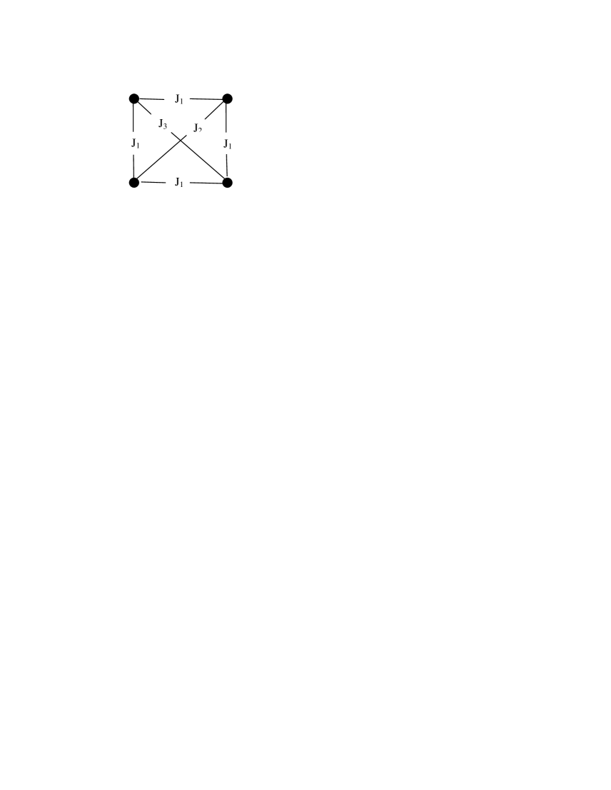
Figure 1: Unit cell showing the exchange interactions between the Mn ions.

The case under consideration kimura essentially involves spins on a square lattice, the 4 n.n. interactions being equal ($J_{1}$), but, due to the internal oxygen structure, the n.n.n interactions $J_{2},J_{3}$ are different. The unit cell is shown in Fig. 1, where the $J^{\prime}s$ are indicated (the oxygens are not shown). Taking the x and y axes respectively, pointing to the right and up with respect to the figure, one readily finds

$$J(\mathbf{q})/2=J_{1}(\cos q_{x}+\cos q_{y})+J_{2}\cos(q_{x}+q_{y})+J_{3}\cos(q_{x}-q_{y}).$$ (2)

In kimura , $J_{1}=-|J_{1}|$ (ferromagnetic n.n. interactions), $J_{2}>0$ and $J_{3}$ is neglected, so that

$$J(\mathbf{q})/(2|J_{1}|)=-(\cos q_{x}+\cos q_{y})+\gamma\cos(q_{x}+q_{y}),$$ (3)

where $\gamma=J_{2}/|J_{1}|$. We first consider $\mathbf{q}$ in the (1,1) direction, $\mathbf{q}=p(\hat{x}+\hat{y})$, so, putting $|J_{1}|=1$,

$$J(\mathbf{q})/2=-2\cos p+\gamma\cos(2p).$$ (4)

The stationary points of this are given by $\sin p=0$ and

$$\cos p=1/(2\gamma)\equiv\cos p_{0};$$ (5)

the latter occurs only if $2\gamma\geq 1$ (the wave vector is real.) The energies at $\mathbf{q}=0$ and at $p_{0}(\hat{x}+\hat{y})\equiv\mathbf{Q}$ are, from (4) and (6),

$$J(0)/2 = -2+\gamma$$

$$J(\mathbf{Q})/2 = -\frac{1}{\gamma}+\gamma(\frac{1}{2\gamma^{2}}-1)=-\frac{1}{2\gamma}-\gamma.$$ (6)

These are equal at $\gamma=1/2$ and in fact

$$J(0)/2-J(\mathbf{Q})/2=2(\gamma+\frac{1}{4\gamma}-1)=\frac{1}{2\gamma}(2\gamma-1)^{2};$$ (7)

that is, the spiral (see the LK theorem) goes below the ferromagnetic state as $\gamma$ increases past 1/2. This contradicts the story in kimura where the ferromagnetic state is indicated to be the ground state all the way to $\gamma=1$. Furthermore, the ground state is not the ‘up-up-down-down” configuration when the ferromagnetic state is first destabilized, as claimed in kimura , but rather a spiral whose wave vector increases continuously from zero at $\gamma=1/2$. Interestingly, as $\gamma\rightarrow\infty,p_{0}\rightarrow\pi/2$, which gives the spiral with a 90^∘ turn angle; and as pointed out in dong , this is degenerate with the “up-up-down-down” state. These results are summarized in Fig. 2.

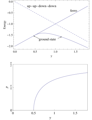
Figure 2: upper: Energy of the ground and other states. lower: Component $p_{0}$ of the spiral wave vector.

To complete the solution to the ground state of this model, we need to check that the lowest $J(\mathbf{q})$ that we found (under the restriction $\mathbf{q}$ in the (1,1) direction), is lowest over all $\mathbf{q}$ in the Brillouin zone. We did this for two values of $\gamma$, namely, 0.4 and 0.6 (sample values in the ferromagnetic region and the spiral region, respectively). Indeed the (1,1) solution is the minimum over all $\mathbf{q}$. We consider this sufficient, although it is easy to check further values of $\gamma$. Lest one might think that we have merely found the lowest spiral (the ferromagnet is the $\mathbf{q}=0$ spiral), and hence ask whether there are other lower-energy states with more than one wave vector (and its negative) in their Fourier representation, we note that because of the place of the calculation in the framework of the Lutttinger-Tisza method and the LK theorem, the conclusion is far stronger: there is no state with a lower energy than the solution given. konstantinidis The finite-T phase diagram in kimura , obtained within the mean-field approximation, shows very complex behavior, numerous long-range-ordered phases (the “Devil’s flower”). However, it was shown by Lyons lyons2 , that for a Bravais lattice with T-independent exchange parameters (the case considered in kimura ), the phase boundary is vertical: a spiral at the ordering temperature remains a spiral with the same wave vector for all T. That is, all the sweet complexity shown in the phase diagram of kimura is not a property of their assumed Hamiltonian.

Thus the question remains, what is the source of the E- or “up-up-down-down” phase found in HoMnO₃? It seems to us that the answer should be found in the standard fundamental model of localized electrons in this insulator, as set forth by P.W. Anderson anderson , and characterized qualitatively for the Heisenberg interactions that are a consequence anderson by the Goodenough-Kanamori rules (seeanderson ). That will include Heisenberg terms with more general interactions than assumed so far, as well as anisotropic terms and isotropic higher-spin terms, e.g. $(\mathbf{S}_{1}\cdot\mathbf{S}_{2})^{2}$, etc. One important aspect of anisotropy is that it can remove the degeneracy of the 90^∘ spiral and the E-state (this observation renders incorrect the argument in dong leading to their conclusion that the “classical spin model is not suitable to explore in a single framework the many phases found in RMnO₃ manganites”).

References

- (1) T. Kimura, S. Ishihara, H. Shintani, T. Arima, K. T. Takahashi, K. Ishizaka, and Y. Tokura, Phys. Rev. B 68, 060403(R) (2003).
- (2) S. Dong, R. Yu, S. Yunoki, J.-M. Liu, and E. Dagotto, Phys. Rev. B 78, 155121 (2008).
- (3) D. H. Lyons and T. A. Kaplan, Phys. Rev. B 120, 1580 (1960)
- (4) A. Yoshimori, J. Phys. Soc. Japan 14 807 (1959).
- (5) T. A. Kaplan, Phys. Rev. 116 888 (1959).
- (6) J. Villain, J. Phys. Chem. Solids 11 303 (1959).
- (7) J. M. Luttinger, Phys. Rev. 81 1015 (1951).
- (8) J. M. Luttinger and L. Tisza, Phys. Rev. 70 954 (1946).
- (9) J. M. Luttinger, Dipole Interactions in Crystals, Doctoral thesis, MIT, 1947.
- (10) T. A. Kaplan and N. Menyuk, Phil. Mag. 87, No. 25, 3711-3785 (2007).
- (11) The lowest-energy spiral for this model was found earlier by N. P. Konstantinidis and C. H. Patterson, Phys. Rev. B 70, 064407 (2004), with no mention of the role of the Luttinger-Tisza method, or of references lyons1 ; kaplan1 .
- (12) D. H. Lyons, Phys. Rev. 132,122 (1963).
- (13) P. W. Anderson, Solid State Phys. 14, 99 (1963)