Density ripples in expanding low-dimensional gases as a probe of correlations

Abstract

We investigate theoretically the evolution of the two-point density correlation function of a low-dimensional ultracold Bose gas after release from a tight transverse confinement. In the course of expansion thermal and quantum fluctuations present in the trapped systems transform into density fluctuations. For the case of free ballistic expansion relevant to current experiments, we present simple analytical relations between the spectrum of “density ripples” and the correlation functions of the original confined systems. We analyze several physical regimes, including weakly and strongly interacting one-dimensional (1D) Bose gases and two-dimensional (2D) Bose gases below the Berezinskii-Kosterlitz-Thouless (BKT) transition. For weakly interacting 1D Bose gases, we obtain an explicit analytical expression for the spectrum of density ripples which can be used for thermometry. For 2D Bose gases below the BKT transition, we show that for sufficiently long expansion times the spectrum of the density ripples has a self-similar shape controlled only by the exponent of the first-order correlation function. This exponent can be extracted by analyzing the evolution of the spectrum of density ripples as a function of the expansion time.

I Introduction

I.1 Quantum noise studies of ultracold atoms

Quantum correlations can be used to identify and study interesting quantum phases and regimes in ultracold atomic systems. Recent experimental advances include detection of the Mott insulator phase of bosonic Greiner and fermionic  bloch2 atoms in optical lattices, production of correlated atom pairs in spontaneous four-wave mixing of two colliding Bose-Einstein condensates asp1 , studies of dephasing deph-s and interference distribution functions tnoise-s in coherently split one-dimensional (1D) atomic quasicondensates (QC), observation of the Berezinskii-Kosterlitz-Thouless (BKT) transition Berezinskii ; KT in two-dimensional (2D) quasicondensates Zoran_KT , and Hanbury-Brown-Twiss correlation measurements for nondegenerate (ND) metastable ⁴He Aspect and ³He atoms asp2 , bosonic bloch1 and fermionic bloch_noise_fermions atoms in optical lattices, and in atom lasers esslinger . In one-dimensional atomic gases gorlitz ; 1dexp ; KWW ; Paredes ; Trebbia ; Klaasjan ; Bouchoule_review , in situ measurements of correlations have been attained by means of photoassociation spectroscopy paw or by measuring the three-body inelastic decay tbl , using the proportionality of the corresponding rates to the zero-distance two-particle and three-particle correlation functions, respectively kag85 .

Recently it was demonstrated that one can detect single neutral atoms in a tight trap or guide em08 ; detector1 ; detector2 ; x1 ; x2 ; x3 . However, direct (not inferred from any kind of atomic loss rate paw ; tbl ) observation of interatomic correlations at short distances in trapped ultracold atomic gases is hindered in many cases by either the finite spatial resolution of the optical detection technique or the very low detection efficiency of the scanning electron microscope em08 . Therefore one needs to release ultracold atoms from the trap, diluting the atomic cloud in the course of expansion.

In this paper we address the question of how the correlations in the low-dimensional system evolve during the time-of-flight expansion, and discuss how the density variations in the time-of-flight images relate to the properties of the original trapped quantum gas. These “density ripples” in the expanding gas reflect the original thermal or quantum phase fluctuations existing in the cloud under confinement. Such phase fluctuations are already present in three-dimensional (3D) Bose-condensed clouds under an external confinement with large aspect ratio Petrov2001 . Their effect on density ripples of expanding clouds has been observed Dettmer ; Hellweg01 ; Kreutzmann03 , but quantitative analysis of such experiments was complicated since one had to take into account interactions in the course of expansion. However, for sufficiently strong transverse confinement reached in current experiments with low-dimensional gases (chemical potential of the order of the transverse confinement frequency), the gas expands rapidly in the transverse direction so interactions during the expansion stage can be safely neglected. Then one can develop a simple analytical theory, which directly relates the spectrum of the density ripples after the expansion to the correlation functions of the original fluctuating condensates. Similar question has been considered for 3D clouds expanding in the gravitational field but only for noninteracting atoms ballistic_3D . We also note the density ripples we discuss are different from the density modulations which appear due to interactions during expansion and have been studied in Refs. Alon1 and Alon2 .

I.2 Density ripples in expanding condensates: Preview

We consider one- or two-dimensional atomic gases released from a tight trap formed by a scalar potential as realized on atom chips or in optical lattice experiments. We consider the situation when free expansion takes place in all three dimensions. This should be contrasted to the expansion of such a gas inside a waveguide KWW ; Santos ; gang ; buljan ; buljan2 ; buljan3 ; delCampo ; Rigol ; RigolOlshanii ; GangardtMinguzzi , with the transverse confinement being permanently maintained. In the latter case, the nonlinear atomic coupling constant

$$g_{1D}=2\hbar\omega_{\perp}a_{s},$$ (1)

where $\omega_{\perp}$ is the transverse trapping frequency and $a_{s}$ is the atomic $s$-wave scattering length, remains the same. While a bosonic gas rarifies during such expansion, collisions remain important. For example, in the 1D case dynamics asymptotically reaches the limiting Tonks-Girardeau (TG) Gir regime of impenetrable bosons. In our case, if the fundamental frequency of the potential of the transverse confinement is much larger than the initial chemical potential of the atoms, the expansion in the transverse directions is determined mainly by the kinetic energy stored in the initial localized state of the transverse motion. Interatomic collisions play almost no role in the expansion. Moreover tight transverse confinement decouples the motion of trapped atoms in the longitudinal and transverse directions. Thus when analyzing density ripples we can reduce the problem to the same number of dimensions as the initial trap (see discussion below in Sec. II). For a 1D trap we consider a one-dimensional spectrum of density ripples, and for atoms which were originally confined in a pancake trap we analyze two-dimensional density ripples.

Before we consider a general formalism, it is useful to present the analysis for the simplest situation. Let us assume that the initial state can be described using the mean-field Bogoliubov approach Bogoliubov ; Pitaevskii ; Pethick . Let $\hat{\Psi}_{\vec{k}}^{\dagger}$ be the creation operator of atoms at momentum $\vec{k}$ right before the expansion. After free expansion during time $t,$ in the Heisenberg representation we have $\hat{\Psi}_{\vec{k}}^{\dagger}(t)=\hat{\Psi}_{\vec{k}}^{\dagger}\,\,e^{i\frac{\hbar^{2}k^{2}t}{2m}},$ where $m$ is the atomic mass. Then the density operator at time $t$ is given by

$$\rho(\vec{r},t)=\frac{1}{L}\sum_{\vec{k}_{1},\vec{k}_{2}}\hat{\Psi}_{\vec{k}_{1}}^{\dagger}\hat{\Psi}_{\vec{k}_{2}}e^{-i(\vec{k}_{1}-\vec{k}_{2})\vec{r}}e^{\frac{it\hbar^{2}}{2m}(k_{1}^{2}-k_{2}^{2})},$$ (2)

and for the density correlation function we obtain

$$\langle\rho(\vec{r}_{1},t)\rho(\vec{r}_{2},t)\rangle=\frac{1}{L^{2}}\sum_{\vec{k}_{1},\vec{k}_{2},\vec{k}_{3},\vec{k}_{4}}\langle\hat{\Psi}_{\vec{k}_{1}}^{\dagger}\hat{\Psi}_{\vec{k}_{2}}\hat{\Psi}_{\vec{k}_{3}}^{\dagger}\hat{\Psi}_{\vec{k}_{4}}\rangle$$ (3)

$$\times e^{-i(\vec{k}_{1}-\vec{k}_{2})\vec{r}_{1}}e^{-i(\vec{k}_{3}-\vec{k}_{4})\vec{r}_{2}}e^{\frac{it\hbar^{2}}{2m}(k_{1}^{2}-k_{2}^{2})}e^{\frac{it\hbar^{2}}{2m}(k_{3}^{2}-k_{4}^{2})}.$$

The expectation value $\langle\hat{\Psi}_{\vec{k}_{1}}^{\dagger}\hat{\Psi}_{\vec{k}_{2}}\hat{\Psi}_{\vec{k}_{3}}^{\dagger}\hat{\Psi}_{\vec{k}_{4}}\rangle$ should be taken in the original condensate before the expansion. Within the mean-field Bogoliubov theory only a state with $k=0$ is macroscopically occupied. Thus in Eq. (3) we take two operators to be $\sqrt{N}=\sqrt{n_{1D}L}$, where $n_{1D}$ is the atomic density before the expansion. Thus Eq. (3) can be written as

$$\langle\rho(\vec{r}_{1},t)\rho(\vec{r}_{2},t)\rangle=n_{1D}^{2}+\frac{n_{1D}}{L}\,\sum_{\vec{q}\neq 0}e^{i\vec{q}(\vec{r}_{1}-\vec{r}_{2})}\,$$

$$\left[1+2\langle\hat{\Psi}_{q}^{\dagger}\hat{\Psi}_{q}\rangle+\left(\langle\hat{\Psi}_{-q}\hat{\Psi}_{q}\rangle+\langle\hat{\Psi}_{-q}^{\dagger}\hat{\Psi}_{q}^{\dagger}\rangle\right)\cos{\frac{\hbar^{2}q^{2}t}{m}}\right].$$ (4)

The Bogoliubov theory predicts expectation values of $\langle\hat{\Psi}_{-q}\hat{\Psi}_{q}\rangle,\langle\hat{\Psi}_{-q}^{\dagger}\hat{\Psi}_{q}^{\dagger}\rangle,$ and $1+2\langle\hat{\Psi}_{q}^{\dagger}\hat{\Psi}_{q}\rangle$ as

$$\langle\hat{\Psi}_{-q}\hat{\Psi}_{q}\rangle=\langle\hat{\Psi}_{-q}^{\dagger}\hat{\Psi}_{q}^{\dagger}\rangle=-\frac{\mu}{2E_{q}}\left[1+2n_{B}\left(\frac{E_{q}}{k_{B}T}\right)\right],$$ (5)

$$1+2\langle\hat{\Psi}_{q}^{\dagger}\hat{\Psi}_{q}\rangle=\frac{\epsilon_{q}+\mu}{E_{q}}\left[1+2n_{B}\left(\frac{E_{q}}{k_{B}T}\right)\right],$$ (6)

where $\epsilon_{q}=\hbar^{2}q^{2}/(2m),$ $\mu=g_{1D}n_{1D}$ is the chemical potential, $E_{q}=\sqrt{\epsilon_{q}(2\mu+\epsilon_{q})}$ is the Bogoliubov excitation spectrum, and $n_{B}$ is the Bose occupation number.

From these equations we can easily find the mean-field spectrum of density ripples $\left\langle|\rho^{MF}(q)|^{2}\right\rangle$ [see Eq. (21) and the discussion nearby for the precise mathematical definition of the spectrum]

$$\left\langle|\rho^{MF}(q)|^{2}\right\rangle=n_{1D}\left[1+2n_{B}\left(\frac{E_{q}}{k_{B}T}\right)\right]$$

$$\times\left[\frac{\epsilon_{q}}{E_{q}}+\frac{\mu}{E_{q}}\left(1-\cos{\frac{\hbar^{2}q^{2}t}{m}}\right)\right].$$ (7)

The general character of the spectrum is clear from Eq. (7). As a function of momentum it is not monotonic. We find minima near $\hbar q^{2}t/m=2\pi n,$ and maxima close to $\hbar q^{2}t/m=\pi(2n-1),$ where $n$ is a positive integer number. Note that while the positions of maxima and minima are essentially universal, the amplitude of individual maxima depends on both temperature and interaction strength.

The mean-field analysis leading to Eq. (7) is conceptually simple but has limited applicability. It is applicable for weakly interacting 3D Bose condensates if the interactions during expansion are switched off using Feshbach resonances Feshbach . In lower dimensions, thermal and quantum phase fluctuations are expected to suppress true long range order in 2D Bose condensates at finite temperature MWH and in 1D Bose condensates even at zero temperature Coleman . In this paper we show how the analysis of the density ripples can be extended to more complicated but experimentally relevant situations when the mean-field approach breaks down. We will find a similar structure to Eq. (7): positions of maxima and minima of the spectrum are given by the same approximate universal conditions on the momenta. However explicit expressions for the strength of individual maxima will be very different. They will contain rich information about fluctuations of low-dimensional condensates.

I.3 Relation to other work

Conceptually, the question we consider in this paper is somewhat similar to the interpretation of cosmological observations. In the latter case, quantum fluctuations present in the early universe after its expansion result in observable anisotropies of the cosmic microwave background radiation Novikov ; Nobel , and in the density ripples of matter which eventually evolve into galaxies Universe . In our case, density ripples of the expanding clouds contain important information about correlations present in the trapped state. Analogies between properties of condensates and cosmology have attracted significant attention recently Garay ; Volovik ; FedichevFisher ; Barcelo ; Uhlmann1 ; Hawking1 ; Hawking2 ; Uhlmann2 .

In addition to the mentioned approaches, several other techniques have been used to experimentally study correlations of low-dimensional gases. Some of them rely on creation of two copies of the same cloud HellwegCacciapuoti ; Gerbier ; Richard ; Hugbart ; Clade , while others require analysis of noise correlations PRA_noise or in situ density-fluctuation statistics Esteve . Interference experiments between two low-dimensional clouds deph-s ; tnoise-s ; Zoran_KT can also be used to characterize two-point and multi-point correlation functions pnas ; Gritsev ; interference_PRA ; intrev . Analysis of density ripples is a much simpler experiment and, as we discuss in this paper, can be used for thermometry. This is particularly important for weakly interacting 1D Bose quasicondensates Popov ; Petrov2000 , for which the standard approach to measuring temperature by fitting density profiles cannot be extended to temperatures of the order of the chemical potential. In this regime, the chemical potential is very weakly dependent on the temperature MoraCastin , thus finite temperature leads only to small corrections to the “inverted parabola” density profile Pollet . An improved thermometry method based on comparison of in situ measured density profiles with solutions of Yang and Yang equations YangYang in the local-density approximation has been developed in Ref. Klaasjan .

There has been significant theoretical interest in correlation functions of the 1D Bose gas. At distances much larger than the healing length, correlation functions are described by Luttinger liquid theory EL ; Haldane ; Caza04 . In the weakly interacting quasicondensate regime, correlation functions can be described by extension of Bogoliubov theory to low-dimensional gases Petrov2000 ; Stoof_PRA ; Stoof_PRL ; MoraCastin ; Petrov_review . In the strongly interacting regime, one can use “fermionization” Gir of a 1D Bose gas to evaluate correlation functions at all distances as certain determinants g1TG . The Lieb-Liniger model LL which describes the 1D Bose gas is exactly solvable, and one can also analytically obtain zero-distance two-point g2first ; KGDS03 and three-point g3 density correlations for any interaction strength, and extract certain dynamical correlation functions IG_PRL08 ; CauxDSF ; CauxG ; GRD ; Cherny from the exact solution. Various numerical techniques have been used as well Pollet ; asg ; Drummond ; Dalfovo , and recent results including the decoherent quantum regime KGDS03 ; dqr are summarized in Refs. g2last and Deuar .

Two-dimensional systems have also been a subject of considerable experimental  gorlitz ; Zoran_KT ; Clade ; Hadzi_NJP ; 2dconds ; Kruger ; JILA and theoretical work Kadanoff ; Popov ; Petrov2D_PRL ; Petrov_review ; 2DRMP ; Holzmann ; Prokofiev ; Prokofiev2 ; fernandez ; Gies ; hutchinson .

I.4 Structure of the paper

This paper is organized as follows. In Sec. II we derive simple analytical relations between the density ripples after the expansion and the correlation functions of the original system before the expansion. In Sec. III.1 we analyze the case of weakly interacting 1D Bose gases and obtain explicit expression for the spectrum of density ripples. In Sec. III.2 we consider the case of a strongly interacting 1D Bose gas. In Sec. III.3 we review general features of the density-density correlation function in expanding 1D Bose clouds. In Sec. IV we discuss 2D Bose systems below the BKT transition Berezinskii ; KT . We summarize our results and make concluding remarks in Sec. V.

II Free expansion

In this section we focus on the atoms expanding from a one-dimensional trap. The atom field operator evolution during the free expansion is given by FH

$$\hat{\Psi}({\bf r},t)=\int d^{3}{\bf r}^{\prime}\,G_{3}({\bf r}-{\bf r}^{\prime},t)\hat{\Psi}({\bf r}^{\prime},0),$$ (8)

where the Green’s function of free motion is

$$G_{3}({\bf r}-{\bf r}^{\prime},t)=G_{1}(x-x^{\prime},t)G_{1}(y-y^{\prime},t)G_{1}(z-z^{\prime},t),$$ (9)

$$G_{1}(\xi,t)=\sqrt{\frac{m}{2\pi\,i\,\hbar t}}\exp\left(i\frac{m\xi^{2}}{2\hbar t}\right),$$ (10)

with $m$ being the atomic mass. Tight transverse confinement decouples the motion of trapped atoms in the $(y,z)$-plane and along the waveguide axis $x$, so that the transverse motion is confined to its ground state $f_{\perp}(y,z),$ and $\hat{\Psi}({\bf r},0)=f_{\perp}(y,z)\hat{\psi}(x,0)$. This, alongside with Eq. (9), allows for a separation of motion in the longitudinal and transverse directions, effectively reducing the problem to 1D.

We introduce the two-particle density matrix for the longitudinal motion as

$$\rho(x_{1},x_{2};x_{1}^{\prime},x_{2}^{\prime};t)=\left\langle\hat{\psi}^{\dagger}(x_{1}^{\prime},t)\hat{\psi}^{\dagger}(x_{2}^{\prime},t)\hat{\psi}(x_{2},t)\hat{\psi}(x_{1},t)\right\rangle.$$ (11)

Then we define the two-point density correlation function

$$g_{2}(x_{1},x_{2};t)=\frac{\rho(x_{1},x_{2};x_{1},x_{2};t)}{n(x_{1},t)n(x_{2},t)},$$ (12)

where $n(x,t)=\left\langle\hat{\psi}^{\dagger}(x,t)\hat{\psi}(x,t)\right\rangle$. The free evolution of the two-particle density matrix is given by the convolution of the two-particle density matrix at $t=0$ with four respective Green’s functions, one for each spatial argument, two of the Green’s functions being complex conjugate. We are interested in the case $x_{1}=x_{1}^{\prime}$ and $x_{2}=x_{2}^{\prime}$ in the final state. Then we obtain

$$\rho(x_{1},x_{2};x_{1},x_{2};t)=$$

$$\int dx_{3}\int dx_{3}^{\prime}\int dx_{4}\int dx_{4}^{\prime}G_{1}(x_{1}-x_{3},t)G_{1}(x_{2}-x_{4},t)$$

$$\times G_{1}^{*}(x_{1}-x_{3}^{\prime},t)G_{1}^{*}(x_{2}-x_{4}^{\prime},t)\rho(x_{3},x_{4};x_{3}^{\prime},x_{4}^{\prime};0).$$ (13)

We assume that the product of the typical velocity of the atoms in the $x$-direction and the expansion time is much smaller than the size of the trapped atomic cloud. Then we are allowed to consider a uniform sample with length $L\rightarrow\infty$, with the 1D number density $n_{1D}=N/L$ being kept constant in the thermodynamic limit ($N$ being the total number of atoms). Note that this limit is opposite to the conventional limit of infinitely large expansion times, in which density in real space reflects the initial momentum distribution (in that regime, it was recently proposed MAV that noise correlations in density profiles can be used to probe properties of low-dimensional gases).

In our limit $n(x,t)=n_{1D}$ is constant in time, and the two-particle density matrix is translationally invariant (it does not change if all four of its spatial arguments are shifted by the same amount) at any time. The density correlation function then depends on the coordinate difference only, so we use the notation

$$g_{2}(x_{1}-x_{2};t)\equiv g_{2}(x_{1},x_{2};t).$$ (14)

Using the translational invariance of the two-particle density matrix and the identity

$$\delta(x)=\frac{1}{2\pi}\int_{-\infty}^{\infty}dy\exp\left(iyx\right),$$ (15)

we arrive at

$$\varrho(x_{1}-x_{2};x_{1}-x_{2};t)=\frac{m}{4\pi\hbar t}$$

$$~{}\times\int_{-\infty}^{\infty}dx\int_{-\infty}^{\infty}dx^{\prime}\exp\left\{i\frac{m}{4\hbar t}\left[(x_{1}-x_{2}-x)^{2}\right.\right.$$

$$~{}\left.\left.-(x_{1}-x_{2}-x^{\prime})^{2}\right]\right\}\varrho\left(x;{x^{\prime}};0\right),$$ (16)

where

$$\varrho(x;x^{\prime};t)\equiv\rho\left(\frac{x}{2},-\frac{x}{2};\frac{x^{\prime}}{2},-\frac{x^{\prime}}{2};t\right).$$ (17)

Obviously, $\rho(x_{1},x_{2};x_{1},x_{2};t)=\varrho(x_{1}-x_{2};x_{1}-x_{2};t)=n_{1D}^{2}g_{2}(x_{1}-x_{2};t).$ The physical meaning of Eq. (16) is that the motion of the center of mass of an atomic pair plays no role in the dynamics of establishing $g_{2}(x_{1}-x_{2};t)$, which is fully determined by the relative motion. The relative-motion degree of freedom is characterized by the reduced mass $m/2$ mnote .

Let us now consider some properties of the two-particle density matrix $\varrho(x_{1};x_{2};t)$ for bosons. Changing the sign of $x_{1}$ or $x_{2}$ is equivalent to a permutation of two bosons and, hence, does not change the two-particle density matrix, i.e.,

$$\varrho(x_{1};x_{2};t)=\varrho(|x_{1}|;|x_{2}|;t).$$ (18)

For the regimes we consider the density matrix of neutral bosons can be assumed to be real. This, together with the Hermicity property, results in

$$\varrho(x_{1};x_{2};t)=\varrho(x_{2};x_{1};t).$$ (19)

Using Eqs. (18) and (19) and Fourier transforming the Green’s functions, we can reduce Eq. (16) to

$$\varrho(x;x;t) = \frac{2}{\pi}\int_{0}^{\infty}dq\int_{0}^{\infty}dX\cos qx\cos qX$$ (20)

$$\times\varrho(|X-\frac{\hbar qt}{m}|;|X+\frac{\hbar qt}{m}|;0).$$

Alternatively, this equation can be written as

$$\left\langle|\rho(q)|^{2}\right\rangle=\int_{-\infty}^{\infty}dX\cos qX$$

$$\times\left\langle\hat{\psi}^{\dagger}(\frac{\hbar qt}{m},0)\hat{\psi}^{\dagger}(X,0)\hat{\psi}(X+\frac{\hbar qt}{m},0)\hat{\psi}(0,0)\right\rangle.$$ (21)

Here $\langle|\rho(q)|^{2}\rangle$ is the spectrum of density ripples at time $t,$ which in experiment can be obtained by Fourier transforming absorption images after expansion positivitynote . It is related to two-point density correlation function as minus1note

$$\left\langle|\rho(q)|^{2}\right\rangle=n_{1D}^{2}\int_{-\infty}^{\infty}dx\exp{\left(iqx\right)}\left(g_{2}(x;t)-1\right).$$ (22)

Equations (20) and (21) provide a simple analytical relation between the properties of the density ripples after the expansion and the correlation functions before the expansion.

It is straightforward to generalize the above analysis to the 2D case. In particular, the analog of Eq. (21) for the time evolution of the two-point density correlation function has the same form, with $X$ substituted by ${\bf r}$ and $q$ treated as a 2D vector. Namely, we obtain

$$\left\langle|\rho({\bf q})|^{2}\right\rangle=\int_{R^{2}}d^{2}{\bf r}\cos{\bf qr}$$

$$\times\left\langle\hat{\psi}^{\dagger}(\frac{\hbar{\bf q}t}{m},0)\hat{\psi}^{\dagger}({\bf r},0)\hat{\psi}({\bf r}+\frac{\hbar{\bf q}t}{m},0)\hat{\psi}(0,0)\right\rangle.$$ (23)

III 1D Bose gases

III.1 Weakly interacting 1D Bose gases

In this subsection we will consider the spectrum of density ripples of weakly interacting 1D quasicondensates. Before we proceed to full analytical theory, let us return to the simple mean-field Bogoliubov approach, which we discussed in the introduction. Readers may be skeptical about the applicability of the mean-field approach to 1D. Indeed, there is no long-range order for 1D gases even at zero temperature Coleman , and mean-field approach is generally not applicable. However, in the regime of weak interactions and under certain conditions on the expansion time $t,$ the spectrum of density ripples is captured correctly by the mean-field approach, as we will verify later in a rigorous calculation.

We consider Eq. (7) in the limit $\epsilon_{q}\ll~{}\mu,E_{q}\ll k_{B}T.$ In this case one can neglect the first term in the second parentheses, use an approximation $E_{q}\propto q,$ and expand the Bose occupation number, leading to

$$\frac{\left\langle|\rho^{MF}(q)|^{2}\right\rangle}{n_{1D}^{2}}\approx\frac{2mk_{B}T\left(1-\cos{\frac{\hbar^{2}q^{2}t}{m}}\right)}{\hbar^{2}n_{1D}q^{2}}.$$ (24)

Let us now present a full calculation, which does not make a mean-field approximation. For weak interactions Bogoliubov theory has been extended to low-dimensional quasicondensates MoraCastin , and can be used to calculate correlation functions at all distances. For quasicondensates, the fluctuations of the phase are described by the Gaussian action. For Gaussian actions, higher order correlation functions are simply related to two-point correlation functions (see, e.g., Refs. GNT and Giamarchibook ), and the four-point correlation function in Eq. (21) factorizes into products of two-point correlation functions of bosonic fields as intrev

$$\left\langle\hat{\psi}^{\dagger}(x_{1}^{\prime},0)\hat{\psi}^{\dagger}(x_{2}^{\prime},0)\hat{\psi}(x_{1},0)\hat{\psi}(x_{2},0)\right\rangle=$$

$$\frac{\prod_{i,j=1}^{2}\left\langle\hat{\psi}^{\dagger}(x_{i}^{\prime},0)\hat{\psi}(x_{j},0)\right\rangle}{\left\langle\hat{\psi}^{\dagger}(x_{1}^{\prime},0)\hat{\psi}(x_{2}^{\prime},0)\right\rangle\left\langle\hat{\psi}^{\dagger}(x_{1},0)\hat{\psi}(x_{2},0)\right\rangle}.$$ (25)

This equation gives correct result for all values of $x_{1},x_{2},x_{1}^{\prime},$ and $x_{2}^{\prime}$ in the leading order over $1/K$ expansion (see the definition of $K\gg 1$ below), and can be used to evaluate the spectrum of the density ripples in weakly interacting condensates for all times. The two-point correlation function $\left\langle\hat{\psi}^{\dagger}(x_{1}^{\prime},0)\hat{\psi}(x_{1},0)\right\rangle=n_{1D}g_{1}(x_{1}^{\prime}-x_{1})$ is translationally invariant, and is simply related to predictions of the Bogoliubov theory. For 1D quasicondensates, one has MoraCastin

$$g_{1}(x)=\frac{\left\langle\hat{\psi}^{\dagger}(x,0)\hat{\psi}(0,0)\right\rangle}{n_{1D}}=\exp{\left[-\frac{1}{2K}f\left(\frac{x}{\xi_{h}}\right)\right]},$$ (26)

where $K=\pi\hbar n_{1D}/(mc)\gg 1$ is the Luttinger liquid parameter, $c$ is the speed of sound, $\xi_{h}=\hbar/\sqrt{m\mu}$ is the healing length, and $\mu$ is the chemical potential. When only lowest transverse mode is occupied ($\mu\ll\hbar\omega_{\perp}$), speed of sound is given by $c=\sqrt{2\hbar\omega_{\perp}n_{1D}a_{s}/m}.$ The dimensionless function $f(s)$ depends on the temperature, and equals

$$f(s)=2\int_{0}^{\infty}dk(1-\cos{ks})\left\{\right[u_{k}^{2}+v_{k}^{2}\left]n_{k}+v_{k}^{2}\right\},$$ (27)

where

$$u_{k}=\frac{1}{2}\left[\left(\frac{k^{2}+4}{k^{2}}\right)^{1/4}+\left(\frac{k^{2}}{k^{2}+4}\right)^{1/4}\right],$$ (28)

$$v_{k}=\frac{1}{2}\left[\left(\frac{k^{2}}{k^{2}+4}\right)^{1/4}-\left(\frac{k^{2}+4}{k^{2}}\right)^{1/4}\right],$$ (29)

$$n_{k}=\frac{1}{\exp{\left(\frac{\mu\sqrt{k^{2}(k^{2}+4)}}{2k_{B}T}\right)}-1}.$$ (30)

For finite temperatures, the function $f(s)$ has the following asymptotic behavior

$$f(s)\approx\pi|s|\frac{k_{B}T}{\mu}+C\;\;\mbox{for}\;\;\pi|s|\frac{k_{B}T}{\mu}\gg 1,$$ (31)

where $C\equiv C(k_{B}T/\mu)$ is of order $O(1)$ for $k_{B}T\sim\mu.$

Quasicondensate theory is valid g2last ; Deuar ; MoraCastin for temperatures

$$k_{B}T/\mu\ll K/\pi,$$ (32)

significantly beyond the regime of validity of Luttinger liquid theory, which is restricted to $k_{B}T/\mu\ll 1.$ The longitudinal density profile of a quasicondensate in external harmonic confinement follows the inverted parabola shape under condition (32), see, e.g., Ref. Pollet . Due to the low fraction of the thermally populated excited states, it is problematic to extract the temperature of the gas from fitting bimodal distributions to the observed density profiles. Below we show that the spectrum of density ripples can be used as a convenient tool to characterize the temperature, and is sensitive to temperatures of the order of the chemical potential.

To be specific, let us consider the case of ⁸⁷Rb atoms (scattering length $a_{s}=5.2\,\mbox{nm}$) with density $n_{1D}=40\,\mbox{$\mu$}\mbox{m}^{-1}$ and transverse confinement frequency $\omega_{\perp}=2\pi\times 2\,\mbox{kHz},$ resulting in Luttinger liquid parameter $K\approx 47$ and healing length $\xi_{h}\approx 0.37\,\mbox{$\mu$}\mbox{m}.$ We can use Eqs. (25)-(30) to numerically evaluate in-trap correlation functions. By performing then a numerical integration of Eq. (21) for various temperatures and expansion times, we can evaluate the spectrum of density ripples under condition (32), and the results are shown in Figs. 1 and 2. In the inset to Fig. 2 we also show $g_{2}(x;t)$ evaluated using the inverse of Eq. (22). In the quasicondensate regime the behavior of $g_{2}(x;t)$ follows the qualitative discussion of Sec. III.3.

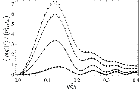
Figure 1: Normalized spectrum of density ripples $\left\langle|\rho(q)|^{2}\right\rangle/(n_{1D}^{2}\xi_{h})$ for weakly interacting 1D quasicondensate of ⁸⁷Rb atoms with density $n_{1D}=40\,\mbox{$\mu$}\mbox{m}^{-1},$ transverse confinement frequency $\omega_{\perp}=2\pi\times 2\,\mbox{kHz},$ Luttinger liquid parameter $K\approx 47,$ and healing length $\xi_{h}\approx 0.37\,\mbox{$\mu$}\mbox{m}.$ Expansion time is fixed at $t=27\,\mbox{ms}$ (with $\frac{1}{\xi_{h}}\sqrt{\frac{\hbar t}{m}}\approx 11.8$), and temperatures equal (top to bottom) $T=40\,\mbox{nK}\,(k_{B}T/\mu=1),\;T=27\,\mbox{nK}\,(k_{B}T/\mu=0.67),$ $T=12\,\mbox{nK}\,(k_{B}T/\mu=0.3),$ and $T=0.$ Values on the axes of this and subsequent plots are dimensionless. Dots are obtained by numerical integration of Eq. (21) in the weakly interacting limit making use of Eqs. (25)-(30). Solid lines correspond to analytical results [Eq. (37)], which are derived under condition (33).

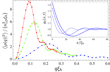
Figure 2: (Color online) Normalized spectrum of density ripples $\left\langle|\rho(q)|^{2}\right\rangle/(n_{1D}^{2}\xi_{h})$ with the same parameters as in Fig. 1 but for a fixed temperature $T=27\mbox{nK}\,(k_{B}T/\mu=0.67),$ and various times of flight: $t=49\mbox{ms}$ (red, solid), $t=27\mbox{ms}$ (green, dashed), and $t=9.5\mbox{ms}$ (blue, dotted). Dots are obtained by numerical integration of Eq. (21) in the weakly interacting limit making use of Eqs. (25)-(30). Lines correspond to analytical results [Eq. (37)], which are derived under condition (33). Inset shows $g_{2}(x;t),$ obtained from $\left\langle|\rho(q)|^{2}\right\rangle$ using the inverse of Eq. (22).

There are several qualitative features that should be noted. The spectrum of density ripples is not a monotonic function, and can also have several maxima. The positions of the maxima only weakly depend on the temperature, and are mostly determined by the expansion time. The amplitude of the ripples, on the other hand, significantly depends both on the expansion time and temperature.

Let us now derive a simple analytical expression for the spectrum of density ripples, which is valid in the regime [justified below after Eq. (39)]

$$\frac{\pi}{\xi_{h}}\sqrt{\frac{\hbar t}{m}}\frac{k_{B}T}{\mu}\gg 1.$$ (33)

Under this condition one can use Eq. (31) and approximate the two-point correlation function by

$$g_{1}(x)\approx\exp{\left(-|x|/\lambda_{T}\right)}\;\mbox{for}\;|x|\gg\xi_{h}\frac{\mu}{k_{B}T},$$ (34)

where $\lambda_{T}$ is defined by

$$\lambda_{T}=\frac{2K\xi_{h}\mu}{\pi k_{B}T}=\frac{2\hbar^{2}n_{1D}}{mk_{B}T},$$ (35)

and does not depend on interaction strength, as long as Eq. (32) is satisfied.

Using Eqs. (25) and (34), the second line of Eq. (21) can be written as

$$\frac{g_{1}(\hbar qt/m)^{2}g_{1}(X)^{2}}{g_{1}(X-\hbar qt/m)g_{1}(X+\hbar qt/m)}\approx\exp{\frac{-X}{\lambda_{T}}}\;\mbox{for}\;X\leq\frac{\hbar qt}{m},$$

$$\mbox{and}\;\exp{\frac{-\hbar qt}{m\lambda_{T}}}\;\mbox{otherwise}.$$

The constant term $\exp{\frac{-\hbar qt}{m\lambda_{T}}}$ is responsible for $g_{2}(x\rightarrow\infty,t)=1.$ Since according to Eq. (21) we need to take a Fourier transform of the above expression, subtracting the constant on the whole interval $(0,\infty)$ does not affect $\left\langle|\rho(q)|^{2}\right\rangle$ for $q\neq 0,$ and we obtain

$$\frac{\left\langle|\rho(q)|^{2}\right\rangle}{n_{1D}^{2}}\approx 2\int_{0}^{\frac{\hbar qt}{m}}dx\cos{qx}\left(\exp{\frac{-x}{\lambda_{T}}}-\exp{\frac{-\hbar qt}{m\lambda_{T}}}\right).$$ (36)

This integral can be evaluated in a closed form, and leads to an analytical answer

$$\frac{\left\langle|\rho(q)|^{2}\right\rangle}{n_{1D}^{2}\xi_{h}}\approx\frac{\lambda_{T}q-e^{\frac{-2\hbar qt}{m\lambda_{T}}}\left(\lambda_{T}q\cos{\frac{\hbar q^{2}t}{m}}+2\sin{\frac{\hbar q^{2}t}{m}}\right)}{q\xi_{h}\left(1+\lambda^{2}_{T}q^{2}\right)}.$$ (37)

Note that the last equation reduces to Eq. (24) when $\lambda_{T}q\gg 1$ and $\hbar qt/m\lambda_{T}\ll 1$. Figures 1 and 2 show an excellent agreement between the analytical result and numerical integration described earlier after Eq. (32). The analytical result shows the same non-monotonic behavior as the numerical calculations. The parameter $\lambda_{T}$ defines a time scale

$$t_{c}\approx 6.5\frac{m\lambda_{T}^{2}}{\hbar}$$ (38)

after which only a single maximum persists. When several maxima and minima are present, their positions can be estimated by

$$\frac{\hbar q^{2}t}{m}\approx\pi(2n-1/2\mp 1/2),$$ (39)

where the upper (lower) sign corresponds to the $n$th maximum (minimum). These conditions can be understood as a “standing wave” conditions in Eq. (36), and become more precise at lower temperatures.

The appearance of minima and maxima in the spectrum of density ripples can be understood in terms of matter-wave near-field diffraction. The analogous effect for light waves (in the spatial domain) is known as the Talbot effect Talbot . Its matter-wave counterpart has been also observed in diffraction of atoms on a grating Talbotnew . In our case, we observe near-field diffraction in the time domain. For each expansion time, a certain momentum contribution will be “imaged” onto itself, leading to a minimum in the spectrum of density ripples for a given momentum $q.$ As compared to diffraction on a regular grating with a fixed period, the typical fluctuation length in the trapped cloud is not constant, but distributed around the thermal length $\lambda_{T}$. Therefore, minima in the spectrum appear for any sufficiently small expansion time, according to condition (39).

Condition (33) can now be justified in the regime where $\left\langle|\rho(q)|^{2}\right\rangle$ is near its largest values. In such case most of the contributions to Eq. (21) come from distances of the order $\sqrt{\hbar t/m},$ and Eq. (33) follows from Eq. (32).

So far we have been assuming that the quasicondensate is deep in the 1D regime, $\mu,k_{B}T\ll\hbar\omega_{\perp}.$ While Eqs. (25)-(30) are valid only under such assumption, Eqs. (34) and (35) also work in the weakly interacting quasi-1D regime,

$$\mu,k_{B}T\sim\hbar\omega_{\perp}.$$ (40)

Indeed, they rely only on the 1D nature of long-range correlations, weakness of interactions, and the property $cK=\pi n_{1D}/m,$ which is a consequence of the Galilean invariance Haldane . In Eqs. (32) and (33), the Luttinger liquid parameter $K$ can be obtained as $K=\hbar\pi n_{1D}/(mc),$ where the square of the sound velocity $c$ can be determined from compressibility as $c^{2}=n_{1D}(\partial{\mu}/\partial{n_{1D}})/m.$ For chemical potential $\mu,$ one can use an approximate relation Gerbier_t $\mu=\hbar\omega_{\perp}(\sqrt{1+4a_{s}n_{1D}}-1).$

Let us now briefly review the conditions under which one can neglect interactions in expanding 1D clouds and the effects of finite condensate length $L.$ Transverse expansion takes place at the times of the order of inverse transverse confinement $\omega_{\perp}^{-1}.$ Up to the times of this order, one cannot neglect interactions during the expansion. Correlation functions which enter Eq. (21) will be smeared up to the distances of the order $\delta x\sim c/\omega_{\perp}=\xi_{h}\mu/\omega_{\perp},$ and smearing will only weakly affect the final result for $\left\langle|\rho(q)|^{2}\right\rangle$ if $q\delta x\ll 1.$ Thus to observe an oscillating spectrum of density ripples, one needs to satisfy the condition

$$\xi_{h}\sqrt{\frac{m}{\hbar t}}\frac{\mu}{\hbar\omega_{\perp}}\ll 1,$$ (41)

which easily holds for the parameters shown in Figs. 1 and 2. In addition, one can use Feshbach resonances Feshbach to completely switch off interactions during the expansion.

Locally, corrections due to finite $L$ can be neglected, if finite limits of integration in Eq. (16) lead to smearing of delta functions up to the distances at which the correlation functions change considerably. This change can occur either because of the variations of the density in external confinement at distances $\sim L,$ or because of the decay of correlations for finite temperatures at distances of the order $\sim K\xi_{h}/a.$ Thus for finite temperatures these conditions read as

$$\frac{mL}{\hbar t}\min{(L,K\xi_{h}/a)}\gg 1,$$ (42)

and are easily satisfied for parameters considered earlier, and, e.g., longitudinal frequency $\omega_{x}=2\pi\times 5\;\mbox{Hz}.$ Under condition (42) one can take the inhomogeneity of the density profile into account within the local-density approximation by averaging the prediction of Eq. (37).

III.2 Strongly interacting 1D Bose gases

Let us now describe the evolution of the two-point density correlation function $g_{2}(x;t)$ of a strongly interacting 1D Bose gas. A dimensionless parameter which controls the strength of interactions at zero temperature can be written as

$$\gamma=\frac{mg_{1D}}{\hbar^{2}n_{1D}}=\frac{2m\omega_{\perp}a_{s}}{\hbar n_{1D}}\gg 1.$$ (43)

Under such conditions, the bosonic wave function takes on fermion properties, and the density correlation function in the trap $g_{2}(x;0)$ is the same as for non-interacting fermions of the same density and temperature. In particular, it vanishes at $x=0,$ and one has $g_{2}(0;0)=0.$ However, the correlation functions that contain creation and annihilation operators at different points, such as $\varrho(x_{1};x_{2};0)$ in Eq. (20), are not the same as for non-interacting fermions. This happens because bosonic operators, when written in terms of fermionic operators, contain a “string” which ensures proper commutation relations.

In the Appendix we derive a representation of $\varrho(x_{1};x_{2};0)$ as a Fredholm-type determinant, which can be easily evaluated numerically. Combining this representation with Eq. (20), we evaluate $g_{2}(x;t)$ after various expansion times numerically. The results for zero temperature are shown in Fig. 3, while the results for finite temperature $k_{B}T=\mu\approx 1.2\frac{\left(\pi\hbar n_{1D}\right)^{2}}{2m}$ are shown in Fig. 4. In spite of a considerable change in the temperature, there is no qualitative change in the behavior of $g_{2}(x;t).$ The qualitative behavior of $g_{2}(x;t)$ in Figs. 3 and 4 is in agreement with Eq. (44) below, and $\lambda_{C}\sim n_{1D}^{-1}$ for the Tonks-Girardeau gas.

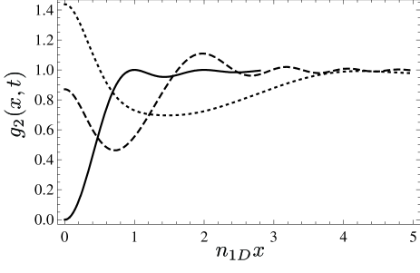
Figure 3: Two-point density correlation function $g_{2}(x;t)$ of a zero-temperature strongly interacting 1D Bose gas (Tonks-Girardeau limit) for different times $t$ after the release of the gas from the trap. Different curves correspond to $t=0$ (solid), $t=0.25m/(\hbar n_{1D}^{2})$ (dashed), and $t=m/(\hbar n_{1D}^{2})$ (dotted).

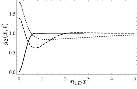
Figure 4: Two-point density correlation function $g_{2}(x;t)$ for the same parameters as in Fig. 3 but for a finite temperature, $k_{B}T=\mu\approx 1.2\frac{\left(\pi\hbar n_{1D}\right)^{2}}{2m}.$

III.3 General remarks about 1D case

Before concluding this section we would like to provide a qualitative analysis of the evolution of the density correlation function $g_{2}(x;t)$ as a function of the expansion time $t$.

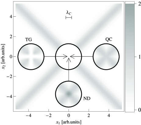
Figure 5: Density plot of the two-particle density matrix $\varrho(x_{1};x_{2};0)$ of a 1D Bose gas, see Eqs. (11) and (17) (the density bar represents the $\varrho$ scale in units of $n_{1D}^{2}$). Initially (at $t=0$) the bosonic system can be a Tonks-Girardeau gas (TG) or a weakly interacting quasicondensate (QC) or a non-degenerate (ND) thermal gas. The central ($x_{1}\approx x_{2}\approx 0$) part of the two-particle density matrix in these cases is shown in three respective insets. The bar shows the typical correlation scale $\lambda_{C}$.

The general structure of the two-particle density matrix $\varrho(x_{1};x_{2};0)$ of a 1D Bose gas is shown schematically in Fig. 5. Because of the Bose symmetry, $\varrho(x_{1};x_{2};0)$ is represented in the $(x_{1},x_{2})$-plane by two infinite perpendicular “bands” of a typical transverse size $\lambda_{C}$ (correlation length). Asymptotically, as $x_{1}\rightarrow\pm\infty$ and $x_{2}=\pm x_{1}$, $\varrho\rightarrow n_{1D}^{2}$. There are several possible cases of atomic correlations near the point $x_{1}=x_{2}=0$ in a trapped 1D gas. In general, at $t=0$, we have $\rho(0;0;0)=n_{1D}^{2}g_{2}(0;0)$. In the case of the Tonks-Girardeau gas of impenetrable bosons Gir ; g1TG $g_{2}(0;0)\equiv g_{2}^{TG}(0)=0$ (at zero temperature $g_{2}^{TG}(x)=1-[\sin(\pi n_{1D}x)/(\pi n_{1D}x)]^{2}$ Gir ). Another possibility is a weakly interacting degenerate gas (quasicondensate), where $g_{2}(0;0)\equiv g^{QC}_{2}(0)\approx 1$ MoraCastin ; g2first ; asg ; g2last ; Deuar . Finally, the 1D Bose gas can be non-degenerate (thermal), in which case $g_{2}(0;0)\equiv g_{2}^{ND}=2$. As the interparticle distance grows, the density correlation function quite rapidly approaches its asymptotic value $g_{2}(x\rightarrow\infty;0)=1$ at the distances of the order of $\lambda_{C}.$

One can show that time-dependent density correlation function can be written as

$$g_{2}(x;t)=1+\kappa(\lambda_{C},x,t)+[g_{2}(0;0)-1]h(\lambda_{C},x,t).$$ (44)

The first term (unity) stems from the band of non-zero values of $\varrho$ aligned along the line $x_{1}=x_{2}$ (see Fig. 5). It represents the density correlation function of an ideal gas of distinguishable particles at equilibrium. The second term, $\kappa(\lambda_{C},x,t)$, reflects the Bose-Einstein statistics of the atoms and appears due to the second band along $x_{2}=-x_{1}$. Its maximum value, $\kappa(\lambda_{C},0,t)$, increases from 0 to 1 on a typical time scale $\sim m\lambda_{C}^{2}/\hbar$. As $|x|$ grows, this term asymptotically approaches 0 on a length scale given by $\lambda_{C}.$ The third term describes washing-out of initial short-range (microscopic) correlations. The maximum value of $h(\lambda_{C},x,t)$ is reached at $x=0$, it decreases from 1 to 0 on a time scale $\sim m\lambda_{C}^{2}/\hbar$, and $h(\lambda_{C},x,t)\approx 0$ if $|x|\gg\lambda_{C}$. In the course of free evolution, the density correlation properties of an expanding Bose gas become similar to that of an ideal Bose gas at temperature $k_{B}T\sim\hbar^{2}/(m\lambda_{C}^{2})$.

IV 2D Bose gases below the Berezinskii-Kosterlitz-Thouless temperature

Let us now discuss the properties of density ripples in expanding 2D clouds. Recently 2D condensates have been realized experimentally in several groups gorlitz ; Zoran_KT ; Clade ; 2dconds ; Kruger ; JILA . Reduced dimensionality has dramatic effect on thermal fluctuations. In the case of 2D Bose gases there is no true long-range order for any finite temperature  MWH . For uniform 2D Bose clouds at sufficiently low temperatures, the two-point correlation function behaves at large distances as Kadanoff ; Popov ; Petrov2D_PRL ; Petrov_review

$$\left\langle\hat{\psi}^{\dagger}({\bf r},0)\hat{\psi}(0,0)\right\rangle\approx n_{2D}\left(\frac{\lambda_{2D}}{r}\right)^{\eta}\;\mbox{for}\;r\gg\lambda_{2D}.$$ (45)

For weakly interacting 2D Bose gas at small temperatures, one can evaluate parameters of Eq. (45) from microscopic theory. The dimensionless parameter characterizing weakness of interactions is written as Petrov2D_PRL ; Petrov_review

$$\tilde{g}=a_{s}\sqrt{\frac{8\pi m\omega_{\perp}}{\hbar}}\ll 1.$$ (46)

The exponent $\eta$ in Eq. (45) equals Petrov2D_PRL ; Petrov_review

$$\eta=\frac{T}{T_{d}}\ll 1\;\;\mbox{for}\;k_{B}T\ll k_{B}T_{d}=\frac{2\pi\hbar^{2}n_{2D}}{m},$$ (47)

and $\lambda_{2D}$ equals the de Broglie wavelength of thermal phonons $\hbar c/(k_{B}T)$ at $k_{B}T\ll\mu,$ and the two-dimensional healing length $\xi_{2D}=\hbar/\sqrt{m\mu}$ at high temperatures $k_{B}T\gg\mu.$

Equation (45) remains valid for $\eta$ smaller than

$$\eta_{c}=1/4,$$ (48)

at which point the BKT Berezinskii ; KT ; GNT transition takes place due to proliferation of vortices, and correlation functions start to decay exponentially with distance.

Such a transition for ultracold 2D Bose gases has been observed recently Zoran_KT ; Clade ; JILA , and its microscopic origin has been elucidated. Experiments of Ref. Zoran_KT studied interference of two independent 2D Bose clouds, which requires imaging along the “in-plane” direction and inevitably leads to averaging over inhomogeneous densities. Study of the spectrum of density ripples in expanding clouds with imaging in transverse direction (as done in Ref. Clade ) avoids this problem altogether, and can provide access to properties of correlations at fixed density. The interplay between the BKT transition and the effects of the external confinement is a rather complicated question even for weakly interacting Bose gas Kruger ; Hadzi_NJP ; Holzmann ; 2DRMP , and we will only discuss the uniform case here.

Even for weak interactions, one cannot use quasicondensate theory to analytically describe correlations as functions of microscopic parameters in the vicinity of the BKT transition or to predict the transition temperature, and has to resort to fully numerical methods Prokofiev . Nevertheless, the factorization property [Eq. (25)] remains valid for large-distance behavior of correlation functions for all $\eta$ below the critical value $1/4,$ since large-distance fluctuations of the phase are still described by the Gaussian theory. Using that together with Eq. (45), we will now obtain the prediction for the spectrum of density ripples which is valid as long as only points with relative distances much larger than $\lambda_{2D}$ contribute significantly to the integral in Eq. (23). We will show below, that this regime is realized if

$$\sqrt{\frac{\hbar t}{m}}\gg\lambda_{2D}.$$ (49)

We introduce a dimensionless variable

$$y=\frac{\hbar q^{2}t}{m},$$ (50)

and use expression Eq. (45) for all ${\bf r}.$ Using symmetries of the resulting integral, the expression for $\left\langle|\rho(q)|^{2}\right\rangle$ is written as

$$\left\langle|\rho(q)|^{2}\right\rangle\approx n_{2D}^{2}\lambda_{2D}^{2}\left(\frac{\hbar t}{m\lambda^{2}_{2D}}\right)^{1-\eta}F(\eta,y),$$ (51)

where $F(\eta,y)$ is a dimensionless function defined by  fnote

$$F(\eta,y)=\frac{4}{y^{1+\eta}}\int_{0}^{\infty}dr_{x}\cos{r_{x}}\int_{0}^{\infty}dr_{y}$$

$$\left\{\left[\frac{\sqrt{(r_{x}+y)^{2}+r_{y}^{2}}\sqrt{(r_{x}-y)^{2}+r_{y}^{2}}}{r_{x}^{2}+r_{y}^{2}}\right]^{\eta}-1\right\}.$$ (52)

We find that the spectrum of density ripples remains self-similar in the course of expansion and the shape of the spectrum is a function of $\eta$ only. Plots of $F(\eta,y)$ for three different values of $\eta$ are shown in Fig. 6, and have a similar structure. Positions of maxima and minima are very well described by Eq. (39), where the upper (lower) sign corresponds to the $n$th maximum (minimum). In Eq. (23) typical distances which contribute to $\left\langle|\rho(q)|^{2}\right\rangle$ near its maximum at $y\approx\pi$ can be estimated as $\sim\sqrt{\hbar t/m},$ which leads to condition (49). Note however, that self-similarity starts breaking down for sufficiently large $y$ even when condition (49) is satisfied.

Scaling of the magnitude of $\left\langle|\rho(q)|^{2}\right\rangle$ with time in the self-similar regime can be used to extract $\eta.$ For example, the integral of $\left\langle|\rho(q)|^{2}\right\rangle$ from zero to its first minimum scales with time as

$$\int_{0}^{\sqrt{\frac{2\pi m}{\hbar t}}}dq\left\langle|\rho(q)|^{2}\right\rangle\propto t^{1/2-\eta},$$ (53)

and the exponent changes considerably as $\eta$ changes from $0$ to the critical value $1/4.$

For small $\eta,$ one can derive an expansion of $F(\eta,y)$ as

$$F(\eta,y)=\frac{4}{y^{1+\eta}}\left[\eta f_{1}(y)+\eta^{2}f_{2}(y)+\eta^{3}f_{3}(y)+...\right],$$ (54)

where $f_{1}(y)$ can be evaluated analytically as

$$f_{1}(y)=2\pi\sin^{2}{\frac{y}{2}}.$$ (55)

The term $f_{2}(y)$ leads to a finite value of $F(\eta,y)$ at the first minimum. By including effects of $f_{2}(y)$ and $f_{3}(y),$ one can derive

$$\frac{F(\eta,2\pi)}{F(\eta,\pi)}\approx\frac{1}{2^{\eta}}\left(1.19\eta+0.38\eta^{2}\right)\;\mbox{for}\;\eta\ll 1,$$ (56)

which coincides with the direct numerical evaluation up to $2.5\%$ for $\eta=0.25.$

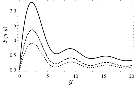
Figure 6: Dependence of universal functions $F(\eta,y)$ on $y=\frac{\hbar q^{2}t}{m}$ plotted for three different values of correlation exponents $\eta.$ Under condition (49) functions $F(\eta,y)$ determine the self-similar shape of the spectrum of density ripples according to Eq. (51). Curves from top to bottom correspond to $\eta=0.25$ (solid, the Berezinskii-Kosterlitz-Thouless point), $\eta=0.15$ (dashed), and $\eta=0.10$ (dotted).

For weakly interacting uniform 2D Bose gases at low temperatures, one can also obtain predictions which are not limited by Eq. (49). Under condition

$$n_{2D}\xi_{2D}^{2}\gg 1$$ (57)

an extension of Bogoliubov theory to 2D quasicondensates describes correlations at all distances MoraCastin . Such a theory is valid up to temperatures of the order

$$\frac{k_{B}T}{\mu}\log{\frac{k_{B}T}{\mu}}\sim n_{2D}\xi_{2D}^{2}\gg 1,$$ (58)

and predicts the exponent (47). The correlation function is written as

$$g_{1}({\bf r})=\frac{\left\langle\hat{\psi}^{\dagger}({\bf r},0)\hat{\psi}(0,0)\right\rangle}{n_{2D}}=\exp{\left[-\frac{2\pi\mu}{k_{B}T_{d}}f_{2D}\left(\frac{r}{\xi_{2D}}\right)\right]},$$

where the dimensionless function $f_{2D}(s)$ is defined by

$$f_{2D}(s)=\int_{0}^{\infty}\frac{kdk}{2\pi}\left[1-J_{0}({ks})\right]\left\{\right[u_{k}^{2}+v_{k}^{2}\left]n_{k}+v_{k}^{2}\right\}.$$

Here, $J_{0}(x)$ is the Bessel function, and $u_{k},v_{k}$ and $n_{k}$ are defined by Eqs. (28)-(30).

We now consider a case of ⁸⁷Rb atoms with transverse confinement frequency $\omega_{\perp}=2\pi\times 3\,\mbox{kHz},$ and density $n_{2D}\approx 84\,\mbox{$\mu$}\mbox{m}^{-2}.$ This yields the dimensionless interaction parameter $\tilde{g}\approx 0.13,$ healing length $\xi_{h}\approx 0.3\,\mbox{$\mu$}\mbox{m},$ and $n_{2D}\xi_{2D}^{2}\approx 7.5.$ We perform a numerical integration of Eq. (23) for temperature $T=60\,\mbox{nK}\,$(which corresponds to correlation exponent $0.02$) and various expansion times, and the results are shown in Fig. 7.

Qualitatively, they look similar to the self-similar regime for all times, and one again obtains an oscillating spectrum of density ripples with maxima and minima very well described by Eq. (39). In the weakly interacting regime the ratio of the first maximum to the first minimum for $\left\langle|\rho(q)|^{2}\right\rangle$ is much larger than one, similar to the weakly interacting 1D Bose gas.

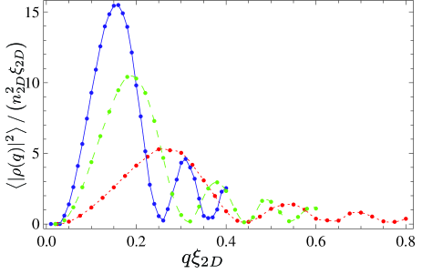
Figure 7: (Color online) Normalized spectrum of density ripples $\left\langle|\rho(q)|^{2}\right\rangle/(n_{2D}^{2}\xi_{2D})$ for weakly interacting 2D quasicondensate of ⁸⁷Rb atoms with density $n_{2D}\approx 84\,\mbox{$\mu$}\mbox{m}^{-2},$ transverse confinement frequency $\omega_{\perp}=2\pi\times 3\,\mbox{kHz},$ healing length $\xi_{h}\approx 0.3\,\mbox{$\mu$}\mbox{m},$ and dimensionless interaction parameter $\tilde{g}\approx 0.13.$ Temperature is taken to be $T=60\,\mbox{nK}\,(k_{B}T\approx\mu),$ which corresponds to correlation exponent $\eta=0.020.$ Various curves correspond to expansion times $t=12\,\mbox{ms}$ (blue, solid), $t=8\,\mbox{ms}$ (green, dashed), and $t=4\,\mbox{ms}$ (red, dotted). The lines are guides to the eyes.

V Conclusions

To conclude, we calculated the evolution of the two-point density correlation function of an ultracold atomic Bose gas released from a tight transverse confinement.

For 1D gases in the weakly interacting regime, in a wide range of parameters given by Eq. (33), we analytically calculated the spectrum of density ripples $\left\langle|\rho(q)|^{2}\right\rangle.$ Our results are summarized in Eq. (37) and Figs. 1 and 2. Our analytical theory is also applicable in the quasi-1D regime when $k_{B}T$ and $\mu$ are of the order of transverse confinement frequency $\hbar\omega_{\perp}.$ For expansion times smaller than $6.5m\lambda_{T}^{2}/\hbar,$ we find that the spectrum of density ripples can have several maxima and minima, and their positions can be estimated using Eq. (39). While positions of maxima and minima are essentially independent of the temperature, their amplitude exhibits strong temperature dependence. For 1D quasicondensates, the density profile in external harmonic confinement depends weakly on the temperature, when the latter is of the order of the chemical potential MoraCastin . The density profile follows the inverted parabola shape Pollet , thus the bimodal density fitting cannot be used to measure temperatures reliably. We propose that our analytical result Eq. (37) can be used for thermometry of one-dimensional systems. Experimental investigation of this question is currently under way, and will be presented in a separate presentation Manz .

For one-dimensional systems, we also discussed evolution of the density correlation function in real space, $g_{2}(x;t)$. For long expansion times we find that the correlation function $g_{2}(x;t)$ reaches the value of $2$ at short distances and approaches the value $1$ for distances larger than the correlation length, see, e.g., Fig. 3 for Tonks-Girardeau regime.

For 2D Bose gases with temperatures below the Berezinskii-Kosterlitz-Thouless transition and sufficiently long expansion time, we showed that the spectrum of the density ripples evolves in a self-similar way. Our result for this case is given in Eq. (51) and Fig. 6, with positions of maxima and minima determined by Eq. (39). The scaling of the overall magnitude can be used to extract the correlation exponent $\eta,$ e.g., using Eq. (53).

For more complicated situations, e.g., multicomponent gases, relation (21) and its cross-correlation generalizations can be used as a convenient experimental tool to characterize complex many-body states and their correlations. In addition, it can be used as an experimental tool to investigate non-equilibrium phenomena in low-dimensional gases.

A.I. was supported by DOE Grant No. DE-FG02-08ER46482. I.E.M. acknowledges support through the Lise Meitner program by the FWF, and the INTAS. D.S.P. was supported by ANR Grant No. 08-BLAN-0165-01 and by the Russian Foundation for Fundamental Research. V.G. was supported by Swiss National Science Foundation. S.M. acknowledges support from the FWF doctoral program CoQuS. T.S. acknowledges support by the FWF program P21080.E.D. was supported by the NSF Grant No. DMR-0705472, DARPA, MURI, and Harvard-MIT CUA. J.S. was supported by the EC, and the FWF. We acknowledge useful discussions with A. Aspect, P. Cladé, E. Cornell, J. Dalibard, N. J. van Druten, M. Greiner, Z. Hadzibabic, K. Kheruntsyan, and W. Phillips.

Appendix A Two-particle density matrix of a strongly interacting 1D Bose gas

In this appendix we will describe a Fredholm-type determinant representation for $\varrho(x_{1};x_{2};0)$ for $0<x_{1}<x_{2},$ which can be easily evaluated numerically. Due to Eqs. (18) and (19) this defines $\varrho(x_{1};x_{2};0)$ for any values of $x_{1}$ and $x_{2}.$ Representations similar to the one developed here can be obtained for any multi-point correlation function of bosonic fields in the strongly interacting limit.

Mathematically, fermionization can be written as

$$\hat{\psi}^{{\dagger}}(x)=\exp{\left[i\pi\int^{x-0}_{-\infty}dy\,\hat{\psi}_{f}^{{\dagger}}(y)\hat{\psi}_{f}(y)\right]}\hat{\psi}_{f}^{{\dagger}}(x),$$ (59)

$$\hat{\psi}(x)=\exp{\left[-i\pi\int^{x-0}_{-\infty}dy\,\hat{\psi}_{f}^{{\dagger}}(y)\hat{\psi}_{f}(y)\right]}\hat{\psi}_{f}(x),$$ (60)

where we introduced fermionic creation and annihilation operators $\hat{\psi}_{f}^{{\dagger}}(x)$ and $\hat{\psi}_{f}(x),$ which have standard anti-commutation relations

$$\left\{\hat{\psi}_{f}^{{\dagger}}(x),\hat{\psi}_{f}(y)\right\}=\delta(x-y),$$ (61)

$$\left\{\hat{\psi}_{f}^{{\dagger}}(x),\hat{\psi}^{{\dagger}}_{f}(y)\right\}=\left\{\hat{\psi}_{f}(x),\hat{\psi}_{f}(y)\right\}=0.$$ (62)

For zero temperature, ground state for fermions corresponds to a filled Fermi sea, whereas at finite temperature one should use a thermal density matrix for non-interacting fermions.

For convenience, we will introduce a fictitious underlying lattice of spacing $a\ll x_{1},x_{2},$ such that

$$\frac{x_{1}}{2}\frac{1}{a}=m_{1}\gg 1,$$ (63)

$$\frac{x_{2}}{2}\frac{1}{a}=m_{2}>m_{1}\gg 1,$$ (64)

where $m_{1}$ and $m_{2}$ are large positive integer numbers. At the end of the calculation, we will take the limit $a\rightarrow 0$ such that $m_{1}a\rightarrow x_{1}/2,m_{2}a\rightarrow x_{2}/2.$ On a lattice, fermionization rules [Eqs. (59) and (60)] and commutation relations (61) and (62) are written as

$$\hat{\psi}^{{\dagger}}(i)=\prod_{k<i}\left[1-2\hat{\psi}_{f}^{{\dagger}}(k)\hat{\psi}_{f}(k)\right]\hat{\psi}_{f}^{{\dagger}}(i),$$ (65)

$$\hat{\psi}(i)=\prod_{k<i}\left[1-2\hat{\psi}_{f}^{{\dagger}}(k)\hat{\psi}_{f}(k)\right]\hat{\psi}_{f}(i),$$ (66)

$$\left\{\hat{\psi}_{f}^{{\dagger}}(i),\hat{\psi}_{f}(k)\right\}=\delta_{ik},$$ (67)

$$\left\{\hat{\psi}_{f}^{{\dagger}}(i),\hat{\psi}^{{\dagger}}_{f}(k)\right\}=\left\{\hat{\psi}_{f}(i),\hat{\psi}_{f}(k)\right\}=0.$$ (68)

Using these relations, $\varrho(x_{1};x_{2};0)$ can be written as

$$\varrho(x_{1};x_{2};0)=\left\langle\hat{\psi}_{f}^{{\dagger}}(m_{1})\hat{\psi}_{f}^{{\dagger}}(-m_{1})\right.$$

$$\times\left.\prod_{k\in S}\left[1-2\hat{\psi}_{f}^{{\dagger}}(k)\hat{\psi}_{f}(k)\right]\hat{\psi}_{f}(m_{2})\hat{\psi}_{f}(-m_{2})\right\rangle,$$ (69)

where subset $S$ equals

$$S=\left[-m_{2}+1,-m_{1}-1\right]\bigcup\left[m_{1}+1,m_{2}-1\right].$$ (70)

Expanding the parentheses, we obtain

$$\varrho(x_{1};x_{2};0)=\left\langle\sum_{n=0}^{\infty}(-2)^{n}\hat{\psi}_{f}^{{\dagger}}(m_{1})\hat{\psi}_{f}^{{\dagger}}(-m_{1})\right.$$

$$\times\sum_{j_{1}<...<j_{n},j_{k}\in S}\hat{\psi}_{f}^{{\dagger}}(j_{1})...\hat{\psi}_{f}^{{\dagger}}(j_{n})\hat{\psi}_{f}(j_{n})...\hat{\psi}_{f}(j_{1})$$

$$\times\left.\hat{\psi}_{f}(m_{2})\hat{\psi}_{f}(-m_{2})\right\rangle.$$ (71)

For each $n$ and set of $j_{1},...,j_{n},$ expectation value of $n+2$ creation and $n+2$ annihilation operators can be written using Wick’s theorem AGD as a determinant of $(n+2)\times(n+2)$ matrix Burovskii ; Zvonarev_string

$$M^{(n+2)}_{i,j}=aG(s_{i},t_{j}),$$ (72)

where

$$s_{1}=-m_{1}a,\;s_{2}=m_{1}a,\;s_{i>2}=j_{i-2}a,$$ (73)

$$t_{1}=m_{2}a,\;t_{2}=-m_{2}a,\;t_{i>2}=j_{i-2}a,$$ (74)

and $G(x,y)=G(x-y)$ is a Green’s function of a free Fermi gas, which e.g. for zero temperature equals

$$G(x)=\int_{-k_{f}}^{k_{f}}\exp{\left[ikx\right]}\frac{dk}{2\pi}=\frac{\sin{\pi n_{1D}x}}{\pi x}.$$ (75)

Since the structure of the matrix $M^{(n+2)}_{i,j}$ does not depend on $n,$ summation over different $n$ and sets $j_{1},...,j_{n}$ can be now represented as a single Fredholm-type determinant Zvonarev_string ; Smirnov_book

$$\varrho(x_{1};x_{2};0)=\frac{\mbox{Det}\;\left[A_{ij}-2aB_{ij}\right]}{4a^{2}},$$ (76)

where matrices $A_{ij}$ and $B_{ij}$ of size $2(m_{2}-m_{1})\times 2(m_{2}-m_{1})$ are defined by

$$A_{ij}=\,\mbox{Diag}\{0,0,1,...,1\},$$ (77)

$$B_{ij}=G(\tilde{s}_{i},\tilde{t}_{j}),$$ (78)

and

$$\tilde{s}_{1}=-m_{1}a,\;\tilde{s}_{2}=m_{1}a,$$ (79)

$$\tilde{s}_{i}=\left(-m_{2}+i-2\right)a\;\mbox{for}\;3\leq i<2+m_{2}-m_{1},$$ (80)

$$\tilde{s}_{i}=\left(2m_{1}-m_{2}+i-1\right)a\;\mbox{for}$$

$$\;2+m_{2}-m_{1}\leq i\leq 2(m_{2}-m_{1}),$$ (81)

$$\tilde{t}_{1}=m_{2}a,\;\tilde{t}_{2}=-m_{2}a,\;\tilde{t}_{i>2}=\tilde{s}_{i}.$$ (82)

Expansion of the determinant of $A_{ij}-2aB_{ij}$ using the rule for the determinant of the sum of two matrices (see, e.g., p. 221 of Ref. KBI ) generates the expansion of Eq. (71), similar to a usual Fredholm determinant Smirnov_book . Indeed, only diagonal minors not including lines $1$ and $2$ can be chosen from the matrix $A_{ij}.$ Complimentary minor of size $(n+2)\times(n+2)$ from the matrix $B_{ij}$ is proportional to matrix $M^{(n+2)}$ in Eq. (72), and the summation over possible different sets of $j_{1},...,j_{n}$ is equivalent to a summation over different partitions of matrix $A_{ij}$ into diagonal minors.

Since determinants are easy to evaluate numerically, one can now take the limit $a\rightarrow 0$ numerically and evaluate $\varrho(x_{1};x_{2};0)$ with any precision.

References

- (1) M. Greiner, O. Mandel, T. Esslinger, T. W. Hänsch, and I. Bloch, Nature (London) 415, 39 (2002).
- (2) U. Schneider, L. Hackermüller, S. Will, Th. Best, I. Bloch, T. A. Costi, R. W. Helmes, D. Rasch, and A. Rosch, Science 322, 1520 (2008).
- (3) A. Perrin, H. Chang, V. Krachmalnicoff, M. Schellekens, D. Boiron, A. Aspect, and C. I. Westbrook, Phys. Rev. Lett. 99, 150405 (2007).
- (4) S. Hofferberth, I. Lesanovsky, B. Fischer, T. Schumm, and J. Schmiedmayer, Nature (London) 449, 324 (2007).
- (5) S. Hofferberth, I. Lesanovsky, T. Schumm, A. Imambekov, V. Gritsev, E. Demler, and J. Schmiedmayer, Nat. Phys. 4, 489 (2008).
- (6) V. L. Berezinskii, Sov. Phys. JETP 32, 493 (1971); 34, 610 (1972).
- (7) J. M. Kosterlitz and D. J. Thouless, J. Phys. C 6, 1181 (1973); J. M. Kosterlitz, ibid. 7, 1046 (1974).
- (8) Z. Hadzibabic, P. Krüger, M. Cheneau, B. Battelier, and J. Dalibard, Nature (London) 441, 1118 (2006).
- (9) M. Schellekens, R. Hoppeler, A. Perrin, J. Viana Gomes, D. Boiron, A. Aspect, and C. I. Westbrook, Science 310, 648 (2005).
- (10) T. Jeltes, J. M. McNamara, W. Hogervorst, W. Vassen, V. Krachmalnicoff, M. Schellekens, A. Perrin, H. Chang, D. Boiron, A. Aspect, and C. I. Westbrook, Nature (London) 445, 402 (2007).
- (11) S. Fölling, F. Gerbier, A. Widera, O. Mandel, T. Gericke, and I. Bloch, Nature (London) 434, 481 (2005).
- (12) T. Rom, Th. Best, D. van Oosten, U. Schneider, S. Fölling, B. Paredes, and I. Bloch, Nature (London) 444, 733 (2006).
- (13) A. Öttl, S. Ritter, M. Köhl, and T. Esslinger, Phys. Rev. Lett. 95, 090404 (2005).
- (14) F. Schreck, L. Khaykovich, K. L. Corwin, G. Ferrari, T. Bourdel, J. Cubizolles, and C. Salomon, Phys. Rev. Lett. 87, 080403 (2001).
- (15) A. Görlitz, J. M. Vogels, A. E. Leanhardt, C. Raman, T. L. Gustavson, J. R. Abo-Shaeer, A. P. Chikkatur, S. Gupta, S. Inouye, T. Rosenband, and W. Ketterle, Phys. Rev. Lett. 87, 130402 (2001).
- (16) T. Kinoshita, T. Wenger and D. S. Weiss, Science 305, 1125 (2004).
- (17) B. Paredes, A. Widera, V. Murg, O. Mandel, S. Fölling, I. Cirac, G. V. Shlyapnikov, T. W. Hänsch, and I. Bloch, Nature (London) 429, 277 (2004).
- (18) J.-B. Trebbia, J. Esteve, C. I. Westbrook, and I. Bouchoule, Phys. Rev. Lett. 97, 250403 (2006).
- (19) A. H. van Amerongen, J. J. P. van Es, P. Wicke, K. V. Kheruntsyan, and N. J. van Druten, Phys. Rev. Lett. 100, 090402 (2008).
- (20) I. Bouchoule, N. J. Van Druten, C. I. Westbrook, arXiv:0901.3303v2.
- (21) T. Kinoshita, T. Wenger, and D. S. Weiss, Phys. Rev. Lett. 95, 190406 (2005).
- (22) B. Laburthe Tolra, K. M. O’Hara, J. H. Huckans, W. D. Phillips, S. L. Rolston, and J. V. Porto, Phys. Rev. Lett. 92, 190401 (2004).
- (23) Yu. Kagan, B. V. Svistunov, and G. V. Shlyapnikov, JETP Lett. 42, 209 (1985).
- (24) Y. Miroshnychenko, W. Alt, I. Dotsenko, L. Förster, D. Meschede, D. Schrader, M. Khudaverdyan, and A. Rauschenbeutel, Nature (London) 442, 151 (2006).
- (25) Y. Colombe, T. Steinmetz, G. Dubois, F. Linke, D. Hunger, and J. Reichel, Nature (London) 450, 272 (2007).
- (26) K. D. Nelson, X. Li, and D. S. Weiss, Nat. Phys. 3, 556 (2007).
- (27) T. Gericke, P. Würtz, D. Reitz, T. Langen, and H. Ott, Nat. Phys. 4, 949 (2008).
- (28) M. Wilzbach, D. Heine, S. Groth, X. Liu, T. Raub, B. Hessmo, and J. Schmiedmayer, Opt. Lett. 34, 259 (2009).
- (29) D. Heine, M. Wilzbach, T. Raub, B. Hessmo, and J. Schmiedmayer, Phys. Rev. A 79, 021804(R) (2009).
- (30) D. S. Petrov, G. V. Shlyapnikov, and J. T. M. Walraven, Phys. Rev. Lett. 87, 050404 (2001).
- (31) S. Dettmer, D. Hellweg, P. Ryytty, J. J. Arlt, W. Ertmer, K. Sengstock, D. S. Petrov, G. V. Shlyapnikov, H. Kreutzmann, L. Santos, and M. Lewenstein, Phys. Rev. Lett. 87, 160406 (2001).
- (32) D. Hellweg, S. Dettmer, P. Ryytty, J. J. Arlt, W. Ertmer, K. Sengstock, D. S. Petrov, G. V. Shlyapnikov, H. Kreutzmann, L. Santos, and M. Lewenstein, Appl. Phys. B: Lasers Opt. 73, 781 (2001).
- (33) H. Kreutzmann, A. Sanpera, L. Santos, M. Lewenstein, D. Hellweg, L. Cacciapuoti, M. Kottke, T. Schulte K. Sengstock, J. J. Arlt, and W. Ertmer, Appl. Phys. B: Lasers Opt. 76, 165 (2003).
- (34) J. Viana Gomes, A. Perrin, M. Schellekens, D. Boiron, C. I. Westbrook, and M. Belsley, Phys. Rev. A 74, 053607 (2006).
- (35) L. S. Cederbaum, A. I. Streltsov, Y. B. Band, and O. E. Alon, Phys. Rev. Lett. 98, 110405 (2007).
- (36) O. E. Alon, A. I. Streltsov, and L. S. Cederbaum, Phys. Lett. A 373, 301 (2009).
- (37) P. Öhberg and L. Santos, Phys. Rev. Lett. 89, 240402 (2002); P. Pedri, L. Santos, P. Öhberg, and S. Stringari, Phys. Rev. A 68, 043601 (2003).
- (38) M. Rigol and A. Muramatsu, Phys. Rev. Lett. 93, 230404 (2004); 94, 240403 (2005); Mod. Phys. Lett. B 19, 861 (2005).
- (39) A. Minguzzi and D. M. Gangardt, Phys. Rev. Lett 94, 240404 (2005).
- (40) M. Rigol, V. Dunjko, V. Yurovsky, and M. Olshanii, Phys. Rev. Lett. 98, 050405 (2007).
- (41) D. M. Gangardt and M. Pustilnik, Phys. Rev. A 77, 041604(R) (2008).
- (42) H. Buljan, R. Pezer, and T. Gasenzer, Phys. Rev. Lett. 100, 080406 (2008); 102, 049903(E) (2009).
- (43) D. Jukić, R. Pezer, T. Gasenzer, and H. Buljan, Phys. Rev. A 78, 053602 (2008).
- (44) D. Jukić, B. Klajn, and H. Buljan, Phys. Rev. A 79, 033612 (2009).
- (45) A. del Campo and J. G. Muga, Europhys. Lett. 74, 965 (2006).
- (46) M. Girardeau, J. Math. Phys. 1, 516 (1960).
- (47) N. Bogoliubov, J. Phys. (Moscow) 11, 23 (1947).
- (48) L. Pitaevskii and S. Stringari, Bose-Einstein Condensation (Oxford University Press, New York, 2003).
- (49) C. J. Pethick and H. Smith, Bose-Einstein Condensation in Dilute Gases (Cambridge University Press, Cambridge, England, 2001).
- (50) S. Inouye, M. R. Andrews, J. Stenger, H.-J. Miesner, D. M. Stamper-Kurn, and W. Ketterle, Nature (London) 392, 151 (1998); Ph. Courteille, R. S. Freeland, D. J. Heinzen, F. A. van Abeelen, and B. J. Verhaar, Phys. Rev. Lett. 81, 69 (1998); J. L. Roberts, N. R. Claussen, J. P. Burke, Jr., C. H. Greene, E. A. Cornell, and C. E. Wieman, ibid. 81, 5109 (1998).
- (51) N. D. Mermin and H. Wagner, Phys. Rev. Lett. 17, 1133 (1966); P. C. Hohenberg, Phys. Rev. 158, 383 (1967).
- (52) S. Coleman, Commun. Math. Phys. 31, 259 (1973).
- (53) P. D. Naselsky, D. I. Novikov, and I. D. Novikov, The Physics of the Cosmic Microwave Background (Cambridge University Press, Cambridge, England, 2006).
- (54) J. C. Mather, Rev. Mod. Phys. 79, 1331 (2007); G. F. Smoot, ibid. 79, 1349 (2007).
- (55) T. Padmanabhan, Structure Formation in the Universe (Cambridge University Press, Cambridge, England, 1993).
- (56) L. J. Garay, J. R. Anglin, J. I. Cirac, and P. Zoller, Phys. Rev. Lett. 85, 4643 (2000).
- (57) G. E. Volovik, Universe in a Helium Droplet (Oxford University Press, Oxford, 2003).
- (58) P. O. Fedichev and U. R. Fischer, Phys. Rev. A 69, 033602 (2004).
- (59) C. Barceló, S. Liberati, and M. Visser, Living Rev. Relativ. 8, 12 (2005).
- (60) M. Uhlmann, Y. Xu, and R. Schützhold, New J. Phys. 7, 248 (2005).
- (61) R. Balbinot, A. Fabbri, S. Fagnocchi, A. Recati, and I. Carusotto, Phys. Rev. A 78, 021603(R) (2008).
- (62) I. Carusotto, S. Fagnocchi, A. Recati, R. Balbinot, and A. Fabbri, New J. Phys. 10, 103001 (2008).
- (63) M. Uhlmann, Phys. Rev. A 79, 033601 (2009).
- (64) D. Hellweg, L. Cacciapuoti, M. Kottke, T. Schulte, K. Sengstock, W. Ertmer, and J. J. Arlt, Phys. Rev. Lett. 91, 010406 (2003); L. Cacciapuoti, D. Hellweg, M. Kottke, T. Schulte, W. Ertmer, J. J. Arlt, K. Sengstock, L. Santos, and M. Lewenstein, Phys. Rev. A 68, 053612 (2003).
- (65) F. Gerbier, J. H. Thywissen, S. Richard, M. Hugbart, P. Bouyer, and A. Aspect, Phys. Rev. A 67, 051602(R) (2003).
- (66) S. Richard, F. Gerbier, J. H. Thywissen, M. Hugbart, P. Bouyer, and A. Aspect, Phys. Rev. Lett. 91, 010405 (2003).
- (67) M. Hugbart, J. Retter, F. Gerbier, A. Varon, S. Richard, J. Thywissen, D. Clement, P. Bouyer, and A. Aspect, Eur. Phys. J. D 35, 155 (2005).
- (68) P. Cladé, C. Ryu, A. Ramanathan, K. Helmerson, and W. D. Phillips, Phys. Rev. Lett. 102, 170401 (2009).
- (69) E. Altman, E. Demler, and M. D. Lukin, Phys. Rev. A 70, 013603 (2004).
- (70) J. Esteve, J.-B. Trebbia, T. Schumm, A. Aspect, C. I. Westbrook, and I. Bouchoule, Phys. Rev. Lett. 96, 130403 (2006).
- (71) A. Polkovnikov, E. Altman, and E. Demler, Proc. Natl. Acad. Sci. U.S.A. 103, 6125 (2006).
- (72) V. Gritsev, E. Altman, E. Demler and A. Polkovnikov, Nat. Phys. 2 , 705 (2006).
- (73) A. Imambekov, V. Gritsev, and E. Demler, Phys. Rev. A 77, 063606 (2008).
- (74) A. Imambekov, V. Gritsev, and E. Demler, in Ultracold Fermi Gases, Proceedings of the International School of Physics “Enrico Fermi”, 2006 (IOS, Amsterdam, The Netherlands, 2007); arXiv:cond-mat/0703766v1.
- (75) V. N. Popov, Theor. Math. Phys. 11, 565 (1972); Functional Integrals in Quantum Field Theory and Statistical Physics (Reidel, Dordrecht, 1983).
- (76) D. S. Petrov, G. V. Shlyapnikov, and J. T. M. Walraven, Phys. Rev. Lett. 85, 3745 (2000).
- (77) C. Mora and Y. Castin, Phys. Rev. A 67, 053615 (2003); Y. Castin, J. Phys. IV 116, 89 (2004).
- (78) C. Gils, L. Pollet, A. Vernier, F. Hebert, G. G. Batrouni, and M. Troyer, Phys. Rev. A 75, 063631 (2007).
- (79) C. N. Yang and C. P. Yang, J. Math. Phys. 10, 1115 (1969).
- (80) K. B. Efetov and A. I. Larkin, Sov. Phys. JETP 42, 390 (1975).
- (81) F. D. M. Haldane, Phys. Rev. Lett. 47, 1840 (1981).
- (82) M. A. Cazalilla, J. Phys. B 37, S1 (2004).
- (83) J. O. Andersen, U. Al Khawaja, and H. T. C. Stoof, Phys. Rev. Lett. 88, 070407 (2002).
- (84) U. Al Khawaja, J. O. Andersen, N. P. Proukakis, and H. T. C. Stoof, Phys. Rev. A 66, 013615 (2002).
- (85) D. S. Petrov, D. M. Gangardt, and G. V. Shlyapnikov, J. Phys. IV 116, 5 (2004).
- (86) A. Lenard, J. Math. Phys. 5, 930 (1964); H. G. Vaidya and C. A. Tracy, Phys. Rev. Lett. 42, 3 (1979); 43, 1540 (1979).
- (87) E. H. Lieb and W. Liniger, Phys. Rev. 130, 1605 (1963); E. H. Lieb, ibid. 130, 1616 (1963).
- (88) D. M. Gangardt and G. V. Shlyapnikov, Phys. Rev. Lett. 90, 010401 (2003); New J. Phys. 5, 79 (2003).
- (89) K. V. Kheruntsyan, D. M. Gangardt, P. D. Drummond, and G. V. Shlyapnikov, Phys. Rev. Lett. 91, 040403 (2003); Phys. Rev. A 71, 053615 (2005).
- (90) V. V. Cheianov, H. Smith, and M. B. Zvonarev, Phys. Rev. A 73, 051604(R) (2006); J. Stat. Mech.: Theory Exp. (2006) P08015.
- (91) J.-S. Caux and P. Calabrese, Phys. Rev. A 74, 031605(R) (2006).
- (92) J.-S. Caux, P. Calabrese, and N. A. Slavnov, J. Stat. Mech.: Theory Exp. (2007) P01008.
- (93) A. Imambekov and L. I. Glazman, Phys. Rev. Lett. 100, 206805 (2008).
- (94) A. Yu. Cherny and J. Brand, J. Phys.: Conf. Ser. 129, 012051 (2008); A. Y. Cherny and J. Brand, Phys. Rev. A 79, 043607 (2009).
- (95) V. Gritsev, T. Rostunov, and E. Demler, arXiv:0904.3221v1.
- (96) G. E. Astrakharchik and S. Giorgini, Phys. Rev. A 68, 031602(R) (2003).
- (97) P. D. Drummond, P. Deuar, and K. V. Kheruntsyan, Phys. Rev. Lett. 92, 040405 (2004).
- (98) M. Krämer, C. Tozzo, and F. Dalfovo, Phys. Rev. A 71, 061602(R) (2005).
- (99) I. Bouchoule, K. V. Kheruntsyan, and G. V. Shlyapnikov, Phys. Rev. A 75, 031606(R) (2007).
- (100) A. G. Sykes, D. M. Gangardt, M. J. Davis, K. Viering, M. G. Raizen, and K. V. Kheruntsyan, Phys. Rev. Lett. 100, 160406 (2008).
- (101) P. Deuar, A. G. Sykes, D. M. Gangardt, M. J. Davis, P. D. Drummond, and K. V. Kheruntsyan, Phys. Rev. A 79, 043619 (2009).
- (102) S. Burger, F. S. Cataliotti, C. Fort, P. Maddaloni, F. Minardi, and M. Inguscio, Europhys. Lett. 57, 1 (2002); D. Rychtarik, B. Engeser, H.-C. Nägerl, and R. Grimm, Phys. Rev. Lett. 92, 173003 (2004); Z. Hadzibabic, S. Stock, B. Battelier, V. Bretin, and J. Dalibard, ibid. 93, 180403 (2004); N. L. Smith, W. H. Heathcote, G. Hechenblaikner, E. Nugent, and C. J. Foot, J. Phys. B 38, 223 (2005).
- (103) P. Krüger, Z. Hadzibabic, and J. Dalibard, Phys. Rev. Lett. 99, 040402 (2007).
- (104) Z. Hadzibabic, P. Krüger, M. Cheneau, S. P. Rath, and J. Dalibard , New J. Phys. 10, 045006 (2008).
- (105) V. Schweikhard, S. Tung, and E. A. Cornell, Phys. Rev. Lett. 99, 030401 (2007).
- (106) W. Kane and L. Kadanoff, Phys. Rev. 155, 80 (1967); J. Math. Phys. 6, 1902 (1965).
- (107) D. S. Petrov, M. Holzmann, and G. V. Shlyapnikov, Phys. Rev. Lett. 84, 2551 (2000).
- (108) A. Posazhennikova, Rev. Mod. Phys. 78, 1111 (2006).
- (109) M. Holzmann, G. Baym, J.-P. Blaizot, and F. Laloë, Proc. Natl. Acad. Sci. U.S.A. 104, 1476 (2007); M. Holzmann and W. Krauth, Phys. Rev. Lett. 100, 190402 (2008); M. Holzmann, M. Chevallier, and W. Krauth, EPL 82, 30001 (2008).
- (110) N. Prokof’ev, O. Ruebenacker, and B. Svistunov, Phys. Rev. Lett. 87, 270402 (2001).
- (111) N. Prokof’ev and B. Svistunov, Phys. Rev. A 66, 043608 (2002).
- (112) J. P. Fernández and W. J. Mullin, J. Low Temp. Phys. 128, 233 (2002).
- (113) C. Gies and D. A. W. Hutchinson, Phys. Rev. A 70, 043606 (2004).
- (114) D. A. W. Hutchinson and P. B. Blakie, Int. J. Mod. Phys. B 20, 5224 (2006).
- (115) R. P. Feynman and A. R. Hibbs, Quantum Mechanics and Path Integrals (McGraw-Hill, New York, 1965).
- (116) L. Mathey, E. Altman, and A. Vishwanath, Phys. Rev. Lett. 100, 240401 (2008); L. Mathey, A. Vishwanath, and E. Altman, Phys. Rev. A 79, 013609 (2009).
- (117) Note an extra factor in front of the mass in Eq. (16), in contrast to Eq. (10).
- (118) One should note that, strictly speaking, does not have to be positive, since it is not an expectation value of a positive operator. According to our definition [Eq. (22)] square of the operator differs from by a term which arises due to normal ordering present in the definition of
- (119) In the right-hand side of Eq. (22) the term in the parentheses was introduced to compensate for the large distance behavior of and does not affect the spectrum at
- (120) A. Gogolin, A. Nersesyan, and A. Tsvelik, Bosonization and Strongly Correlated Systems (Cambridge University Press, Cambridge, England, 1998).
- (121) T. Giamarchi, Quantum Physics in One Dimension (Oxford University Press, New York, 2004).
- (122) H. F. Talbot, Philos. Mag. 9, 401 (1836).
- (123) M. S. Chapman, C. R. Ekstrom, T. D. Hammond, J. Schmiedmayer, B. E. Tannian, S. Wehinger, and D. E. Pritchard, Phys. Rev. A 51, R14 (1995).
- (124) F. Gerbier, Europhys. Lett. 66, 771 (2004).
- (125) Constant in Eq. (52) is included for the convenience to make the integrand vanish at and its contribution disappears after integration over
- (126) S. Manz et al. (unpublished).
- (127) A. A. Abrikosov, L. P. Gorkov, and I. E. Dzyaloshinski, Methods of Quantum Field Theory in Statistical Physics (Dover, New York, 1963).
- (128) E. Burovski, N. Prokof’ev, B. Svistunov, and M. Troyer, New J. Phys. 8, 153 (2006).
- (129) M. B. Zvonarev, V. V. Cheianov, and T. Giamarchi, J. Stat. Mech.: Theory Exp. (2009) P07035.
- (130) V. I. Smirnov, A Course of Higher Mathematics (Pergamon, Oxford, 1964), Vol IV, p. 24.
- (131) V. E. Korepin, N. M. Bogoliubov, and A. G. Izergin, Quantum Inverse Scattering Method and Correlation Functions (Cambridge University Press, Cambridge, England, 1993).