Non-adiabatic pumping through interacting quantum dots

Abstract

We study non-adiabatic two-parameter charge and spin pumping through a single-level quantum dot with Coulomb interaction. For the limit of weak tunnel coupling and in the regime of pumping frequencies up to the tunneling rates, $\Omega\lesssim\Gamma/\hbar$, we perform an exact resummation of contributions of all orders in the pumping frequency. As striking non-adiabatic signatures, we find frequency-dependent phase shifts in the charge and spin currents, which opens the possibility to control charge and spin currents by tuning the pumping frequency. This includes the realization of an effective single-parameter pumping as well as pure spin without charge currents.

Introduction. Pumping is a transport mechanism which induces dc charge and spin currents in a nano-scale conductor in the absence of a bias voltage by means of a time-dependent control of some system parameters. Recently there have been several experimental works on pumping in nanostructures pothier92 ; martinis ; switkes99 ; watson ; fletcher ; fuhrer ; buitelaar ; kaestner . Theoretically, its interest lies in the possibility to investigate non-equilibrium phenomena induced by the explicit time-dependence of a nanoscale quantum system. A lot of interest has been devoted to the adiabatic regime, realized when the time-dependence of the parameters is slow in comparison to the characteristic time scales of the system, such as the dwell time. Many theoretical works have dealt with adiabatic pumping in systems with weak electron-electron interaction brouwer98 ; zhou99 ; buttiker01 ; makhlin01 ; buttiker02 ; entin02 as well as in systems where the Coulomb interaction cannot be treated in a mean-field approach aleiner98 ; citro03 ; aono04 ; brouwer05 ; splett05 ; sela06 ; splett06 ; fioretto07 ; arrachea08 ; splett08 . Pumping beyond the adiabatic limit, on the other hand, gives rise to larger pumping currents, facilitating the experimental investigation of this transport mechanism. Moreover, it adds another control parameter, the pumping frequency $\Omega$, which can be used to steer the charge and spin currents. Pumping in the non-adiabatic regime is intrinsically a strong-non-equilibrium phenomenon and its theoretical description is challenging. In the limit of weak Coulomb interaction, treated with a Hartree approach, a general theoretical framework can be based on the Floquet scattering matrix floquet . In systems with strong Coulomb interaction, no such general framework exists. As a paradigmatic system, we consider a single-level quantum dot. Pumping in this type of systems has been studied either in the adiabatic regime aono04 ; splett05 ; sela06 ; splett06 ; fioretto07 ; arrachea08 ; splett08 , or in the opposite limit of very large frequency hazelzet ; cota05 ; sanchez ; braun08 . Typically, the latter is studied in the context of photon-assisted tunneling bruder94 ; photon_exp . On the contrary, in the present Letter we start from the low-frequency regime, including higher orders in the pumping frequency employing a diagrammatic real-time transport approach, which allows to include Coulomb interaction and non-equilibrium effects. The transport quantities are then computed perturbatively in the tunnel-coupling strengths. In the sequential tunneling regime all orders in the pumping frequency $\Omega$ can be resummed.
Model. We consider a single-level quantum dot, tunnel-coupled to two metallic leads. The Hamiltonian of the system is $H=H_{\text{dot}}+H_{L}+H_{R}+H_{\text{tunn}}$. The dot is described by the Anderson impurity model

$$H_{\text{dot}}=\varepsilon(t)(n_{\uparrow}+n_{\downarrow})+Un_{\uparrow}n_{\downarrow},$$ (1)

where $n_{\sigma}=d^{\dagger}_{\sigma}d_{\sigma}$ with the annihilation operator $d_{\sigma}$ for an electron with spin $\sigma=\uparrow,\downarrow$. The eigenstates of $H_{\text{dot}}$ are $|\chi\rangle$ with $\chi\in\{0,\uparrow,\downarrow,d\}$, corresponding to an empty, singly occupied with spin up or down, and doubly occupied dot respectively. The level position $\varepsilon(t)$ is periodically modulated in time. Electrons in lead $\alpha=L,R$ are described by $H_{\alpha}=\sum_{k,\sigma}\varepsilon_{\alpha k\sigma}c^{\dagger}_{\alpha k\sigma}c_{\alpha k\sigma}$. The right lead can be ferromagnetic while the left one is non-magnetic. The spin polarization is $p_{R}\equiv(\nu_{R+}-\nu_{R-})/(\nu_{R+}+\nu_{R-})$, where $\nu_{R+}$ ($\nu_{R-}$) is the density of states at the Fermi energy for the majority (minority) spins in the right lead and $0\leq p_{R}\leq 1$. Dot and leads are coupled by $H_{\text{tunn}}=\sum_{\alpha}V_{\alpha}(t)\sum_{k,\sigma}c^{\dagger}_{\alpha k\sigma}d_{\sigma}+\mathrm{H.c.}$; the tunnel amplitudes $V_{\alpha}(t)$ vary in time. The tunnelling strength is $\Gamma_{\alpha}(t)=\sum_{\sigma}\Gamma_{\alpha\sigma}(t)/2$ with $\Gamma_{\alpha\sigma}(t)=2\pi\nu_{\alpha\sigma}|V_{\alpha}(t)|^{2}$. The total tunnelling strength is $\Gamma(t)=\Gamma_{L}(t)+\Gamma_{R}(t)$. No voltage is applied: charge and spin currents arise only due to the periodic modulations of $\varepsilon(t)$ and $\Gamma_{\alpha}(t)$, denoted collectively by $X(t)$ in the following, with frequency $\Omega$.
Non–adiabatic pumping. The dot is described by its reduced density matrix $\rho_{\text{dot}}(t)$. In the present case, the dynamics of the diagonal and off-diagonal elements of $\rho_{\text{dot}}(t)$ are decoupled, i.e., we can restrict ourselves to study the occupation probabilities, $P_{\chi}(t)=\langle\chi|\rho_{\text{dot}}|\chi\rangle$, whose time evolution is governed by a generalized master equation

$$\dot{\mathbf{P}}(t)=\int_{-\infty}^{t}dt^{\prime}\mathbf{W}(t,t^{\prime})\cdot\mathbf{P}(t^{\prime}),$$ (2)

where $\mathbf{P}=(P_{0},P_{\uparrow},P_{\downarrow},P_{d})^{T}$. The kernel $\mathbf{W}(t,t^{\prime})$ functionally depends on $X(t)$. We perform a series expansion in powers of the pumping frequency. Generalizing the adiabatic expansion of Ref. splett06 , we keep all orders in $\Omega$. For this, we write $\mathbf{P}(t)=\sum_{k\geq 0}\mathbf{P}^{(k)}_{t}$ and $\mathbf{W}(t,t^{\prime})=\sum_{k\geq 0}\mathbf{W}_{t}^{(k)}(t-t^{\prime})$, where the superscript $(k)$ indicates terms of order $\Omega^{k}$. In $\mathbf{W}_{t}^{(k)}(t-t^{\prime})$, the time dependence of all parameters is expanded to order $k$ around the final time $t$ and only terms of order $k$ in the time derivatives are retained. Expanding $\mathbf{P}(t^{\prime})$ in Taylor series and performing a Laplace transform of the r.h.s. of Eq. (2), we obtain

$$\hbar\sum_{n=0}^{\infty}\frac{d\mathbf{P}_{t}^{(n)}}{dt}=\sum_{p,q,k=0}^{\infty}\frac{1}{k!}\left(\partial^{k}\mathbf{W}_{t}^{(p)}\right)\cdot\frac{d^{k}\mathbf{P}_{t}^{(q)}}{dt^{k}}\,,m$$ (3)

where $\partial^{k}{\mathbf{W}}_{t}^{(p)}=\lim_{z\to 0^{+}}\partial^{k}{\mathbf{W}}_{t}^{(p)}(z)/\partial z^{k}$ and $\mathbf{W}_{t}^{(p)}(z)=\hbar\int_{-\infty}^{t}e^{-z(t-t^{\prime})}\mathbf{W}_{t}^{(p)}(t-t^{\prime})dt^{\prime}$ is the Laplace transformed kernel. How to count the time derivatives of $\mathbf{P}$ in this expansion depends on the considered frequency regime. In this paper, we consider the regime $\hbar\Omega\lesssim\Gamma$, for which the system quickly relaxes to an oscillatory steady state with the frequency of $X(t)$, i.e., each time derivative introduces one power in $\Omega$.

In addition to the expansion in frequency, we perform a systematic expansion of $\mathbf{W}_{t}^{(k)}=\sum_{j\geq 1}\mathbf{W}_{t,j}^{(k)}$ and $\mathbf{P}_{t}^{(k)}=\sum_{j\geq-k}\mathbf{P}_{t,j}^{(k)}$ in powers of the tunnel-coupling strength $\Gamma$. The order in $\Gamma$ is indicated by the subscript $j$. Upon substitution into Eq. (3), the orders of $\Omega$ and $\Gamma$ on both sides are matched, giving rise to a hierarchy of coupled equations for $\mathbf{P}_{t,j}^{(k)}$. This matching requires the expansion for $\mathbf{P}_{t}^{(k)}$ to start from $\Gamma^{-k}$. In the rest of the paper, we concentrate on the limit of weak tunnel coupling, i.e., we compute the kernel to first order in $\Gamma$. In this case, the hierarchy of equations reduces to

$$0=\mathbf{W}_{t,1}^{(0)}\cdot\mathbf{P}_{t,0}^{(0)}\ ;\ \hbar\dot{\mathbf{P}}_{t,-k}^{(k)}=\mathbf{W}_{t,1}^{(0)}\cdot\mathbf{P}_{t,-(k+1)}^{(k+1)}\,.$$ (4)

for $k\geq 0$. Remarkably, only the instantaneous kernel $\mathbf{W}_{t,1}^{(0)}$, corresponding to freezing the time evolution of $X(t)$ at time $t$, is needed. The rules for evaluating this kernel are given in Ref. splett08 . We can solve for $\mathbf{P}_{t,-k}^{(k)}$ recursively starting from the instantaneous term $\mathbf{P}_{t,0}^{(0)}$. The charge and and spin currents in the the left lead can be expanded in powers of $\Omega$ as well, $I_{\xi}(t)=\sum_{k\geq 0}I_{\xi}^{(k)}(t)$ ($\xi=Q,S$). The $k$-th contribution is given by $I_{\xi}^{(k)}(t)=(c_{\xi}/\hbar)\mathbf{e}^{T}\cdot\mathbf{W}_{t,1}^{\xi,L(0)}\cdot\mathbf{P}_{t,-k}^{(k)}$, with $c_{Q}=e$, $c_{S}=\hbar/2$, and $\mathbf{e}^{T}=(1,\ldots,1)$. The symbols $\mathbf{W}_{t,1}^{\xi,L(0)}$ stand for the current rates, which take into account the number of electrons transferred to the left lead splett08 . In steady state, the average pumped charge and spin currents per period are $\mathcal{I}_{\xi}=\frac{\Omega}{2\pi}\int_{0}^{2\pi/\Omega}dtI_{\xi}(t)$. It is immaterial which barrier is chosen for calculating the average pumped currents per period, since the current continuity equation is fulfilled for each order of the expansions.

The procedure outlined above is very general, provided the weak-coupling limit. To proceed in our specific model, we introduce the dot charge (in units of $e$) $N_{Q}(t)=(0,1,1,2)\cdot\mathbf{P}(t)$ and spin (in units of $\hbar/2$) $N_{S}(t)=(0,1,-1,0)\cdot\mathbf{P}(t)$ and their deviations from the instantaneous values $\Delta N_{\xi}=N_{\xi}(t)-N_{\xi}^{(0)}(t)$ with $N_{Q}^{(0)}(t)=2f[\varepsilon(t)]/\{1+f[\varepsilon(t)]-f[\varepsilon(t)+U]\}$ and $N_{S}^{(0)}(t)=0$. A resummation of Eqs. (4) yields

$$\Delta\dot{N}_{\xi}+\tau_{\xi}^{-1}(t)\Delta N_{\xi}+p_{R}\tau_{\xi}^{-1}(t)\gamma_{R}(t)\Delta N_{\bar{\xi}}=-\dot{N}_{\xi}^{(0)}(t),$$ (5)

where $\gamma_{\alpha}(t)=\Gamma_{\alpha}(t)/\Gamma(t)$ and $\bar{\xi}=S$ if $\xi=Q$ and vice versa. The two time scales $\tau_{\xi}(t)$, defined by

$$\hbar\tau_{Q}^{-1}(t) = \Gamma(t)\left\{1+f[\varepsilon(t)]-f[\varepsilon(t)+U]\right\}$$ (6)

$$\hbar\tau_{S}^{-1}(t) = \Gamma(t)\left\{1-f[\varepsilon(t)]+f[\varepsilon(t)+U]\right\}\,,$$ (7)

mare the instantaneous charge and spin relaxation times for $p_{R}=0$, with $f(E)$ being the Fermi function. Finally, the charge and spin currents can be recast in the form

$$I_{\xi}(t)=-c_{\xi}\tau_{\xi}^{-1}(t)\gamma_{L}(t)\Delta N_{\xi}(t)\,.$$ (8)

Equations (5) and (8) constitute the main result of this Letter. They allow to evaluate the non–adiabatic pumped charge and spin currents for frequencies $\hbar\Omega\lesssim\Gamma$. Solutions for both $p_{R}=0$ and $p_{R}\neq 0$ are discussed in the following. As a specific pumping model, we choose $\Gamma_{L}(t)=\bar{\Gamma}_{L}+\Delta\Gamma_{L}\sin{(\Omega t)}$ and $\varepsilon(t)=\bar{\varepsilon}+\Delta\varepsilon\sin{(\Omega t+\phi)}$, with $\phi$ the pumping phase. We take $\Gamma_{R}$ as time independent. We focus chiefly on the case of weak pumping $\Delta\Gamma_{L},\Delta\varepsilon\ll\Gamma$ which allows a analytical treatment. However, we want to stress that Eqs. (5–8) are not restricted to this regime. Numerical results for strong pumping will be discussed in the last part of this work.

In the weak-pumping regime, the charge and spin currents have the form

$$\mathcal{I}_{\xi}=\mathcal{I}_{\xi}^{\text{max}}\sin{(\phi+\Delta\phi_{\xi})}\,,$$ (9)

where both the amplitude $\mathcal{I}_{\xi}^{\text{max}}$ and the phase shift $\Delta\phi_{\xi}$ are odd functions of $\Omega$, i.e., when expanding the currents in powers of the pumping frequency, all the odd powers of the frequency $\Omega$ are proportional to $\sin(\phi)$ while the even powers are proportional to $\cos(\phi)$. The analytical expressions for the $\Omega$-dependent amplitudes are, for arbitrary value of the spin polarization $p_{R}$, rather lengthy and we do not report them here.

The zeroth order in $\Omega$ describes the instantaneous equilibrium, for which both the average charge and spin current vanish. Adiabatic pumping corresponds to expanding the currents to first order in $\Omega$, which leads to $\mathcal{I}_{\xi}^{\rm ad}=(\partial\mathcal{I}_{\xi}^{\text{max}}/\partial\Omega)|_{\Omega=0}\Omega\sin\phi$. The non-adiabatic contributions to the pumped charge and spin do not only introduce an $\Omega$-dependence of the amplitude, but change the pumping behavior qualitatively. First, phase shifts $\Delta\phi_{\xi}$ are generated, i.e., pumping is also possible for $\phi=0$ or $\pi$, which corresponds to single-parameter pumping. Second, the phase shifts for charge and spin pumping may differ from each other. As we will see below, this allows pure spin pumping mucciolo without charge pumping. Phase shifts are a general feature of non-adiabatic, driven quantum dynamics and are found in disparate contexts, from circuit-QED walraff to driven optical lattices gommers and stochastic quantum resonance grifoni . Molecular systems astumian and nano-electomechanical systems pistolesi are especially interesting in connection to our technique.
Non-magnetic case. In the limit of non-magnetic leads, $p_{R}=0$, the expressions for the charge and spin currents simplify substantially. Then, the spin currents vanishes, $\mathcal{I}_{S}\equiv 0$, and for the charge current we find

$$(2e\bar{\Gamma}_{L})\mathcal{I}_{Q}^{\text{max}} = \Delta\Gamma_{L}\Delta\varepsilon G^{\rm lin}\Omega\bar{\tau}_{Q}[1+(\Omega\bar{\tau}_{Q})^{2}]^{-\frac{1}{2}}$$ (10)

$$\Delta\phi_{Q} = -\arctan{(\Omega\bar{\tau}_{Q})}\,.$$ (11)

Here, we used the expression for the linear DC conductance $G^{\rm lin}=\frac{2e^{2}}{\hbar}\beta\frac{\bar{\Gamma}_{L}\bar{\Gamma}_{R}}{\bar{\Gamma}}\frac{f(\bar{\varepsilon})[1-f(\bar{\varepsilon}+U)][1-f(\bar{\varepsilon})+f(\bar{\varepsilon}+U)]}{1+f(\bar{\varepsilon})-f(\bar{\varepsilon}+U)}$, which, for $k_{B}T\ll U$ has two maxima at $\bar{\varepsilon}=k_{B}T\ln{2}$ and $\bar{\varepsilon}=-U-k_{B}T\ln{2}$.

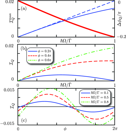
Figure 1: (Color online) (a) Charge-current amplitude $\mathcal{I}_{Q}^{\text{max}}$ (thin solid), its adiabatic approximation $\mathcal{I}_{Q}^{\text{max, ad}}$ (thin dashed), and phase shift $\Delta\phi_{Q}$ (thick) as a function of $\hbar\Omega/\bar{\Gamma}$. (b) Pumped current $\mathcal{I}_{Q}$ as a function of $\hbar\Omega/\bar{\Gamma}$, for $\phi=0.2\pi$ (solid), $\phi=0.4\pi$ (dashed), $\phi=0.6\pi$ (dash-dotted). (c) Pumped charge current $\mathcal{I}_{Q}$ as a function of $\phi$, for $\hbar\Omega/\Gamma=0.1$ (solid), $0.5$ (dashed) and $0.8$ (dash-dotted). All currents in units of $e\beta\Delta\Gamma_{L}\Delta\varepsilon/\hbar$. Other parameters: $\bar{\varepsilon}=k_{B}T\ln{2}$, $U=9\bar{\Gamma}$, $k_{B}T=3\bar{\Gamma}$, $p_{R}=0$, and $\bar{\gamma}_{R}=1/2$.

In the following, we concentrate on the peak at $\bar{\varepsilon}=k_{B}T\ln{2}$. In Fig. 1(a) the charge-current amplitude $\mathcal{I}_{Q}^{\text{max}}$ and the phase shift $\Delta\phi_{Q}$ are shown (solid lines) as a function of $\hbar\Omega/\bar{\Gamma}$. The amplitude is reduced as compared to the adiabatic approximation (dashed line). In Fig. 1(b) the pumped current $\mathcal{I}_{Q}$ is plotted as a function of the frequency $\Omega$ for different values of the pumping phase $\phi$. Deviations from the adiabatic approximation, simply given by the tangents at $\Omega=0$, become most pronounced as the pumping phase $\phi$ approaches zero: in this limit the phase shift $\Delta\phi_{Q}$, a striking signature of non-adiabatic pumping, is most important. Figure 1(c) shows $\mathcal{I}_{Q}$ as a function of the phase $\phi$ for different values of $\hbar\Omega/\bar{\Gamma}$. The growing relevance of the phase shift $\Delta\phi_{Q}$ as the pumping frequency is increased is apparent. As commented above, its most important consequence is the possibility to obtain an effective one-parameter pumping for $\phi=0,\pi$.

The frequency dependence of the phase shift $\Delta\phi_{Q}$ is that of a low–pass filter with cutoff frequency $\bar{\tau}_{Q}^{-1}$. It signals the reduced ability of fast pumps to transfer charge due to the non–zero response time of the dot to charge excitations, $\bar{\tau}_{Q}$.

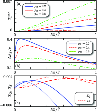
Figure 2: (Color online) (a) Spin-current amplitude $\mathcal{I}_{S}^{\text{max}}$ (thick) and its adiabatic approximation $\mathcal{I}_{S}^{\text{max,ad}}$ (thin) as a function of $\hbar\Omega/\bar{\Gamma}$ for different values of $p_{R}$. (b) Phase shift $\Delta\phi_{S}$ as a function of $\hbar\Omega/\bar{\Gamma}$ for different values of $p_{R}$.(c) Charge and spin currents $\mathcal{I}_{Q,S}$ as a function of $\hbar\Omega/\bar{\Gamma}$ with $p_{R}=0.4$ and $\phi=\pi/9$ for weak pumping (thick) and strong pumping (thin, with $\Delta\Gamma_{L}=\Delta\varepsilon=0.4\bar{\Gamma}$). Spin currents in units of $\beta\Delta\Gamma_{L}\Delta\varepsilon/2$. Other parameters: $\bar{\varepsilon}=k_{B}T\log{2}$, $U=9\bar{\Gamma}$, $k_{B}T=3\bar{\Gamma}$, and $\bar{\gamma}_{R}=1/2$.

Ferromagnetic case. In the weak-pumping regime for $p_{R}\neq 0$, we resort to a graphical presentation of the average pumped currents. In Fig. 2(a) and (b) the spin-current amplitude $\mathcal{I}_{S}^{\text{max}}$ and phase shift $\Delta\phi_{S}$ is shown as a function of the frequency $\Omega$. Both exhibit a strong dependence on the polarization $p_{R}$ of the ferromagnet. By contrast, the charge amplitude and phase shift (both not shown here) are almost insensitive to $p_{R}\neq 0$. In particular, $\Delta\phi_{Q}$ is essentially given by Eq. 11 and charge transfer is still dominated by the cutoff frequency $\bar{\tau}_{Q}^{-1}$. On the other hand, the intricate, coupled dynamics of spin and charge results in the spin phase being given by $\Delta\phi_{S}=\arctan(\Omega/2\Omega_{0})-\sum_{q=\pm}\arctan(\Omega/2\Omega_{q})$. For $\bar{\gamma}_{R}=1/2$, the cut-off frequencies are $\Omega_{0}=p_{R}^{2}\bar{\tau}_{S}^{-1}$ and $\Omega_{\pm}=\tau_{Q}^{-1}+\tau_{S}^{-1}\pm\sqrt{(\tau_{Q}^{-1}-\tau_{S}^{-1})^{2}+p_{R}^{2}(\bar{\tau}_{Q}\bar{\tau}_{S})^{-1}}$. The competition between $\Omega_{0}$ and the “hybridized” $\Omega_{\pm}$ gives rise to the non–monotonic behavior as well as the sign change of $\Delta\phi_{S}$. The most striking consequence of non–adiabaticity in the ferromagnetic case is the possibility to obtain a pure spin current, $\mathcal{I}_{S}\neq 0$ with $\mathcal{I}_{Q}=0$, by tuning $\Omega$ such that $\phi+\Delta\phi_{Q}(\Omega)=0$. This behavior is illustrated in Fig. 2(c), thick lines. The adiabatic approximation, missing the phase shifts, is unable to capture this effect. Pure spin pumping, as all the effects induced by the ferromagnetic lead, are enhanced for $\bar{\gamma}_{R}\to 1$.
We conclude discussing the experimental observability of the effects discussed above. Currents in the weak pumping regime are generally small. However, our theory is valid also for strong pumping where currents are larger and we have checked that all the results are not qualitatively modified. As an example, Fig. 2(c) (thin lines) shows the charge and spin currents for $\Delta\bar{\Gamma}_{L}=\Delta\varepsilon=0.4\bar{\Gamma}$. For a temperature $T$ of the order of 1 K ($k_{B}T\approx 90\mu$ eV) and $\bar{\Gamma}=k_{B}T/3$ , one has $e\beta\Delta\Gamma_{L}\Delta\varepsilon/\hbar\approx 500$ pA as the current unit. Clearly, pure spin pumping is still present. The charge current, ranging between -3 pA and 1 pA, is easily measurable. However, care needs to be exerted to minimize rectification effects due to stray capacitances and to distinguish them from pumping.
Conclusions. We have studied non-adiabatic two-parameter charge and spin pumping through an interacting quantum dot, tunnel coupled to metallic leads. In the sequential-tunneling regime, for frequencies smaller than the tunnel rates, all orders in the pumping frequency can be resummed exactly. We find frequency-dependent phase shifts for the pumped charge and spin current, neglected in the adiabatic approximation. They allow an effective single-parameter pumping, i.e., finite pumping currents when the two pumping parameters oscillate in phase or anti-phase. When one lead is ferromagnetic, the pumping frequency turns out to be an important parameter to control the spin current. In particular, due to the non-adiabaticity of pumping, pure spin currents can be generated. The effects discussed above can be experimentally verified in the strong-pumping regime, where the pumped currents are sizable.
Acknowledgements. We acknowledge financial support from the DFG via SPP 1285 and via SFB 491, and from INFM-CNR via Seed Project PLASE001.

References

- (1) H. Pothier et al., Europhys. Lett. 17, 249 (1992).
- (2) J.M. Martinis, M. Nahum, and H.D. Jensen, Phys. Rev. Lett. 72, 904 (1994); M.W. Keller et al., Appl. Phys. Lett. 69, 1804 (1996); R.L. Kautz, M.W. Keller, and J.M. Martinis, Phys. Rev. B 60, 8199 (1999).
- (3) M. Switkes et al., Science 283, 1905 (1999).
- (4) S. K. Watson, R. M. Potok, C. M. Marcus, and V. Umansky, Phys. Rev. Lett. 91, 258301 (2003).
- (5) N. E. Fletcher et al., Phys. Rev. B 68, 245310 (2003); J. Ebbecke et al., Appl. Phys. Lett. 84, 4319 (2004).
- (6) A. Fuhrer, C. Fasth, and L. Samuelson, Appl. Phys. Lett. 91, 052109 (2007).
- (7) M.R. Buitelaar et al., Phys. Rev. Lett. 101, 126803 (2008).
- (8) B. Kaestner et al., Appl. Phys. Lett. 92, 192106 (2008).
- (9) P. W. Brouwer, Phys. Rev. B 58, R10135 (1998).
- (10) F. Zhou, B. Spivak, and B. Altshuler, Phys. Rev. Lett. 82, 608 (1999).
- (11) M. Moskalets and M. Büttiker, Phys. Rev. B 64, 201305(R) (2001).
- (12) Y. Makhlin and A.D. Mirlin, Phys. Rev. Lett. 87, 276803 (2001).
- (13) M. Moskalets and M. Büttiker, Phys. Rev. B 66, 035306 (2002).
- (14) O. Entin-Wohlman, A. Aharony, and Y. Levinson, Phys. Rev. B 65, 195411 (2002).
- (15) I. L. Aleiner and A. V. Andreev, Phys. Rev. Lett. 81, 1286 (1998).
- (16) R. Citro, N. Andrei, and Q. Niu, Phys. Rev. B 68, 165312 (2003).
- (17) T. Aono, Phys. Rev. Lett. 93, 116601 (2004).
- (18) P. W. Brouwer, A. Lamacraft, and K. Flensberg, Phys. Rev. B 72, 075316 (2005).
- (19) J. Splettstoesser, M. Governale, J. König, and R. Fazio, Phys. Rev. Lett. 95, 246803 (2005).
- (20) E. Sela and Y. Oreg, Phys. Rev. Lett. 96, 166802 (2006).
- (21) J. Splettstoesser, M. Governale, J. König, and R. Fazio, Phys. Rev. B 74, 085305 (2006).
- (22) D. Fioretto and A. Silva, Phys. Rev. Lett. 100, 236803 (2008).
- (23) L. Arrachea, A. Levy Yeyati, and A. Martin-Rodero, Phys. Rev. B 77, 165326 (2008).
- (24) J. Splettstoesser, M. Governale, and J. König, Phys. Rev. B 77, 195320 (2008).
- (25) M. Moskalets and M. Büttiker, Phys. Rev. B 66, 205320 (2002); L. Arrachea and M. Moskalets, Phys. Rev. B 74, 245322 (2006); M. Moskalets and M. Büttiker, Phys. Rev. B 78, 035301 (2008).
- (26) B. L. Hazelzet, M. R. Wegewijs, T. H. Stoof, and Y. V. Nazarov, Phys. Rev. B 63, 165313 (2001).
- (27) E. Cota, R. Aguado, and G. Platero, Phys. Rev. Lett. 94, 107202 (2005); E. Cota, R. Aguado, and G. Platero, Phys. Rev. Lett. 94, 229901(E) (2005).
- (28) R. Sánchez, E. Cota, R. Aguado, and G. Platero, Phys. Rev. B 74 035326 (2006).
- (29) M. Braun and G. Burkard, Phys. Rev. Lett. 101, 036802 (2008).
- (30) C. Bruder and H. Schoeller, Phys. Rev. Lett. 72, 1076 (1994)
- (31) L. P. Kouwenhoven et al., Phys. Rev. Lett. 73, 3443 (1994); R. H. Blick et al., Appl. Phys. Lett. 67, 3924 (1995); H. Qin et al., Phys. Rev. B 63, 035320 (2001).
- (32) E. R. Mucciolo, C. Chamon, and C. M. Marcus, Phys. Rev. Lett. 89, 146802 (2002).
- (33) A. Walraff et al., Nature 431, 162 (2004).
- (34) R. Gommers, S. Bergamini, and F. Renzoni, Phys. Rev. Lett 95, 073003 (2005).
- (35) M. Grifoni and P. Hänggi, Phys. Rev. Lett. 76, 1611 (1996).
- (36) R.D. Astumian and I. Derenyi, Phys. Rev. Lett. 86, 3859 (2001).
- (37) F. Pistolesi and R. Fazio, Phys. Rev. Lett. 94, 036806 (2005).