Long-term stability of spotted regions and the activity-induced Rossiter-McLaughlin effect on V889 Herculis

Abstract

Context. The young active G-dwarf star V889 Herculis (HD 171488) shows pronounced spots in Doppler images as well as large variations in photometry and radial velocity (RV) measurements. However, the lifetime and evolution of its active regions are not well known.

Aims. We study the existence and stability of active regions on the star’s surface using complementary data and methods. Furthermore, we analyze the correlation of spot-induced RV variations and Doppler images.

Methods. Photometry and high-resolution spectroscopy are used to examine stellar activity. A CLEAN-like Doppler Imaging (DI) algorithm is used to derive surface reconstructions. We study high-precision RV curves to determine their modulation due to stellar activity in analogy to the Rossiter-McLaughlin effect. To this end we develop a measure for the shift of a line’s center and compare it to RV measurements.

Results. We show that large spotted regions exist on V889 Her for more than one year remaining similar in their large scale structure and position. This applies to several time periods of our observations, which cover more than a decade. Furthermore we use DI line profile reconstructions to identify influences of long-lasting starspots on RV measurements. In this way we verify the RV curve’s agreement with our Doppler images. Based on long-term RV data we confirm V889 Her’s rotation period of $1.3371\,\pm\,0.0002$ days.

1 Introduction

The Sun is the only star which is sufficiently close to resolve surface inhomogeneities in detail. Most prominent among them are sunspots. At solar maximum they cover approximately $0.3\,-\,0.4$ % of the total solar surface (Solanki & Unruh, 2004) and individual sunspots reach diameters of roughly $2$ degrees (Schrijver, 2002) on average. Two examples of exceptionally large spots on the Sun were observed in March 1947 (Willis & Tulunay, 1979), covering about $0.6$ % of the solar disk, and on March 29, 2001 (Kosovichev et al., 2001), with a size of more than $0.35$ % of the visible surface. The appearance and movement of sunspots is often displayed in ‘butterfly diagrams’ which show that their positions are confined to a band of $\pm\,30\,-\,40$ degrees above and below the equator (e.g. Li et al. 2001). Their lifetimes vary from a few days to several weeks ($\apprle$ month) and appear to be related to the spot-size, larger spots persist longer (Petrovay & van Driel-Gesztelyi, 1997).

This picture seems to be different in several respects from other stars of similar spectral type, although these observations are biased towards stars with small rotation periods, which is a basic requirement of the currently available techniques to study stellar surface inhomogeneities. Contrary to the slowly rotating Sun we observe that many rapid rotators ($v\sin(i)\,\apprge\,25$ km/s) possess large areas covered with features of significantly lower temperatures. One of the most extreme examples was found in the binary system VW Cep with a surface coverage of $\sim\,70$ % (Hendry & Mochnacki, 2000). Starspots or spot groups with sizes of several dozens of degrees have been detected not only at low and intermediate latitudes, but also covering the polar regions. These polar spots form long-lasting features, sometimes persisting over years or possibly even decades (Vogt et al., 1999; Jeffers et al., 2007). The limits of current techniques often prevent us from discerning large monolithic spots from groups of individual spots within an active region. Whatever their detailed nature, these structures have much longer lifetimes than sunspots. Large spotted regions have been monitored on some stars for years showing only small changes (e.g. Korhonen et al. 2007 and Lanza et al. 2006), although individual starspots appear to evolve on timescales of several weeks (Barnes et al., 1998; Wolter et al., 2005).

Such observations gave rise to the idea of ‘active longitudes’; regions on the stellar surface that persist in their large scale structure (Korhonen et al., 2001). The term ‘active longitudes’ may partially reflect the weakness of surface reconstruction methods to resolve the positions of stellar features in longitude more accurately than in latitude. Such regions show a high spot coverage stretching over a large area of the star, persisting for many months or years, which translates into several hundreds of stellar rotations. It is largely unknown whether their internal structure is variable, i.e., to what degree spots move, disappear, or form inside of them. However, in some cases their global structure remains stable over large time periods (e.g. Berdyugina & Järvinen 2005).

In this paper we show that large spotted regions on V889’s surface persist on time scales of hundreds of days. To this end we use photometric data, Doppler images, and radial velocity (RV) measurements. Section 2 summarizes characteristics of the star and its surface features. In Sect. 3 we present observational characteristics of the Hipparcos data, the Doppler Imaging (DI) data, and the RV measurements. Section 4 explains the process of the lightcurve analysis, while Sects. 5 and 6 contain the analysis of the RV measurements and the DI process. Section 7 gives a discussion on all data sets and their correlation, followed by a summary of the main results in Sect. 8. Finally, the appendix covers mathematical aspects of the equation used to calculate RV shifts from line profiles, and contains all DI line profile reconstructions.

2 Object

Table 1: Stellar parameters of V889 Her

Parameter	Value
Spectral type	G0V
Distance (Hipparcos)	$37.2\pm 1.2$ pc
$M_{\mathrm{hipp,\,mean}}$	$7\aas@@fstack{m}523\,\pm\,0\aas@@fstack{m}004$
$M_{\mathrm{hipp,\,max}}$	$7\aas@@fstack{m}48\,\pm\,0\aas@@fstack{m}01$
$M_{\mathrm{hipp,\,min}}$	$7\aas@@fstack{m}57\,\pm\,0\aas@@fstack{m}01$
$V_{\mathrm{max}}$	$7\aas@@fstack{m}34$
$v\sin(i)^{f}$	$39.0\pm 0.5\ \mathrm{km}\,\mathrm{s}^{-1}$
Rotation periodf	$1.3371\pm 0.0002$ d
Inclination $i$ f	$\sim\,55$°

The fast-rotating solar analog V889 Herculis (HD 171488) has been a subject of astrophysical studies for many years. Its good visibility from the northern hemisphere, large brightness, pronounced photometric variability, and high rotation velocity make it an interesting target. Especially its rotation period of $1.3$ days is convenient to study the lifetimes of atmospheric structures, since observations covering four consecutive nights offer a complete coverage of all rotation phases. Therefore, it is a well-suited candidate for DI and other studies of stellar activity. Doppler images of V889 Her were published by Strassmeier et al. (2003) and Marsden et al. (2006). Some of its basic properties are summarized in Table 1.

Surface reconstructions of V889 Her from these authors reveal a large polar spot that changes in size and structure but has yet always been present. Additionally, all published Doppler images show some medium- and low-latitude spots which may stretch over a few dozens of degrees and, thus, cover a significant fraction of the stellar surface. Strassmeier et al. (2003) present surface maps dominated by an asymmetric polar spot with a temperature difference of $\Delta T\,\approx\,1\,600$ K to the unspotted surface at $\approx\,5\,900$ K. Several low-latitude spots are resolved as well with $\Delta T\,\approx\,500-800$ K. Strassmeier et al. determine a rotation period of $P\,=\,1.3371\,\pm\,0.0002$ days using long-term photometry. Marsden et al. (2006) reconstruct a polar spot of similar size down to almost +60° in latitude and two pronounced low-latitude spots at +30°. Additionally reconstructions for the magnetic field topology were possible by Zeeman Doppler Imaging (ZDI), which yield only weak signs of a polar spot (in agreement with ZDI images of other objects, see e.g. Donati et al. 2003) and confirm the low-latitude features. Marsden et al. (2006) find a different rotation period of $P\,=\,1.313\,\pm\,0.004$ days and a differential rotation of $\alpha\,=\,\Delta P/P\,=\,0.08$, while for the Sun a value of $\alpha\,\approx\,0.2\,-\,0.3$ is measured. $\Delta P$ denotes the difference between the equatorial and the polar rotation period.

Up to now it has not been known on which time scales spotted regions on the surface of V889 Her form and dissolve and how heavily the effects of differential rotation and meridional flows influence their development in shape and position. All surface features are presumably in constant evolution, but there are indications in previous Doppler images and reconstructions in this paper that especially large active regions besides the polar spot may have fixed positions and high stability. Evidence of such preferred longitudes was detected before in other stars (e.g. Berdyugina 2007), while Barnes et al. (1998) do not find long-lived spots on rapidly rotating G dwarfs indicating that this is not a general characteristic for this type of stars.

3 Observations

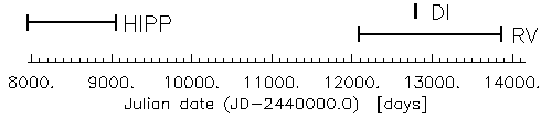
Figure 1: Time coverage of observations used in this paper. HIPP represents the Hipparcos, DI the Doppler Imaging, and RV the radial velocity data sets.

We use three different kinds of data sets to determine the stability of spotted regions on V889 Her: long-term photometric observations from the Hipparcos mission, and two different time series of high-resolution spectra used for radial velocity (RV) measurements and Doppler Imaging. The short-term time series suitable for DI yield snapshots of the spot distribution, which we correlate with our long-term RV measurements covering the same time period. Figure 1 visualizes the time coverage of the three data sets used in this work.

3.1 Hipparcos data

The Hipparcos satellite obtained a lightcurve of V889 Her during its 3.3 years mission. The available data cover the time between March 1990 and March 1993 with about 150 unevenly sampled photometric data points (Perryman et al., 1997).

3.2 RV measurements

The RV observations were carried out at the 2 m Alfred Jensch Telescope at the Thüringer Landessternwarte in Tautenburg, Germany. It is equipped with a Coudé Echelle spectrograph, which provides a resolving power of $R=67\,000$ and a wavelength range of $4\,700$ - $7\,400$ Å. In total, $62$ radial velocity shifts were analyzed in this paper. For the purpose of a stable wavelength calibration, an iodine cell was used (Marcy & Butler, 1992); for more information about the spectrograph see Hatzes et al. (2005).

The exposure times vary between 15 and 20 minutes, the typical signal-to-noise ratio is 70. The data was reduced with the Image Reduction and Analysis Facility (IRAF, Tody 1993). For the RV measurements the spectral range between $5\,000$ Å and $6\,300$ Å is split up into about 130 pieces (‘chunks’). RV shifts are determined independently for each wavelength piece, the mean of all pieces yields the radial velocity with its error given as the standard deviation.

For the analysis, the RV curves are split up into shorter subintervals. Their exact definitions and an overview of the entire observations are given in Fig. 6.

3.3 Doppler Imaging spectra

The time series of high-resolution spectra used for Doppler Imaging was observed in June 2003 at the Nordic Optical Telescope (NOT) on La Palma. A total of 61 spectra of V889 Her were obtained with the SOFIN Echelle spectrograph mounted at the Cassegrain focus of the 2.56 m telescope, covering several preselected spectral regions between $3\,750$ Å and $11\,300$ Å with a width of e.g. 60 Å per region around 6000 Å. The average signal-to-noise ratio of these spectra is above 150. The chosen slit width of 65 $\mu$ provides a nominal resolving power of $76\,000$. The data cover 8 nights (2 blocks of 4 consecutive nights), i.e., two full rotations of the star, with a homogeneous phase coverage. Approximately 3 rotations of the star lie between the two obtained Doppler images. The average exposure time for these observations was 20 minutes. A short summary of the observation dates and the number of spectra is given in Table 2.

The Echelle spectra were reduced with the software package described in Ilyin (2000), performing bias subtraction, master flat field correction, scattered light modeling with bi-cubic splines, and optimum extraction of spectra including cosmic spikes rejection. Blaze correction and CCD fringe removal was accomplished using flat field exposures that were reduced in a similar way. The wavelength calibration is based on two Th-Ar spectra taken before and after each object exposure.

Table 2: Nordic Optical Telescope data

N	Observation dates	Julian date	Total	Used
1 - 4	June 09, 2003	3799.54	42	39
	June 12, 2003	3802.75
9 - 12	June 16, 2003	3807.47	19	19
	June 20, 2003	3810.69

4 Lightcurve analysis

4.1 Our modeling approach

Lightcurve modeling has a long-standing history in astronomy. An overview on its history as well as on different approaches towards a solution of this problem can for instance be found in Eker (1994).

The Hipparcos data are of limited accuracy and rather inhomogeneously sampled in time. Therefore, we revert to a simple but robust modeling approach. We subdivide the star into homogeneously spaced longitude intervals, and assume that these areas are homogeneously covered by spots. In the fitting process the relative brightness (spot coverage) of these strips is then varied until the observed lightcurve is matched optimally. We apply two different fit procedures: Either we allow fits restricted by a specific assumption about the number of active regions on the stellar surface; in this case every active region is modeled by a longitudinal Gaussian brightness distribution. Or, alternatively, a ‘free’ fit can be carried out, where all surface elements are varied independently.

Note that each individual longitude interval produces the same lightcurve profile (normalized by its intensity, i.e. spot coverage), phase shifted according to its position on the surface. The resulting lightcurve is a linear superposition of the individual contributions. When we use a relatively low number of longitude intervals (say $10$), it is quite obvious that the contributions are linearly independent (given a non pole-on view), and the superposition is uniquely defined. Working with real data, measurement errors and phase coverage limit the uniqueness of the reconstruction; nevertheless, with a low number of longitude intervals, only neighboring intervals show considerable dependence.

In either case latitudinal information is not recovered, which $-$ given the data quality and sampling $-$ would be an ambitious task anyway.

4.2 Lifetime analysis of structures imprinted on the Hipparcos lightcurve

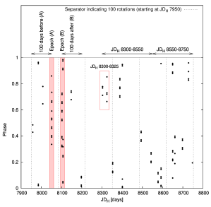
Figure 2: Time vs. phase diagram (period$\,=\,1.3371$ days) for the Hipparcos measurements (represented by points). Periods covering $100$ rotations are indicated by vertical, dotted lines. Time and phase intervals of special interest are marked by arrows and boxes; see text for more details.

As demonstrated in Fig. 2, the sampling of the Hipparcos lightcurve is inhomogeneous so that the data contain quite a number of isolated measurements. Fortunately, there are some observation epochs with much better phase coverage. The first one (A) can be found at $\mathrm{JD}_{H}$ $\approx\,8050$ where we find $12$ data points observed during about a day, and the second one (B) is found about $50$ days later containing $22$ measurements distributed over $5$ days (cf. Fig. 2). The corresponding data points are shown in the upper panel of Fig. 3, where we also present lightcurve reconstructions obtained under the assumption of a single active region on the stellar surface. The measurements originating from epoch (A) cover only phases $0.3\,-\,0.9$, whereas epoch (B) provides nearly full phase coverage. Clearly, the minimum in interval (A) is sharper than in (B) and also displaced in phase by about $0.1$ corresponding to a longitude shift of $\approx 36$° for the activity center. While this shows that there is significant evolution of the lightcurve within $50$ days, the lightcurve also maintains its overall appearance showing a pronounced minimum at about $120$° longitude as the most distinct feature. The differences between the two epochs can be caused by evolution of the stellar surface and/or by an inappropriate lightcurve folding due to an incorrect rotation period. According to Marsden et al. (2006), V889 Her shows strong differential rotation making its period a function of latitude; folding the data with a period inconsistent with the location of the active regions could mimic surface evolution. Note that adopting a rotation period of $1.3371\,\pm\,0.0002$ days, as given by Strassmeier et al. (2003), the relative phase error between two data points separated by $100$ rotations is only $\approx\,1.5$ % so that we can neglect this as an error source here.

In an effort to check how the locations of other, more distant data points compare to the lightcurves obtained during epochs (A) and (B), we combine the two data sets and fit the result using the ‘free’ fit approach with $9$ (independent) surface elements (Fig. 3, lower panel). Considering the evolution between epochs (A) and (B), the thus obtained results are of course time averages rather than snapshots. The fit provides evidence for a pronounced active region at a longitude of about $120$° and another less pronounced structure at about $240$°.

Now we check statistically whether it is justified to assume that the time averaged model at hand remains an appropriate approximation of the lightcurve over a longer time span (given a period of $1.3371$ d). Within about one hundred days ($\approx\,75$ rotations) before epoch (A) (measurements in $\mathrm{JD}_{H}\,=\,7950\,-\,8010$) there are $3$ other observation periods providing $8$ additional data points and within about the same time span after epoch (B) (measurements in $\mathrm{JD}_{H}\,=\,8145\,-\,8200$) another $7$ measurements are distributed over two observation epochs (see Fig. 2). In the middle panel of Fig. 3 we show the same model lightcurve as before as well as the $15$ additional data points (triangles and filled circles). Apparently, the model provides an acceptable description of the observations. Formally, we expect a $\chi^{2}$ value of $15\,\pm\,5.5$ for $15$ data points drawn from the same model; the shown model yields $21.2$ with about one third of it contributed by a single data point.

If the lightcurve evolves fast with respect to the time span under consideration, we expect the data points to be distributed randomly, and in the following we assume that the lightcurve amplitude observed in epochs (A) and (B) remains representative. From a Monte Carlo simulation we then estimate that the probability to obtain a value of $21.2$ or less for $\chi^{2}$ from the same number of data points uniformly distributed over the lightcurve amplitude is $\approx\,2.5$ %. During the simulation we do not vary the data points in phase and all data points enclosed by a single observation epoch are regarded as dependent and, therefore, are varied as a single unit.

We conclude that the Hipparcos lightcurve is compatible with a rotation period of $1.3371$ d and a surface configuration dominated by an active region at a longitude of about $120$° for at least $50$ days and probably up to about $200$ days. We, however, caution the reader that the data do not allow to exclude other scenarios.

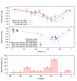
Figure 3: Upper panel: The data and models for observation epoch (A) (squares) and (B) (circles). The dotted and dashed lines indicate model fits obtained for epoch (A) and (B) assuming a surface dominated by one active region, respectively. The solid line constitutes a model based on the combined data of epoch (A) and (B). Middle panel: The ‘combined’ model from the upper panel as a solid line as well as additional data points observed before and after epochs (A) and (B). Lower panel: The spot filling factor obtained from longitude reconstruction. The spot-photosphere contrast was assumed to be $50$ %. (Note that the error bars do not take into account mutual dependencies of the bins.)

The middle panel of Fig. 3 includes measurements carried out during the $\mathrm{JD}_{H}\,\approx\,8300\,-\,8325$ time interval (open circles in Fig. 3, also marked in Fig. 2) about $210$ days after those of epoch (B). The associated data points confirm the presence of a minimum at about the same position during this period, although their phase coverage is poor. Unfortunately, phase coverage remains a problem throughout the analysis of the entire rest of the Hipparcos data set. Even if we combine the data obtained during the following $\approx\,450$ days ($\mathrm{JD}_{H}\,=\,8300\,-\,8750$), a (connected) phase interval covering about $30$ % of the lightcurve remains unobserved (see Fig. 2). Furthermore, the measurements are distributed very inhomogeneously in time providing no further well covered individual epochs forcing us to consider longer time spans.

In the upper panel of Fig. 4 we show the data pertaining to the $\mathrm{JD}_{H}\,=\,8300\,-\,8550$ time interval as well as a ‘free’ model fit obtained from them; note that this covers some data points already shown in the middle panel of Fig. 3. Additionally, we show the lightcurve obtained from combining epochs (A) and (B) (dashed line). As already indicated earlier, both lightcurves bear considerable resemblance at phases $\geq\,0.5$. This does no longer hold for phases $\leq\,0.5$, where the data clearly indicate the presence of a second pronounced minimum caused by an active region at a longitude of about $280$°. While this stellar region considerably increased its impact on the lightcurve compared to the previous data, the one at a longitude of $\approx 120$°$-$ although still existing $-$ is less significant and may be in a process of disintegration.

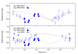
Figure 4: Upper panel: Measurements between $\mathrm{JD}_{H}\,=\,8300$ and $8550$. The dashed lines indicate the model obtained from the combined epochs (A) and (B), the solid lines show the lightcurve obtained from the given intervals. Lower panel: Data of the $\mathrm{JD}_{H}\,=\,8490\,-\,8750$ time interval and $5$ additional points from $\mathrm{JD}_{H}\,=\,9055$.

During the next $\approx\,160$ days (see Fig. 4, lower panel), there is a clear evolution in the shape of the lightcurve, potentially indicating evolution of the newly emerged active region. Unfortunately, the phase interval sampling of the lower longitude active region is very poor, so we can no longer trace its evolution. The measurements presented in this panel show a trend indicating an $\approx\,0.05$ mag brightening of V889 Her, which may be related to a periodic sinusoidal long-term trend with about the right amplitude and a period of $\approx\,2600$ days detected by Strassmeier et al. (2003).

Even though a stellar surface with two dominating active regions evolving in time as indicated by the panels of Fig. 4 seems physically reasonable, we caution that the time span covered here is $450$ days, which is twice as long as the time span considered in Fig. 3 and, in particular, $9$ times longer than the separation between epochs (A) and (B). Therefore, a variation of the rotation period in the percent-regime already has considerable impact on the lightcurves.

Throughout the above analysis our models yield a spot coverage fraction of $\approx\,10$ % assuming a spot-photosphere brightness-contrast of $1/2$. Only during the last observation epochs ($\mathrm{JD}_{H}\,>\,8550$) the model provides a lower fraction of $\approx\,6$ %, which may, however, also be related to the poor phase coverage obtained in this time span.

5 Radial velocity measurements

5.1 Activity-related radial velocity measurements

Stellar activity influences the strength and profiles of spectral lines and can, therefore, affect RV measurements, whose precision hinges on symmetric and narrow lines. For example, a spot located on the hemisphere of the star rotating towards the observer diminishes the amount of light contributing to the blue-shifted line wing, leading to an asymmetric line shape. This is not crucial for slowly rotating stars as long as their spectral lines are predominantly broadened by thermal and other mechanisms instead of rotation. Locally restricted surface features only become detectable in very broad lines where the spectra are sufficiently oversampled. In general, slow rotators should be less active showing fewer and smaller spots, and rotational broadening is less important for their line profiles. For fast rotators with $v\sin(i)\apprge 25$ km/s, where all spectral lines are dominantly broadened by the Doppler effect, such surface features become resolvable in the stellar spectrum.

This is one reason why high accuracy RV measurements are difficult for rapidly rotating stars. Stellar activity can deform their line profiles and, using standard RV detection methods, these deformations lead to RV shifts due to asymmetric and variable line shapes. RV shifts induced by stellar activity can be of the order of several 100 m/s for stars with $v\sin(i)\,\apprge\,5$ km/s (Saar & Donahue 1997 and Saar et al. 1998), and even higher for larger rotation velocities, i.e., up to a factor of thousand higher than the state-of-the-art RV precision. While this is a nuisance for companion detections around highly active stars, it can be used as an additional source of information regarding the localization of atmospheric features. RV modulations due to activity can be seen as an activity-induced Rossiter-McLaughlin effect (Ohta et al., 2005) otherwise used for planet detection and characterization: an isolated spot on a stellar surface causes a variation of the RV curve very similar to the one caused by a transiting planet.

Nevertheless, it is a different situation with spots when using the Rossiter-McLaughlin effect. On the one hand it is simpler, if the spot distribution does not change too rapidly, because one usually knows the rotation period of a spotted star and has a chance to observe many spot transits on small time scales for low rotation periods. On the other hand it is more complicated because stellar spot distributions can change on short time scales and, generally, surfaces of active stars are populated by more than only one spot, which means that one measures a superposition of Rossiter-McLaughlin effects for all visible spots. As a result, RV curves modulated by stellar activity generally do not look like the curves derived from planetary transits. They may have complicated structures instead, which cannot be identified as obvious superpositions of Rossiter-McLaughlin effects. However, it is possible to detect an activity-induced effect for simple configurations of spot distributions, as demonstrated in this paper.

5.2 Rotation period

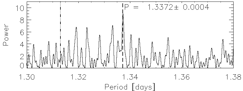
Figure 5: Periodogram of the RV data on the interval relevant for V889 Her’s rotation period. The period determined from the highest peak is given in the figure; Marsden et al.’s value of $1.313$ d is marked by the dash-dotted line. See Sect. 5.2 for details.

The interpretation of long-term observations requires a precise stellar rotation period. Data sets stretching over periods of months or years must be folded back at a well-known phase scale to be able to detect any long-term stability. In the case of V889 Her this is possible on the basis of extensive photometric observations yielding a rotation period of $P\,=\,1.3371\,\pm\,0.0002$ days (Strassmeier et al., 2003). Note that we obtain the same value from a periodogram of our RV measurements, presented in Fig. 5, where the most significant peak in the relevant period interval is located at $P\,=\,1.3372\,\pm\,0.0004$ days.

The position of Marsden et al.’s rotation period is marked as well in Fig. 5; clearly, our RV data support the period determined by Strassmeier et al., which we use in the following. This rotation period applies to the case of rigid rotation; since no significant evidence for differential rotation was found in our data sets, we hold on to the simple model (see Sect. 7).

Given Strassmeier et al.’s error of the rotation period $\Delta P\,=\,0.0002$ days and considering an acceptable phase error of $\Delta\phi\,=\,0.05$ (translating into $\approx\,20$°), we can calculate the time span $\Delta\mathrm{JD}$ that can be phase-folded with the required accuracy. The selected maximum phase error is consistent with longitude accuracies of $\apprle\,\pm\,10$° achieved during the modeling of large active regions in the Hipparcos photometry. We use equation

$$\Delta\mathrm{JD}\ =\ \left|\left(\frac{1}{P+\Delta P}-\frac{1}{P}\right)^{-1}\cdot\Delta\phi\right|\ ,$$ (1)

derived from $\phi+\Delta\phi\,=\,\Delta\mathrm{JD}/(P+\Delta P)$, to determine a maximum duration of $\Delta\mathrm{JD}\ \approx\ 450$ days for which we can trace a structure in the lightcurve with a phase accuracy better than $0.05$.

We use $\mathrm{JD}_{0}\,=\,2449000.0$ to calculate the phases $\phi$ from

$$\phi=\frac{\mathrm{JD}\ -\ \mathrm{JD}_{0}}{P_{rot}}\ .$$ (2)

Stellar surface coordinates are defined consistently for all surface maps (see e.g. Fig. 7). Rotation phases are calculated for surfaces rotating towards decreasing longitudes, which means that a phase $\phi$ can be translated into a longitude $l$ using the equation $\phi\ =\ (360^{\circ}-l)/360^{\circ}$.

   

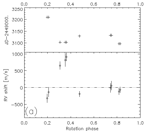
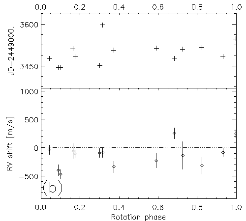
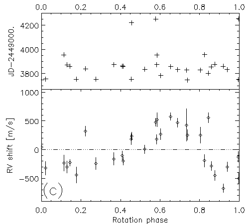
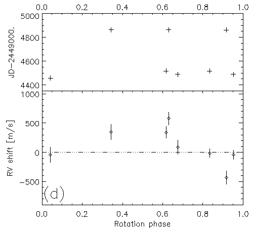
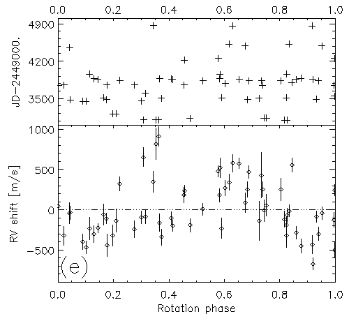
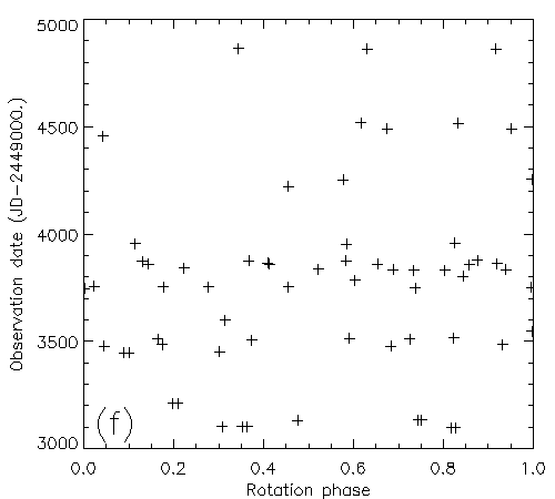
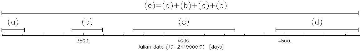
Figure 6: Radial velocity measurements of V889 Her. The data set was separated into several parts to visualize the stability of structures in the RV curve. Each interval of a few hundred days shows characteristic influences of the star’s activity on the spectra causing RV shifts. Large spotted regions are visible in the RV curves for more than a hundred days before they finally dissolve or significantly change positions. Panel (f) shows phase coverage of the entire data set.

5.3 Detection of stable active regions in the RV curves

The RV measurements of V889 Her cover a time period of almost $2\,000$ days, which translates into approximately $1\,500$ stellar rotations. The distribution of data points over the entire observations is given in Fig. 6 panel (f); in panels (a) to (e) we subdivide the data into shorter intervals. The lower panel illustrates the time coverage of each panel.

The modulation of the RV curve does not reveal any stellar companion or extrasolar planet within the limits of its accuracy. There are large quasi-periodic variations in the curve changing on large time scales of several months, which is not consistent with a low-mass companion. The average accuracy per data point is about $150$ m/s.

Nevertheless, we do detect periodicity in the RV curve of Fig. 6. The periodogram of the data shows a high peak at the star’s rotation period (cf. Sect. 5.2), which suggests that the modulation of the curve is related to its activity. In Fig. 6 subintervals of the RV data are presented, where the global shape of the curve does not change significantly; however, between the panels substantial changes of the RV curve take place. Panel (c) contains a large fraction of all data points (almost 50 %) and clearly shows a stable modulation of the RV curve with rotation for a duration of at least $\apprge\,150$ days ($\mathrm{JD}\,=\,3750\,-\,3900$); this time span may even be longer since neighboring points from $\mathrm{JD}\,\approx\,3950$ and $\approx\,4250$ support the curve as well.

The RV modulation visible in panel (c) dominates the RV curve over the entire time interval, as visible in panel (e) where the phase-folded RV curve of all data points is presented. This is the reason why the periodogram returns the star’s exact rotation period, although the spot distribution changes on long time scales. It may not be possible to obtain the rotation period from periodograms of RV curves for a faster changing spot distribution. Its effects on the RV curve will shift in phase and change in amplitude, which is not compensated by regular periodogram algorithms. If the rotation period is known and a sufficiently high phase coverage is available, the data can be subdivided into intervals with stable RV modulations associated to stable global spot distributions.

It is difficult to detect activity-induced Rossiter-McLaughlin effects (see Sect. 5.1) in the other panels of Fig. 6 due to the poorer data sampling. Panel (a) possibly contains some evidence for such a structure but further complementary data, i.e., Doppler images or lightcurves, are necessary to confirm this assumption. Panel (b) does not show any modulation implying that the spot distribution of panel (c) must have formed (or strongly intensified) after $\mathrm{JD}\,\approx\,3500$. There are possibly some signatures of this modulation left in panel (d); the rather poor phase coverage makes it hard to determine to which degree the spot distribution changed.

6 Doppler Imaging

Surface inhomogeneities cause deformations of spectral line profiles which can be used to reconstruct the spot distribution. This is achieved by Doppler Imaging (Vogt & Penrod, 1983). DI is limited to fast rotating stars where the broadening of the spectral lines is dominated by rotational broadening. Given the rotation velocity and period of V889 Her, surface reconstructions of this star can be achieved (cf. Strassmeier et al., 2003; Marsden et al., 2006).

6.1 CLEAN-like Doppler Imaging algorithm

For Doppler Imaging (DI) we use the CLEAN-like algorithm ‘CLDI’ (Wolter, 2004; Wolter et al., 2005). Starting with a ‘standard’ line profile adopted for the unspotted star, the program deforms the line profiles using an iteratively constructed stellar surface in order to match the shape of the spectral lines for all observed phases. This is done using ‘probability maps’ that show regions of tentative spot locations (Kürster, 1993). These maps do not give a probability in a strict statistical sense, instead they are ‘backprojections’ of the derivations between the observed and reconstructed line profiles onto the stellar surface. Spots are set at the most intense surface element of these backprojections as long as the deviations between the observed and reconstructed line profiles keep decreasing.

Several parameters must be supplied a priori to the DI process: the rotation period $P$, the projected rotation velocity $v\sin(i)$, the stellar inclination $i$, and the linear limb darkening parameter $\epsilon$ (with $I_{C}/I^{0}_{C}\,=\,1-\epsilon+\epsilon\cos\Theta$ where $\cos\Theta$ is the projected distance from the center of the stellar disk in units of the stellar radius (Gray, 1992)). Table 4 contains the values of these parameters adopted for our DI, additional stellar properties are given in Table 1, while Tab. 3 lists the lines used for the surface reconstructions.

The Doppler maps are reconstructed in terms of a spot filling factor between $0$ (no spot) and $1$ (completely spotted) where the number of possible graduations $n_{T}\,\geq\,2$ must be preselected. Spotted surface elements are areas with lower continuum intensity than the unspotted stellar surface, CLDI does not explicitly determine spot temperatures. We find no differential rotation within our detection limits; reliable small-scale structures close to the pole are hardly resolved preventing the determination of a polar rotation period (see Fig. 7). Reconstructions of the star taken several rotation periods apart do not yield significant identifications of systematically shifted features (see Appendix Fig. 10 for cross-correlation maps). Doppler images calculated using Marsden et al.’s differential rotation law do not improve $\chi^{2}$. Therefore, we refrain from modifying the rigid rotation law used in our reconstructions. The limb darkening parameter was adjusted for each line to obtain an optimal fit of the standard line profile to the observed lines, resulting in values between $\epsilon\ =\ 0.6$ and $0.8$.

Based on a comparison of our reconstructions from different spectral lines (Fig. 7), we estimate their surface resolution as approximately $10$° corresponding to $2\times 2$ surface elements; a few features are poorer localized in latitude (e.g. feature C in the left column maps of Fig. 7). Isolated surface elements are not reliably localized, they are an artifact of the CLDI algorithm due to noise and/or short-term spot evolution on small spatial scales.

The estimated reduced $\chi^{2}$ values of our reconstructions, averaged over all phases, are between $0.3$ and $1.5$. It is not possible to provide a strictly reduced $\chi^{2}$, since the number of parameters is not known in the CLEAN-like approach; however, the values are close to $1$ and the reconstruction show good agreement with the line profiles (see Appendix 11).

6.2 Doppler Imaging of V889 Her

	Nights 1 - 4	Nights 9 - 12
6122 Å
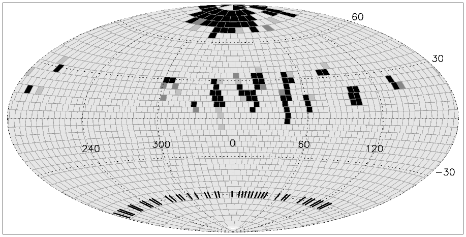
6439 Å

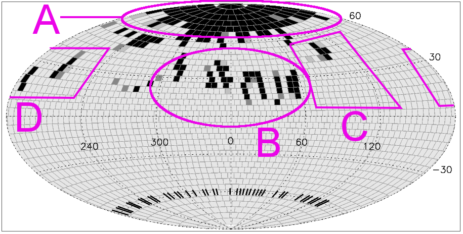
Figure 7: Doppler images of V889 Her, each observed during three stellar rotations. The images in the left column are separated from the right ones by three rotations. Each row contains images reconstructed from the indicated spectral line. Ticks in the southern hemispheres indicate the observed phases used for the reconstruction. Letters A$-$D annotate spot regions that can be commonly identified in several reconstructions. See Sects. 6.1 and 7 for discussion.

Table 3: Absorption lines used for Doppler Imaging.

Name	Rest wavelength (Å)	Chemical element
6122	6122.22	Ca I
6439	6439.08	Ca I

Figure 7 shows four reconstructed Doppler images of V889 Her. The left column contains the images of the first full rotation, based on spectra of four consecutive nights (‘nights $1\,-\,4$’), i.e. three stellar rotations. The right column shows images of the second full rotation (‘nights $9\,-\,12$’), also taken during three consecutive stellar rotations. Three stellar rotations remained unobserved between the images of the two columns. Table 3 contains details of the lines used for DI.

The left column maps are based on 39 observed rotation phases, quite evenly distributed apart from a gap ranging from about 130° to 180° in surface longitude, while the right column maps are based on 19 phases. The left 6439 Å-map labels the spot regions A$\,-\,$D, that can be commonly identified in several reconstructions. In agreement with previous reconstructions of V889 Her, all our maps show a large polar spot. Causing almost no rotational modulation, the reconstructed size of a polar spot depends sensitively on the adopted line parameters. However, keeping these uncertainties in mind, two properties of the polar spot are reliably found in our reconstructions: it extends down to a latitude of approximately +60° and it apparently exhibits a weak asymmetry, being slightly more pronounced on the 0$\,-\,$180° hemisphere (right half of each map in Fig. 7).

Table 4: Reconstruction parameters adopted for DI.

Parameter	Value
Differential rotation $\alpha$	0.
Limb darkening $\epsilon$	$0.6\,-\,0.8$
Macro-turbulence	2 / 12 $\mathrm{km}\,\mathrm{s}^{-1}$
Contrast photosphere/spot	0.5
$n_{T}$	4

Both the dominant low-latitude feature B and its much smaller companion C persist through all 9 rotations covered by our Doppler maps. They show little distinct evolution apart from a slightly more pronounced gap in the middle of feature B during nights $9\,-\,12$. The other low-latitude feature (D) dissolves between the two observed sequences.

When interpreting Doppler images, one must keep in mind that spots located on the southern hemisphere are largely projected onto the northern hemisphere. Therefore, all given spot latitudes have an unspecified sign. Additionally, surface features based on poor phase coverage have a higher uncertainty and must be judged with care. The latter aspect does not apply to any of the features discussed above.

We conclude that all maps show large spotted regions on poles and low latitudes. Although these features (A $-$ D) seem to be subject to evolution, their change in fine structure is significantly affected by reconstruction uncertainties. However, some spot groups are similar in their large scale structure, especially region B which keeps its character as ‘dominant feature’ during the observations; this is also visible in the lightcurves and RV-curves of Fig. 8. Within our accuracy limits we do not find evidence of differential rotation: the identified low-latitude surface features do not show a systematic shift in longitude during the observed 9 rotations. Neither does the polar spot or its lower-latitude appendices exhibit well-defined asymmetries which would be required to measure a differing rotation period for higher latitudes. This justifies our choice of a rigid rotation for the surface reconstruction in agreement with (Strassmeier et al., 2003). To obtain significant measurements of V889 Her’s differential rotation, considerably less noisy line profiles would be required as input of the DI.

Measured RV curve
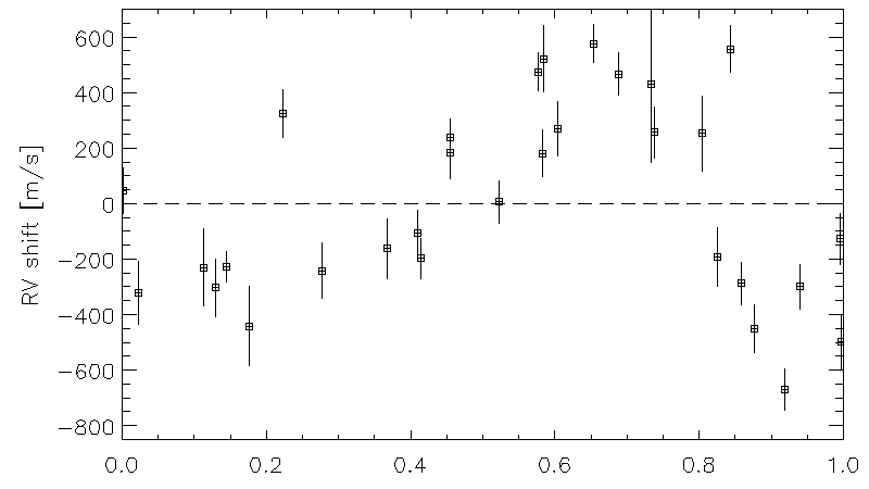
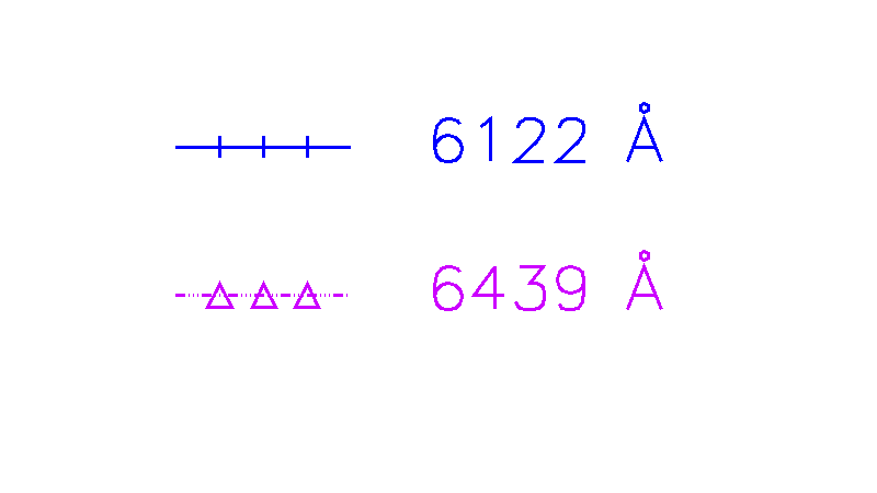
Nights 1 $-$ 4
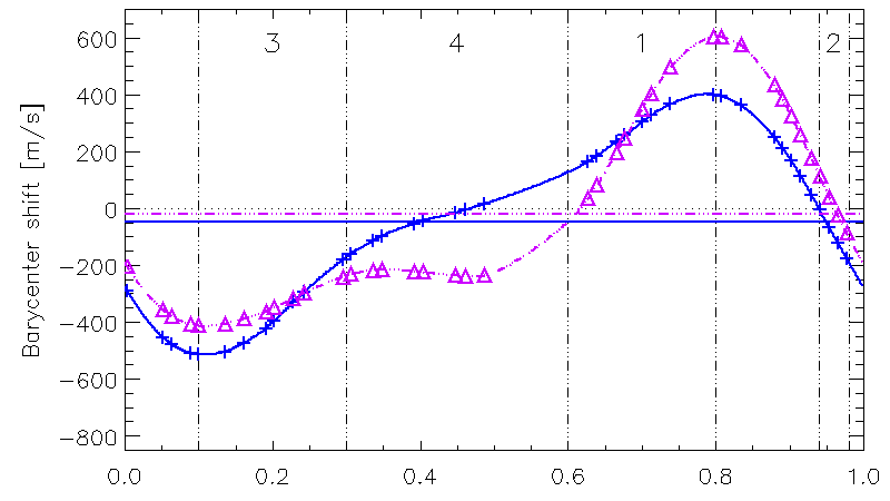
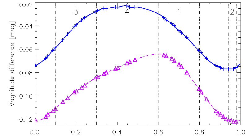
Nights 9 $-$ 12

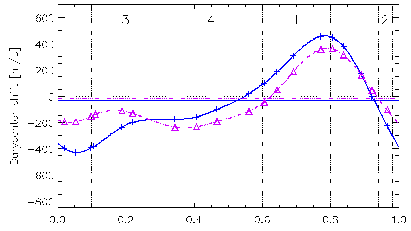
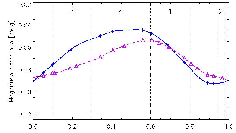
Figure 8: Line barycenters and lightcurves of V889 Her around $\mathrm{JD}_{0}\,+\,4\,000$. On top the observed RV curve is presented (interval (c) of Fig. 6). Left column: Line barycenters computed from our DI line profile reconstructions (see Sect. 6.3); they all show an activity-induced Rossiter-McLaughlin effect matching the observations well. Right column: Lightcurves computed from our Doppler images showing a characteristic correlation to the barycenter modulations. The defined phase intervals $1\,-\,4$ are used in the discussion of Sect. 6.3.2, see also Fig. 9.

Phase 0.8 (Interval 1, end)

Phase 0.95 (Interval 2, center)

Phase 0.1 (Interval 3, start)

Phase 0.45 (Interval 4, center)

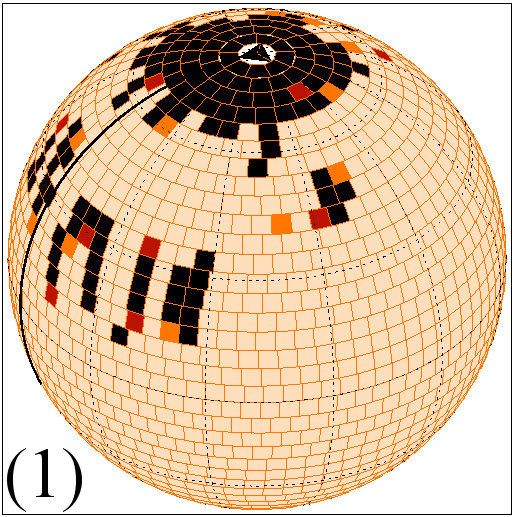
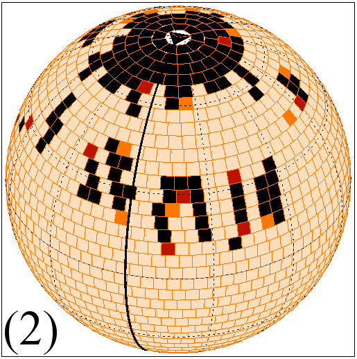
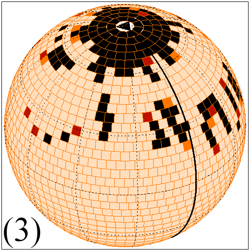
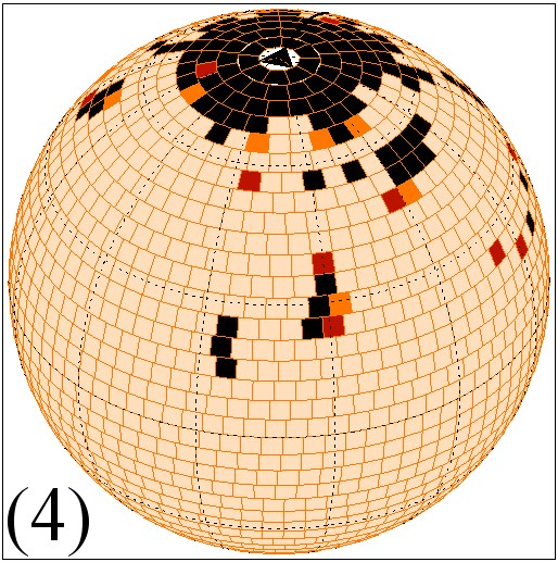
Figure 9: Doppler image of V889 Her (nights $1\,-\,4$, 6439 Å line, see Fig. 7) shown at selected phases that serve the discussion of RV curves of Fig. 8. The phase intervals 1 to 4 annotated on top of each panel are defined there. The sequence illustrates the movement of the dominant spot group (region B) across the visible disk: full visibility at the left limb (1), centered on the stellar disk (2), and movement to the right limb (3). In panel (4) the spot group is located at the back side of the star. Qualitatively, the same sequence can be followed in all our Doppler images.

6.3 RV shifts and lightcurves obtained by Doppler Imaging

For our Doppler images we found ourselves in the unusual situation that we had contemporaneous precise and time-resolved RV measurements. In the following we describe how these can be used to obtain activity information and how they can be compared to Doppler maps.

6.3.1 Approach

Asymmetric deformations of a line profile lead to an apparent radial velocity shift of the line. To quantify such profile asymmetries, we define the center of a line profile as its ‘barycenter’: if $x$ is the radial velocity measured in units of $v\sin(i)$ and $y(x)$ is the corresponding (normalized) flux, we can write down the equation

$$S\ =\ -\sum\limits_{i=1}^{N}\frac{x_{i}\ y(x_{i})\ \Delta x}{W_{\mathrm{Eq}}}\ =\ -\frac{2\ x_{\mathrm{max}}}{N\ W_{\mathrm{Eq}}}\sum\limits_{i=1}^{N}x_{i}\ y(x_{i})\ .$$ (3)

$S$ denotes the barycenter of a line profile in analogy to the barycenter of a system of masses, $W_{\mathrm{Eq}}$ is the spectral line’s equivalent width, and $\Delta x$ is the interval between $x_{i}$ and $x_{i+1}$. Applying Eq. 3 to our reconstructed line profiles computed from our DI, we obtain a measure for the asymmetry-induced shift of the line center as a function of rotation phase. Note that this is not necessarily the same value as derived in standard RV measurements. Nevertheless, as shown in Fig. 8, in our case both approaches yield similar RV curves for the same object. This similarity encompasses amplitude and shape of the RV curves. Eq. 3 is discussed in detail in Appendix A, see also Ohta et al. (2005).

Although we do not have contemporaneous photometry, we compute lightcurves from our images mainly for two reasons. First, as Fig. 8 illustrates, they facilitate the interpretation of the RV curves. Second, they can be compared qualitatively to the Hipparcos lightcurves of Figs. 3 and 4, regarding both amplitude and shape. Using the pre-defined spot continuum flux and limb darkening law, it is straight forward to compute a lightcurve from our Doppler maps. For each rotation phase a disk-integrated flux $f_{i}$ is calculated and transformed to magnitudes using $m\ =\ -2.5\log(f_{i}/f_{0})$ with $f_{0}\ =\ 1$. This results in a magnitude difference $\Delta m\ =\ m-m_{0}$, where $m_{0}$ is the integrated flux over the unspotted surface. This procedure has been shown to yield rather accurate lightcurve fits (Wolter et al., 2008).

6.3.2 Results

We present the lightcurves and line barycenters computed from our Doppler images in Fig. 8. To assist discussion, we introduce phase intervals labeled 1 to 4. Each interval represents a characteristic position of the dominant spot group on the visible stellar disk. The appearance of the visible disk during these phase intervals is illustrated in Fig. 9.

The RV curve of V889 Her, whose observation time interval encompasses that of our Doppler images, is placed at the top of Fig. 8. It was observed during a time span of roughly $500$ days, although most data points come from a limited interval of about $150$ days (interval (c) of Fig. 6). It shows variations of the measured RV that appear largely stable over the selected time interval with a peak-to-peak amplitude of about $1\,000$ m/s.

All RV curves on the left side of Fig. 8 have a similar shape. Their structure is similar to the one expected from an activity-induced Rossiter-McLaughlin effect (see Sects. 5.1 and 5.3).

Interval 1, starting at about phase 0.6, marks the main increase in $S$. During this interval the spot region B (containing the dominant feature) appears at the limb of the visible stellar disk. This leads to a decreased absorption in the blue line wing, causing an apparent RV shift towards longer wavelengths. This shift increases while the entire spotted region rotates onto the disk, which is illustrated in panel (1) of Fig. 9, then decreases again and finally drops to zero in interval 2, when the spot region B is centered on the stellar disk (panel (2)).

After interval 2, the spot region B moves towards the other edge of the stellar disk and influences the star’s redshifted light. The normalized absorption at higher wavelengths is reduced leading to an apparent RV shift towards lower wavelengths. This shift reaches its maximum when region B is located at the ‘red’ edge of the stellar disk. When spot region B finally moves off the visible disk, the line barycenter returns back to zero.

The previous discussion only covered the influence of the large spot feature located at B, which dominates the shape of the RV curves. However, other spotted regions influence the RV curve as well as can especially be seen in interval 4; the associated disk appearance is found in panel (4) of Fig. 9. During this phase interval the dominant feature B is on the backside of the star and does not influence our RV curve. Here, spot group D (cf. Fig. 7) dominates the behavior of the line barycenter as its influence is not masked by the much stronger contribution of spot group B.

Summing up, the observed radial velocities (RV curve) and the line barycenters ($S$ curve) show a far-reaching agreement in shape. There is an apparent phase shift of about 0.1 by which the RV curve lags behind the $S$ curves, most pronounced in the position of the maximum. This apparent shift could be due to small-scale variations of the spot pattern during the roughly $100\,-\,200$ rotations covered by this interval of the RV curve. Alternatively, this shift could be caused by small or low-contrast spot groups not reliably reconstructed in our Doppler maps. Apart from this, the RV and $S$ curves even have comparable amplitudes.

In addition to the line barycenters, the right column of Fig. 8 contains the lightcurves computed from our Doppler maps. The rotational evolution discussed above for the RV curves can be completely followed in the lightcurves; zero passages of the former quite precisely coincide with extrema of the latter. A more symmetric lightcurve is associated with a spot distribution in longitude that is also more symmetric. Such a spot distribution, in turn, leads to a more symmetric RV curve. This can, for example, be seen when comparing the $6122$ Å RV and lightcurves of nights $1\,-\,4$ and $9\,-\,12$, respectively.

7 Discussion

Lightcurves, Doppler images and RV measurements represent complementary data sets for the analysis of large-scale surface structures and their temporal evolution. Signatures of activity can be compared and confirmed between them. In accordance with previous authors, our observations show a significant fraction of V889 Her’s surface covered with spots. These are primarily concentrated in large regions near the poles and within two active regions at lower latitudes.

The analysis of the Hipparcos photometry (taken between $1990$ and $1993$) indicates that these active regions were confined to longitudes between 200° to 300° and 80° to 150° for more than two years. Compared to our Doppler images and RV measurements, which show the spot distribution almost 10 years later, we find a qualitatively similar distribution shifted by at least several dozens of degrees in longitude. The center of the dominant feature is located at about 20° longitude. The second active region apparently had much less influence on the RV data; in the Doppler images, where only small signatures of other large spotted regions can be seen, it is located between 150° and 250° longitude. From a global point of view, this is rather similar to the photometric results.

Concerning the inner structure and shape of active regions, which have a maximum diameter of about 30° to 60°, Doppler images yield information our lightcurve models cannot contain. The DI surface maps show asymmetrical and inhomogeneous active regions. These should not be confused with the active regions reconstructed in the lightcurve models where primarily information on longitudinal position, and no structure, is obtained. Additionally the latter contain only information averaged over dozens of rotations. This means that the size of an active region represents the temporally averaged area of the star with high activity; its ‘center’ indicates the position with highest activity on average. The quality of our fit clearly indicates that the temporal changes are only minor compared to the depths of the minima, and we show that our models present statistically credible reconstructions of the photometry, even though the poor phase sampling and the long time basis of the Hipparcos observations complicate the interpretation of this data set.

Previously, surface reconstructions of V889 Her had been derived by Strassmeier et al. (2003) and Marsden et al. (2006). Their main characteristics do not significantly differ from our Doppler images showing large polar spots down to almost 60° latitude and a few smaller spots at about 30° latitude. The sizes are comparable as well and lie between about 20° to 30°; the dominant feature of our reconstructions may even have a size of almost 60° in diameter (at least in longitudinal direction), although a possible multi-component structure cannot be ruled out. A closer look even reveals some similarity to our lightcurve models. The reconstructions of both authors show dominant surface features at about 300° longitude which roughly agrees with the location of one of our active regions. Unfortunately this is very likely only a coincidence since the long time distance between the different observations leads to phase errors of about 0.1 to 0.3 due to the rotation period’s error (see Sect. 5.2). This makes it hard to compare the spots’ positions in different surface maps directly.

While Marsden et al. (2006) observe differential rotation on this star, in our data sets we do not find any evidence in favor of or against it. The quality of our Doppler imaging data and reconstructions does not allow to significantly constrain differential rotation, mostly because of their lack of well-defined and asymmetric high-latitude spots. The interpretation of the lightcurves does not require the introduction of differential rotation, although it does not exclude it as well; statistically a rigid rotation model is sufficient. However, if strong differential rotation measured by Marsden et al. (2006) also applies to the time span of our RV and photometric data sets, this implies that the dominant spots are confined to a rather narrow latitude band close to about $30$° latitude.

To compare the modulation of high-precision RV measurements to spot distributions, we present a method to determine RV shifts from DI line profile reconstructions. In this process the shifted line center of an asymmetric profile is compared to the RV shift derived in standard RV measurement techniques, in our case from iodine cell spectra. Our results show a striking agreement of this method with the conventional RV measurements, not only qualitatively but quantitatively as well. This provides strong empirical evidence that both methods do not only produce comparable but equal results. Their differences primarily derive from reconstruction errors of the DI line profiles. An illustrative example of a complicated spot distribution causing the superposition of activity-induced Rossiter-McLaughlin effects is presented in this paper. This is only possible due to the availability of Doppler images and contemporaneous high-precision RV measurements.

8 Summary

Using the example of the solar-type, fast rotating star V889 Her, we show that high-accuracy RV measurements can be used to study stellar activity, in particular large-scale spot distributions.

The modulation of V889 Her’s RV curve with a period of $P\,=\,1.3372\,\pm\,0.0004$ days confirms Strassmeier et al.’s rotation period of $P\,=\,1.3371\,\pm\,0.0002$ days. Our data are consistent with no differential rotation; if present, the spots must be confined to a limited range of latitudes. A large subinterval of the data yields a stable and characteristic RV curve due to an activity-induced Rossiter-McLaughlin effect.

This curve is compared to contemporaneous Doppler images. RV shifts derived from different surface reconstructions match the RV observations well confirming that the observed RV modulation is caused by large-scale and long-term stable spotted regions. This also shows that RV shifts can reliably be determined from line profiles reconstructed in the DI process.

Furthermore we confirm the long-term stability of large-scale surface structures on V889 Her modeling the Hipparcos photometry. Pronounced lightcurve minima preserve their position almost unchanged throughout most of the Hipparcos observations. They are associated with two large active regions located at approximately constant longitude but slowly changing size and latitude.

From our analysis we derive different time scales for structures of different sizes. The evolution of ‘small scale’ structures inside active regions is not resolved in our data, although the Doppler images indicate that spots of smaller sizes down to approximately 15° occur. In some cases sizes and longitudes of active regions remain basically unchanged for up to 300 days. The global configuration of a polar spot and two large, clearly separated spot groups apparently existed for more than two years; these two spot groups even remained at largely constant longitudes.

Judging from the Doppler images of this paper and those of other authors (Strassmeier et al. 2003, Marsden et al. 2006), the polar spot is likely to be the most persistent surface feature with a lifetime of at least several years. This is also confirmed by the practically constant maximum brightness observed in the Hipparcos photometry.

Appendix A Analytic proof of equation 3

In Sect. 6.3 we introduce Eq. 3 for the barycenter of a spectral line in analogy to the barycenter determination of a system of masses $x_{s}\,=\,(\sum_{i}x_{i}\ m_{i})/M$, where $M\,=\,\sum_{i}m_{i}$. We start with the continuous representation of Eq. 3, which reads

$$S\ =\ \frac{1}{W_{\mathrm{Eq}}}\int\limits_{-x_{\mathrm{max}}}^{+x_{\mathrm{max}}}x\ \Big{[}1-y(x-x_{c})\Big{]}\ dx\ =\ x_{c},$$ (4)

with $x$ denoting the radial velocity axis and $y(x)$ representing the normalized intensity ($0\leq y\leq 1$). $x_{c}$ is the center position of the line, which we show is equal to the barycenter $S$. Note that the equivalent width, $W_{\mathrm{Eq}}\,=\,\int(1-y(x_{i}))\,dx$, appears by full analogy with the total mass, $M$, here, and we presume it to be constant. The line shape described by $y(x)$ can be arbitrary as long as the integral $\int(1-y(x_{i}))\,dx$ exists; however, the radial velocity axis must be chosen so that $\int x\,(1-y(x))\,dx=0$.

Now we aim at proving the correctness of the last equality in Eq. 4. Note that with this definition $(1-y(x))/W_{\mathrm{Eq}}$ becomes a distribution function; from the mathematical point of view the integration boundaries may easily be extended to cover an arbitrarily large range, however, in the analysis of real data we usually favor tight boundaries to avoid contamination. Therefore, we explicitly consider them here and, further, restrict ourselves to small shifts, $x_{c}\,\ll\,x_{\mathrm{max}}$.

Recasting Eq. 4 we obtain

$$S \ =\ -\frac{1}{W_{\mathrm{Eq}}}\int\limits_{-x_{\mathrm{max}}}^{+x_{\mathrm{max}}}x\ y(x-x_{c})\ dx$$

with the substitution $a\,=\,x-x_{c}$

$$S \ =\ -\frac{1}{W_{\mathrm{Eq}}}\int\limits_{-x_{\mathrm{max}}-x_{c}}^{+x_{\mathrm{max}}-x_{c}}(a+x_{c})\ y(a)\ da$$

$$\ =\ -\frac{1}{W_{\mathrm{Eq}}}\int\limits_{-x_{\mathrm{max}}-x_{c}}^{+x_{\mathrm{max}}-x_{c}}\Big{[}a\ y(a)\ +\ x_{c}\ y(a)\Big{]}\ da\ .$$ (5)

Above, $x_{c}$ represents an arbitrarily signed shift of the line’s center, which we in the following define as positive without loss of generality.

We discuss the two terms of Eq. 5 separately. The first can be treated as follows:

$$-\frac{1}{W_{\mathrm{Eq}}}\int\limits_{-x_{\mathrm{max}}-x_{c}}^{+x_{\mathrm{max}}-x_{c}}a\ y(a)\ da\ =$$

$$-\frac{1}{W_{\mathrm{Eq}}}\left(\underbrace{\int\limits_{-x_{\mathrm{max}}-x_{c}}^{-x_{\mathrm{max}}+x_{c}}a\ y(a)\ da}_{\approx\ -2x_{c}x_{\mathrm{max}}}+\underbrace{\int\limits_{-x_{\mathrm{max}}+x_{c}}^{+x_{\mathrm{max}}-x_{c}}a\ y(a)\ da}_{=\ 0}\right)\ .$$

In the approximation of the first integral we applied the relation $y(a)\,\approx\,1$, which is valid within the integration interval ($x_{\mathrm{max}}$ must be chosen accordingly), and the second integral is zero by definition.

We resume with the second term of Eq. 5:

$$-\frac{1}{W_{\mathrm{Eq}}}\int\limits_{-x_{\mathrm{max}}-x_{c}}^{+x_{\mathrm{max}}-x_{c}}x_{c}\ y(a)\ da \ =\ -\frac{x_{c}}{W_{\mathrm{Eq}}}\left(2x_{\mathrm{max}}-W_{\mathrm{Eq}}\right)$$

$$\ =\ -\frac{2\,x_{\mathrm{max}}\,x_{c}}{W_{\mathrm{Eq}}}+x_{c}\ .$$

For the last calculations we use

$$W_{\mathrm{Eq}}\ \approx\int\limits_{-x_{\mathrm{max}}-x_{c}}^{+x_{\mathrm{max}}-x_{c}}\Big{(}1-y(a)\Big{)}\ da\ =\ 2x_{\mathrm{max}}\,-\int\limits_{-x_{\mathrm{max}}-x_{c}}^{+x_{\mathrm{max}}-x_{c}}y(a)\ da\ .$$

Inserting the result into Eq. 5, the equation

$$S\ =\ \frac{2\,x_{c}\,x_{\mathrm{max}}}{W_{\mathrm{Eq}}}-\frac{2\,x_{c}\,x_{\mathrm{max}}}{W_{\mathrm{Eq}}}+x_{c}\ =\ x_{c}\ \ \mathrm{q.e.d.}$$ (6)

emerges, which is exactly the equality we strove to prove.

Appendix B Cross-correlation of Doppler images

Figure 10 (upper panel) shows the cross-correlation map comparing the Doppler images of Fig. 7, i.e. the reconstructions for nights $1\,-\,4$ and $9\,-\,12$ using line $6122$ and rigid rotation. For each co-latitude the map shows the cross-correlation, normalized to the overall maximum, obtained when shifting the spots of map $9\,-\,12$ by the given longitude angle. Darker orange shades indicate larger correlation values. Crosses mark the correlation maximum for each co-latitude, their values are shown in the right-hand graph, also illustrating the assignment of orange hues. For comparison, the smooth, sine-like curve renders the surface shear resulting from Marsden et al.’s differential rotation law.

Figure 10 (lower panel) shows the same for Doppler images reconstructed adopting Marsden et al.’s differential rotation law. The correlation maps do not support or disprove any specific rotation law.

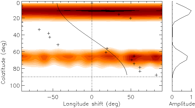
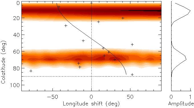
Figure 10: Cross-correlation maps comparing the Doppler images of Fig. 7 (upper panel) and reconstructions using Marsden et al.’s differential rotation law (lower panel). See text for detailed information.

Line 6439 Å, Nights $1\,-\,4$

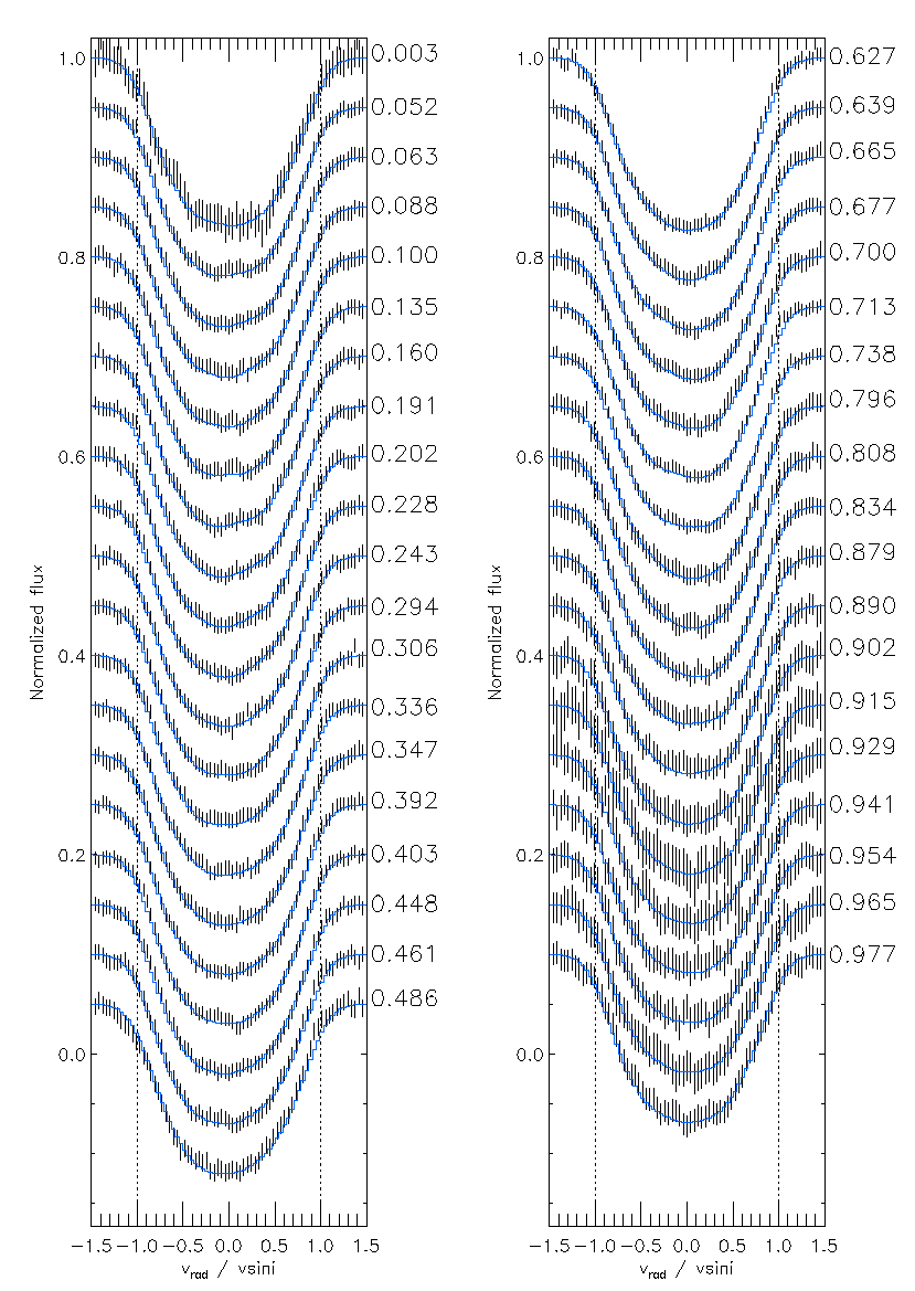
    Line 6439 Å, Nights $9\,-\,12$
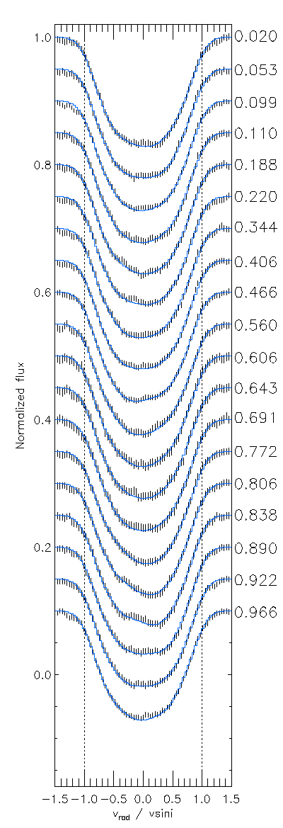
Line 6122 Å, Nights $1\,-\,4$     Line 6122 Å, Nights $9\,-\,12$

Figure 11: Stack plot of all DI line profile reconstructions. The left column shows the $39$ phases of nights $1\,-\,4$, the right column the $19$ phases of the nights $9\,-\,12$ observations. The two upper panels show line 6439 Å, the two lower panels show 6122 Å. See App. C for more details.

Appendix C DI line profile reconstructions

We give the DI line profile reconstructions of all Doppler images presented in Sect. 7. Figure 11 contains the profiles of the 6439 Å (top panels) and the 6122 Å(bottom panels) Ca I lines, 39 phases for nights $1\,-\,4$ (left column) and 19 phases for nights $9\,-\,12$ (right column). All lines are continuum normalized but shifted in flux by $0.05$ (stacked plot). Rotation phases increase from top to bottom; they are given at the right border. The observed line profiles are shown as vertical lines indicating their observation errors, the DI reconstructions (blue) are overplotted with a straight line. Both are plotted over rotation velocity $v_{\mathrm{rad}}$ in units of $v\sin(i)$.