Relaxed Equilibrium Configurations to Model Fossil Fields
I – A first family

Abstract

Context. The understanding of fossil fields origin, topology and stability is one of the corner stones of the stellar magnetism theory. On one hand, since they survive over secular time-scales, they may modify the structure and the evolution of their host stars. On the other hand, they must have a complex stable structure since it has been demonstrated by Tayler and collaborators that simplest purely poloidal or toroidal fields are unstable on dynamical time-scales. In this context, the only stable configuration which has been found today is the one resulting of a numerical simulation by Braithwaite and collaborators who have studied the evolution of an initial stochastic magnetic field, which is found to relax on a mixed stable configuration (poloidal and toroidal) that seems to be in equilibrium and then diffuses.

Aims. In this work, we thus go on the track of such type of equilibrium field in a semi-analytical way.

Methods. In this first article, we study the barotropic magnetohydrostatic equilibrium states; the problem reduces to a Grad-Shafranov-like equation with arbitrary functions. Those latters are constrained by deriving the lowest-energy equilibrium states for given invariants of the considered axisymmetric problem and in particular for a given helicity which is known to be one of the main actor of such problems. Then, we obtain the generalization of the force-free Taylor’s relaxation states obtained in laboratory experiments (in spheromaks) that become non force-free in the self-gravitating stellar case. The case of general baroclinic equilibrium states will be studied in Paper II.

Results. Those theoretical results are applied to realistic stellar cases, namely to the solar radiative core and to the envelope of an Ap star, and discussed. In both cases we assume that the field is initially confined in the stellar radiation zone.

1 Introduction

Spectropolarimetry is nowadays exploring the stellar magnetism across the whole Hertzsprung-Russel diagram (Donati et al. 1997, 2006; Neiner 2007; Landstreet et al. 2008; Petit et al. 2008). Furthermore, helioseismology and asteroseismology are providing new constraints on internal transport processes occuring in stellar interiors (Turck-Chièze & Talon 2008; Aerts et al. 2008). In this context, even if standard stellar models explain the main features of stellar evolution, it is now crucial to go beyond this modelling to introduce dynamical processes such as magnetic field and rotation to investigate their effects on stellar structure and secular evolution (Maeder & Meynet 2000; Talon 2008). To achieve this aim, secular MHD transport equations have been derived in order to be introduced in stellar evolution codes. They take into account in a coherent way the interaction between differential rotation, turbulence, meridional circulation, and magnetic field (Spruit 2002; Maeder & Meynet 2004; Mathis & Zahn 2005), while non-linear numerical simulations provide new insight on these mechanisms (Charbonneau & MacGregor 1993; Rudiger & Kitchatinov 1997; Garaud 2002; Brun & Zahn 2006). If we want to go further, the simplest modifications of static structural properties such as density, gravity, pressure, temperature, and luminosity induced by the magnetic field have also to be systematically quantified as a function of the field geometry and strength (Moss 1973; Mestel & Moss 1977; Lydon & Sofia 1995; Couvidat et al. 2003; Li et al. 2006; Duez et al. 2008; Li et al. 2009; Duez et al. 2010).

However, an infinity of possible magnetic configurations can be investigated since the different observation techniques only lead to indirect indications on the internal field topologies through the surface field properties they provide. Furthermore, since the simplest geometrical configurations like purely poloidal and purely toroidal fields are known to be unstable (Acheson 1978; Tayler 1973; Markey & Tayler 1973, 1974; Goossens & Veugelen 1978; Goossens & Tayler 1980; Goossens et al. 1981; van Assche et al. 1982; Spruit 1999; Braithwaite 2006, 2007), the best candidates for stable geometries are mixed poloidal-toroidal fields (Wright 1973; Markey & Tayler 1974; Tayler 1980; Braithwaite 2009).

Therefore, it is necessary to go on the track of possible stable magnetic configurations in stellar interiors to evaluate their effects on stellar structure and to use them as potential initial conditions to study secular internal transport processes.

In this work, we thus revisit the pioneer works by Ferraro (1954); Mestel (1956); Prendergast (1956) and Woltjer (1960). Ferraro (1954) studied the equilibrium configurations of an incompressible star with a purely poloidal field. Prendergast (1956) (see also Chandrasekhar 1956a; Chandrasekhar & Prendergast 1956; Chandrasekhar 1956b) then extended the model to take into account the toroidal field, by solving the magneto-hydrostatic equilibrium of incompressible spheres. The obtained configurations seem to be relevant in regard of the most recent numerical simulations that may explain fossil fields in early-type stars, white dwarfs or neutron stars (Braithwaite & Spruit 2004; Braithwaite & Nordlund 2006; Braithwaite 2006) and of theoretical studies of their helicity relaxation (Broderick & Narayan 2008; Mastrano & Melatos 2008). The main generalization of Prendergast’s work we achieve here consists in relaxing the incompressible hypothesis in order to take into account the star’s structure (see also Woltjer 1960), which differs as a function of its stellar type and of its evolution stage, and to derive the minimum energy equilibrium configuration for a given mass and helicity, which are then applied to realistic models of stellar interiors.

Assuming that the Lorentz volumetric force is a perturbation compared with the gravity, we derive the non force-free magnetohydrostatic equilibrium. In this first article, we then focus on the barotropic equilibrium states family , for which the possible field configurations and the stellar structure are explicitely coupled; these may correspond to the numerical experiments by Braithwaite and collaborators. In this case, the problem reduces to a Grad-Shafranov-like equation (Grad & Rubin 1958; Shafranov 1966; Kutvitskii & Solov’ev 1994), similar to the one intensively used in fusion plasma physics. We then focus on its minimum energy eigenmodes for a given mass and helicity, which are derived and applied in order to model relaxed stellar fossil magnetic fields which are found to be non force-free. Arguments in favor of the stability of the obtained configurations are finally discussed (Wright 1973; Tayler 1980; Braithwaite 2009; Reisenegger 2009) and we compare their properties with those of relaxed fields obtained in numerical simulations (Braithwaite 2008). The case of general baroclinic equilibrium states will be studied in Paper II (Wright 1969; Moss 1975).

2 The Non Force-Free Magneto-Hydrostatic Equilibrium

In this work, we focus on the magnetic equilibrium of a self-gravitating spherical shell to model fossil fields in stellar interiors. To achieve this goal, we start from

$$\textbf{{0}}=-\bm{\nabla}P-\rho\bm{\nabla}V+\bm{F}_{\!\mathbf{{\mathcal{L}}}},\,\hbox{where}\,\,\bm{F}_{\!\mathbf{{\mathcal{L}}}}=\textbf{{j}}\times\textbf{{B}}.$$ (1)

Eq. (1) must be satisfied in the interior of an infinitely conducting mass of fluid in the presence of a large-scale field together with the Poisson equation, $\nabla^{2}V=4\>\pi\>G\>\rho$, and the Maxwell equations, $\bm{\nabla}\cdot\textbf{{B}}=0$ (Maxwell flux) and $\bm{\nabla}\>\mathbf{\times}\>\textbf{{B}}=\mu_{0}\>\>\textbf{{j}}$ (Maxwell-Ampère).
$P$, $\rho$ and $V$ are respectively the pressure, the density and the gravitational potential of the considered plasma. B is the magnetic field and j is the associated current, which is given in the classical MHD approximation by the Maxwell-Ampère’s equation. $\mu_{0}$ is the magnetic permeability of the plasma and $\bm{F}_{\!\mathbf{{\mathcal{L}}}}$ is the Lorentz force.

2.1 Magnetic field configuration and the magnetohydrostatic equilibrium

If we consider only the axisymmetric case, where all physical variables are independent of the azimuthal angle ($\varphi$), $\textbf{{B}}\left(r,\theta\right)$ can be written in the form

$$\textbf{{B}}=\frac{1}{r\sin\theta}\bm{\nabla}\Psi\left(r,\theta\right)\mathbf{\times}\,\mathbf{\hat{e}_{\varphi}}+\frac{1}{r\sin\theta}\,F\left(r,\theta\right)\,\mathbf{\hat{e}_{\varphi}}\,,$$ (2)

which is divergenceless. $\Psi$ and $F$ are respectively the poloidal flux function and the toroidal potential; $\left(r,\theta,\varphi\right)$ are the usual spherical coordinates and $\left\{{\bf{\hat{e}}}_{k}\right\}_{k=r,\theta,\varphi}$ their unit-vector basis. Finally, the poloidal component of the magnetic field ($\textbf{{B}}_{\rm P}$) is such that $\textbf{{B}}_{\rm P}\cdot\bm{\nabla}\Psi=0$, so it belongs to iso-$\Psi$ surfaces. The magnetohydrostatic equilibrium (Eq. 1) implies that the poloidal part (in the meridional plane in the axisymmetric case) of the Lorentz force ($\textit{{F}}_{\!\mathbf{{\mathcal{L}}_{P}}}$) balances the pressure gradient and the gravitational force, which are also purely poloidal vectors, while, in the absence of any other force, its toroidal component ($\textit{{F}}_{\!\mathbf{{\mathcal{L}}_{T}}}=\textit{F}_{\!\mathbf{{\mathcal{L}}_{\varphi}}}\bf{\hat{e}}_{\varphi}$) vanishes. We thus have

$$\bm{F}_{\!\mathbf{{\mathcal{L}}}}=\textit{{F}}_{\!\mathbf{{\mathcal{L}}_{P}}}+\textit{F}_{\!\mathbf{{\mathcal{L}}_{\varphi}}}\bf{\hat{e}}_{\varphi}=\textit{{F}}_{\!\mathbf{{\mathcal{L}}_{P}}}.$$ (3)

Using Eq. (2), we obtain

$$\textit{{F}}_{\!\mathbf{{\mathcal{L}}_{P}}}=-\frac{1}{\mu_{0}r^{2}\sin^{2}\theta}\Bigg{\{}\left(F\partial_{r}F+\partial_{r}\Psi\Delta^{*}\Psi\right){\bf\hat{e}}_{r}$$

$${+\frac{1}{r}\left(F\partial_{\theta}F+\partial_{\theta}\Psi\Delta^{*}\Psi\right){\bf\hat{e}}_{\theta}\Bigg{\}}},$$ (4)

with $\partial_{x}=\partial/\partial x$, and

$$\Delta^{*}\Psi\equiv\partial_{rr}{\Psi}+\frac{\sin\theta}{r^{2}}\partial_{\theta}\left(\frac{1}{\sin\theta}\partial_{\theta}{\Psi}\right)$$ (5)

is the usual Grad-Shafranov operator in spherical coordinates. On the other hand, since $\textit{F}_{\!\mathbf{{\mathcal{L}}_{\varphi}}}=0$, we get $\partial_{r}\Psi\partial_{\theta}F-\partial_{\theta}\Psi\partial_{r}F=0$; the non-trivial values for $F$ are therefore obtained by setting

$$F(r,\theta)=F(\Psi).$$ (6)

Then, we obtain $F\partial_{r}{F}=F\partial_{\Psi}F\partial_{r}\Psi$ and $F\partial_{\theta}{F}=F\partial_{\Psi}F\partial_{\theta}\Psi$, leading to the final expansion of the Lorentz force

$$\textit{{F}}_{\!\mathbf{{\mathcal{L}}}}={\mathcal{A}}\left(r,\theta\right)\bm{\nabla}\Psi,$$ (7)

where

$${\mathcal{A}}(r,\theta)=-\frac{1}{\mu_{0}r^{2}\sin^{2}\theta}\left(F\partial_{\Psi}F+\Delta^{*}\Psi\right).$$ (8)

Therefore, the poloidal component of $\textit{{F}}_{\!\mathbf{{\mathcal{L}}}}$ is nonzero a priori, the field being thus non force-free in this case.

This point has here to be discussed. First, Reisenegger (2009) demonstrated that the magnetic field can not be force-free everywhere in stellar interiors (see the demonstration in the appendix A of his paper). Note in this context that the “force-free” configurations obtained by Broderick & Narayan (2008) verify this theorem because they have current sheets with a non-zero Lorentz force on the stellar surface. Moreover, Shulyak et al. (2007, 2009) showed how the atmosphere of a CP star can be the host of a non-zero Lorentz force. Therefore, from now on, we consider the non force-free equilibrium.

Now, if we take the curl of Eq. (1), we get the static vorticity equation

$$-\frac{\bm{\nabla}\,\rho\times\bm{\nabla}\,P}{\rho^{2}}=\bm{\nabla}\times\left(\frac{\textit{{F}}_{\!\mathbf{{\mathcal{L}}}}}{\rho}\right),$$ (9)

that governs the balance between the baroclinic torque (left-hand side; see Rieutord (2006) for a detailed description) and the magnetic source term. Then, as has been emphasized by Mestel (1956), the different structural quantities such as the density, the gravitational potential, and the pressure relax in order to verify Eq. (1) for a given field configuration (see Sweet (1950); Moss (1975), and Mathis & Zahn (2005) §5.). Thus, the choice for $\Psi$ is left free.

2.2 The barotropic equilibrium state family

Magnetic initial configurations are one of the crucial unanswered question for the modelling of MHD transport processes in stellar interiors. To examine this question, Braithwaite and collaborators (Braithwaite & Spruit 2004; Braithwaite & Nordlund 2006) studied the relaxation of an initially stochastic field in models of convectively stable stellar radiation zones. The field is found to relax, after several Alfvén times, to a mixed poloidal-toroidal equilibrium configuration, which then diffuses towards the exterior.

We choose here, using an analytical approach, to find such field geometries, which are governed at the beginning by the magnetohydrostatic equilibrium.

To achieve this aim, we focus in this first article on the particular barotropic equilibrium states (in the hydrodynamic meaning of the term) for which the field configuration is explicitely coupled with the stellar structure, since we have in this case

$$-\frac{\bm{\nabla}\,\rho\times\bm{\nabla}\,P}{\rho^{2}}=\bm{\nabla}\times\left(\frac{\textit{{F}}_{\!\mathbf{{\mathcal{L}}}}}{\rho}\right)=\textbf{{0}}.$$ (10)

Those are the generalization of the Prendergast’s equilibria which take into account the compressibility and which have been studied in polytropic cases by Woltjer (1960); Wentzel (1961); Roxburgh (1966); Monaghan (1976).

Let us first recall the definition of the barotropic states. In fluid mechanics, a fluid is said to be in a barotropic state if the following condition is satisfied (see Pedlosky (1998) in a geophysical context and Zahn (1992) in a stellar one):

$$\bm{\nabla}\rho\times\bm{\nabla}P={\textbf{{0}}};$$ (11)

in other words, the baroclinic torque in the vorticity equation (Eq. 9) vanishes. Then, the surfaces of equal density coincide with the isobars since the density and the pressure gradients are aligned. This does not imply any question of equation of state, which in stellar interiors can take the most general form $P=f\left(\rho,T,\cdot\!\cdot\!\cdot\,\right)$ ($T$ being the temperature). Moreover, this does not presume anything about the stratification of the fluid, which can be stably stratified or not. For example, a star in solid body rotation is in a barotropic state (as opposed to baroclinic) (see once again Zahn 1992). Let us illustrate this point with the simplest case of a non-rotating and non-magnetic stellar radiation zone. In this case, the hydrostatic balance is given by ${\bm{\nabla}P}/{\rho}=-\bm{\nabla}V={\textbf{{g}}}$. If we take the curl of this equation, we obtain the stationary version of the thermal-wind equation:

$$-\frac{\bm{\nabla}\rho\times\bm{\nabla}P}{\rho^{2}}=-\bm{\nabla}\times\left[\bm{\nabla}V\right]={\textbf{{0}}}$$ (12)

and the star is thus in a barotropic state in the hydrodynamic meaning of the term.

This has to be distinguished from the point of view of thermodynamics where a barotropic equation of state is such that $P=f\left(\rho\right)$ while a non-barotropic equation of state is such that $P=f\left(\rho,T,\cdot\!\cdot\!\cdot\,\right)$.

Then, it is clear that a fluid with a barotropic equation of state is automatically in an hydrodynamical barotropic state. However, in the case of a fluid with a non-barotropic equation of state, the situation is more subtle: in the case where the curl of the volumetric perturbing force vanishes (i.e. $\bm{\nabla}\times\left({\textit{{F}}_{\!\mathbf{{\mathcal{L}}}}}/{\rho}\right)=0$) the fluid is in an hydrodynamical barotropic state, while in the general case it is in a baroclinic situation. Then, a fluid with a non-barotropic equation of state can be in a barotropic state even if it is only for a specific form of the perturbing force. In this first work, we choose to examine the first equilibrium family in which the Lorentz force verify the barotropic balance described by Eq. (11) in a stably stratified radiation zone. The second general case (cf. Mestel 1956) will be studied in paper II.

Stellar interiors, except just under the surface, are in a regime where $\beta=P/P_{\rm Mag}\!>\!\!>\!1$, $P_{\rm Mag}=B^{2}/(2\,\mu_{0})$ being the plasma’s magnetic pressure. On the other hand, in the domain of fields amplitudes relevant for classical stars (i.e. the non-compact objects), the ratio of the volumetric Lorentz force by the gravity is very weak. Therefore, the stellar structure modifications induced by the field can be considered as perturbations only from a spherically symmetric background (Haskell et al. 2008). Then, we can write $\rho\approx\overline{\rho}+\widetilde{\rho}$, where $\overline{\rho}$ and $\widetilde{\rho}$ are respectively the mean density on an isobar, which is given at the first order by the standard non-magnetic radial density profile of the considered star, and its magnetic-induced perturbation on the isobar (with $\widetilde{\rho}\!<\!\!<\!\overline{\rho}$). Thus to the first order, Eq. (10) on an isobar becomes

$$-\frac{\bm{\nabla}\widetilde{\rho}\times\textbf{{g}}_{\rm eff}}{\overline{\rho}}=\bm{\nabla}\times\left(\frac{\textit{{F}}_{\!\mathbf{{\mathcal{L}}}}}{{\overline{\rho}}}\right)=\textbf{{0}},$$ (13)

where the effective gravity $({\textbf{{g}}}_{\rm eff})$, such that $\bm{\nabla}\overline{P}=\overline{\rho}\>{\textbf{{g}}}_{\rm eff}$, has been introduced. This gives, using Eq. (7)

$$\bm{\nabla}\left(\frac{\mathcal{A}}{\overline{\rho}}\right)\times\bm{\nabla}\Psi={\textbf{{0}}},$$ (14)

which projects only along $\mathbf{\hat{e}_{\varphi}}$ as

$$\partial_{r}\left(\frac{\mathcal{A}}{\overline{\rho}}\right)\partial_{\theta}\Psi-\partial_{\theta}\left(\frac{\mathcal{A}}{\overline{\rho}}\right)\partial_{r}\Psi=0,$$ (15)

so that there exists a function $G$ of $\Psi$ such that

$$\frac{\mathcal{A}}{\overline{\rho}}=G\left(\Psi\right).$$ (16)

Then, Eq. (8) leads to the following one ruling $\Psi$

$$\Delta^{*}\Psi+F\left(\Psi\right)\partial_{\Psi}\left[F\left(\Psi\right)\right]=-\mu_{0}r^{2}\sin^{2}\theta\,\overline{\rho}\,G\left(\Psi\right).$$ (17)

This equation is similar to the well-known Grad-Shafranov equation which is used to find equilibria in magnetically confined plasmas such as those in tokamaks or in spheromaks (Grad & Rubin 1958; Shafranov 1966). However, here the source term is different and is directly related to the internal structure of the star through its density profile ($\overline{\rho}$) (the general form of the Grad-Shafranov equation in an astrophysical context is discussed for example in Heinemann & Olbert (1978) and Ogilvie (1997)). Moreover, since the field has to be non force-free in stellar interiors $G\neq 0$ (see the previous discussion in §2.1. and Eqs. 16, 7 and 8).

It is only applicable to the case of the barotropic state family. The equations for the general case will be studied in paper II.

2.3 F and G expansion

Let us now focus on the respective expansion of $F$ and $G$ as a function of $\Psi$.

First, since $F$ is a regular function, we can expand it in power series in $\Psi$:

$$F(\Psi)=\sum_{i=0}^{\infty}\frac{\lambda_{i}}{R}\Psi^{i},$$ (18)

the $\lambda_{i}$ being the expansion coefficients that have to be determined and $R$ a characteristic radius which will be identified below. On the other hand, $B_{\varphi}$ must be regular at the center of the sphere; the first term ($i=0$) of the previous expansion is then excluded (cf. Eq. 2), the above expansion thus reducing to $F(\Psi)=\sum_{i>0}\left(\lambda_{i}/R\right)\Psi^{i}$.

In the same way, $G$ can be expanded as

$$G\left(\Psi\right)=\sum_{j=0}^{\infty}\beta_{j}\Psi^{j}.$$ (19)

Then, Eq. (17) becomes:

$$\Delta^{*}\Psi+\sum_{k>0}\frac{\Lambda_{k}}{R^{2}}\Psi^{k}=-\mu_{0}r^{2}\sin^{2}\theta\,\overline{\rho}\,\sum_{j=0}^{\infty}\beta_{j}\Psi^{j},$$ (20)

where $\Lambda_{k}=\sum_{i_{1}>0}\sum_{i_{2}>0}\left\{i_{2}\lambda_{i_{1}}\lambda_{i_{2}}\delta_{i_{1}+i_{2}-1,k}\right\}$, $\delta$ being the usual Kronecker symbol. This is the generalization of the Grad-Shafranov-type equation obtained by Prendergast (1956) for the barotropic compressible states.

Thus, having assumed the non force-free barotropic magneto-hydrostatic equilibrium state leads to undetermined arbitrary functions ($F$ and $G$) that must be constrained. To achieve this aim, we follow the method given in the axisymmetric case by Chandrasekhar & Prendergast (1958) and Woltjer (1959b) that allows to find the equilibrium state of lowest energy compatible with the constancy of given invariants for the studied axisymmetric system.

3 Self-Gravitating Relaxation States

3.1 Definitions and axisymmetric invariants

We first introduce the cylindrical coordinates $\left(s,\varphi,z\right)$ where $s=r\sin\theta$ and $z=r\cos\theta$. Then, B given in Eq. (2) becomes

$$\textbf{{B}}\left(s,z\right)=\frac{1}{s}\bm{\nabla}\Psi\left(s,z\right)\times\,\mathbf{\hat{e}_{\varphi}}+\frac{1}{s}F\left(s,z\right)\,\mathbf{\hat{e}_{\varphi}}.$$ (21)

Then, we define the potential vector $\textbf{{A}}\left(s,z\right)=A_{\varphi}\left(s,z\right)\mathbf{\hat{e}_{\varphi}}$ such that $\textbf{{B}}_{\rm P}=\bm{\nabla}\times\textbf{{A}}$ and we get

$$\textbf{{B}}=\bm{\nabla}\times{\textbf{{A}}}+\frac{F}{s}\mathbf{\hat{e}_{\varphi}}\quad\hbox{where}\quad A_{\varphi}\left(s,z\right)=\frac{\Psi}{s}.$$ (22)

Next, we insert the expansion for the magnetic field B used by Chandrasekhar & Prendergast (1958) and Woltjer (1959a, b):

$$\textbf{{B}}=-s\>\partial_{z}{\Phi}\left(s,z\right)\mathbf{\hat{e}_{s}}+\!\frac{1}{s}\partial_{s}\left[s^{2}{\Phi}\left(s,z\right)\right]\mathbf{\hat{e}_{z}}+s\>{\mathcal{T}}\left(s,z\right)\mathbf{\hat{e}_{\varphi}}$$ (23)

where $\left\{\widehat{\textbf{{e}}}_{k}\right\}_{k=s,\varphi,z}$ is the cylindrical unit-vector basis and where we identify using Eq. (21)

$$\Psi=s^{2}{\Phi}\quad\hbox{and}\quad F=s^{2}{\mathcal{T}}.$$ (24)

The Grad-Shafranov operator applied to $\Psi$ can then be expressed as follow

$$\Delta^{*}\Psi=s^{2}\>\bm{\nabla}\cdot\left(\frac{\bm{\nabla}\Psi}{s^{2}}\right)=\left[\partial_{ss}\!-\!\frac{1}{s}\partial_{s}\!+\!\partial_{zz}\right]\Psi=s^{2}\Delta_{5}\Phi,$$ (25)

where $\Delta_{5}=\partial_{ss}+\frac{3}{s}\partial_{s}+\partial_{zz}.$

We now introduce the two general families of invariants of the barotropic axisymmetric magneto-hydrostatic equilibrium states, which have been introduced by Woltjer (1959b) for the compressible case (see also Wentzel 1960):

$${\mathcal{I}}_{{\rm I};n}=\int_{\mathcal{V}}M_{n}\left(s^{2}\Phi\right){\overline{\rho}}\,{\rm d}{\mathcal{V}}=\int_{\mathcal{V}}\left(s^{2}\Phi\right)^{n}{\overline{\rho}}\,{\rm d}{\mathcal{V}},$$ (26)

$${\mathcal{I}}_{{\rm I\!I};q}=\int_{\mathcal{V}}N_{q}\left(s^{2}\Phi\right)\,{\mathcal{T}}\,{\rm d}{\mathcal{V}}=\int_{\mathcal{V}}\left(s^{2}\Phi\right)^{q}{\mathcal{T}}\,{\rm d}{\mathcal{V}},$$ (27)

where $M_{n}$ and $N_{q}$ are arbitrary functions that have to be specified. Those latters are conserved as long as

$$\textbf{{B}}\cdot\widehat{\textbf{{e}}}_{r}=0\quad\hbox{(\it i.e. }\Phi={\mathcal{T}}=0)$$ (28)

on the boundaries.

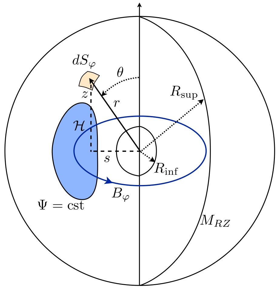
Figure 1: Schematic representation of the two coordinates systems used and of a constant $\Psi$ surface. The invariants of the axisymmetric system are the total mass of the considered stellar radiative region ($M_{\rm RZ}$), the mass enclosed in a constant $\Psi$ surface, the toroidal flux ($\mathcal{F}_{\varphi}$) associated with the toroidal magnetic field ($B_{\varphi}$), and the global helicity ($\mathcal{H}$).

3.2 Fossil fields barotropic relaxation states

Let us first concentrate on ${\mathcal{I}}_{{\rm I\!I};q}$ and $N_{q}$ relevant for fossil fields relaxation. First, if we set $N_{0}\left(s^{2}\Phi\right)=1$, we obtain

$${\mathcal{I}}_{{\rm I\!I};0} = \int_{\mathcal{V}}{\mathcal{T}}\,{\rm d}{\mathcal{V}}=2\,\pi\int_{\mathcal{S}}B_{\varphi}{\rm d}s{\rm d}z$$ (29)

$$= 2\,\pi\int_{\mathcal{S}}B_{\varphi}\>{\rm d}{\mathcal{S}}_{\varphi}=2\,\pi\>{\mathcal{F}}_{\varphi}$$

that corresponds to the conservation of the flux of the azimuthal field across the meridional plane of the star (${\mathcal{F}}_{\varphi}$) in perfect axisymmetric MHD equilibria.

Then, if we set $N_{1}\left(s^{2}\,\Phi\right)=s^{2}\,\Phi$, we get

$${\mathcal{I}}_{\rm I\!I;1}=\int_{\mathcal{V}}\left(s^{2}\,\Phi\right){\mathcal{T}}\,{\rm d}{\mathcal{V}}=\int_{\mathcal{V}}A_{\varphi}B_{\varphi}{\rm d}{\mathcal{V}}={\mathcal{H}}/2,$$ (30)

where we thus identify the magnetic helicity (${\mathcal{H}}$; see §5.1.) of the field configuration which is a global quantity integrated over the volume of the studied radiation zone.

Let us briefly discuss the peculiar role of this quantity in the search of stable equilibria. As emphasized by Spruit (2008), the magnetic helicity is a conserved quantity in a perfectly conducting fluid with fixed boundary conditions. However, in realistic conditions, rapid reconnection can take place even at very high conductivity, especially when the field is dynamically evolving, for example during its initial relaxation phase. Nevertheless, in laboratory experiments, like for example in spheromaks, the helicity is often observed to be approximately conserved, which leads to the existence of stable equilibrium configurations. In fact, if the helicity is conserved a dynamical or unstable field with a finite initial helicity (${\mathcal{H}}_{0}$) cannot decay completely, the helicity of vanishing field being zero. This is precisely what has been observed in the numerical experiment performed by Braithwaite & Spruit (2004) and Braithwaite & Nordlund (2006), where an initial stochastic field with a finite helicity decays initially but relaxes into a stable equilibrium.

In the context of laboratory low-$\beta$ plasmas, this process has been identified by Taylor (1974) and is thus called the Taylor’s relaxation.

For this reason, we now search as Chandrasekhar & Prendergast (1958) the final state of equilibrium, which is the state of lowest energy that the compressible star, preserving its axisymmetry, can attain while conserving the invariants ${\mathcal{I}}_{{\rm I};n}$, ${\mathcal{I}}_{\rm I\!I;0}={\mathcal{F}}_{\varphi}$ and ${\mathcal{I}}_{\rm I\!I;1}={\mathcal{H}}/2$ in barotropic states.

To achieve this, we thus introduce the total energy of the system

$$E = \frac{1}{2}\int_{\mathcal{V}}\left\{\frac{{\textbf{{B}}}^{2}}{\mu_{0}}+{\rho}\left[V+2{\mathcal{U}}\right]\right\}{\rm d}{\mathcal{V}}$$

$$= \frac{1}{2}\int_{\mathcal{V}}\left\{\frac{1}{\mu_{0}}\left[-s^{2}\Phi\Delta_{5}\Phi+s^{2}{\mathcal{T}}^{2}\right]+{\rho}\left[V+2{\mathcal{U}}\right]\right\}{\rm d}{\mathcal{V}},$$

where ${\mathcal{U}}$ is the specific internal energy per unit mass (Woltjer 1958, 1959b; Broderick & Narayan 2008). To obtain the minimal energy equilibrium state for the given invariants ${\mathcal{I}}_{{\rm I};n}$ and a given helicity and azimuthal flux, we thus minimize $E$ with respect to ${\mathcal{I}}_{{\rm I};n}$, ${\mathcal{I}}_{\rm I\!I;0}$ and ${\mathcal{I}}_{\rm I\!I;1}$. This leads, introducing the associated Lagrangian multipliers $\left(a_{{\rm I};n},a_{{\rm I\!I};0},a_{{\rm I\!I};1}\right)$, to the following condition for a stationary energy:

$$\delta E+\sum_{n}a_{{\rm I};n}\>\delta{\mathcal{I}}_{{\rm I};n}+\sum_{q=0}^{1}a_{{\rm I\!I};q}\>\delta{\mathcal{I}}_{{\rm I\!I};q}=0.$$ (32)

Following the method described in Chandrasekhar & Prendergast (1958) and Woltjer (1959b), we express $\delta E$ and $\delta I_{J;r}$ in function of $\delta\Phi$, $\delta{\mathcal{T}}$ and $\delta\rho$. Since these variations are independent and arbitrary, their coefficients in the integrand of Eq. (32) must separately vanish, which gives

$$\frac{1}{\mu_{0}}\Delta_{5}\Phi = {\overline{\rho}}\sum_{n}a_{{\rm I};n}\frac{{\rm d}M_{n}\left(s^{2}\Phi\right)}{{\rm d}\left(s^{2}\Phi\right)}+\sum_{q=0}^{1}a_{{\rm I\!I};q}\,{\mathcal{T}}\,\frac{{\rm d}N_{q}\left(s^{2}\Phi\right)}{{\rm d}\left(s^{2}\Phi\right)}$$ (33)

$$= {\overline{\rho}}\sum_{n}a_{{\rm I};n}\frac{{\rm d}M_{n}\left(s^{2}\Phi\right)}{{\rm d}\left(s^{2}\Phi\right)}+a_{{\rm I\!I};1}\,{\mathcal{T}},$$

$$\frac{1}{\mu_{0}}s^{2}\,{\mathcal{T}}=-\sum_{q=0}^{1}a_{{\rm I\!I};q}\>N_{q}\left(s^{2}\Phi\right)=-a_{{\rm I\!I};0}-a_{{\rm I\!I};1}s^{2}\Phi.$$ (34)

These equations thus describe the minimal non force-free energy equilibrium states for a given helicity and azimuthal flux. From Eq. (17), we identify that $F\left(\Psi\right)$ is now constrained while $G\left(\Psi\right)$ required to ensure the non force-free character of the field is still arbitrary.

Let us now consider the first invariants family (${\mathcal{I}}_{\rm I}$) given in Eq. (26) which are thus necessary to constrain $G\left(\Psi\right)$. First, the non-magnetic global quantity, which is an invariant of the considered equilibrium, is the total mass of the stellar radiation zone $M_{\rm RZ}$. We thus set $M_{0}\left(s^{2}\Phi\right)=1$, leading naturally to consider the mass

$${\mathcal{I}}_{{\rm I};0}=\int_{\mathcal{V}}{\overline{\rho}}\,{\rm d}{\mathcal{V}}=M_{\rm RZ}.$$ (35)

However, since ${{\rm d}M_{0}\left(s^{2}\Phi\right)}/{{\rm d}\left(s^{2}\Phi\right)}=0$, we have thus to consider the highest-order invariant

$${\mathcal{I}}_{{\rm I};1}=\int_{\mathcal{V}}\left(s^{2}\Phi\right){\overline{\rho}}\,{\rm d}{\mathcal{V}}$$ (36)

because of the non force-free behaviour of the field. This last invariant has been introduced by Prendergast (1956) in the axisymmetric non force-free magneto-hydrostatic incompressible equilibrium and it corresponds to the mass conservation in each flux tube described by the closed magnetic surface $s^{2}\Phi={\rm c}^{\rm ste}$.

Furthermore, the considered radiation zone is stably stratified. Since in stellar interiors the magnetic pressure is very much less than the thermal one, the Lorentz force have only a negligible effect on the gas pressure ($\beta\!>\!\!>\!1$). Moreover, energy is required to move fluid elements in the radial direction because work has to be done against the buoyant restoring force which is thus very strong compared to the magnetic one. Therefore, the radial component of the displacement ($\@vec{\xi}$) which takes place during the adjustment to equilibrium is inhibited $\@vec{\xi}\cdot{\widehat{\bf e}}_{r}\approx 0$ and $\@vec{\nabla}\cdot\left({\overline{\rho}}{\@vec{\xi}}\right)\approx 0$ due to the anelastic approximation justified in stellar radiation regions. Therefore, as emphasized by Braithwaite (2008), the mass transport in the radial direction is frozen (no matter can leave or enter in the flux tube) and ${\mathcal{I}}_{{\rm I};1}$ can be used as a supplementary constrain in our variational method.

From Eqs. (33-34), we thus get the following equations describing the barotropic axisymmetric equilibrium state of lowest energy that the compressible star can reach while conserving its radiation zone mass (${\mathcal{I}}_{{\rm I};0}=M_{\rm RZ}$), the mass in each flux tube (${\mathcal{I}}_{{\rm I};1}$), the flux of the toroidal field (${\mathcal{I}}_{{\rm I\!I};0}={\mathcal{F}}_{\varphi}$), and a given helicity (${\mathcal{I}}_{{\rm I\!I};1}={\mathcal{H}}/2$):

$$\frac{1}{\mu_{0}}\Delta_{5}\Phi=a_{\rm I;1}\>{\overline{\rho}}+a_{\rm I\!I;1}\>{\mathcal{T}},$$ (37)

$$\frac{1}{\mu_{0}}{\mathcal{T}}=-a_{\rm I\!I;1}\Phi-\frac{a_{\rm I\!I;0}}{s^{2}}.$$ (38)

Since the azimuthal field is regular at the origin, we get from Eq. (23) $a_{{\rm I\!I};0}=0$. Eliminating ${\mathcal{T}}$ between Eqs. (37-38), we obtain

$$\Delta_{5}\Phi+\left[\mu_{0}a_{\rm I\!I;1}\right]^{2}\Phi=\mu_{0}\>a_{\rm I;1}\>{\overline{\rho}}$$ (39)

that becomes, multiplying it by $s^{2}$ and using Eq. (24) & (25)

$$\Delta^{*}\Psi+\left[\mu_{0}a_{\rm I\!I;1}\right]^{2}\Psi=\mu_{0}\>a_{\rm I;1}\>{\overline{\rho}}\>r^{2}\sin^{2}\theta.$$ (40)

We thus identify in Eq. (20)

$$\left\{\begin{array}[]{c @{=} c}k&1\\ j&0\\ \end{array}\right.\quad\hbox{and}\quad\left\{\begin{array}[]{c @{=} c}a_{\rm I;1}&-\beta_{0}\\ a_{{\rm I\!I};1}&-\frac{1}{\mu_{0}}{\lambda_{1}}/R\\ \end{array}\right.,$$ (41)

where we have constrained the initial arbitrary functions of the magnetohydrostatic equilibrium

$$F\left(\Psi\right)=-\mu_{0}a_{{\rm I\!I};1}\Psi\quad\hbox{and}\quad G\left(\Psi\right)=-a_{\rm I;1}.$$ (42)

So, it reduces to

$$\Delta^{*}\Psi+\frac{\lambda_{1}^{2}}{R^{2}}\,\Psi=-\mu_{0}\,\overline{\rho}\,r^{2}\sin^{2}\theta\,\beta_{0},$$ (43)

the values of the real coefficients $\lambda_{1}$ and $\beta_{0}$ being thus controled by the helicity (${\mathcal{H}}$) and the mass conservation in each axisymmetric flux tube defined by $\Psi={\rm c}^{\rm ste}$ because of the non force-free stably stratified behaviour of the reached equilibrium.

This corresponds, as has already been emphasized, to the lowest energy equilibrium state for a given helicity (Bellan 2000; Broderick & Narayan 2008). The equilibrium state ruled by Eq. (43) are thus the generalization of the Taylor relaxation states in a self-gravitating star where the field is not force-free (i.e. $\bm{\nabla}\times\textbf{{B}}\neq\alpha\>\textbf{{B}}$). Note also that some non force-free relaxed states have been identified in plasma physics (Montgomery & Phillips 1988, 1989; Dasgupta et al. 2002; Shaikh et al. 2008) that should be studied in a stellar context in a near future.

Let us note that in the case where ${\mathcal{I}}_{\rm I;1}$ is not considered ($a_{\rm I;1}=\beta_{0}=0$) we recover the Chandrasekhar (1956a) force-free limit (see also Marsh 1992, for a generalization of the solutions) and the usual Taylor’s states for low-$\beta$ plasmas. The Prendergast’s model is recovered assuming a constant density profile (incompressible).

3.3 Green’s function solution

We are now ready to solve Eq. (43). If we introduce $x=\cos\theta$ and if we set ${\mathcal{S}}\left(r,\theta\right)=-\mu_{0}\>\beta_{0}\>\overline{\rho}\>r^{2}\sin^{2}\theta$, it is recast in

$${\mathcal{L}}_{\lambda_{1}}\Psi={\mathcal{S}},$$ (44)

where

$${\mathcal{L}}_{\lambda_{1}}\equiv\left[\partial_{rr}+\frac{1-x^{2}}{r^{2}}\partial_{xx}+\frac{\lambda_{1}^{2}}{R^{2}}\right].$$ (45)

Using Green’s function method (Morse & Feshbach 1953) , we then obtain the particular solution associated with $\mathcal{S}$:

$$\Psi_{\rm p}\left(r,x\right)=-\mu_{0}\,\beta_{0}\sum_{l}\frac{\lambda_{1}^{l}}{R_{\rm sup}}\left[\frac{2l+3}{2\left(l+1\right)\left(l+2\right)}\right]\times$$ (46)

$$\left\{r\,j_{l+1}\left(\lambda_{1}^{l}\,\frac{r}{R_{\rm sup}}\right)\int_{r}^{R_{\rm sup}}\left[\xi\,y_{l+1}\left(\lambda_{1}^{l}\,\frac{\xi}{R_{\rm sup}}\right){\mathcal{J}}_{l}\left(\xi\right)\right]{\rm d}\xi\right.$$

$${\left.+r\,y_{l+1}\left(\lambda_{1}^{l}\,\frac{r}{R_{\rm sup}}\right)\int_{R_{\rm inf}}^{r}\left[\xi\,j_{l+1}\left(\lambda_{1}^{l}\,\frac{\xi}{R_{\rm sup}}\right){\mathcal{J}}_{l}\left(\xi\right)\right]{\rm d}\xi\right\}}$$

$$\times\left(1-x^{2}\right)C_{l}^{3/2}\left(x\right),$$

where

$${\mathcal{J}}_{l}\left(\xi\right)=\int_{-1}^{1}{\mathcal{S}}\left(\xi,x^{\prime}\right)C_{l}^{3/2}\left(x^{\prime}\right){\rm d}x^{\prime};$$ (47)

$j_{l}$ and $y_{l}$ are respectively the spherical Bessel functions of the first and the second kind (also called Neumann functions) while $C_{l}^{3/2}$ are the Gegenbauer polynomials (Abramowitz & Stegun 1972). $R_{\rm inf}$ and $R_{\rm sup}$, which are respectively the bottom and the top radius of the considered radiation zone, are introduced and we identify $R=R_{\rm sup}$.

These functions ($j_{l}$, $y_{l}$, and $C_{l}^{3/2}$) are respectively the radial and the latitudinal eigenfunctions of the homogeneous equation associated with Eq. (44) :

$${\mathcal{L}}_{\lambda_{1}}\Psi_{\rm h}=0.$$ (48)

Then, if we express the solutions of this equation as $\Psi_{\rm h}=\sum_{l}f_{l}\left(r\right)g_{l}\left(\theta\right)$, we get respectively

$$\left(1-x^{2}\right)\frac{{\rm d}^{2}g_{l}}{{\rm d}x^{2}}+\left(l+1\right)\left(l+2\right)g_{l}=0$$ (49)

and

$$\frac{{\rm d}^{2}f_{l}}{{\rm d}r^{2}}+\left[\left(\frac{\lambda_{1}^{l}}{R_{\rm sup}}\right)^{2}-\frac{\left(l+1\right)\left(l+2\right)}{r^{2}}\right]f_{l}=0\,,$$ (50)

giving

$$g_{l}=\left(1-x^{2}\right)C_{l}^{3/2}\left(x\right)$$ (51)

and

$$f_{l} = K_{1}^{l}\,\lambda_{1}^{l}\frac{r}{R_{\rm sup}}\,j_{l+1}\left(\lambda_{1}^{l}\frac{r}{R_{\rm sup}}\right)$$ (52)

$$+K_{2}^{l}\,\lambda_{1}^{l}\frac{r}{R_{\rm sup}}\,y_{l+1}\left(\lambda_{1}^{l}\frac{r}{R_{\rm sup}}\right),$$

$K_{1}^{l}$ and $K_{2}^{l}$ being real constants. $\lambda_{1}^{l}$ are eigenvalues that allow to verify the boundary conditions discussed hereafter. One has to notice that $K_{2}^{l}$ has to vanish in order to preserve the regularity of the solution at the center. Applying this to Eq. (43), we finally obtain the general solution

$$\Psi\left(r,\theta\right)=\Psi_{\rm h}+\Psi_{\rm p}$$

$$= \sin^{2}\theta\,\times\Bigg{\{}\sum_{l=0}^{\infty}K_{1}^{l}\frac{\lambda_{1}^{l,i}}{R_{\rm sup}}\,r\,j_{l+1}\left(\lambda_{1}^{l,i}\frac{\>r}{R_{\rm sup}}\right)C_{l}^{3/2}\left(\cos\theta\right)$$

$$- \mu_{0}\beta_{0}\frac{\lambda_{1}^{0,i}}{R_{\rm sup}}rj_{1}\left(\lambda_{1}^{0,i}\frac{r}{R_{\rm sup}}\right)\int_{r}^{R_{\rm sup}}\!\left[y_{1}\left(\lambda_{1}^{0,i}\,\frac{\xi}{R_{\rm sup}}\right)\overline{\rho}\xi^{3}\right]\!{\rm d}\xi$$

$$- \mu_{0}\beta_{0}\frac{\lambda_{1}^{0,i}}{R_{\rm sup}}ry_{1}\left(\lambda_{1}^{0,i}\frac{r}{R_{\rm sup}}\right)\!\int_{R_{\rm inf}}^{r}\left[j_{1}\left(\lambda_{1}^{0,i}\frac{\xi}{R_{\rm sup}}\right)\overline{\rho}\xi^{3}\!\right]\!{\rm d}\xi\Bigg{\}}.$$

Notice that the particular solution for the poloidal flux function $\left(\Psi_{\rm p}\right)$ presents a dipolar geometry, owing to its angular dependence that follows the one from the source term $\mathcal{S}=-\mu_{0}\>\beta_{0}\>\overline{\rho}\>r^{2}\sin^{2}\theta$.
Neglecting the density, we end up with the linear homogeneous equation, whose solutions are Chandrasekhar-Kendall functions (Chandrasekhar & Kendall 1957). Moreover, the source term being constituted only of a dipolar component, all the non-dipolar contributions are, according to this model, force-free.

The magnetic field is then given for $r\leq R_{\rm sup}$ by

$$\textbf{{B}}=\frac{1}{r^{2}\sin\theta}\partial_{\theta}\Psi\,\mathbf{\hat{e}_{r}}-\frac{1}{r\sin\theta}\partial_{r}\Psi\,\mathbf{\hat{e}_{\theta}}+\frac{\lambda_{1}^{0,i}}{R_{\rm sup}}\frac{\Psi}{r\sin\theta}\,\mathbf{\hat{e}_{\varphi}}.$$ (54)

After a few manipulations, we can then express the current density as

$$\textbf{{j}}_{\rm P} =\frac{1}{\mu_{0}}\bm{\nabla}\times\textbf{{B}}_{\rm T} =\underbrace{\frac{\lambda_{1}^{0,i}}{\mu_{0}\>R}\>\textbf{{B}}_{\rm P}}_{\rm force-free},$$ (55)

$$\textbf{{j}}_{\rm T} =\frac{1}{\mu_{0}}\bm{\nabla}\times\textbf{{B}}_{\rm P} =\underbrace{\frac{\lambda_{1}^{0,i}}{\mu_{0}\>R}\>\textbf{{B}}_{\rm T}}_{\rm force-free}+\underbrace{\beta_{0}\>{\overline{\rho}}\>r\sin\theta\>\mathbf{\hat{e}_{\varphi}}}_{\rm non\>force-free},$$ (56)

where we recognize in the first term of the right hand side the force-free contributions and in the second the non force-free one, fully contained in the toroidal component.

The Lorentz force can as a matter of fact be written in the very simple form:

$$\textbf{{F}}_{\mathcal{L}}=\textbf{{F}}_{\mathcal{L}_{\rm P}}=\beta_{0}\>{\overline{\rho}}\>\bm{\nabla}\Psi.$$ (57)

3.4 Configurations

The boundary conditions for $\Psi$ which determine possible values for $K_{1}^{l}$ and $\lambda_{1}^{0,i}$ have now to be discussed. Two major types of geometry are relevant for large-scale fossil magnetic fields in stellar interiors: initially confined and open configurations.

3.4.1 Initially confined configurations

Let us first concentrate on the simplest mathematical solution in the case of a central radiation zone that initially cancels $\Psi$ both at the center ($R_{\rm inf}=0$) and at a given confinement radius ($R_{\rm sup}=R_{c}$).

Then, if we choose to cancel the $K_{1}^{l}$ coefficients for every $l$, the condition $\Psi(0,\theta)=0$ is verified since $\lim_{r\to 0}r\,j_{1}\left(\lambda_{1}^{0,i}\frac{r}{R_{\rm sup}}\right)=0$. However, if we look at the magnetic field radial component behaviour at the center, it is easily shown, using Eq. (54), that if $K_{1}^{0}=0$ it is given by $\lim_{r\to 0}r^{-1}j_{1}\left(\lambda_{1}^{0,i}\frac{r}{R_{\rm sup}}\right)$ which does not cancel so that $B_{r}\left(0,\theta\right)\neq 0=C\,\cos\theta$ (where $C\in\mathbb{R}^{*}$). Therefore, this solution is multivaluated, thus physically inadmissible and $K_{1}^{0}\neq 0$.

Then, we consider the general case of a field initially confined between two radii $R_{\rm inf}=R_{c_{1}}$ and $R_{\rm sup}=R_{c_{2}}$, owing to the presence of both a convective core and a convective envelope (as it is the case e.g. in A-type stars). We impose $\Psi\left(R_{c_{1}},\theta\right)=0$ and $\Psi\left(R=R_{c_{2}},\theta\right)=0$, which gives the two independent equations for $l=0$

$$K_{1}^{0}=\mu_{0}\,\beta_{0}\int_{R_{c_{1}}}^{R_{c_{2}}}\!\left[\,y_{1}\left(\lambda_{1}^{0,i}\,\frac{\xi}{R_{c_{2}}}\right)\overline{\rho}\,\xi^{3}\right]{\rm d}\xi\,\,$$ (58)

and

$$K_{1}^{0}j_{1}\left(\lambda_{1}^{0,i}\right)\!=\!\mu_{0}\,\beta_{0}y_{1}\!\left(\lambda_{1}^{0,i}\right)\!\int_{R_{c_{1}}}^{R_{c_{2}}}\!\left[\,j_{1}\left(\lambda_{1}^{0,i}\frac{\xi}{R_{c_{2}}}\right)\overline{\rho}\xi^{3}\right]{\rm d}\xi;\;\;$$ (59)

we here focus on the dipolar mode which is known to be the lowest energy per helicity ratio state (cf. Broderick & Narayan 2008). These can be formulated so that one first determines the value of $\lambda_{1}^{0,i}$ according to

$$j_{1}\left(\lambda_{1}^{0,i}\right)\>\int_{R_{c_{1}}}^{R_{c_{2}}}\!\left[\,y_{1}\left(\lambda_{1}^{0,i}\,\frac{\xi}{R_{c_{2}}}\right)\overline{\rho}\,\xi^{3}\right]{\rm d}\xi$$

$$-y_{1}\left(\lambda_{1}^{0,i}\right)\>\int_{R_{c_{1}}}^{R_{c_{2}}}\!\left[\,j_{1}\left(\lambda_{1}^{0,i}\,\frac{\xi}{R_{c_{2}}}\right)\overline{\rho}\,\xi^{3}\right]{\rm d}\xi=0$$ (60)

and next computes $K_{1}^{0}$ following (59).

In the case where there is no convective core, as for example in central radiation zones of late-type stars such as the Sun, Eqs. (59) & (60) must be applied setting $R_{c_{1}}=0$.

3.4.2 Open configurations

This corresponds to the case of fields that match at the stellar surface (at $r=R_{*}$, $R_{*}$ being the star’s radius) with a potential field as observed now in some cases of early-type stars such as Ap stars. Then, we have ${\textbf{{B}}}_{\rm ext}=\bm{\nabla}\Phi_{\rm M}$, $\Phi_{\rm M}$ being the associated potential.

In the case studied here, we focus on the first configuration (initially confined) since the search of relaxed solutions for given ${\mathcal{I}}_{{\rm I};0}$, ${\mathcal{I}}_{{\rm I};1}$, ${\mathcal{I}}_{{\rm I\!I};0}$, and ${\mathcal{I}}_{{\rm I\!I};1}$ assumes that $\bm{B}\cdot\mathbf{\hat{e}_{r}}=0$ on the stellar radiation zones boundaries. This initial confined configuration will then become open one through Ohmic diffusion as in the Braithwaite and collaborators scenario.

4 Application to Realistic Stellar Interiors

To illustrate our purpose, we apply our analytical results (i) to model an initial fossil field buried below the convective envelope of the young Sun on the ZAMS, and then (ii) to model an initial field present in the radiation zone of a ZAMS $2.40\>M_{\odot}$ magnetic Ap-star, whose lower and upper radiation-convection interfaces are respectively located at $R_{c_{1}}=0.111\>R_{*}$ and at $R_{c_{2}}=0.992\>R_{*}$. In the first case, the parameter $\beta_{0}$ is determined such that the maximum field strength reaches the amplitude of $B_{0}=2.1\,{\rm MG}$, which is one of the upper limits given by Friedland & Gruzinov (2004) for the present Sun’s radiative core. In the second case, it is obtained such that it reaches the arbitrary value of $B_{0}=10\,{\rm kG}$. This value is approximatively of the same order of magnitude that the mean surface amplitude observed using spectropolarimetry for magnetic Ap-star which exhibits strong external dipolar magnetic behaviour (such as HD12288 (Wade et al. 2000)). We thus assume implicitly that such an initial confined internal field is a potential prelude to the multipolar one observed now at the surface, the latter state being acheived after a diffusive process that will be studied in a forthcoming paper.

4.1 Fossil fields buried in late-type stars radiative cores

The young Sun model used as a reference is a Cesam non-rotating standard one (Morel 1997), following inputs from the work of Couvidat et al. (2003) and Turck-Chièze et al. (2004).

In Fig. 2, three possible configurations for $\Psi$ are given. We choose those corresponding to the first, the third and the fifth eigenvalues (given in table 1). Those are the generalization of the well-known Grad-Shafranov equation linear eigenmodes obtained in the force-free case (cf. Marsh 1992). The field is then of mixed-type ($B_{\varphi}$ is given for $\lambda_{1}^{0,1}$), both poloidal and toroidal, and non force-free, properties already obtained by Prendergast (1956) in the incompressible case. The respective amplitudes ratio between the poloidal and the toroidal components will be described in §5., where the possible stability of such configurations will be discussed.

Table 1: Eigenvalues of the first five equilibria for the two configurations illustrated.

Eigenvalue	Solar case	Ap star case
$\lambda_{1}^{0,1}$	5.276	4.826
$\lambda_{1}^{0,2}$	9.157	8.657
$\lambda_{1}^{0,3}$	12.951	12.444
$\lambda_{1}^{0,4}$	16.290	16.174
$\lambda_{1}^{0,5}$	19.839	19.849

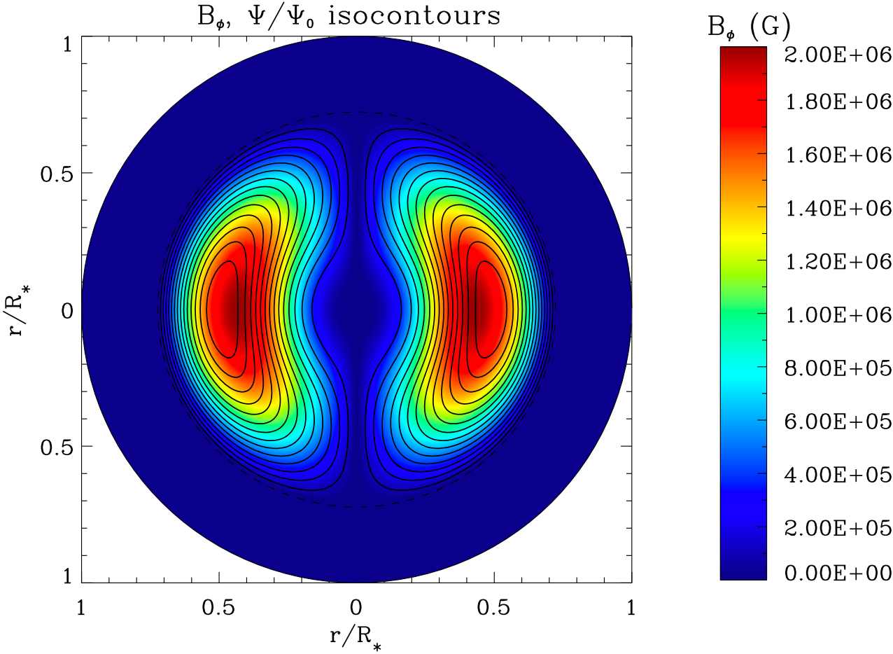
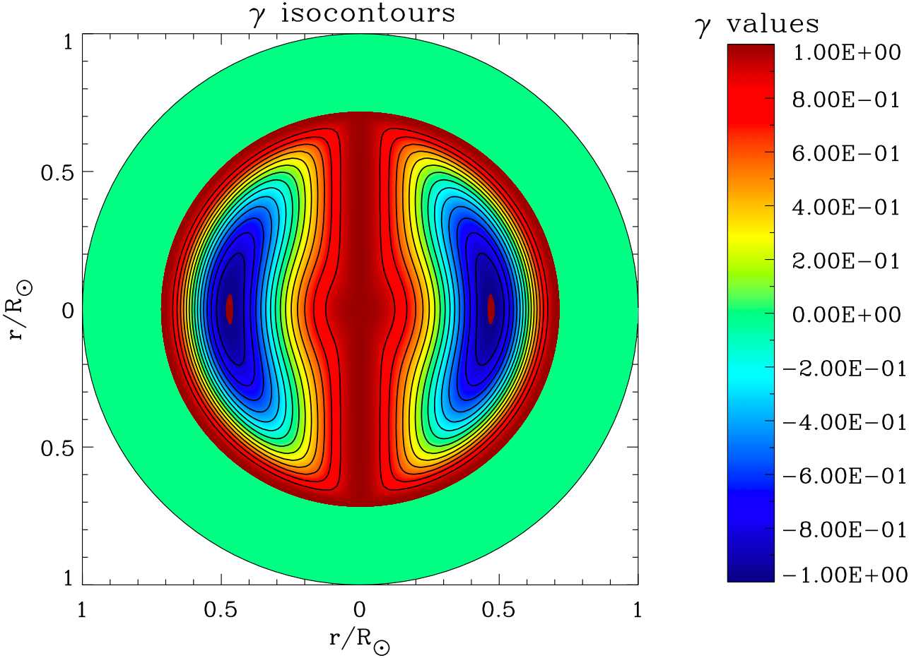
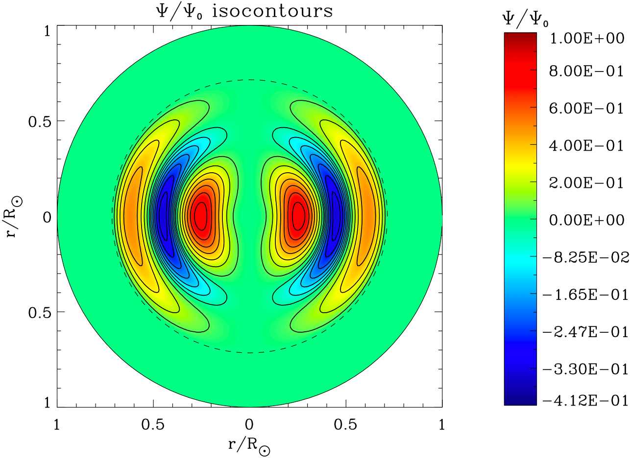
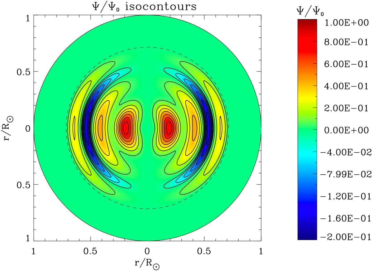
Figure 2: Upper panel: (left) toroidal magnetic field strength in colorscale and normalized isocontours of the poloidal flux function $\Psi$ in meridional cut in the solar case where the field is buried in the radiative core (below $0.726R_{*}$) for the first equilibrium configuration ($\lambda_{1}^{0,1}$); (right) anisotropy factor $\gamma$ (Eq. 88). Lower panel: normalized isocontours of the flux function $\Psi$ in meridional cut (left) for the third possible eigenvalue ($\lambda_{1}^{0,3}$) in the same case, (right) for the fifth possible eigenvalue ($\lambda_{1}^{0,5}$). The dashed circles indicate the radiation-convection limits.

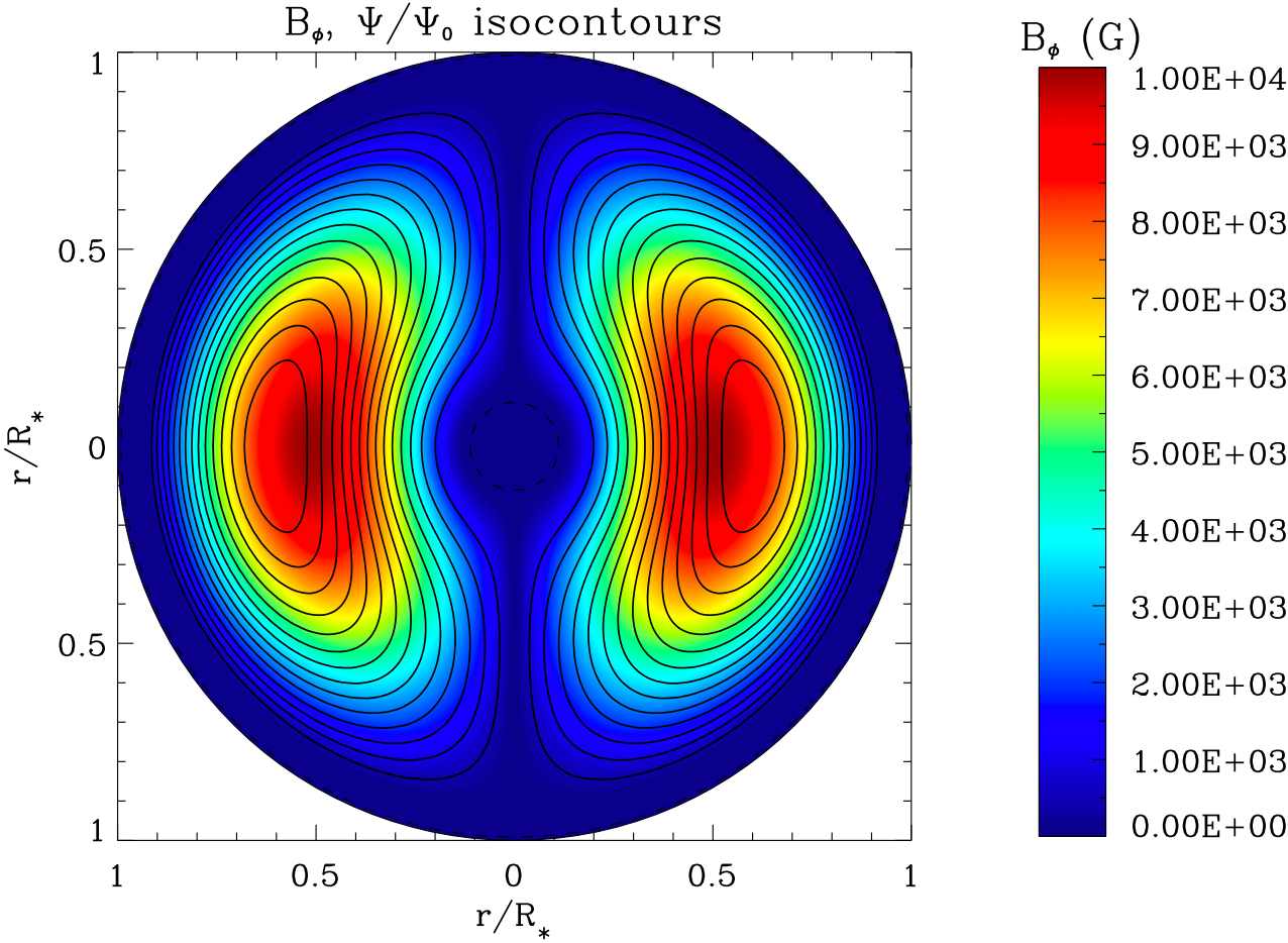
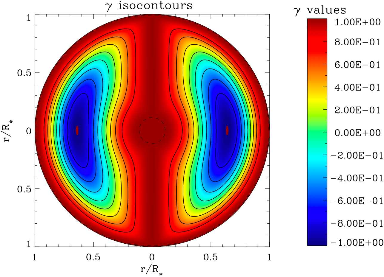
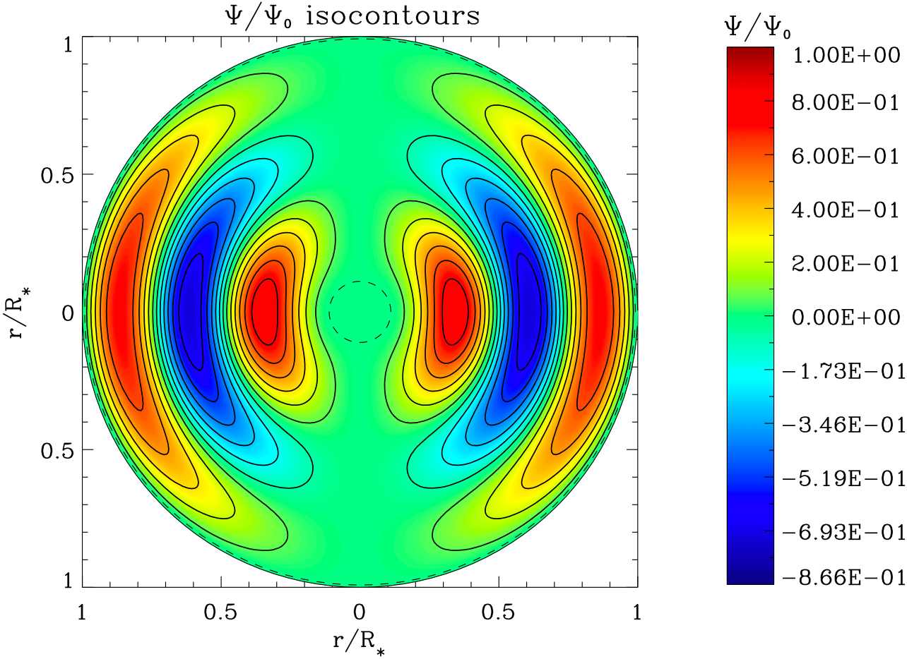
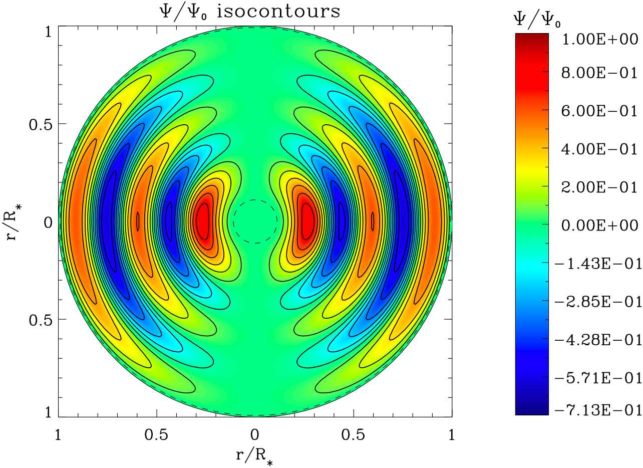
Figure 3: Upper panel: (left) toroidal magnetic field strength in colorscale and normalized isocontours of the poloidal flux function $\Psi$ in meridional cut in the Ap star’s case where the field is confined between $R_{c_{1}}=0.111\>R_{*}$ and $R_{c_{2}}=0.992\>R_{*}$ for the first equilibrium configuration ($\lambda_{1}^{0,1}$); (right) anisotropy factor $\gamma$ (Eq. 88). Lower panel: normalized isocontours of the flux function $\Psi$ in meridional cut (left) for the third possible eigenvalue ($\lambda_{1}^{0,3}$) in the same case, (right) for the fifth possible eigenvalue ($\lambda_{1}^{0,5}$). The dashed circles indicate the radiation-convection limits.

4.2 Fossil fields in early-type stars

Respective corresponding possible configurations in the case of an Ap star are given in Fig. 3.

The model is typical of an A2p-type star, with an initial mass $M_{\rm A}=2.40\,\rm{M}_{\odot}$. The solar metallicity is chosen as the initial one and the model is taken on the ZAMS, its luminosity being $L_{*}=38.0\>\rm{L}_{\odot}$.

Obtained configurations are then mixed poloidal-toroidal (twisted) fields which may be stable in stellar radiation zones (cf. Braithwaite & Spruit 2004; Braithwaite & Nordlund 2006). Their configurations are thus given in both cases by concentric torus, the neutral poloidal points (where $\partial_{r}\Psi=\partial_{\theta}\Psi=0$ so that $B_{r}=B_{\theta}=0$) positions being function of the internal density profile of the star.

Let us emphasize here that the original approach of this work first consists in deriving the Grad-Shafranov-like equation adapted to treat the barotropic magnetohydrostatic equilibrium states for realistic models of stellar interiors. Such approach has already been applied to investigate the internal magnetic configurations in polytropes and in compact objects such that white dwarfs or neutron stars (see e.g. Monaghan 1976; Payne & Melatos 2004; Tomimura & Eriguchi 2005; Yoshida et al. 2006; Haskell et al. 2008; Akgün & Wasserman 2008; Kiuchi & Kotake 2008).

Then, the obtained arbitrary functions are constrained with deriving minimal energy equilibrium configurations for a given conserved mass, azimuthal flux and helicity that generalizes the relaxation Taylor’s states to the self-gravitating case where the field is non-force free.

5 Links between the field’s helicity, topology and energy

5.1 Helicity vs. mixity

Let us express the magnetic field $\left(\bm{B}\right)$ in terms of magnetic stream functions $\xi_{\rm P}$ (for the poloidal component of the field) and $\xi_{\rm T}$ (for its toroidal part):

$$\bm{B}=\bm{\nabla}\times\left[\bm{\nabla}\times\left[\xi_{\rm P}\left(r,\theta\right){\widehat{\bf e}}_{r}\right]+\xi_{\rm T}\left(r,\theta\right){\widehat{\bf e}}_{r}\right].$$ (61)

Next, the vector potential A is given by the relation $\bm{B}=\bm{\nabla}\times\textbf{{A}}$. Knowing that in the confined case the gauge choice is inconsequential, we can identify without further ado

$$\textbf{{A}}=\bm{\nabla}\times\left[\xi_{\rm P}\left(r,\theta\right){\widehat{\bf e}}_{r}\right]+\xi_{\rm T}\left(r,\theta\right){\widehat{\bf e}}_{r}.$$ (62)

The magnetic stream functions are then projected on the spherical harmonics

$$\xi_{\rm P}\left(r,\theta\right) = \sum_{\ell>0}\xi_{0}^{\ell}\left(r\right)Y_{\ell}^{0}\left(\theta\right),$$ (63)

$$\xi_{\rm T}\left(r,\theta\right) = \sum_{\ell>0}\chi_{0}^{\ell}\left(r\right)Y_{\ell}^{0}\left(\theta\right).$$ (64)

From now on, we use Einstein summation convention where $A^{\ell}\>B_{\ell}=\sum_{\ell}A^{\ell}\>B_{\ell}$ and the vectorial spherical harmonics basis $\left({\bf R}_{\ell}^{0}\left(\theta\right),{\bf S}_{\ell}^{0}\left(\theta\right),{\bf T}_{\ell}^{0}\left(\theta\right)\right)$ such that any axisymmetric vector field ${\@vec{u}}(r,\theta)$ can be expanded as

$${\@vec{u}}(r,\theta)=u_{0}^{\ell}(r)\>{\bf R}_{\ell}^{0}\left(\theta\right)+v_{0}^{l}(r)\>{\bf S}_{\ell}^{0}\left(\theta\right)+w_{0}^{\ell}(r)\>{\bf T}_{\ell}^{0}\left(\theta\right),$$ (65)

where the vectorial spherical harmonics ${\bf R}_{\ell}^{0}\left(\theta\right)$, ${\bf S}_{\ell}^{0}\left(\theta\right)$, and ${\bf T}_{\ell}^{0}\left(\theta\right)$ are defined by:

$${\bf R}_{\ell}^{0}\left(\theta\right)=Y_{\ell}^{0}\left(\theta\right)\,\widehat{\bf e}_{r}\hbox{, }{\bf S}_{\ell}^{0}\left(\theta\right)=\bm{\nabla}_{\mathcal{S}}Y_{\ell}^{0}\left(\theta\right)\hbox{, }{\bf T}_{\ell}^{0}\left(\theta\right)=\bm{\nabla}_{\mathcal{S}}\times{\bf R}_{\ell}^{0}\left(\theta\right)\!,$$ (66)

the horizontal gradient being defined as $\bm{\nabla}_{\mathcal{S}}=\mathbf{\hat{e}_{\theta}}\>\partial_{\theta}$. (cf. Rieutord (1987)). Since

$$\bm{\nabla}\times\left(\xi_{\rm P}\,\widehat{\bf e}_{r}\right)=\bm{\nabla}\times\left(\xi_{0}^{\ell}\>Y_{\ell}^{0}\,\widehat{\bf e}_{r}\right)=\bm{\nabla}\times\left(\xi_{0}^{\ell}\>{\bf R}_{\ell}^{0}\right)=\frac{\xi_{0}^{\ell}}{r}{\bf T}_{\ell}^{0},$$ (67)

we get from Eq. (62)

$$\textbf{{A}}=\chi_{0}^{\ell}\>{\bf R}_{\ell}^{0}+\frac{\xi_{0}^{\ell}}{r}{\bf T}_{\ell}^{0}.$$ (68)

On the other hand, we have

$$\bm{B}=\frac{\ell\left(\ell+1\right)}{r^{2}}\xi_{0}^{\ell}\>{\bf R}_{\ell}^{0}+\frac{1}{r}\partial_{r}\xi_{0}^{\ell}\>{\bf S}_{\ell}^{0}+\frac{\chi_{0}^{\ell}}{r}{\bf T}_{\ell}^{0},$$ (69)

from which we finally obtain the expression for the helicity

$$\mathcal{H} = \int_{0}^{R_{*}}\!\!\int_{\Omega}\left\{\left[\chi_{0}^{\ell}\>{\bf R}_{\ell}^{0}+\frac{\xi_{0}^{\ell}}{r}{\bf T}_{\ell}^{0}\right]\cdot\right.$$ (70)

$${\left.\left[\frac{{\ell^{\prime}}\left({\ell^{\prime}}+1\right)}{r^{2}}\xi_{0}^{\ell^{\prime}}\>{\bf R}_{\ell^{\prime}}^{0}+\frac{1}{r}\partial_{r}\xi_{0}^{\ell^{\prime}}\>{\bf S}_{\ell^{\prime}}^{0}+\frac{\chi_{0}^{\ell^{\prime}}}{r}{\bf T}_{\ell^{\prime}}^{0}\right]\right\}}{\rm d}\Omega\,r^{2}{\rm d}r.\qquad$$

At this point, we define a “poloidal helicity” defined by

$$\mathcal{H}_{\rm P}=\int_{\mathcal{V}}\textbf{{A}}_{\rm P}\cdot\bm{B}_{\rm P}\>d{\mathcal{V}}$$ (71)

and a “toroidal helicity” by

$$\mathcal{H}_{\rm T}=\int_{\mathcal{V}}A_{\phi}B_{\phi}\>d{\mathcal{V}}.$$ (72)

Since $\left({\bf R}_{\ell}^{0},{\bf S}_{\ell}^{0},{\bf T}_{\ell}^{0}\right)$ constitutes an orthogonal basis,

$$\int_{\Omega}{\bf R}_{\ell}^{0}\cdot{\bf S}_{\ell}^{0}{\rm d}\Omega=\int_{\Omega}{\bf R}_{\ell}^{0}\cdot{\bf T}_{\ell}^{0}{\rm d}\Omega=\int_{\Omega}{\bf S}_{\ell}^{0}\cdot{\bf T}_{\ell}^{0}{\rm d}\Omega=0,$$ (73)

we get from the previous expression:

$$\mathcal{H} = \int_{0}^{R_{*}}\Bigg{[}\frac{\ell^{{}^{\prime}}\left(\ell^{{}^{\prime}}+1\right)}{r^{2}}\>\chi_{0}^{\ell}\>\xi_{0}^{\ell^{{}^{\prime}}}\int_{\Omega}{\bf R}_{\ell}^{0}\cdot{\bf R}_{\ell^{\prime}}^{0}\>d\Omega$$ (74)

$$+ \frac{1}{r^{2}}\>\xi_{0}^{\ell}\>\chi_{0}^{\ell^{\prime}}\int_{\Omega}{\bf T}_{\ell}^{0}\cdot{\bf T}_{\ell^{\prime}}^{0}\>d\Omega\Bigg{]}\,r^{2}{\rm d}r$$

and we verify that

$$\mathcal{H}=\mathcal{H}_{\rm P}+\mathcal{H}_{\rm T}.$$ (75)

From this expression (74) we can draw two conclusions:

1. A magnetic field has to be mixed (both poloidal and toroidal) to be helical;

2. The poloidal and the toroidal helicities are equal. This can be verified, exploiting the orthogonality relations

   $$\int_{\Omega}{\bf R}_{\ell}^{0}\cdot{\bf R}_{\ell^{\prime}}^{0}\>d\Omega=\delta_{\ell,\ell^{\prime}}$$ (76)

   and

   $$\int_{\Omega}{\bf T}_{\ell}^{0}\cdot{\bf T}_{\ell^{\prime}}^{0}\>d\Omega=\ell\left(\ell+1\right)\delta_{\ell,\ell^{\prime}},$$ (77)

   $\delta_{\ell,\ell^{\prime}}$ being the usual Kronecker symbol. Then, we get

   $$\mathcal{H}_{\rm P}=\mathcal{H}_{\rm T}=\ell\left(\ell+1\right)\int_{0}^{R_{*}}\xi_{0}^{\ell}\>\chi_{0}^{\ell}\>dr=\mathcal{H}/2.$$ (78)

5.2 Helicity vs. energy

Now, we focus back again on the helicity expression in terms of the poloidal flux function $\Psi$. The equations (55) and (56) are rewritten as

$$\bm{B}_{\rm P} = \frac{R}{\lambda_{1}^{0,i}}\bm{\nabla}\times\bm{B}_{\rm T},$$ (79)

$$\bm{B}_{\rm T} = \frac{R}{\lambda_{1}^{0,i}}\bm{\nabla}\times\bm{B}_{\rm P}-\frac{R}{\lambda_{1}^{0,i}}\>\mu_{0}\>\beta_{0}\>{\overline{\rho}}\>r^{2}\>\sin\theta\>\mathbf{\hat{e}_{\varphi}}$$ (80)

$$= \frac{R}{\lambda_{1}^{0,i}}\bm{\nabla}\times\left[\bm{B}_{\rm P}-\mu_{0}\>\beta_{0}\>{\overline{\rho}}\>r^{2}\>\cos\theta\>\mathbf{\hat{e}_{r}}\right].$$

We thus obtain the two vector potentials

$$\textbf{{A}}_{\rm P} = \frac{R}{\lambda_{1}^{0,i}}\left(\bm{B}_{\rm P}-\mu_{0}\>\beta_{0}\>{\overline{\rho}}\>r^{2}\>\cos\theta\>\mathbf{\hat{e}_{r}}\right)+\bm{\nabla}\Lambda_{\rm P},$$ (81)

$$\textbf{{A}}_{\rm T} = \frac{R}{\lambda_{1}^{0,i}}\bm{B}_{\rm T}+\bm{\nabla}\Lambda_{\rm T},$$ (82)

$\Lambda_{\rm P}$ and $\Lambda_{\rm T}$ being scalar gauge fields left free. When deriving the poloidal and toroidal helicities with the boundary condition $\bm{B}\cdot{\widehat{\bf e}}_{r}=0$ at the surface, these ones disappear after integration and we find :

$${\mathcal{H}}_{\rm P} = \frac{2\>\mu_{0}\>R}{\lambda_{1}^{0,i}}\int_{\mathcal{V}}\frac{\bm{B}_{\rm P}^{2}}{2\>\mu_{0}}\>d{\mathcal{V}}-\frac{\mu_{0}\>R}{\lambda_{1}^{0,i}}\beta_{0}\>\int_{\mathcal{V}}{\overline{\rho}}\>\Psi\>d{\mathcal{V}},$$ (83)

$${\mathcal{H}}_{\rm T} = \frac{2\>\mu_{0}\>R}{\lambda_{1}^{0,i}}\int_{\mathcal{V}}\frac{\bm{B}_{\rm T}^{2}}{2\>\mu_{0}}\>d{\mathcal{V}}.$$ (84)

So, introducing the poloidal and toroidal magnetic energies ${U}_{\rm mag;P}=\int_{\mathcal{V}}\frac{\bm{B}_{\rm P}^{2}}{2\>\mu_{0}}\>{\rm d}{\mathcal{V}}$ and ${U}_{\rm mag;T}=\int_{\mathcal{V}}\frac{\bm{B}_{\rm T}^{2}}{2\>\mu_{0}}\>{\rm d}{\mathcal{V}}$ (respectively), we obtain:

$${\mathcal{H}}_{\rm P}=\frac{2\>\mu_{0}\>R}{\lambda_{1}^{0,i}}\left({U}_{\rm mag;P}-\frac{1}{2}\beta_{0}M_{\Psi}\right),$$ (85)

where we identify $M_{\Psi}=\mathcal{I}_{I;1}=\int_{\mathcal{V}}{\overline{\rho}}\>\Psi\>d{\mathcal{V}}$, and

$${\mathcal{H}}_{\rm T}=\frac{2\>\mu_{0}\>R}{\lambda_{1}^{0,i}}{U}_{\rm mag;T}.$$ (86)

Finally, adding these two last equations, we get the global relation between the helicity and the magnetic energy in the non force-free case

$${\mathcal{H}}=\frac{2\>\mu_{0}\>R}{\lambda_{1}^{0,i}}\left({U}_{\rm mag}-\frac{1}{2}\>\beta_{0}M_{\Psi}\right),$$ (87)

where we recognize in the second term the non force-free contribution, which is the first invariant: the mass enclosed in magnetic flux surface.

5.3 Helicity vs. topology

The $l>1$ latitudinal modes contributions

As shown by Broderick & Narayan (2008) for a set of modes $l$ ranging from 1 to 8 in the case of force-free solutions applied in an incompressible media, the first dipolar eigenvalue $\lambda_{1}^{0,1}$ corresponds to the minimum energy configuration. Furthermore, from the Eq. (87), it arises directly that adding contributions from the higher multipolar components of the field (force-free) will result in adding a positive amount of magnetic energy to the total energy, and this one will not be the minimal state.

Lowest energy radial mode

We plotted in Figure 4a and 4b the poloidal, toroidal and total helicity in the case of the Sun and of the Ap star. It clearly stems from this figure that the poloidal and the toroidal helicities are equal (cf. Eq. 78) for the eigenvalues given in Tab 1 (represented by red diamonds). Moreover, the energy of the poloidal component of the field ($U_{\rm mag;P}$) can be compared to the one correponding to the toroidal part ($U_{\rm mag;T}$) and we see that they are of the same order of magnitude.

In Figure 5a and 5b are represented the ratios $\mathcal{E}_{\rm mag}/\mathcal{H}$ for the poloidal, toroidal and global contributions, with and without the non force-free term, as a function of the parameter $\lambda_{1}^{0,i}$ respectively in the case of the Sun and of the Ap type star. The first dipolar eigenvalue $\lambda_{1}^{0,1}$ present the minimum energy compared with highest radial modes. It is thus the most probable configuration achieved after relaxation and from now on we focus on it.

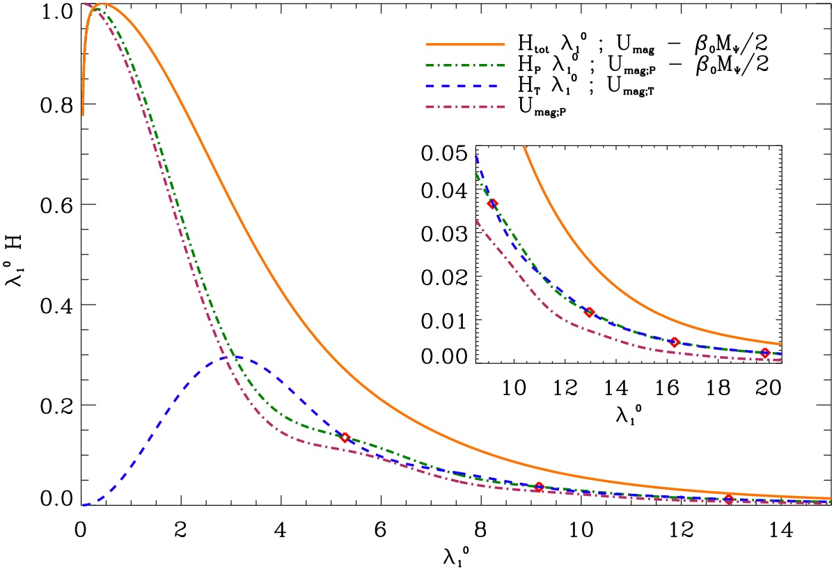
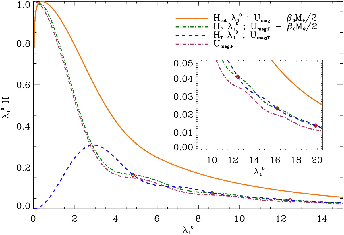
Figure 4: Normalized total, poloidal, and toroidal helicities as a function of the eigenvalue ($\lambda_{1}^{0}$) in the case (a, top) of the young Sun and (b, bottom) of the studied Ap star. The red diamonds represent the eigenvalues ($\lambda_{1}^{0,i}$) given in Tab 1 for which Eq. (78) is verified. Using Eq. (86), we directly deduce $U_{\rm mag;T}$ while $U_{\rm mag;P}$ is given in purple.

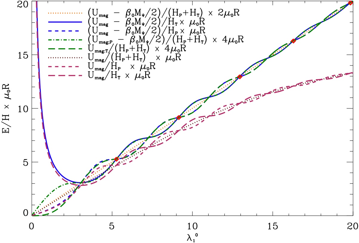
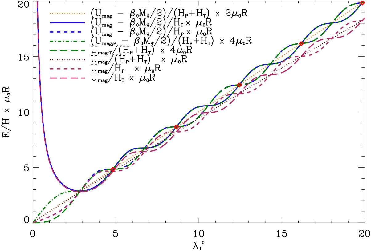
Figure 5: Magnetic energy/helicity ratios for the total, poloidal, and toroidal contributions as a function of the eigenvalue ($\lambda_{1}^{0}$) with (first five curves) and without (last three curves) the non-force-free term in the case (a, top) of the young Sun and (b, bottom) of the studied Ap star. For the eigenvalues ($\lambda_{1}^{0,i}$) represented by the red diamonds (cf. Tab 1), Eqs. (78,87,85,86) are simultaneously verified.

6 Discussion

6.1 Stability criteria

First, it is interesting to examine the ratio of the field’s poloidal component amplitude with its toroidal one. Then, we define the anisotropy factor ($\gamma$) of the configuration by

$$\gamma\left(r,\theta\right)=\frac{B_{\rm P}^{2}-B_{\rm T}^{2}}{B_{\rm P}^{2}+B_{\rm T}^{2}},\,\,\,\hbox{where}\,\,\,B_{\rm P}=\sqrt{B_{r}^{2}+B_{\theta}^{2}}\,.$$ (88)

It runs between -1 when the field is completely toroidal to 1 when it is completely poloidal. In Figs. 2 & 3, it is shown for the first configurations obtained in the solar and in the Ap star cases. In both ones, the field is strongly toroidal $(\gamma\approx-1)$ in the center of the torus, which corresponds to the neutral point of the poloidal field (where we recall that $\partial_{r}\Psi=\partial_{\theta}\Psi=0$), while it is strongly poloidal $(\gamma\approx 1)$ around the magnetic axis of the star where the toroidal field is weak. Between those two regimes, both components have comparable strengths where $\gamma\approx 0$. Then, proposed configurations may be stable since poloidal and toroidal fields can stabilize each other respectively (Wright 1973; Tayler 1980; Braithwaite 2009). The complete stability analysis following the analytical method given in Bernstein et al. (1958) and using 3D numerical simulations will be achieved in a near future.

6.2 Comparison to numerical simulations

Next, let us compare in more details our analytical configuration to those obtained using numerical simulations (see Braithwaite & Spruit (2004); Braithwaite & Nordlund (2006); Braithwaite (2008)).

Braithwaite and collaborators performed numerical magnetohydrodynamical simulations of the relaxation of an initially random magnetic field in a stably stratified star. Then, this initial magnetic field is always found to relax on the Alfvén time-scale into a stable magneto-hydrostatic equilibrium mixed configuration consisting of twisted flux tube(s). Two families are then identified: in the first one, the equilibria configurations are roughly axisymmetric with one flux tube forming a circle around the equator such as our configuration; in the second family, the relaxed fields are non-axisymmetric consisting of one or more flux tubes forming a complex structure with their axis lying at roughly constant depth under the surface of the star. Whether an axisymmetric or non-axisymmetric equilibrium forms depends on the initial condition chosen for the radial profile of the initial stochastic field strength $|{\textbf{{B}}}||\propto{\overline{\rho}}^{p}$: a centrally concentrated one evolves into an axisymmetric equilibrium as in our configuration while a more spread-out field with a stronger connection to the atmosphere relaxes into a non-axisymmetric one. Braithwaite (2008) indicates that, using an ideal-gas star modelled initially with a polytrope of index $n=3$, the threshold is $p\approx 1/2$.

Moreover, as shown in Fig. 7 in Braithwaite (2008), a selective decay of the total helicity (${\mathcal{H}}$) and of the magnetic energy ($U_{\rm Mag}$) occurs during the initial relaxation with a stronger decrease of $U_{\rm Mag}$ than that of ${\mathcal{H}}$. This hierarchy well known in plasma physics (see for example Biskamp (1997) and Shaikh et al. (2008)) justifies the variational method used to derive our configuration (Montgomery & Phillips (1988)) while the introduction of ${\mathcal{I}}_{{\rm I};1}$ is justified by the non force-free character of the field in stellar interiors (Reisenegger 2009) and by the stratification which inhibits the transport of flux and mass in the radial direction (see §3.2. and Braithwaite (2008)).

Finally, note that our analytical configuration for which $U_{\rm mag;P}/U_{\rm mag}\approx 0.45$ verifies the stability criterion derived by Braithwaite (2009) for axisymmetric configurations:

$${\mathcal{A}}\frac{U_{\rm mag}}{U_{\rm grav}}<\frac{U_{\rm mag;P}}{U_{\rm mag}}\leq 0.8,$$ (89)

where $U_{\rm grav}$ is the gravitational energy in the star and ${\mathcal{A}}$ a dimensionless factor whose value is of order $10$ in a main-sequence star and of order $10^{3}$ in a neutron star while we expect $U_{\rm mag}/U_{\rm grav}<10^{-6}$ in a realistic star (see for example Duez et al. (2010)).

Our analytical solution is thus similar to the axisymmetric non force-free relaxed solutions family obtained by Braithwaite & Spruit (2004) and Braithwaite & Nordlund (2006).

Those types of configurations can thus be relevant to model initial equilibrium conditions for evolutionary calculations involving large-scale fossil fields in stellar radiation zones. First, they can be used to initiate MHD rotational transport in dynamical stellar evolution codes where it is implemented (cf. Mathis & Zahn 2005) . There, axisymmetric transport equations have been derived to study the secular dynamics of the mean axisymmetric component of the magnetic field, the magnetic instabilities being treated using phenomenological prescriptions (Spruit 1999, 2002; Maeder & Meynet 2004) that have to be verified and improved by numerical experiments (Nordlund (2006) and subsequent works; Zahn et al. (2007); Gellert et al. (2008)). On the other hand, those can also be used as initial conditions for large-scale numerical simulations of stellar radiation zones (Garaud 2002; Brun & Zahn 2006).

6.3 Relaxed configurations and boundary conditions

Let us now discuss the boundary conditions we choosed. Since equilibrium states are known to minimize the energy/helicity ratio, we follow the procedure established by Chandrasekhar & Prendergast (1958) and Woltjer (1959b) to constrain the arbitrary functions of the magnetohydrostatic equilibrium. This procedure, which minimizes the energy with respect to given invariants of the system (and in particular the helicity), assumes the following boundary condition $\bm{B}\cdot\mathbf{\hat{e}_{r}}=0$ that leads to an azimuthal current sheet due to the non-zero latitudinal field at the upper boundary ($B_{\theta}\left(R_{\rm sup},\theta\right)\neq 0$). This is a potential source of instability and in the case of our configuration we have to evaluate its effect on the stability (cf. Bellan 2000).

Next, in a stellar context, we have to allow open configurations as observed and thus to match the internal solution with an external multipolar one. It remains then to be seen whether the invariants are conserved, as they are in the confined case (Dixon et al. 1989).

Finally, independently from the chosen type of configuration (confined or matched with a multipolar external field), we have to search solutions that allow the continuity of the magnetic field and of the associated currents at the boundaries to cancel the possible induced instabilities. This leads to an ill-posed problem which must be solved in a subtle way (see Monaghan 1976; Lyutikov 2009). In the present state of art, no solution has been derived that both minimizes the energy/helicity ratio and satisfies this type of surface boundary conditions. This will be the next step and it is out of the scope of the present paper.

7 Conclusion

In the context of improving stellar models by taking into account in the most consistent way as possible dynamical processes such as rotation and magnetic field, we examine possible magnetic equilibrium configurations to model initial fossil fields.

We generalize the pioneer work by Prendergast (1956) in deriving the barotropic magnetohydrostatic equilibrium states of realistic stellar interiors which are a first equilibrium family. These will then evolve due to other dynamical processes such as Ohmic diffusion, differential rotation, meridional circulation, and turbulence. Relaxed minimum energy equilibrium configurations are then obtained for a given conserved mass and helicity that correspond to the Taylor’s relaxation states in the self-gravitating non force-free case. These are then applied to the internal radiation zone of the young Sun and to the radiative interior of an Ap star on the ZAMS. Mixed poloidal and toroidal magnetic configurations, potentially stable in stellar radiation zones, are obtained.

Now, we have thus to study the stability of these magnetic topologies. Moreover, the case of general baroclinic equilibrium states have to be studied (Paper II).

These equilibrium configurations have then to be used as possible initial conditions for rotational transport processes in stellar radiative regions that will allow to study internal stellar MHD over secular time-scales.