Decomposition and Model Selection for Large Contingency Tables

Abstract

Large contingency tables summarizing categorical variables arise in many areas. One example is in biology, where large numbers of biomarkers are cross-tabulated according to their discrete expression level. Interactions of the variables are of great interest and are generally studied with log-linear models. The structure of a log-linear model can be visually represented by a graph from which the conditional independence structure can then be easily read off. However, since the number of parameters in a saturated model grows exponentially in the number of variables, this generally comes with a heavy computational burden. Even if we restrict ourselves to models of lower order interactions or other sparse structures we are faced with the problem of a large number of cells which plays the role of sample size. This is in sharp contrast to high-dimensional regression or classification procedures because, in addition to a high-dimensional parameter, we also have to deal with the analogue of a huge sample size. Furthermore, high-dimensional tables naturally feature a large number of sampling zeros which often leads to the nonexistence of the maximum likelihood estimate. We therefore present a decomposition approach, where we first divide the problem into several lower-dimensional problems and then combine these to form a global solution. Our methodology is computationally feasible for log-linear interaction models with many categorical variables each or some of them having many levels. We demonstrate the proposed method on simulated data and apply it to a bio-medical problem in cancer research.

1 Background

We consider the problem of estimation and model selection in log-linear models for large contingency tables involving many categorical variables. This problem encompasses the estimation of the graphical model structure for categorical variables. This structure learning task has lately received considerable attention as it plays an important role in a broad range of applications. The conditional independence structure of the distribution can be read off directly from the structure of a graphical model (a graph) and hence provides a graphical representation of the distribution that is easy to interpret (see Lauritzen (1996)). Graphical models for categorical variables correspond to a class of hierarchical log-linear interaction models for contingency tables. Thus, fitting a graph corresponds to model selection in a hierarchical log-linear model $\log({\bf p})=\mathbf{X}\boldsymbol{\beta}$, where $\bf p$ is the vector of cell probabilities of a table, $\boldsymbol{\beta}$ is a parameter vector and $\mathbf{X}$ is the design matrix (see section 2.2).

Fitting the log-linear model for large contingency tables in full detail turns out to be a very hard computational problem in practice. In the following, we list three possible goals for fitting log-linear models. The goals are ranked in increasing order according to their computational difficulty:

Graphical Structure

Finding the graphical structure for discrete categorical variables is easiest but it doesn’t allow to infer the magnitude of the coefficients $\boldsymbol{\beta}$ in the log-linear model, see also formula (3).

Parameter Vector $\boldsymbol{\beta}$

The next level of difficulty is the estimation of the unknown parameter vector $\boldsymbol{\beta}$ in a log-linear model whose full dimension equals the number of cells in the contingency table. For large tables, the dimension of $\boldsymbol{\beta}$ is huge but under some sparsity assumptions it is possible to accurately estimate such a high-dimensional vector using suitable regularisation. The major problem is here that besides the high-dimensionality of $\boldsymbol{\beta}$, the analogue of the sample size (the row-dimension of $\mathbf{X}$) is huge, e.g. $3^{40}$ for 40 categorical variables having 3 levels each.

Probability Vector ${\bf p}$

The most difficult problem is the estimation of the probability vector ${\bf p}$ whose dimension equals again the number of cells in the table. It is rather unrealistic to place some sparsity assumptions on ${\bf p}$ in the sense that many entries would equal exactly zero which would enable feasible computation. Therefore, it is impossible to ever compute an estimate of the whole probability vector ${\bf p}$ (e.g. having dimensionality $3^{40}$). Nevertheless, thanks to sparsity of the parameter vector $\boldsymbol{\beta}$ and the junction tree algorithm, it is possible to compute accurate estimates $\{\hat{\bf p}(i);\ i\in{\cal C}\}$ for any reasonable-sized collection ${\cal C}$ of cells in the contingency table.

There is hardly any method which can achieve all these goals for contingency tables involving many, say more than 20, variables. One approach to address the log-linear modeling problem for large contingency tables is presented in Jackson et al. (2007), where some dimensionality reduction is achieved by reducing the number of levels per variable. The reduction is accomplished via collapsing two categories by aggregating their counts if the two categories behave sufficiently similar. If $d$ variables are considered, this method reduces the problem at best to $d$ binary variables. For this special case with binary factors, an approach based on many logistic regressions can be used for fitting log-linear interaction models whose computational complexity is feasible even if the number of variables is large (Wainwright et al., 2007). Another method to address the log-linear modeling problem for large contingency tables is proposed in Kim (2005), where the variables are grouped such that they are highly connected within groups but less between groups and graphical models are fitted for these subgroups. The subgraph models are then combined using so-called graphs of prime separators. The implementation of the combination however is not an easy task and no exact algorithm is given on how to combine the models.

Our presented methodology allows to achieve all the goals above for categorical variables having possibly different numbers of levels: inference of a graphical model for discrete variables, of a sparse parameter vector in a log-linear model and of a collection of cell probabilities. Motivated by the approach in Kim (2005), we also propose a decomposition approach, where the dimensionality reduction is achieved by recursively collapsing the large contingency table on certain variables (decomposition) and thereby reducing the problem to smaller tables which can be handled more easily. All the fitted lower-dimensional log-linear models are combined appropriately to represent an estimation of the joint distribution of all variables. The procedure enables us to handle very large tables e.g. up to hundreds of categorical variables, where some or all of them can have more than two categories. This multi-category framework is much more challenging than the approach in Wainwright et al. (2007) for large binary tables. In Ravikumar et al. (2009), an extension to the multi-category case within the class of pairwise Markov random fields is sketched: it is argued that higher-order interactions could be included in a pairwise Markov field but no methodology or algorithm is described how to actually do this difficult computational task.

2 Definitions

In this section, we introduce several important theoretical concepts. First, we define the general log-linear interaction model. Subsequently, we introduce the hierarchical log-linear model and the graphical model as restricted versions of the log-linear interaction model. Then, we define collapsibility and decomposability, which are crucial concepts for breaking up a graphical model into smaller pieces.

2.1 Log-linear interaction model

We adopt here the notation of Darroch et al. (1980). Assume we have some factors or categorical variables, indexed by a set $V$. Each factor $v\in V$ has a set of possible levels $I_{v}=\{0,1,\ldots,k_{v}\}$. The contingency table is the cartesian product of the individual sets: $I=\prod_{v\in V}I_{v}$. An individual cell in the contingency table is denoted by $i\in I$ and the corresponding cell count by $n_{i}$. A marginal index for variable set $a\subseteq V$ is denoted by $i_{a}$. For example, assume we have two binary variables, then $V=\{1,2\}$, $I_{1}=I_{2}=\{0,1\}$ and the contingency table is given by $I=\{(0,0),(0,1),(1,0),(1,1)\}$. An individual cell is for example $i=(0,1)$ and the index describing the margin along the second variable ($a=2$) is $i_{a}=i_{2}=(1)$. The total number of cells in a contingency table is $m=|I|=\prod_{v\in V}|I_{v}|$. In our example, $m=4$. A natural way of representing the distribution of the cell counts is via a vector of probabilities $\mathbf{p}=(p(i),i\in I)$. In our example, this would correspond to defining four probabilities $\mathbf{p}=(p_{(0,0)},p_{(0,1)},p_{(1,0)},p_{(1,1)})$. If a total number of $n$ individuals are classified independently, then the distribution of the corresponding cell counts $\mathbf{n}=(n_{1},n_{2},\ldots,n_{m})$ is multinomial with probability $\mathbf{p}$. Finally, the general log-linear interaction model specifies the unknown distribution $\mathbf{p}$ as follows:

$$\log p(i)=\sum_{a\subseteq V}\xi_{a}(i_{a})\quad\forall i\in I$$ (1)

where $\xi_{a}$ are functions of cell $i$ which only depend on the variables in $a$. These functions are called interactions between the variables in $a$. If $|a|=1$, $\xi_{a}$ is called main effect, if $|a|=2$ first order interaction and an interaction of order $k-1$ if $|a|=k$. For identifiability purposes we impose constraints on the functions, namely that $k^{th}$-order interaction functions are orthogonal to interaction functions of lower order.

2.2 Hierarchical log-linear models

A hierarchical log-linear model is a log-linear interaction model with the additional constraint, that a vanishing interaction forces all interactions of higher order to be zero as well:

$$\xi_{a}=0\Longrightarrow\xi_{b}=0\quad\forall\ a\subseteq b\subseteq V$$

Hierarchical models can be specified via the so-called generators or generating class $\mathcal{G}$ which is a set of subsets of $V$ consisting of the maximal interactions which are present. More precisely, the generating class $\mathcal{G}$ has the following property:

$$\xi_{a}=0\Longleftrightarrow\textrm{ there is no }q\in\mathcal{G}\textrm{ with }a\subseteq q.$$ (2)

Consider an example with three binary factors. An example for a hierarchical log-linear model is the model consisting of all main effects, an interaction between $1$ and $2$ and an interaction between $1$ and $3$: this corresponds to $\mathcal{G}=\{\{1,2\},\{1,3\}\}$. However, the log-linear interaction model with main effect $1$ and interaction between $1$ and $2$ (but no main effect $2$) is not in the class of hierarchical log-linear models.

If we go back to formula (1) and rewrite it in matrix formulation, we get:

$$\log{(\mathbf{p})}=\mathbf{X}\boldsymbol{\beta},$$ (3)

where $\boldsymbol{\beta}$ is a vector of unknown coefficients and $\mathbf{X}\in\mathbb{R}^{m\times m}$ the design matrix. Each row of $\mathbf{X}$ corresponds to a certain cell and the columns of $\mathbf{X}$ correspond to the functions $\xi_{a}(i_{a})$. The number of columns needed to represent the function $\xi_{a}$ depends on the number of different states $i_{a}$ can take on. For example consider a categorical variable $a$ that can take on 3 levels. Then, $\xi_{a}$ is called a main effect (as $|a|=1$) and $X_{a}$ (the columns of $\mathbf{X}$ corresponding to $a$) is 2-dimensional. Originally, it would be 3-dimensional but for identifiability purposes, the subspace spanned by $X_{a}$ is chosen orthogonal to the already existing columns of lower order interaction (here orthogonal to the intercept) and we further choose it orthogonal within the subspace. By choosing the identifiability constraints this way, the parameterization of the matrix used in (3) is equivalent to choosing a poly contrast in terms of ANOVA. If we go back to our example with two binary factors where $m=4$, (3) becomes:

$$\log{\mathbf{p}}\begin{pmatrix}(0,0)\\ (0,1)\\ (1,0)\\ (1,1)\end{pmatrix}=\mathbf{X}\boldsymbol{\beta},\phantom{blasd}$$

(4)

$$\textrm{ with }\mathbf{X}=\begin{pmatrix}1&\phantom{-}1&\phantom{-}1&-1\\ 1&\phantom{-}1&-1&\phantom{-}1\\ 1&-1&\phantom{-}1&-1\\ 1&-1&-1&\phantom{-}1\end{pmatrix},\textrm{ and }\boldsymbol{\beta}=(\beta_{\emptyset},\beta_{1},\beta_{2},\beta_{12})^{T},$$

where the first column is the intercept and belongs to $a=\emptyset$, the second column belongs to $a=1$ and has entry 1 whenever variable $a=1$ takes on the first level and -1 else and similarly for the third column. The fourth column belongs to the interaction between variable 1 and 2. A description of $\mathbf{X}$ for the general case can be found in Dahinden et al. (2007). In the following we will denote the components of $\boldsymbol{\beta}$ belonging to $X_{a}$ with $\beta_{a}$.

2.3 Graphical models

We first introduce some terminology. A graph is defined as a pair $G=(V,E)$, where $V$ is the set of vertices or nodes and $E\subseteq V\times V$ is the set of edges linking the vertices. Each node represents a (categorical) random variable. Here we only consider undirected graphs which means that $(u,v)\in E$ is equivalent to $(v,u)\in E$. A path from $u$ to $v$ is a sequence of distinct nodes $v_{0}=u,v_{1},\ldots,v_{n}=v\textrm{ such that }(v_{i},v_{i+1})\in E$ for all $i\in\{0,1,\ldots,n-1\}$. Given three sets of variables $A,S,B\subseteq V$, we say that $S$ separates $A$ from $B$ in $V$ if all paths from vertices in $A$ to vertices in $B$ have to pass through $S$. Consider a random vector $\mathbf{Z}=\{Z_{v},v\in V\}$ with a given distribution. We say that the distribution of $\mathbf{Z}$ is globally Markov with respect to a graph $G$ if for any 3 disjoint subsets $A,S,B\subseteq V$ the following property holds:

$$S\textrm{ separates }A\textrm{ from }B\Longrightarrow Z_{A}\bot Z_{B}|Z_{S},$$ (5)

where the symbol “$\bot$” denotes (conditional) independence. This states that we can read off conditional independence relations directly from the graph if the distribution is globally Markov with respect to the graph. Graphical models therefore provide a way to represent conditional (in)dependence relations between variables in terms of a graph structure. We say that a set of nodes of $G$ forms a complete subgraph of $G$ if every pair in that set is connected by an edge. A maximal complete subgraph is called a clique.

The undirected graphical model (from now on “graphical model” for short) represented by a graph $G$ corresponds to a hierarchical log-linear model where the cliques of the graph are the generators of the model. If we go back to our example in the previous section and assume that $\beta_{12}\neq 0$ in formula (LABEL:beispiel), then the hierarchical log-linear model (LABEL:beispiel) can be represented by the graphical model in Fig. 1(a); if $\beta_{12}=0$, then the corresponding graphical model is the one in Fig. 1(b).

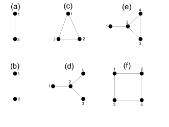
Figure 1: Examples of graphical models. (a) Full (maximal) model corresponding to the example given by formula (LABEL:beispiel). (b) In the same example graph with $\beta_{12}=0$. (c) Example of an interaction graph corresponding to a hierarchical log-linear model which is not graphical. (d) The separator $S=2$ has index $\nu(S)=2$. (e) The separator $S=2$ has index $\nu(S)=1$.

Conversely, assume that the generators of a log-linear model are given by a set $\mathcal{G}$. By connecting all the vertices appearing in the same generator with each other and placing no other edge, the so-called interaction graph is built. By the definition of the interaction graph and by looking at formula (1), it becomes clear that the distribution induced by the log-linear model is Markov with respect to the interaction graph and we can read off conditional independencies directly from the graph. It is also clear that $\mathcal{G}$ corresponds to a graphical model via its interaction graph if and only if $\mathcal{G}$ is the set of cliques of this graph. In that case we say that $\mathcal{G}$ is a graphical generating class. If there are cliques in the interaction graph which are not in $\mathcal{G}$, the hierarchical log-linear interaction model is not graphical and its interaction structure cannot be adequately represented by the graph alone. However, the graph may still completely represent all conditional independencies of the underlying distribution. The simplest example of a hierarchical log-linear model $M$ which is not graphical is $V=\{1,2,3\}$ and $\mathcal{G}=\{\{1,2\},\{2,3\},\{3,1\}\}$. Its interaction graph is shown in Fig. 1(c) which has as its only clique the complete graph $\{1,2,3\}$. Since the set of cliques and the set of generators $\mathcal{G}$ are not identical, model $M$ is not graphical.

Any joint probability distribution of discrete random variables can be expanded in terms of a log-linear interaction model. For some distributions it is possible to represent all (conditional) independencies in an undirected graphical model and these distributions are called faithful to their interaction graph $G$ or we say that the graph is a perfect map of the distribution. In other words, the graph captures all and only the conditional independence relations of the distribution.

2.4 Collapsibility

Collapsing over a variable simply means summing over that variable and thereby reducing (collapsing) the table to the remaining dimensions.

When collapsing over a variable, spurious associations between the remaining variables may be introduced and original associations can vanish. A criterion that addresses this problem is collapsibility. We say that a variable is collapsible with respect to a specific interaction $\xi_{a}$, when the interaction in the original contingency table is identical to the interaction in the collapsed contingency table (i.e., $\xi_{a}$ in equation (1) remains the same).
The general result regarding collapsibility, which goes back to a theorem stated in Bishop et al. (1975), can be summarized as follows:

$$\textrm{ By collapsing a table over a variable which interacts with }s\textrm{ other variables, then }s\textrm{- and higher}$$

order interactions between the remaining variables are not changed in the collapsed table. (6)

Conversely, lower-order interactions between the remaining variables are affected by collapsing.

Suppose, for example, that variable $X$ only interacts with one other variable $Y$. If we collapse over $X$, no interaction changes but main effects may be changed. Furthermore, suppose that $Z$ is independent of all other variables. Then neither main effects nor interactions change when collapsing over $Z$.

2.5 Decomposability

Assume a graphical model on the vertex set $V$. A triple of disjoint subsets $(A,S,B)$ of the vertex set $V$ forms a decomposition if (i) $V=A\cup S\cup B$, (ii) $S$ separates $A$ from $B$ and (iii) $S$ is complete.

Decomposability is defined recursively: A graph is decomposable if it is complete or if there exists a decomposition $(A,S,B)$ where the subgraphs of $G$ restricted to the vertex sets $A\cup S$ and $S\cup B$ are decomposable.

Denote by $\mathcal{C}$ the set of all cliques of a decomposable graph and by $\mathcal{S}$ the set of all separators. For a decomposable graph with decomposition into cliques $\mathcal{C}$ and separators $\mathcal{S}$, the probability of a cell $i$ is given by the following formula (see for example Proposition 4.18 of Lauritzen (1996)):

$$p(i)=\frac{\prod_{C\in\mathcal{C}}p(i_{C})}{\prod_{S\in\mathcal{S}}p(i_{S})^{\nu(S)}},$$ (7)

where $\nu(S)$ is the so-called index of the separator. The formal definition of the index $\nu(S)$ is a bit cumbersome and is given in Lauritzen (1996). However, intuitively it can be thought of as the number of times the set $S$ acts as a separator. For example: In Fig. 1(d), node $2$ separates $\{1\}$ and $\{4\}$ (the cliques consisting of single nodes $\{1\}$ and $\{4\}$), $\{1\}$ and $\{3\}$, and also $\{3\}$ and $\{4\}$. Therefore the index of the separating node $2$ is 3, as node 2 acts three times as separator. If we look at Fig. 1(e), we see that the node $2$ only separates $\{1\}$ from the clique $\{3,4\}$ as the single nodes $3$ and $4$ are no longer cliques since there is an edge between them. Therefore, the node $2$ only acts once as separator and thus the corresponding index is 1.

It might not be possible to decompose the graph into decomposable components. By definition, this is the case for non-decomposable graphs. The simplest example of a non-decomposable graph is given in Fig. 1(f). For a non-decomposable graph one can always add a minimal number of edges to the graph, such that it becomes decomposable (this step is called minimal triangulation; see Olesen and Madsen (2002)). Formula (7) also holds for such triangulated graphs.

3 Estimating a Log-Linear Model Using a Decomposition Approach

In this section, we propose our novel method for recovering both the graph structure and the parameters of a discrete graphical model. The underlying idea is to learn models over small sets of variables and stitch them together. More precisely, we first estimate an initial graph using node-wise regressions, add triangulations if necessary to make this graph decomposable and then use the decomposed components as the smaller sets of variables. The smaller sets are then analyzed one at a time and stitched together using formula (7). In the following, we will describe each step of our method in more detail. The details of log-linear model selection on the smaller sets of variables are deferred to section 4. An outline of our decomposition approach for log-linear model estimation is given in the display Algorithm 1.

input : Node set $V=\{Z_{1},\ldots,Z_{p}\}$, data matrix $D$ on $V$, $\mathcal{C}=\{\}$, $\mathcal{S}=\{\}$, $\mathcal{M}=\{\}$, $s_{max}$

output : Estimated log-linear model

// Estimate importance matrix using node-wise regression (see section 3.1)

Set $\mathbf{M}$ = $\mathbf{R}$ = $\mathbf{\tilde{R}}$ := $p*p$ matrix consisting of 0’s

for $i$ in 1:p do Do regression $Z_{i}\sim V\setminus\{Z_{i}\}$ using cforest on $D$

$\mathbf{M}_{i,-i}$ := importance measure of regression for each covariate

$\mathbf{R}_{i,1:p}$ := ranks of $\mathbf{M}_{i,1:p}$ (small number corresponds to small rank)

end $\mathbf{\tilde{R}}_{i,j}$ := $\max{(\mathbf{R}_{i,j},\mathbf{R}_{j,i})}$

// Triangulation and Recursive Decomposition (see section 3.2)

$G$ := complete graph on $V$

while $|V|>0$ do if $G$ is not decomposable then $\tilde{G}$ := minimal triangulation of $G$

else $\tilde{G}$ := $G$

end find any minimal clique $C$ of $\tilde{G}$

if $|C|\leq s_{max}$ then split $C$ into minimal separator $S$ and rest $A$: $A\cup S=C$

record $C$ in $\mathcal{C}$, $S$ in $\mathcal{S}$

estimate log-linear model on $C$ (see section 4.1) and save in $\mathcal{M}$

$V$ := $V\setminus A$, $G$ := subgraph of $\tilde{G}$ on $V$, $\mathbf{\tilde{R}}$:=$\mathbf{\tilde{R}}_{i\in V,j\in V}$

else $(i,j)$ := index of minimal entry in $\mathbf{\tilde{R}}$

$G$ := $G$ where edge between i and j is deleted

$\mathbf{\tilde{R}}_{i,j}$ = $\mathbf{\tilde{R}}_{j,i}$ := $\infty$

end end // Combination of results (see section 3.3)

$\log{p(i)}=\sum_{C\in\mathcal{C}}\log{p(i_{C})}-\sum_{S\in\mathcal{S}}{\nu(S)}\log{p(i_{S})}$ ($p(i_{S})$ and $p(i_{C})$ were recorded in $\mathcal{M}$)

Algorithm 1 Outline of our decomposition approach for log-linear model estimation.

20

20

20

20

20

20

20

20

20

20

20

20

20

20

20

20

20

20

20

20

3.1 Estimation of initial graph by node-wise regression

If we knew the underlying true graph and if it was sparse, we could use a decomposition and collapse the contingency table on sub-tables given by the cliques $\mathcal{C}$ and the separators $\mathcal{S}$ from the decomposition. Then we could perform model selection in the collapsed tables and combine the estimates according to formula (7). Of course, we do not know the graph and therefore we don’t know $\mathcal{C}$ and $\mathcal{S}$ for the decomposition. In this section we propose a method of how to come up with an initial graph estimate.

A log-linear model measures the associations among the variables. The association between two variables can also be measured by doing regression from one variable upon the others. It is thus reasonable to apply a regression method to find groups of variables which are highly associated within a group but only weakly associated between groups.

See for the following also Algorithm 1 lines 1 to 7. Assume a graphical model on the node set $V=\{1,\ldots,p\}$ with corresponding random variables $Z=\{Z_{1},\ldots,Z_{p}\}$. For every node $i$ in the graph, we run a regression with $Z_{i}$ as response variable and all remaining variables $V\setminus Z_{i}$ as covariates. We then draw an edge between nodes $i$ and $j$ if and only if the covariate $Z_{j}$ has an influence on the response $Z_{i}$. Ideally, the regression method involves interactions among the covariates (unless we assume a binary Ising model as in Wainwright et al. (2007); Ravikumar et al. (2009)).

Inspired by Kim (2005), we use a non-parametric regression approach. But instead of their single regression tree strategy we use a Random Forest approach (see Breiman (2001)). Trees can naturally incorporate interactions between variables without running severely into the curse of dimensionality and are therefore ideal for our purposes. We prefer Random Forest instead of a single tree, since Random Forest oftentimes yield much more stable results for variable selection.

There are three common ways of measuring the importance of individual variables in Random Forest regression. First, the importance measure can be the number of times a variable has been chosen as split variable (selection frequency). Second, the decrease in the so-called Gini index can be used. Third, the permutation accuracy which measures the prediction accuracy before and after permuting a variable can be used.

By performing node-wise regression from each variable on all others and using any importance measure mentioned above, an importance matrix $\mathbf{M}$ can be built whose element $M_{i,j}$ describes the importance of variable $Z_{j}$ (acting as covariate) to the variable $Z_{i}$ (acting as response). Note that this matrix is not symmetric.

There is one technical difficulty, which we would like to mention here. A high entry in the importance matrix indicates a strong association between the corresponding row and column variable. However, depending on the importance measure, the values between various predictor variables as well as between different regressions might not be comparable. It has been shown that popular importance criteria in Random Forest such as the Gini index, the selection frequency or the permutation accuracy are all strongly biased towards variables with more categories (see Strobl et al. (2007)). We therefore use the “cforest” method proposed by Strobl et al. (2007) which provides a variable importance measure that can be reliably used for variable selection even in situations where the predictor variables vary in their scale of measurement or their number of categories.

Still, however, the importance measures are only consistent within rows but not between rows as the variable importance not only depends on the predictor variables in a regression but also on the response variable. Therefore, values cannot be directly compared between rows. For that reason we only consider the ranks of the importance matrix entries within rows. This yields the importance matrix of ranks $\mathbf{R}$ with $\mathbf{R}_{i,1:p}=\mathrm{rank}(\mathbf{M}_{i,1},\ldots,\mathbf{M}_{i,p})$, where small numbers correspond to small ranks. Thus, two variables $Z_{i}$ and $Z_{j}$ are strongly (conditionally) dependent if and only if $\mathbf{R}_{i,j}$ and $\mathbf{R}_{j,i}$ are both large. In this context, we define a symmetrized importance matrix of ranks $\mathbf{\tilde{R}}$ with $\mathbf{\tilde{R}}_{i,j}=\max(\mathbf{R}_{i,j},\mathbf{R}_{j,i})\quad\forall i,j\in V$. An initial graph estimate could now be obtained by placing only those edges, whose corresponding entry in $\mathbf{\tilde{R}}$ is larger than a given cutoff.

3.2 Triangulation and recursive decomposition

Since it is not clear how to find a suitable cutoff for the initial graph, we employ a recursive scheme (see Algorithm 1 lines 8 to 26). First, we start with a complete graph $G_{0}$. Then, we delete the edge with the smallest importance according to $\mathbf{\tilde{R}}$. If the resulting graph $G_{1}$ is not decomposable, we extend it to its minimal triangulation $\tilde{G_{1}}$, which is guaranteed to be decomposable (see section 2.5). If $\tilde{G_{1}}$ has a clique that is small enough to be analyzed on its own (this depends on computational resources and could be the case for $s_{max}=10$ binary variables), we split it off. If it has no such clique, we keep deleting edges in $G_{1}$ according to smallest importance (and set the corresponding entry of deleted edges in $\mathbf{\tilde{R}}$ to infinity, so that it is not considered for deletion again) until there is a small enough clique. Let’s assume that $A\cup S$ corresponds to a clique in the (triangulated) thinned graph, $S$ separates $A$ from $V\setminus\{A\cup S\}$ and $|A\cup S|\leq s_{max}=10$. We then split off this clique (and we then estimate a log-linear model on it, see section 4.1).

From here, we restart the whole procedure with the remaining graph, i.e. setting $G_{0}:=V\setminus A$. As corresponding importance matrix, we take only those rows and columns of $\mathbf{\tilde{R}}$ which correspond to the nodes in $V\setminus A$. This is repeated until the remaining graph consists of cliques whose cardinalities are less or equal to $s_{max}$. Therefore, the amount of edges which we recursively delete depends on the maximal size of cliques which we allow, denoted by $s_{\mathrm{max}}$ which is a tuning parameter of our procedure of initial graph estimation. As mentioned above, $s_{\mathrm{max}}$ is usually chosen by computational requirements as the optimal size of the initial graph seems to be of minor importance.

Note that it is not crucial that we have the sparsest possible subgraphs to collapse on, as long as any reasonable log-linear model selection procedure can be applied for these subgraphs. Such a decomposition is implemented in the R package LLdecomp, available at http://www.r-project.org.

3.3 Combination of results

Assume we have collapsed the table on the cliques $\mathcal{C}$ and separators $\mathcal{S}$ of the graph induced by the recursive thinning and decomposition procedure. Furthermore, assume that we have fitted a model for each of these sub-tables (the collapsed tables on $\mathcal{C}$ and $\mathcal{S}$). We then get the log-linear model corresponding to the full graph by using formula (7):

$$\log{p(i)} = \sum_{C\in\mathcal{C}}\log{p(i_{C})}-\sum_{S\in\mathcal{S}}{\nu(S)}\log{p(i_{S})}$$ (8)

$$= \sum_{C\in\mathcal{C}}X_{c}\beta_{C}-\sum_{S\in\mathcal{S}}{\nu(S)}X_{S}\beta_{S},$$

where $X_{C}$ and $X_{S}$ are the design matrices resulting from restricting the total design matrix to nodes in $C$ and $S$ respectively. The same notation applies to $\beta_{C}$ and $\beta_{S}$. Formula (8) describes how to aggregate the results of the collapsed tables. In addition, one can derive from (8) that if we have 3 disjoint subsets $A,S,B$ where $S$ separates $A$ from $B$, then we can safely collapse over $B$ without changing an interaction between variables in $A$ or between variables consisting of a mix of $A$ and $S$. The only interactions which might change are the ones between variables which are exclusively in $S$ (in the following denoted by separator interactions). This is in accordance with the result stated in (LABEL:collapsibility). But as formula (8) holds, the introduced interactions have a very small $\boldsymbol{\beta}$ coefficient. We therefore expect that if we threshold the parameter vector $\boldsymbol{\beta}$, most of the introduced zeros belong to so-called separator interactions $\xi$: $\exists S\in\mathcal{S}$ with $\xi\in S$, i.e. interactions exclusively contained in a separator. Consequently, we set the threshold that the introduced zeros belong to equal parts to separator- and non-separator interactions. See Figure 2 for a graphical illustration of the procedure. In section 5.3 we will argue empirically that such a thresholding rule works well.

Figure 2: Illustration of how many separator edges to take up into the model. x-axis: the fraction of separator interactions $\xi$ with $\hat{\beta}_{\xi}=0$ among all separator interactions. y-axis: the fraction of non-separator interactions with estimated interaction coefficient equal zero. The points correspond to different levels of thresholding. We see that if we threshold 30% of the non-zero $\hat{\boldsymbol{\beta}}$ coefficients, we have almost exclusively thresholded separator interactions, as we would expect.

4 Graphical Model Selection Procedures

In this section, we state five methods for log-linear model selection. Three of them (DGL, DSF and DF) can be used for model selection within our proposed decomposition approach (see line 19 in Algorithm 1). The remaining two (WW and RF) are established alternative methods and will be used for comparison.

Our methods use up to three tuning parameters: For decomposition of the graph, we use a bound on the size of cliques in our graph ($s_{\mathrm{max}}$; see line 16 of algorithm 1). Furthermore, in section 3.3 we introduce a threshold for correcting the interaction-adding effect of collapsing to marginal models. Finally, in this section we use regularization parameters for selecting the graph within components.

4.1 Model selection for decomposition approach

The first method we propose is inspired by the Lasso, originally formulated by Tibshirani (1996) for estimation and variable selection in linear regression. Extending this idea, a model selection approach for log-linear models has been developed in Dahinden et al. (2007). The coefficient vector $\boldsymbol{\beta}$ is estimated with the group-lasso-penalty (Yuan and Lin, 2006):

$$\widehat{\boldsymbol{\beta}}^{\lambda}=\textrm{arg}\min_{\boldsymbol{\beta}}\left[-\frac{1}{n}l(\boldsymbol{\beta})+\lambda\mathop{\sum_{a\subseteq C}}_{a\neq\emptyset}\lVert\boldsymbol{\beta}_{a}\rVert_{\ell_{2}}\right],$$ (9)

where $l(\boldsymbol{\beta})=\sum_{i=1}^{m}n_{i}(\mathbf{X}\boldsymbol{\beta})_{i}=\log{\mathbf{p}_{\boldsymbol{\beta}}[\mathbf{n}]}+c$ and $\lVert\boldsymbol{\beta}_{a}\rVert_{\ell_{2}}^{2}=\sum_{j}(\boldsymbol{\beta}_{a})_{j}^{2}$. Therefore $l(\boldsymbol{\beta})$ is up to an additive constant $c$, which does not depend on $\boldsymbol{\beta}$, the log-likelihood function. This minimization has to be calculated under the additional constraint that the cell probabilities add to 1. The group-lasso-penalty has the property that the solution of (9) is independent of the choice of the orthogonal subspace of $X_{a}$ and furthermore, the penalty encourages sparsity at the interaction level. Thus, the vector $\hat{\boldsymbol{\beta}}_{a}$ corresponding to the interaction $\xi_{a}$ (see section 2.1) has all components either non-zero or zero. Furthermore, by using group-lasso-penalty model selection we avoid the sampling zero problem, which is problematic regarding the existence of the MLE (see e.g. Christensen (1991)). The tuning parameter $\lambda$ can be assessed by cross-validation: we divide the individual counts into a number of equal parts and in turn leave out one part and use the rest to form a training contingency table with cell counts $\boldsymbol{n}_{train}$.

We abbreviate our decomposition approach using group-lasso-penalty for arbitrary values of $\lambda$ by DGL (“Decomposition Group Lasso”). When $\lambda$ is chosen by cross-validation, we abbreviate the method by DGL:CV. If, in addition to that, hard-thresholding for the parameter vector $\boldsymbol{\beta}$ is used in the specific way described in section 3.3, we abbreviate this method by DGL:F (“Final model of suggested procedure”).

Our second method is a stepwise forward procedure and aims to minimize the AIC-type criterion $sk-2\log(l)$, where $l$ is the maximized value of the likelihood function for the corresponding model with $k$ degrees of freedom; $s=2$ corresponds to the genuine AIC. Here we also vary the parameter $s$; a large parameter leads to sparser models. We abbreviate this method for arbitrary values of $s$ by DSF (“Decomposition Stepwise Forward”) and by DSF:AIC if $s=2$.

Finally, we propose a third method where no model selection is performed after decomposition and the MLE on the decomposed model is used. This corresponds to DSF with $s=0$. We abbreviate this method by DF (“Decomposition Full model”).

4.2 Alternative approaches for comparison

Our first method for comparison is given in Wainwright et al. (2007), where the problem of estimating the graph structure of binary valued Markov networks is considered. They propose to estimate the neighborhood of any given node by performing $\ell_{1}$-penalized logistic regressions on the remaining variables using some penalty parameter $\lambda$. Assume we have $d$ binary random variables and observations thereof $z=(z_{1},\ldots,z_{d})\in\{0,1\}^{d}$. Furthermore, we assume that the data are generated under the so-called Ising model:

$$\log{p(\mathbf{z})}=\sum_{s,t=1}^{d}\beta_{st}z_{s}z_{t}+\Psi(\mathbf{B}),$$ (10)

where $\mathbf{B}$ is a symmetric $d\times d$ matrix and $\Psi(\mathbf{B})$ is a normalizing constant which ensures that the probabilities add up to one. If we go back to the log-linear interaction model described in section 2.1 with binary variables, i.e. the cell $i\in\{0,1\}^{d}$, then by comparing formula (1) to (10) we see that the Ising model is a log-linear model whose highest interactions are of order one and the parameterization is, in terms of ANOVA, with Helmert instead of poly contrasts. Therefore, the interaction graph builds up by connecting the nodes $s$ and $t$ for which $\beta_{st}\neq 0$. Wainwright et al. (2007) prove that under certain sparsity assumptions their method correctly identifies the underlying graph structure. Note that both our method and Wainwright et al. (2007) use node-wise regression. The difference is, that we estimate the node neighborhoods by performing normal regression and hard-thresholding importance measures derived from regression weights. We emphasize that the Wainwright et al. (2007) approach works for binary variables only, while our decomposition approach explained in section 3 works for general multi-category variables. For arbitrary values of the tuning parameter $\lambda$ we abbreviate this method by WW. If the tuning parameter is chosen by cross-validation, we abbreviate the method by WW:CV. It turns out, that WW:CV sometimes yields dense models. Therefore, we abbreviate by WW:MIN the solution for the minimal $\lambda$ for which the normalisation constant could be computed (due to computational limitations connected with the junction tree algorithm).

Our second method for comparison is Random Forest. As explained in section 3.1, Random Forest together with a suitable cutoff on the rank importance matrix $\tilde{R}$ can be used to derive an initial graph estimate. This yields a graph but no estimation of the log-linear interaction model is provided. We abbreviate this method by RF.

For convenience, in Table 1 we give a short overview of the methods that were defined in this section and are going to be used in the simulation study in the next section.

Table 1: Overview of the methods used in the simulation studies.

Abbreviation	Description
DGL	Decomposition approach using group-lasso-penalty without fixing the penalty parameter.
DGL:CV	As DGL but penalty parameter fixed by cross-validation.
DGL:F	Final result of DGL and hard-thresholding as explained in section 3.3.
DSF	Decomposition approach using stepwise forward selection without fixing penalty parameter.
DSF:AIC	As DSF but penalty parameter fixed corresponding to AIC.
DF	Decomposition approach without model selection but using MLE.
WW	Approach by Wainwright et al. (2007) without fixing the penalty parameter.
WW:CV	As WW but penalty parameter fixed by cross-validation.
WW:MIN	As WW using minimal penalty parameter that is computationally feasible for junction tree.
RF	Random Forest.

5 Simulation Study

We simulate from a log-linear interaction model corresponding to a graph with 40 nodes and 91 edges. Each node corresponds to a binary variable (and thus, we can compare with the method in Wainwright et al. (2007), explained in section 4.2). The graph is displayed in Fig. 3. This is the same simulation setting as was used in Kim (2005).

Figure 3: Graph from which we simulate. Nodes correspond to binary random variables.

We generate 10 datasets each consisting of 100000 observations according to the graph in Fig. 3.

In section 5.1, we investigate the effect of the maximal clique size $s_{max}$ (for splitting off a clique as explained in section 3.2) in our decomposition approach with respect to performance in estimating the correct model structure. In section 5.2 we compare different approaches with respect to performance in estimating the correct model structure, while in section 5.3 we compare in terms of accuracy for estimating the cell probabilities.

5.1 Optimal clique size

We estimate a model using DGL:CV for $s_{max}$ equal to 3, 5 and 10. A ROC curve is shown in Fig. 4, where the endpoints of the curves correspond to the selected model of DGL:CV. The curves then build up by successively eliminating edges corresponding to the smallest estimated interaction vector coefficient $\boldsymbol{\hat{\beta}}$. We see here that larger decomposition sizes lead to slightly more favorable ROC curves. The picture remains qualitatively the same if we use DSF instead of DGL. For the remainder of the simulations, we will keep the maximal clique size in our approach fixed at $s_{max}=10$.

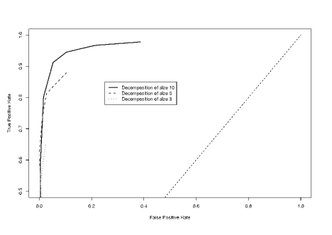
Figure 4: Comparison of decomposition sizes. Decomposition into cliques of maximal size 3, 5 and 10 using DGL:CV. The curves corresponds to models which arise by thresholding the final $\hat{\boldsymbol{\beta}}$-coefficient.

5.2 Performance for structure estimation

First, we compare DGL, DSF and DF. The performance for structure estimation is shown in ROC curves (see Fig. 5). For DSF the curve builds up by varying $s$ (compare section 4.1). Note, that the starting point of the curve of DSF coincides with DF. DGL starts from DGL:CV and uses hard-thresholding of $\hat{\boldsymbol{\beta}}$ for obtaining the values on the ROC curve. Note that during this hard-thresholding, the value of DGL:F is produced, too. We see that DSF and DGL lead to models which have approximately the same number of false positive and false negative edges, but the DGL is slightly favorable. The solution of DF has the largest false positive rate (as was expected since no model selection was done).

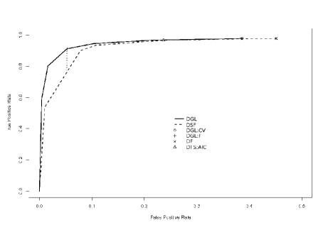
Figure 5: Comparison of decomposition approaches DGL, DSF and DF using $s_{max}=10$. The dotted vertical line corresponds to the difference in the true positive rate (number of correctly selected edges / number of true edges) for the two procedures when they are compared at the false positive rate (number of incorrectly selected edges / number of true gaps) of DGL:F. Note that the x-axis is shown only up to $0.5$.

Second, in Fig. 6 the alternative approaches WW and RF are compared with DGL. In order to keep a simple overview, the results for DSF are no longer shown. We see that our decomposition approach (DGL) slightly outperforms the alternative approaches WW and RF. Keep in mind that in addition to the advantage of our method in performance, RF does not yield an estimate for the parameter vector and WW does so only for binary variables, whereas our method is applicable to general multi-category variables.

Even though Fig. 5 and Fig. 6 only represent one simulated dataset, we observed a similar picture for other simulation settings. The lines for DGL and DSF are always very close, with DGL being slightly better and both methods being clearly superior to the global approaches. The reason why Fig. 5 and Fig. 6 only display results from one dataset is that the single final models cannot be averaged over different datasets as they have different positions on the curves for different datasets (different numbers of true and false positives). If we average over all these values, the result is not very meaningful anymore. However, we can average the differences of true positive rates for e.g. DGL and DSF where both methods have the same number of false positives as the solution of DGL:F (dotted vertical line in Fig. 5). The results of such comparisons are summarized in Table 2. We see that DGL yields a significantly (for significance level $\alpha=0.05$) higher true positive rate than the corresponding solutions of DSF and WW. On the other hand, the comparison between the solution of DGL and RF (at the false positive rate of DGL:F) shows no significant difference.

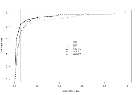
Figure 6: Comparison of DGL with WW and RF. For DGL the line builds up by thresholding the $\hat{\boldsymbol{\beta}}$-coefficient where $\lambda$ is chosen by cross-validation. For RF, the edges with least importance are successively eliminated and for WW, the tuning parameter $\lambda$ is varied. The grey vertical line indicates the false positive rate of DGL:F at which the true positive rates of the other methods are compared in Table 2.

Table 2: Comparison of true positive rates of different methods at the false positive rate of DGL:F (indicated in Fig. 5 and Fig. 6 by vertical lines).

	Mean difference	p-value (t-test)
tpr(DGL) - tpr(DSF)	0.052	0.036
tpr(DGL) - tpr(WW)	0.060	0.011
tpr(DGL) - tpr(RF)	0.013	0.256

5.3 Performance for estimation of cell probabilities

DGL, DSF, DF and WW yield estimates of the parameter vector $\boldsymbol{\beta}$ which can be immediately transformed into estimates of cell probabilities. In this section we will compare these methods with respect to the performance for estimating the cell probabilities. Recall that RF does not yield an estimate of the parameter vector and is therefore not included in this comparison.

All approaches considered in this section yield the parameter vector $\boldsymbol{\beta}$ only up to a constant. We need to ensure that the estimated cell probabilities add up to one. For sparse graphs, we can use the junction tree algorithm to calculate the normalising constant for the probabilities. For a detailed description see Lauritzen (1996).

We compare the estimated probabilities, using cross-validation for tuning parameters and using an expression which is up to a constant the Kullback-Leibler divergence between the estimated and the true probability (non-normalized Kullback-Leibler divergence):

$$-\log{\left(\prod_{i}\hat{p}_{i}^{p_{i}}\right)}=-\sum_{i}p_{i}\log{\hat{p}_{i}},$$ (11)

where $\mathbf{\hat{p}}$ is the estimated probability vector and $\mathbf{p}$ denotes the true probability vector. As this sum requires the calculation of $2^{40}\approx 10^{12}$ components of $\mathbf{\hat{p}}$ and $\mathbf{p}$ and the summation of the two huge vectors, this is computationally not feasible. To avoid this problem, we calculate an empirical version by simulating one million observations from the graph in Fig. 3 and summing over these $10^{6}$ values only.

Figure 7: Mean empirical (non-normalized) Kullback-Leibler distance between true and estimated probability in dependence of the percentage of thresholded coefficients. The vertical line indicates the average of percentages of thresholded coefficients using the thresholding rule from section 3.3.

The results are summarized in Table 3. We see that DGL:F, DSF:AIC and DF perform similarly and WW:MIN is clearly inferior. For WW:CV, which is indicated in Fig. 6, the normalizing constant could not be computed. This is because the CV-optimal solution almost corresponds to the full model and thus, the junction tree algorithm is not feasible. The maximal computable solutions of WW still correspond to very large models, which on average involve $22.05\%$ of all possible edges, compared to $17.01\%$ for DGL:F and $11.66\%$ for the true graph.

Table 4 provides further insight about significance of the differences in Table 3. All methods are compared against each other using a paired t-test for the empirical (non-normalized) Kullback-Leibler divergences and the $p$-values are reported. One can see that there is no significant (at significance level $\alpha=0.05$) difference for the decomposition approaches, whereas they are all superior to WW. This provides evidence that the decomposition of the model is more crucial than the effective choice of the log-linear model fitting procedure afterwards.

Furthermore, it is worthwhile stating that the thresholding of the coefficients (see section 3.3) does hardly influence the likelihood as can be seen in Fig. 7. On average, $35\%$ of the coefficients are thresholded as indicated by the dotted line. However, for these threshold-optimal solutions, calculated as described in section 3.3, the empirical (non-normalized) Kullback-Leibler divergence is approximately the same as for the non-thresholded model.

Table 3: Mean empirical (non-normalized) Kullback-Leibler divergence between true and estimated probabilities. The $p$-values for all the pairwise comparisons are given in Table 4.

	Mean	SD
DGL:F	4.0080	0.0204
DSF:AIC	4.0242	0.0217
DF	4.0223	0.0099
WW:MIN	4.3360	0.1094

Table 4: All possible pairwise comparisons between models: $p$-values of a paired t-test for the equality of (non-normalized) Kullback-Leibler divergence.

	DSF:AIC	DF	WW:MIN
DGL:F	0.1030	0.0677	4.7 $10^{-6}$
DSF:AIC	-	0.8080	6.0 $10^{-6}$
DF	-	-	7.5 $10^{-6}$

6 Application to Tissue Microarray Data

6.1 Tissue Microarray technology

The central motivation that led to this work was to fit a graphical model to discrete expression levels of biomarkers resulting from Tissue Microarray (TMA) experiments. Tissue Microarray technology allows rapid visualization of molecular targets in thousands of tissues at a time, either at DNA, RNA or protein level. Tissue Microarrays are composed of hundreds of tissue sections from different patients arrayed on a single glass slide. With the use of immunohistochemical staining, they provide a high-throughput method to analyze potential biomarkers on large patient samples. The assessment of the expression level of a biomarker is usually performed by the pathologist on a categorical scale: expressed/not expressed, or the level of expression.

Tissue Microarrays are powerful for validation and extension of findings obtained from genomic surveys such as cDNA microarrays. cDNA microarrays are useful to analyze a huge number of genes, e.g. a couple of thousands in one specimen at a time. In contrast, TMAs are applicable to the analysis of one target at a time, denoted as biomarker, but in up to 1000 tissues on each slide.

The analysis of the interaction pattern of these biomarkers and in particular the estimation of the graphical model associated with the underlying discrete random variables are of bio-medical importance. These graph-based patterns can deliver valuable insight into the underlying biology. A detailed description of the Tissue Microarray technology can be found in Kallioniemi et al. (2001).

6.2 Estimation of graphical model

Our TMA dataset consists of Tissue Microarray measurements from renal cell carcinoma patients. We have information from 1116 patients, 831 thereof having a clear cell carcinoma tumor, which is the tumor of interest here. We have identified 18 biomarkers from which we have information for the majority of the patients. Among 831 ccRCC (clear cell renal cell carcinoma) observations, 527 observations are complete with all biomarker measurements available. For 87 observations one measurement was missing, 64 and 30 observations had 2 or 3 missing values, respectively. 123 observations contained more than 3 missing values and were ignored in the analysis. For the observations with 1, 2 or 3 missing values, multiple imputation was applied using the R package mice (Van Buuren and Oudshoorn, 2007). From 18 biomarkers, 9 are binary and 9 have 3 levels.

Using DGL:F, we estimated a graphical model to the TMA data. The resulting graph is displayed in Fig. 8. The thickness of the line corresponds to the $\ell_{2}$-norm of the respective interaction coefficients. Two biomarkers connected by a thick line, as is the case for nuclear p27 and cytoplasmic p27, indicates a strong interaction. The kinase inhibitor p27 exhibits its function in the cell nucleus and therefore recent studies have focused on nuclear p27 expression. Our graphical log-linear model however shows a tight association between nuclear and cytoplasmic expression of p27. Therefore it can be speculated that both nuclear and cytoplasmic presence is required to ensure proper function of p27. It has been shown that in renal tumors, the von Hippel-Lindau protein (VHL protein) is upregulating the expression of the tumor suppressor p27 (Osipov et al., 2002). The graphical model here provides supporting evidence that VHL indeed regulates p27, and the corresponding $\boldsymbol{\beta}$ coefficient (not displayed here) implies that it is a positive regulation.

Furthermore it has been shown in vitro by Roe et al. (2006) that VHL increases p53 expression which is a tumor suppressor. In our model it seems as if p53 is conditionally independent of VHL. Indeed, it has long been known that p53 activates expression of p21 (e.g. Kim (1997)). This dependence is displayed very clearly in the graphical model. We can therefore view the p53-p21 pathway with its strong interaction as one unit and it is therefore very reasonable that nuclear VHL interacts with p53. As nuclear VHL is only expressed in 14% of the tumors, and it further makes sense from a biological point of view that the strong interaction between VHL and the p21-p53 pathway is in fact a causal relation, we can indeed speculate that the loss of VHL deactivates the tumor suppressor p53 which in turn favors tumor development.

CA9, Glut1 and Cyclin D1 are all hypoxia-inducible transcription factor (HIF) target genes (Wenger et al., 2005). HIF has not been measured but we can clearly see that all these HIF targets are connected by a rather thick line implying that they might react to a common gene. In addition, CD10 strongly interacts with Glut1 a known HIF target which suggests that CD10 might also be regulated by HIF. The reduction of E-Cadherin expression has been found to be negatively correlated with HIF expression in Imai et al. (2003). This is supported by a strong negative interaction between E-Cadherin and CA9 which is positively correlated with HIF expression (not measured).

A lot of supporting evidence has been delivered for already existing theories. However, two strong interactions, one between PAX2 and nuclear p21 and the other between PAX2 and Cyclin D1 cannot be immediately explained. PAX2 is absent in normal renal tubular epithelial cells but expressed in many clear cell renal cell carcinoma tumours (see Mazal et al. (2005)). Its frequent expression together with the strong interaction with the p21-p53 pathway, Cyclin D1 and PTEN make PAX2 an interesting and possibly important molecular parameter whose exact function and role still remains to be elucidated.

A more detailed discussion of bio-medical implications is given in Dahinden et al. (2009).

Figure 8: Estimated graphical model from Tissue Microarray data

7 Discussion

We have proposed a decomposition approach to estimating log-linear models for large contingency tables and for fitting discrete graphical models. In a simulation study we have compared various algorithms and concluded that our procedures are very competitive. It seems that the decomposition of the problem is much more crucial than the choice of the algorithm to handle the smaller decomposed datasets: no matter whether DGL, DSF or DF is applied, the resulting models are superior to non-decomposition approaches such as WW and RF for model selection as well as for probability or parameter estimation.

Maybe most important is the computational feasibility of our procedure for large contingency tables. The proposed method is scalable to orders of realistic complexity (e.g. dozens up to hundreds of factors) where most or all other existing algorithms become infeasible. In particular, our procedure is not only capable of handling binary data but can easily deal with factors with more levels. Furthermore, with DGL one doesn’t risk the nonexistence of the parameter estimator in case of sampling zeroes in the contingency table as this might arise when using the MLE. Our procedure not only fits a graphical model but also yields an estimation of the parameter vector $\boldsymbol{\beta}$ in a log-linear model and therefore of the cell probabilities. All this is achieved with good performance in comparison to other methods. As a drawback, if the true underlying graph has a clique which is larger than our decomposition size, then some of the edges in the graph are necessarily lost.

We apply the proposed approach to a problem in molecular biology and we find supporting evidence for dependencies between biomarkers which have already been found to exist in vitro or some even in renal tumors, the domain of our application. However, some strong interactions cannot be explained immediately and therefore, new biological hypotheses arise.

The R package LLdecomp for computing a decomposition as described in this paper (i.e., recursively finding cliques and separators) is available at http://www.r-project.org.

We would like to thank an Associate Editor and two referees for their constructive comments. We would also like to thank Dr. Peter Schraml for valuable comments, suggestions and discussions regarding biological interpretation.

Conflict of Interest Statement
The authors have declared no conflict of interest.

References

- Bishop et al. (1975) Bishop, Y., Fienberg, S. and Holland, P. (1975) Discrete Multivariate Analysis. MIT Press, Cambridge, Massachusetts and London, UK.
- Breiman (2001) Breiman, L. (2001) Random forests. Machine Learning, 45, 5–32.
- Christensen (1991) Christensen, R. (1991) Linear Models for Multivariate Time Series, and Spatial Data. Springer-Verlag.
- Dahinden et al. (2009) Dahinden, C., Ingold, B., Wild, P., Boysen, G., Luu, V.-D., Montani, M., Kristiansen, G., Bühlmann, P., Moch, H. and Schraml, P. (2009) Mining tissue microarray data to unhide dysregulated tumor suppressor pathways in clear cell renal cell cancer: loss of p27 and pten is critical for tumor progression. To appear in Clinical Cancer Research.
- Dahinden et al. (2007) Dahinden, C., Parmigiani, G., Emerick, M. and Bühlmann, P. (2007) Penalized likelihood for sparse contingency tables with an application to full-length cDNA libraries. BMC Bioinformatics, 8, 476.
- Darroch et al. (1980) Darroch, J., Lauritzen, S. and Speed, T. (1980) Markov fields and log-lineaer interaction models for contingency tables. Ann. Statist., 8, 522–539.
- Imai et al. (2003) Imai, T., Horiuchi, A., Wang, C., Oka, K., Ohira, S., Nikaido, T. and Konishi, I. (2003) Hypoxia Attenuates the Expression of E-Cadherin via Up-Regulation of SNAIL in Ovarian Carcinoma Cells. The American Journal of Pathology, 163, 1437–1447.
- Jackson et al. (2007) Jackson, L., Gray, A. and Fienberg, S. (2007) Sequential category aggregation and partitioning approach for multy-way contingency tables based on survey and census data. Preprint.
- Kallioniemi et al. (2001) Kallioniemi, O., Wagner, U., Kononen, J. and Sauter, G. (2001) Tissue microarray technology for high-throughput molecular profiling of cancer. Hum. Mol. Genet., 10, 657–662.
- Kim (2005) Kim, S. (2005) Log-linear modelling for contingency tables by using marginal model structures. Research Report 05, Division of Applied Mathematics, Korea Advanced Institute of Science and Technology.
- Kim (1997) Kim, T. (1997) In vitrotranscriptional activation of p21 promoter by p53. Biochemical and Biophysical Research Communication, 234, 300–302.
- Lauritzen (1996) Lauritzen, S. (1996) Graphical Models. Oxford Statistical Science Series, 17. Oxford Clarendon Press.
- Mazal et al. (2005) Mazal, P., Stichenwirth, M., Koller, A., Blach, S., Haitel, A. and Susani, M. (2005) Expression of aquaporins and pax-2 compared to cd10 and cytokeratin 7 in renal neoplasms: a tissue microarray study. Modern Pathology, 18, 535–40.
- Olesen and Madsen (2002) Olesen, K. and Madsen, A. L. (2002) Maximal prime subgraph decomposition of Bayesian networks. IEEE Transactions on Systems, Man, and Cybernetics, Part B, 32.
- Osipov et al. (2002) Osipov, V., Keating, J. T., Faul, P. N., Loda, M. and Dattas, M. W. (2002) Expression of p27 and VHL in renal tumors. Applied Immunohistochemistry & Molecular Morphology, 10, 344–350.
- Ravikumar et al. (2009) Ravikumar, P., Wainwright, M. and Lafferty, J. (2009) High-dimensional graphical model selection using -regularized logistic regression. To appear in Annals of Statistics.
- Roe et al. (2006) Roe, J., Kim, H., Lee, S., Kim, S., Cho, E. and Youn, H. (2006) p53 stabilization and transactivation by a von hippel-lindau protein. Molecular Cell, 22, 395–405.
- Strobl et al. (2007) Strobl, C., Boulesteix, A., Zeileis, A. and Hothorn, T. (2007) Bias in random forest variable importance measures: Illustrations, sources and a solution. BMC Bioinformatics, 8, 25.
- Tibshirani (1996) Tibshirani, R. (1996) Regression shrinkage and selection via the lasso. J. Royal Statist. Soc., 58, 267–288.
- Van Buuren and Oudshoorn (2007) Van Buuren, S. and Oudshoorn, C. (2007) mice: Multivariate Imputation by Chained Equations. URL http://web.inter.nl.net/users/S.van.Buuren/mi/hmtl/mice.htm. R package version 1.16.
- Wainwright et al. (2007) Wainwright, M., Ravikumar, P. and Lafferty, J. (2007) High-dimensional graphical model selection using -regularized logistic regression. In Advances in Neural Information Processing Systems 19 (eds. B. Schölkopf, J. Platt and T. Hoffman), 1465–1472. Cambridge, MA: MIT Press.
- Wenger et al. (2005) Wenger, R., Stiehl, D. and Camenisch, G. (2005) Integration of oxygen signaling at the consensus hre. Science Signaling: Signal Transduction Knowledge Environment (STKE), 2005, re12.
- Yuan and Lin (2006) Yuan, M. and Lin, Y. (2006) Model selection and estimation in regression with grouped variables. Journal of the Royal Statistical Society, 68, 49–67.