Proton Polarimeter Calibration between 82 and 217 MeV
Abstract
The proton analyzing power in carbon has been measured for energies of 82 to 217 MeV and proton scattering angles of 5 to 41∘. The measurements were carried out using polarized protons from the elastic scattering 1H reaction and the Focal Plane Polarimeter (FPP) in Hall A of Jefferson Lab. A new parameterization of the FPP p-C analyzing power was fit to the data, which is in good agreement with previous parameterizations and provides an extension to lower energies and larger angles. The main conclusions are that all polarimeters to date give consistent measurements of the carbon analyzing power, independently of the details of their construction and that measuring on a larger angular range significantly improves the polarimeter figure of merit at low energies.
keywords:
analyzing power , polarization , polarimeterPACS:
41.85.Qg , 95.75.Hi1 Introduction
In order to extract polarizations from asymmetries in proton-carbon scattering, accurate values of the analyzing power, , are needed. The analyzing power depends on the strength of the spin-orbit coupling and is a function of the proton kinetic energy, , and of the polar scattering angle, . We have used a functional form similar to those used previously [1, 2], to obtain a new parameterization in the energy range of 82 to 217 MeV and proton scattering angles in carbon between 5 and 41∘. The new parameterization is in good agreement with previous parameterizations [2, 3, 4, 5] and provides an extension to lower energies and larger scattering angles. To date, the new parameterization has been used in three low energy polarization experiments [6, 7, 8].
2 Method
The experiment was carried out in Hall A of Jefferson Lab [9]. The primary elastic scattering 1H reaction provided the source of polarized protons for the calibration. The scattered proton polarization was determined independently of our knowledge of .
A continuous, polarized electron beam with polarization ranging from 80 to 85% was produced using a strained gallium-arsenide (GaAs) source [10, 11]. The polarization in Hall A was limited to = 38–41% due to multi-hall running. The beam helicity was flipped pseudo-randomly at 30 Hz, with negligible beam charge asymmetry between the two helicity states. The electron beam was accelerated to either 362 or 687 MeV and then scattered from a 15 cm long liquid hydrogen target.
The scattered protons were detected in the left High Resolution Spectrometer (HRS) [12], made up of one dipole and three quadrupole magnets. Vertical drift chambers were used to track the protons after deviation by the magnetic field of the dipole, allowing a determination of the momentum with a resolution of 2 10-4 [13]. The proton target quantities (transverse position), (, where is the displacement in dispersive plane and is along the spectrometer axis), () and (fractional deviation of momentum from central trajectory) were reconstructed from the proton trajectory using the HRS optics matrix. Triggering was performed using a coincidence between two scintillator planes, S1 and S2, each made up of six panels. The scintillators S1 and S2 are both located before the Focal Plane Polarimeter (FPP) carbon analyzer.
The FPP, downstream of the VDCs and trigger panels, measured the recoil polarization of the protons through a secondary scattering of the protons from a carbon block “analyzer”. Spin-orbit coupling between the proton spin and angular momentum about the analyzer carbon nucleus leads to an asymmetry in the azimuthal scattering angle, , reconstructed from the front and rear proton tracks. A detailed description of the polarimeter can be found in [14, 15]. The FPP measures the inclusive C() reaction at the low energies reported here, but also the inclusive C(), where is a charged particle, for energies above pion production threshold.
Cuts were made on the reconstructed proton target quantities of 65 mm, 65 mrad, 38 mrad and 0.045, in order to ensure that the protons originated in the target volume and traversed the HRS in a phase space region with high detection efficiency. To remove the majority of multiple scattering events due to Coulomb interactions between the proton and carbon nuclei, a cut on the FPP polar angle of 5∘ was made. A conetest cut was used to remove instrumental asymmetries [16]. In order to ensure that all FPP scattering events originated from within the carbon block, a cut was made around the location (along the spectrometer axis) of closest approach between the front and rear FPP tracks. A cut of 1 cm or less was also placed on the distance of closest approach between the front and rear tracks.
Three carbon block thicknesses were used: 0.75, 2.25 and 3.75”. The carbon thickness was varied according to GEANT [17] Monte Carlo studies in order to maximize the figure of merit (), which is a measure of how many events contribute to the scattering asymmetry and is given by the following integral over or approximate summation over bins in :
| (1) |
where is the analyzing power and is the FPP efficiency, given by the fraction of events passing the target cuts and having tracks in the front FPP chambers which pass the FPP cuts. For the purposes of choosing carbon thicknesses, the Monte Carlo studies assumed to follow the earlier parameterization of [2]. A summary of the primary 1H reaction kinematics and FPP parameters can be found in Table 1.
3 Analysis
The recoil transferred polarization was determined by a maximum likelihood method using the difference of the azimuthal distributions at the focal plane corresponding to the two beam helicity states. After spin transport through the spectrometer using COSY [18], a differential algebra based code, the transferred polarization products at the target, and , were obtained. The ratio of these products was used to calculate the proton elastic form factor ratio, , with the following equation [14]:
| (2) |
where and are the energies of the incident and scattered electron, respectively, is the electron scattering angle in the laboratory frame and is the proton mass. Note that knowledge of the analyzing power and beam polarization are not required as they cancel. The form factor ratio calculated with Equation 2 was in turn used in the following derivations for the transferred polarization components at the target [19, 20, 21, 22]:
| (3) |
| (4) |
where , is the four-momentum transfer squared and is the longitudinal polarization of the virtual photon. and calculated with equations 3 and 4, respectively, were combined with the transferred polarization products at the target obtained through azimuthal asymmetries, and , to extract the analyzing power and the statistical uncertainty [14], where was taken to be the average beam helicity associated with the data.
The extracted analyzing power data can be found in Tables 2 and 3 for incident electron beam energies of 362 and 687 MeV, respectively. The total systematic uncertainty due to uncertainties in beam polarization, spin transport, reconstruction of FPP scattering angles, proton momentum and beam energy is also shown. Table 4 presents the weighted average analyzing power, FPP efficiency and figure of merit, calculated using the summation approximation of equation 1 and the data in Tables 2 and 3.
The functional form used to fit the extracted analyzing power is similar to the “low energy fit” used by McNaughton et al. [1, 2]. It is given by:
| (5) |
where and is the proton momentum in GeV/c at the center of the carbon analyzer. Note that the functional form given satisfies the physical constraint that the analyzing power vanish at = 0 and 180∘. The coefficients , , and are polynomials of the momentum. The last parameter, , was added in order to improve the quality of fit. The coefficients are expanded as follows:
| (6) |
where are the parameters of the fit. In order to obtain a numerically stable fit, the parameter was set to the middle of the momentum range at the center of the carbon block, or 0.55 GeV/c. The quality of the obtained fits was largely insensitive to the choice of , provided it was roughly in the middle of the momentum range being fit. The energy loss was approximated by dividing the carbon block into 1 cm layers and calculating the energy loss at each layer using a parameterization of the proton stopping power in carbon [23]. The procedure was repeated up to the center of the carbon block resulting in an average total energy loss. The entire data set found in Tables 2 and 3 was fit simultaneously and the parameters of this fit can be found in Table 5.
To determine the statistical uncertainty of the fit the data points were shifted randomly within their statistical error bars and the resulting distribution was refit. The procedure was repeated 100 times and the maximum shift from central analyzing power value at each value of and was taken as the statistical uncertainty of the fit at that point. The systematic uncertainty of the fit was determined by fitting the distributions shifted both upward and downward by the systematic uncertainty of the data and the half width at each value of and was taken as the systematic uncertainty of the fit at that point. The statistical and systematic contributions to the total fit uncertainty at each point were then added in quadrature. The fit uncertainty was then parameterized as a function of and using the functional form of equation 5 and the parameters of the error fit can be found in Table 6. The uncertainty of the parameterized analyzing power can therefore be calculated for any kinetic energy at carbon center between 82 and 217 MeV and scattering angle between 5 and 41∘.
4 Results
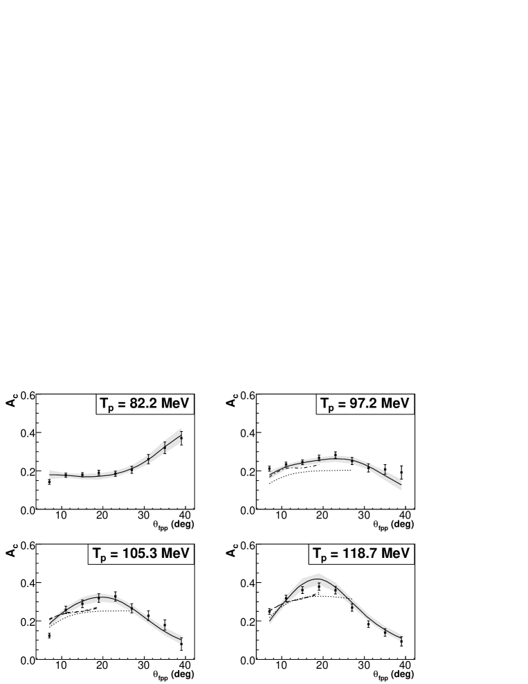
Figures 1 and 2 compare the new (solid), the “low energy” McNaughton [2] (dashed), the “low energy” Aprile-Giboni [3] (dashed dotted), the Waters [4] (dotted) and the Pospischil [5] (dashed double dotted) parameterizations to the new low energy data. Note that low energy data was also taken by M. Ieiri et al. [24] for kinetic energies at carbon center between 20 and 84 MeV and scattering angles between 15 and 80∘ and by S.M. Bowyer et al. [25] for kinetic energies at carbon center between 120 and 200 MeV and scattering angles between 6 and 23∘. The fit uncertainty of the new parameterization, as described above, is denoted by the gray band. The “low energy” Aprile-Giboni parameterization was done for scattering angles of 5–20∘, energies at carbon center of 90–386 MeV and a carbon block thickness of 3 cm. The Waters parameterization was done for scattering angles of 3.5–28∘, energies at carbon center of 90–450 MeV and carbon block thicknesses of 3 and 6 cm. Note that Waters et al. quote a 10–20% uncertainty on their fit for energies between 90 and 100 MeV. The “low energy” McNaughton parameterization was fit to the world database at that time, including data from Aprile-Giboni et al. [3] and Waters et al. [4], with carbon thicknesses ranging from 3 to 12.7 cm. It is valid for scattering angles between 5 and 20∘ and kinetic energies at the center of the carbon between 100 and 450 MeV. The parameterization of Pospischil et al., with a carbon block thickness of 7 cm, used a larger angular range of 15.7–43.1∘ but a narrow energy range of 160–200 MeV. It is shown only in the = 171.1 MeV panel of Figure 2.
There is a good agreement between the new parameterization and the older ones in the energy/angle regimes for which they were intended, considering all fits were done for different polarimeters and for varying carbon block thicknesses. Consistency between different polarimeters has been observed before and is generally expected. This is in part because the energy range covered by most polarimeters in a single measurement is sufficiently small that the variation of analyzing power with energy is essentially linear. The new parameterization provides an extension down to an energy of 82 MeV and up to a scattering angle of 41∘.
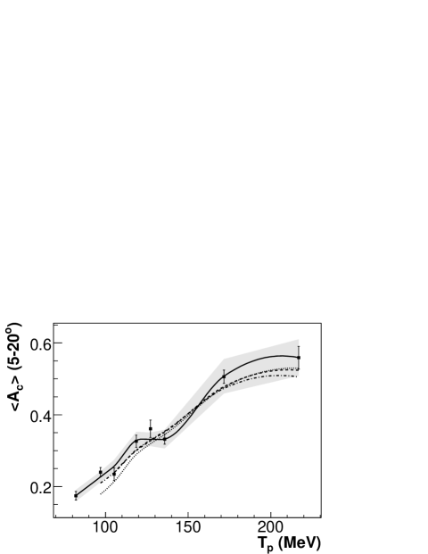
The energy dependence of the weighted average analyzing power is shown for the angular range of in Figure 3, which again shows a very good agreement between the new data and the parameterizations in the energy/angle regimes for which the previous parameterizations were intended.
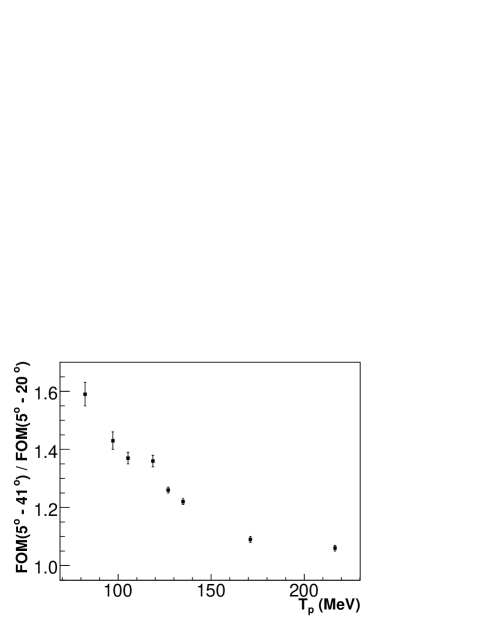
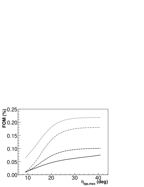
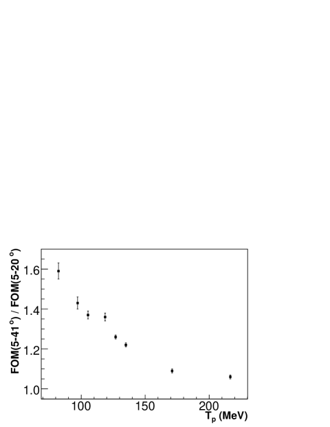
A higher figure of merit results in more useful events and a lower statistical uncertainty on extracted polarization observables. The figure of merit as a function of maximum scattering angle is shown in Figures 4 and 5 for beam energies 362 and 687 MeV, respectively. For the highest energies, the dependence of the figure of merit on maximum scattering angle is relatively flat beyond 25∘. For the lowest energies, the figure of merit increases steadily as the maximum scattering angle is increased to 41∘. By extending the maximum scattering angle of the parameterization, one obtains an improvement of up to 1.6 times in the figure of merit at low energies, as can be seen in Figure 6.
5 Conclusion
A new parameterization, similar to that of [2], was determined for p-C analyzing power in the 82 to 217 MeV energy region, and found to be in good agreement with the previous parameterizations in the energy and angular regimes for which they were intended. This corroborates that the various polarimeters built to date are measuring a property of inclusive proton-carbon scattering insensitive to details of how the polarimeters are constructed. The extension made for energies between 82 and 90 MeV and for scattering angles between 20 and 41∘ increased the figure of merit by a factor of 1.6 at low energies. Any new polarimeters for low energy protons should take advantage of the increase in figure of merit from large-angle scattering in the polarimeter.
Acknowledgments
We thank the Jefferson Lab physics and accelerator divisions for their contributions. This work was supported by the U.S. Department of Energy, the U.S. National Science Foundation, Argonne National Laboratory under contract DE-AC02-06CH11357, the Israel Science Foundation, the Korea Science Foundation, the US-Israeli Bi-National Scientific Foundation, the Natural Sciences and Engineering Research Council of Canada, the Killam Trusts Fund and the Walter C. Sumner Foundation. Jefferson Science Associates operates the Thomas Jefferson National Accelerator Facility under DOE contract DE-AC05-06OR23177. The polarimeter was funded by the U.S. National Science Foundation, grants PHY 9213864 and PHY 9213869.
| Analyzer | ||||
| (MeV) | (deg) | (MeV/c) | (MeV) | Thickness |
| (inches) | ||||
| 362 | 28.3 | 476.1 | 82.2 | 0.75 |
| 362 | 23.9 | 503.2 | 97.2 | 0.75 |
| 362 | 18.8 | 526.3 | 105.3 | 0.75 |
| 362 | 18.8 | 526.3 | 105.3 | 2.25 |
| 362 | 14.0 | 541.4 | 118.7 | 0.75 |
| 687 | 47.0 | 583.9 | 126.9 | 2.25 |
| 687 | 44.2 | 621.1 | 134.9 | 3.75 |
| 687 | 40.0 | 674.0 | 171.1 | 3.75 |
| 687 | 34.4 | 740.3 | 216.6 | 3.75 |
| stat syst | |||
|---|---|---|---|
| (MeV) | (deg) | (%) | |
| 82.2 | 7 | 0.143 0.010 0.007 | 0.33 |
| 11 | 0.177 0.008 0.008 | 0.42 | |
| 15 | 0.180 0.008 0.008 | 0.45 | |
| 19 | 0.190 0.009 0.009 | 0.35 | |
| 23 | 0.186 0.011 0.008 | 0.22 | |
| 27 | 0.206 0.015 0.010 | 0.12 | |
| 31 | 0.261 0.020 0.013 | 0.07 | |
| 35 | 0.320 0.026 0.016 | 0.04 | |
| 39 | 0.371 0.031 0.017 | 0.03 | |
| 97.2 | 7 | 0.212 0.010 0.009 | 0.28 |
| 11 | 0.234 0.007 0.010 | 0.41 | |
| 15 | 0.245 0.007 0.010 | 0.41 | |
| 19 | 0.268 0.009 0.012 | 0.29 | |
| 23 | 0.283 0.011 0.012 | 0.17 | |
| 27 | 0.252 0.015 0.011 | 0.10 | |
| 31 | 0.216 0.019 0.011 | 0.06 | |
| 35 | 0.208 0.023 0.009 | 0.04 | |
| 39 | 0.192 0.033 0.010 | 0.03 | |
| 105.3 | 7 | 0.124 0.008 0.009 | 1.93 |
| 11 | 0.258 0.009 0.017 | 0.68 | |
| 15 | 0.290 0.009 0.018 | 0.58 | |
| 19 | 0.319 0.011 0.020 | 0.37 | |
| 23 | 0.328 0.014 0.020 | 0.20 | |
| 27 | 0.266 0.017 0.017 | 0.11 | |
| 31 | 0.228 0.021 0.014 | 0.06 | |
| 35 | 0.179 0.024 0.010 | 0.04 | |
| 39 | 0.080 0.032 0.007 | 0.03 | |
| 118.7 | 7 | 0.249 0.008 0.012 | 0.26 |
| 11 | 0.318 0.007 0.014 | 0.39 | |
| 15 | 0.361 0.007 0.016 | 0.36 | |
| 19 | 0.379 0.009 0.017 | 0.25 | |
| 23 | 0.360 0.011 0.016 | 0.16 | |
| 27 | 0.270 0.013 0.014 | 0.11 | |
| 31 | 0.184 0.015 0.008 | 0.09 | |
| 35 | 0.140 0.017 0.009 | 0.06 | |
| 39 | 0.094 0.023 0.008 | 0.03 |
| stat syst | |||
|---|---|---|---|
| (MeV) | (deg) | (%) | |
| 126.9 | 7 | 0.244 0.006 0.016 | 1.34 |
| 11 | 0.379 0.007 0.024 | 1.24 | |
| 15 | 0.433 0.008 0.027 | 0.97 | |
| 19 | 0.453 0.010 0.029 | 0.59 | |
| 23 | 0.415 0.012 0.026 | 0.34 | |
| 27 | 0.339 0.016 0.022 | 0.21 | |
| 31 | 0.270 0.018 0.017 | 0.15 | |
| 35 | 0.198 0.023 0.013 | 0.10 | |
| 39 | 0.120 0.029 0.008 | 0.07 | |
| 134.9 | 7 | 0.179 0.004 0.008 | 2.35 |
| 11 | 0.403 0.005 0.016 | 1.47 | |
| 15 | 0.443 0.005 0.017 | 1.14 | |
| 19 | 0.480 0.007 0.019 | 0.68 | |
| 23 | 0.436 0.009 0.018 | 0.38 | |
| 27 | 0.353 0.011 0.014 | 0.21 | |
| 31 | 0.295 0.016 0.011 | 0.13 | |
| 35 | 0.236 0.024 0.009 | 0.08 | |
| 39 | 0.181 0.022 0.007 | 0.05 | |
| 171.1 | 7 | 0.394 0.006 0.013 | 1.38 |
| 11 | 0.559 0.006 0.019 | 1.28 | |
| 15 | 0.600 0.007 0.020 | 0.93 | |
| 19 | 0.493 0.009 0.018 | 0.60 | |
| 23 | 0.334 0.010 0.013 | 0.44 | |
| 27 | 0.203 0.011 0.007 | 0.33 | |
| 31 | 0.109 0.012 0.004 | 0.25 | |
| 35 | 0.048 0.014 0.002 | 0.18 | |
| 39 | -0.043 0.036 0.004 | 0.11 | |
| 216.6 | 7 | 0.537 0.006 0.030 | 1.23 |
| 11 | 0.677 0.006 0.037 | 1.15 | |
| 15 | 0.584 0.007 0.033 | 0.85 | |
| 19 | 0.380 0.008 0.022 | 0.67 | |
| 23 | 0.219 0.008 0.012 | 0.59 | |
| 27 | 0.134 0.008 0.008 | 0.53 | |
| 31 | 0.047 0.009 0.003 | 0.41 | |
| 35 | 0.045 0.048 0.017 | 0.30 | |
| 39 | -0.060 0.021 0.003 | 0.18 |
| (MeV) | (%) | (%) | |
|---|---|---|---|
| 82.2 | 2.03 | 0.186 0.010 0.009 | 0.07 |
| 97.2 | 1.80 | 0.243 0.010 0.010 | 0.11 |
| 105.3 | 4.01 | 0.239 0.011 0.015 | 0.20 |
| 118.7 | 1.72 | 0.307 0.009 0.014 | 0.17 |
| 126.9 | 5.02 | 0.354 0.009 0.023 | 0.66 |
| 134.9 | 6.50 | 0.336 0.006 0.014 | 0.81 |
| 171.1 | 5.49 | 0.423 0.009 0.015 | 1.16 |
| 216.6 | 5.91 | 0.391 0.010 0.023 | 1.31 |
| Coefficient | Value | Unit |
|---|---|---|
| p0 | 0.55 | (GeV/c) |
| a0 | 4.0441 | (GeV/c)-1 |
| a1 | 19.313 | (GeV/c)-2 |
| a2 | 119.27 | (GeV/c)-3 |
| a3 | 439.75 | (GeV/c)-4 |
| a4 | 9644.7 | (GeV/c)-5 |
| b0 | 6.4212 | (GeV/c)-2 |
| b1 | 111.99 | (GeV/c)-3 |
| b2 | -5847.9 | (GeV/c)-4 |
| b3 | -21750 | (GeV/c)-5 |
| b4 | 973130 | (GeV/c)-6 |
| c0 | 42.741 | (GeV/c)-4 |
| c1 | -8639.4 | (GeV/c)-5 |
| c2 | 87129 | (GeV/c)-6 |
| c3 | 8.1359 | (GeV/c)-7 |
| c4 | -2.1720 | (GeV/c)-8 |
| d0 | 5826.0 | (GeV/c)-6 |
| d1 | 2.4701 | (GeV/c)-7 |
| d2 | 3.3768 | (GeV/c)-8 |
| d3 | -1.1201 | (GeV/c)-9 |
| d4 | -1.9356 | (GeV/c)-10 |
| Error | Value | Unit |
|---|---|---|
| Coefficient | ||
| p | 0.55 | (GeV/c) |
| a | 0.34687 | (GeV/c)-1 |
| a | 3.8266 | (GeV/c)-2 |
| a | 11.635 | (GeV/c)-3 |
| a | -314.18 | (GeV/c)-4 |
| a | 1015.1 | (GeV/c)-5 |
| b | 0.21579 | (GeV/c)-2 |
| b | 288.29 | (GeV/c)-3 |
| b | -13736. | (GeV/c)-4 |
| b | -1.5821 | (GeV/c)-5 |
| b | 2.2523 | (GeV/c)-6 |
| c | 938.40 | (GeV/c)-4 |
| c | -4961.8 | (GeV/c)-5 |
| c | 4.0190 | (GeV/c)-6 |
| c | 3.3034 | (GeV/c)-7 |
| c | -5.8401 | (GeV/c)-8 |
| d | -4910.9 | (GeV/c)-6 |
| d | 1.5133 | (GeV/c)-7 |
| d | -1.3127 | (GeV/c)-8 |
| d | -2.7446 | (GeV/c)-9 |
| d | 2.8556 | (GeV/c)-10 |

References
- [1] Ransome, R.D. et al., Nucl. Instr. and Meth. 201 (1982) 315 and references within.
- [2] McNaughton, M.W. et al., Nucl. Instr. and Meth. A 241 (1985) 435.
- [3] Aprile-Giboni, E. et al., Nucl. Instr. and Meth. 215 (1983) 147;
-
[4]
Waters, G. et al., Nucl. Instr. and Meth. 153 (1978) 401;
Hausser, O. et al., Nucl Instr. and Meth. A 254 (1987) 67. - [5] Pospischil, Th. et al., Nucl. Instr. and Meth. A 483 (2002) 713.
- [6] Ron, G. et al., Phys. Rev. Lett. 99 (2007) 202002.
- [7] JLab experiment E08-007, J. Arrington, D. Day, R. Gilman, G. Ron, D. Higinbotham, A.J. Sarty, spokespersons.
- [8] Glister, J. et al., Polarization Observables below 360 MeV in Deuteron Photodisintegration, Phys. Rev. Lett., to be submitted.
- [9] Leemann, C.W., Douglas, D.R., Krafft, G.A., Ann. Rev. Nucl. Part. Sci. 51 (2001) 413.
- [10] Sinclair, C.K., Adderley, P.A., Dunham, B.M., Hansknecht, J.C., Hartmann, P., Poelker, M., Price, J.S., Rutt, P.M., Schneider, W.J., Steigerwald, M., Phys. Rev. ST Accel. Beams 10 (2007) 023501.
- [11] Hernandez-Garcia, C., Stutzman, M.L., O’Shea, P.G., Phys. Today 61N2 (2008) 44.
- [12] Alcorn, J. et al., Nucl. Instr. and Meth. A 522 (2004) 294.
- [13] Fissum, K.G. et al., Nucl. Instr. and Meth. A 474 (2001) 108.
-
[14]
Punjabi, V. et al., Phys. Rev. C 71 (2005) 055202;
Publisher s Note, Phys. Rev. C 71 (2005) 069902. - [15] Jones, M.K. et al., in AIP Conference Proceedings No. 412, edited by T.W. Donnelly (AIP, New York, 1997), p. 342.
- [16] Roche, R., Ph.D. Thesis, Florida State University, 2003.
- [17] Agostinelli, S. et al., Nucl. Instr. and Meth. A 506 (2003) 250.
- [18] Berz, M., Hoffmann, H.C., Wollnik, H., Nucl. Instr. and Meth. A 258 (1987) 402.
- [19] Akhiezer, A.I. and Rekalo, M.P., Sov. Phys. Dokl. 13 (1968) 572.
- [20] Dombey, N., Rev. Mod. Phys. 41 (1969) 236.
- [21] Akhiezer, A.I. and Rekalo, M.P., Sov. J. Part. Nucl. 3 (1974) 277.
- [22] Arnold, R.G., Carlson, C.E. and Gross, F., Phys. Rev. C 23 (1981) 363.
- [23] Amsler, C. et al., Phys. Lett. B 667 (2008) 1.
- [24] Ieiri, M. et al., Nucl. Instr. and Meth. A 257 (1987) 253.
- [25] Bowyer, S.M. et al., in AIP Conference Proceedings No. 343, edited by K.J. Heller and S.L. Smith (AIP, Indiana, 1994), p.152.