On the Calculation of Puckering Free Energy Surfaces

Abstract

Cremer–Pople puckering coordinates appear to be the natural candidate variables to explore the conformational space of cyclic compounds, and in literature different parametrizations have been used to this end. However, while every parametrization is equivalent in identifying conformations, it is not obvious that they can also act as proper collective variables for the exploration of the puckered conformations free energy surface. It is shown that only the polar parametrization is fit to produce an unbiased estimate of the free energy landscape. As an example, the case of a six-membered ring, glucuronic acid, is presented, showing the artefacts that are generated when a wrong parametrization is used.

I Introduction

Cyclic and heterocyclic compounds plays a particularly relevant role in many chemical and biological processes. Carbohydrates, for example, are one of the fundamental building blocks of the biochemical structure and activity of the cell, including energy transport, cell recognition and signaling. Knowing the structural and conformational properties of cyclic compounds is therefore a task of primary interest. The quantitative description of puckered conformation of $N$-membered rings is of fundamental importance for the physics and chemistry of cyclic compounds.

After early attempts to rigorously describe puckered forms, starting from the work by KilpatrikKilpatrick et al. (1947), the problem of a general definition of puckering coordinates was eventually settled by Cremer and PopleCremer and Pople (1975). A ring conformation is uniquely identified by just $N-3$ parameters, and is actually representative of an infinite set of points in the $(3N-6)$-dimensional space of configurations. Although puckering coordinates apply to rings of an arbitrary number of members, their interpretation is already not straightforward for $N=7$ Boessenkool and Boeyens (1980), and soon becomes a daunting task for larger $N$ Evans and Boeyens (1988, 1990) (choices other than the Cremer–Pople one are possibleStrauss and Pickett (1971), although completely equivalentBoeyens and Evans (1989)). If one restricts the analysis to six-membered rings, the most used parametrization of puckering coordinates is probably represented by the Cremer–Pople polar coordinates set ($Q$,$\theta$,$\phi$), that spans the configuration space using a radial coordinate $Q$ (the total puckering amplitude), and the zenithal and azimuthal angles $\theta$ and $\phi$, respectively. Among the other possible parametrizations, the Cartesian one undoubtedly has some advantagesStrauss and Pickett (1970); Cremer and Pople (1975).

Cremer–Pople puckering coordinates are surely the correct tool to map the conformational space of cyclic structures, but in order to understand the properties of these systems one needs to know the associated free energy landscape. Since the free energy differences between conformers (and the barriers in between) are usually rather large, standard computational approaches like Molecular Dynamics are ineffective. Methods exist, such as umbrella samplingTorrie and Valleau (1977); Bartels and Karplus (1997) or metadynamicsLaio and Parrinello (2002); Bussi et al. (2006), that allow accelerated sampling of different conformations by adding bias forces. In general, these accelerated sampling methods are based on the choice of a (usually small) number of collective variables (CVs). The choice of CVs is of particular importance for the proper reconstruction of free energy landscapes: their number should be small in order to speed up the sampling consistently, and they should represent every slowly evolving degree of freedom of the system. Otherwise, the estimate of the profile could be severely biasedLaio and Gervasio (2008). In this work we show that only the Cremer–Pople polar coordinates are suitable for use as CVs to perform accelerated sampling, while other parametrizations, such as the Cartesian one, introduce strong biases in the reconstruction of the free energy profile. As a practical example, the puckering free energy profile of the glucuronic acid, described using a classical force-field is calculated using two different set of CVs (polar and Cartesian). The problems arising from the use of Cartesian coordinates are analyzed and discussed.

II Puckering Coordinates as Collective Variables

Given the value of the atomic distances $z_{j}$ from the mean plane of the ring, the $N-3$ independent puckering coordinates are obtained as follows (for the complete derivation see the Appendix and Ref.Cremer and Pople (1975)):

$$q_{m}\cos\phi_{m}=\sqrt{\frac{2}{N}}\sum_{j=1}^{N}z_{j}\cos\left[\frac{2\pi}{N}m(j-1)\right]$$ (1)

$$q_{m}\sin\phi_{m}=-\sqrt{\frac{2}{N}}\sum_{j=1}^{N}z_{j}\sin\left[\frac{2\pi}{N}m(j-1)\right]$$ (2)

$$q_{N/2}=\sqrt{\frac{1}{N}}\sum_{j=1}^{N}(-1)^{j-1}z_{j}\mbox{ ($N$ even)},$$ (3)

where the index $m$ runs from 2 to $(N-1)/2$ and to $N/2-1$ for odd and even $N$, respectively. The normalization factors in Eqs.(1-3) are such that the total puckering amplitude $Q$ can be defined as

$$Q^{2}\equiv\sum_{j=1}^{N}z_{j}^{2}=\sum_{m}q^{2}_{m}$$ (4)

for both the even and odd cases.

For a six-membered ring there is only one amplitude-phase pair $(q_{2},\phi_{2})$ and a single puckering coordinate $q_{3}$. The polar coordinate set ($Q,\theta,\phi$) and the Cartesian one ($q_{x},q_{y},q_{z}$) are related to the original ($q_{2},\phi_{2},q_{3}$) coordinate set as

$$\left\{\begin{array}[]{l}q_{2}\cos\phi_{2}=Q\sin\theta\cos\phi=q_{x}\vskip 3.0pt plus 1.0pt minus 1.0pt\\ q_{2}\sin\phi_{2}=Q\sin\theta\sin\phi=q_{y}\vskip 3.0pt plus 1.0pt minus 1.0pt\\ q_{3}=Q\cos\theta=q_{z}.\end{array}\right.$$

It is worth noting, that while Cremers-Pople coordinates (or equivalent ones) are the only rigorous coordinates to map the conformation space of puckered rings, often a set of dihedral angles has been employed instead(see for example Appell et al. (2004)). To our knowledge, Cremers-Pople coordinates have been employed as CVs to sample the puckering free energy landscape only in a recent work by Biarnés and coworkersBiarnes et al. (2007), where the authors employed the Cartesian parametrization, though with an immaterial opposite sign for the phase $\phi$.

Let us now turn to the specific problem of using Cremer–Pople coordinates as CVs for metadynamics. Cyclic compounds are usually characterized by the presence of a number of metastable conformations, which are generally separated by high free energy barriers, and a proper sampling of the conformational free energy landscape can be achieved only using some accelerated methods. A modern and efficient class of adaptive algorithms is represented by metadynamics, in its various flavorsLaio and Gervasio (2008). The trait common to every metadynamics algorithm is the presence of a history-dependent potential that drives the system out of the regions already visited. In order for the method to be efficient, the biasing potential has to be a function of a small number of CVs, that should also be chosen so that the bias forces allow the system to reach every point in the CV space. This ergodicity requirement is generally presented by saying that every slow degree of freedom has to be represented by a CV.

In principle, for a six-membered ring structure, 3 parameters are sufficient to map the interesting regions of the conformation space. However, to obtain a reasonable description of a system with rigid or nearly-rigid bonds, only two coordinates are needed. This can be understood by noticing that the total puckering amplitude $Q$ gives a measure of the quadratic displacement (Eq.4) from the middle plane. The value of this displacement is thus bound by the finite extension of the chemical bonds, and the density of states is therefore peaked in a thin spherical shell of radius $Q$. In general, only one minimum is present in the profile of $Q$, which usually has a unimodal distribution, and is definitely a fast degree of freedom. One can thus safely avoid using $Q$ as a CV, retaining only the two remaining orthogonal coordinates, which, in the polar representation, are parametrized by the angles $\theta$ and $\phi$. The choice of the pair ($\theta$,$\phi$) as CVs does not create any ergodicity problem, because (a) $Q$ is a fast degree of freedom and (b) the bias forces are always tangent to the sphere surface, thus allowing the metadynamics to reach every point of the conformation space.

Conversely, if one wants to directly use the Cartesian coordinates as CVs, a number of problems arise. The bias forces associated with $q_{x}$ and $q_{y}$ always point in a direction parallel to the equatorial plane. This has two simple but important consequences.

Firstly, if one only uses two CVs, namely, $q_{x}$ and $q_{y}$, once the system is driven to the equatorial line, the bias forces are no longer able to force it to move along the zenithal direction. Any transition across the equatorial line has to take place only due to real forces and thermal fluctuation. If the free energy landscape presents a barrier higher than the thermal energy, it will be virtually impossible for the system to transit the equatorial line, thus rendering the method not ergodic at the practical level. This is why, for example, in a recent investigation of the puckering free energy landscape of a $\beta$-glucopyranoside performed using Car-Parrinello metadynamicsBiarnes et al. (2007), Biarnés and coworkers found that, during their simulation run, the system never explored the southern hemisphere. Moreover, the fact that the strength of the bias forces along the $\hat{\theta}$ direction decreases as $\cos(\theta)$ means that the depth of free energy wells and height of free energy barriers along the radial direction in the $q_{x},q_{y}$ plane will be systematically overestimated. The error becomes more severe as the system approaches the equatorial line. The steep free energy barrier at high values of $q_{x}^{2}+q_{y}^{2}$ which has been observed in Biarnes et al. (2007) and which the metadynamics was unable to surmount is precisely an artefact generated by this biased sampling.

Secondly, since the bias forces are not only softened along the $\hat{\theta}$ direction, but are also increased along the radial one, they will start to force the system to explore regions with values of $Q$ far from the equilibrium ones, as soon as the system departs from the polar regions (even if the third CV, $q_{z}$, is also employed). The reconstruction of the free energy profile will therefore be unavoidably biased, by the sampling of unwanted conformations at unphysical values of the total puckering amplitude.

We wish to stress that all these problems are not related to puckering coordinates in general, but are due to the fact that systems of physical interest usually present a density of states which is concentrated in a thin spherical shell. In order to be able to sample the entire configuration space, bias forces have to be tangent to the sphere surface. Therefore, only linear combinations of the unit vectors $\hat{\theta}$ and $\hat{\phi}$ are suitable to define the CV space.

III Simulation Methods and Results

As a practical example, we investigated the puckering free energy profile of glucuronic acid, employing both ($q_{x}$,$q_{y}$) and ($\theta$,$\phi$) as CVs. The molecule was modeled using the classical, united-atoms, G45A4Lins and Hunenberger (2005) forcefield. The system was coupled to a thermal bath by integrating the Langevin equations of motions with a timestep of 1 fs and a friction coefficient of 0.1 ps^-1. We employed the well-tempered variant of the metadynamics algorithm Barducci et al. (2008), as implemented in the grometa simulation packageCamilloni et al. (2008); Berendsen et al. (1995); Lindahl et al. (2001). The grometa code was modified to implement the Cartesian and polar puckering coordinates.

All simulations have been performed at a temperature of 300 K. A cut-off radius of 1 nm has been applied for every nonbonded interaction. Gaussians were placed in the CV space every 200 integration steps, using a starting height of 1.0 kJ/mol and a temperature window $\Delta T=2000$K for the well-tempered algorithm. In addition, the width of the Gaussians has been adapted runtime by rescaling it every 1000 steps to a factor 0.2 of the root mean square distance of the associated CV, evaluated in the last 1000-step window. During every run, independently of which CVs were used, the values of $Q$, $\theta$ and $\phi$ were collected, in order to be able to investigate in parallel every possible conformational parameter. The starting conformation was the ⁴C₁ chair (located approximately at $\theta=0$) for all simulations but one, in which the ergodicity was tested by starting the simulations from the ¹C₄ inverted chair (located at approximately $\theta=\pi$). All energies reported in the following are referred to the global minimum.

The first point we addressed regarded the validity of the assumption that $Q$ can be excluded from the set of CVs needed to sample the puckered conformations free energy landscape. In order to do this, we performed metadynamics using all three polar CVs, and averaged out the two remaining degrees of freedom, thus obtaining an integral profile for $Q$. The estimate for $P(Q)$, the probability distribution of $Q$, obtained by the exponentiation of the free energy profile, is reported in Fig.1. Indeed, $P(Q)$ is characterized by a pronounced and narrow peak located around the value of 0.05 and is unimodal, thus satisfying the requirements needed to be considered a fast degree of freedom, and to justify the assumption of a quasi-two-dimensional, spherical conformational space. In the following analysis, we restricted the metadynamics to sample only the two dimensional spaces ($q_{x}$,$q_{y}$) and ($\theta$,$\phi$).

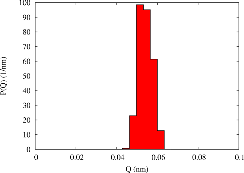
Figure 1: Probability density for the radial coordinate $Q$.

The puckering free energy profile calculated using the $\theta$ and $\phi$ CVs is presented in Fig.2. The full CV space has been spanned by the metadynamics run, and a deep rift can be observed at $\theta\simeq 0$, which contains the global minimum corresponding to the ⁴C₁ conformation around $\phi=0$ and some slightly distorted chairs around $\phi=\pi/2$ and $3\pi/2$. The next conformer which can be observed is a ^O,3B close to the border of the diagram, at $\theta\simeq\pi/2$ and $\phi\simeq 0$. In the middle of the diagram ($\theta\simeq\pi/2,\phi\simeq\pi$) a local minimum corresponding to the B_O,3 conformer is present. A steep barrier then has to be overome, right after the equatorial line, to reach the ¹C₄ conformation, the inverted chair, located at around $\theta\simeq\pi$.

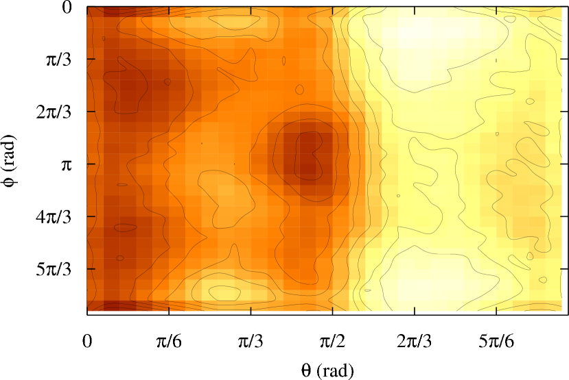
Figure 2: Puckering free energy profile calculated using polar coordinates $(\theta,\phi)$. Every isoline corresponds to an increment in energy of 5 kJ/mol. (Darker colors correspond to lower energies).

By employing the polar coordinates, the exploration of the southern hemisphere was not a problem, and the barrier which has been found located close to the equatorial line is definitely high ($\simeq 40$ kJ/mol), but easily surmountable with the metadynamics technique. On the contrary, the problem of ergodicity is evident if one employs Cartesian coordinates to perform the metadynamics exploration. Since the $q_{x}$ and $q_{y}$ coordinates alone can not distinguish between northern and southern hemisphere, we tracked the value of $\cos(\theta)$, and were thus able to compute (see Fig.3) the free energy landscape as well as the distribution of the Gaussians placed in either of the two hemispheres. It should be noted that the free energy $G$ is a logarithmic measure of the number of conformations $s$ visited during the metadynamics run: $G(s)\simeq\log\left[\int\delta_{s,s(t^{\prime})}\mathrm{d}t^{\prime}\right]$. Therefore, the plots obtained by separating out the contributions $G^{\pm}(s)\simeq\log\left[\int\delta_{s,s(t^{\prime})}H(\pm\cos(\theta))\mathrm{d}t^{\prime}\right]$ of the conformations in the northern and southern hemisphere, respectively, are only indicative of the sampled regions (here $H$ denotes the Heavside function). The two contributions $G^{\pm}$ are not to be considered as free energies and, in particular, they do not add up to the real free energy landscape: $G(s)\neq G^{+}(s)+G^{-}(s)$. Nevertheless, the contributions from the two hemispheres are quite informative, and the first thing one notices from their graphs (see Fig. 3, middle and bottom panels) is that only the northern hemisphere has been explored completely during the metadynamics run. This result qualitatively reproduces the behavior observed by Biarnés and coworkersBiarnes et al. (2007), who noticed a sampling of the northern hemisphere only, and attributed to the presence of an extremely high free energy barrier at the equatorial line.

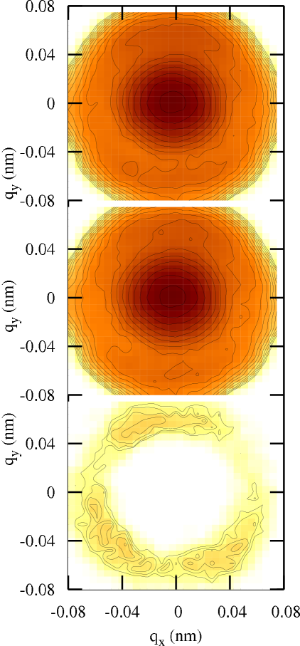
Figure 3: Top panel: free energy profile generated using the $q_{x}$,$q_{y}$ pair of CVs. Middle and bottom panels: logarithm of the distribution of the Gaussians placed in the northern ($G^{+}$) and southern ($G^{-}$) hemispheres, respectively, during the metadynamics run. Every isoline corresponds to an increment in energy of 5 kJ/mol. Note that the figures in the middle and bottom panels do not have not the meaning of a free energy; in these cases isolines have to be understood only as a guide to the eye.

	4C1	1C4	O,3B	BO,3
$\Delta G^{\dagger}$	0.0	27.7	9.3	20.0
$(\theta,\phi)$	(0.2,6.1)	(2.9,6.1)	(1.4,0.0)	(1.5,3.4)
$\Delta G^{\ddagger}$	0.0	n.a.	28.7	33.1
$(q_{x},q_{y})$	(0.0,0.0)	n.a.	(0.5,5.9)	(-0.5,-6.4)

Table 1: The free energy ($\Delta G$, in kJ/mol) of different conformations, estimated using the two different sets of Cartesian^† and polar^‡ coordinates, along with the location of the conformations on the ($\theta,\phi$) plane (in rad) and ($q_{x},q_{y}$) plane (in $10^{-2}$nm), respectively.

During our metadynamics run, the southern hemisphere was reached thanks to natural fluctuations, but the sampled region is relatively small, and the metadynamics algorithm was definitely not able to be ergodic, even though a tenfold longer simulation time and the same Gaussian heights have been used with respect to the metadynamics with polar coordinates. For comparison, the estimate of the barrier height at the equatorial line obtained using Cartesian coordinate is more than 90 kJ/mol, compared with the value of about 40 kJ/mol estimated using polar coordinates. The presence of this artefact, as discussed in Section II, prevents the system from exploring the southern hemisphere properly and the metadynamics from being ergodic. The magnitude of the bias which is introduced by using Cartesian coordinates can be appreciated by looking at the differences in energy of some selected conformations with that of the ¹C₄ chair, presented in Tab.1.

Figure 4: Bivariate distribution $P(q_{r},Q)$ of the projection $q_{r}=\sqrt{q_{x}^{2}+q_{y}^{2}}=Q\sin(\theta)$ versus the total puckering amplitude $Q$ during a metadynamics run using $q_{x}$ and $q_{y}$ as CVs. A strong correlation develops as the $q_{r}/Q=sin(\theta)=1$ line is approached (Lighter colors correspond to lower probabilities).

The extent of the artefacts introduced by the use of Cartesian CVs can also be appreciated by looking at the effect that the mixing of tangent and radial coorinates has on the range of sampled conformations at different $Q$. In Fig.4 the correlation between $Q$ and the magnitude of the projected puckering vector $q_{r}\equiv\sqrt{q_{x}^{2}+q_{y}^{2}}$ is presented. At low values of $q_{r}$, that is, at low values of the zenithal angle $\theta$, the correlation with $Q$ is minimal, and the radial coordinate is distributed around the value of 0.055 as in the free case. At values of $q_{r}$ larger than 0.05, on the other hand, a strong correlation develops, which almost completely correlates the two variables along the $q_{r}/Q=\sin(\theta)=1$ line. This means that when the system is driven close to the equatorial line by the metadynamics, conformations that are sampled at higher values of $\theta$ are necessarily characterized by an unphysically high total puckering amplitude, strongly biasing the reconstructed free energy profile.

IV Conclusions

We have critically investigated the use of two different sets of CVs which can be used for the study of puckered conformations of cyclic compounds. In this work we have shown that the Cartesian and polar sets of coordinates are not equivalent, and that only the polar one is a proper set of CVs that allows the ergodic and unbiased sampling of the space of different puckered conformations for six-membered rings. We supported our conclusions by performing a metadynamics calculation of the puckering free energy surface of a glucuronic acid ring, described by a simple atomistic model in vacuo using the gromos G45A4 force-field. We showed how the metadynamics performed using Cartesian CVs – in contrast to the polar case – is non-ergodic, and how the reconstructed free energy profile suffers from strong biases. The conformations sampled close to the equatorial line had unphysical values of the total puckering amplitude, which has been shown to be markedly correlated with the proximity to the equatorial line.

In conclusion, the non-ergodicity and the biases are too high a price to be paid for the simplifications deriving from the use of Cartesian coordinates to represent puckered conformations. To the best of our knowledge, only the Cartesian variant has been employed so farBiarnes et al. (2007) as a CV set for an accelerated sampling method, namely, metadynamics. In contrast, our analysis suggests that only polar coordinates should be considered as a proper set of CVs when studying the puckered conformations of ring structures via enhanced sampling techniques such as metadynamics.

Appendix: Gradients of the puckering coordinates

For a metadynamics run it is necessary to compute gradients of the CVs, in order to include the bias contribution to the force acting on the system. To perform this task in this case it is necessary to recall some details in puckering coordinates construction.

The starting point are the position vectors $\mathbf{r}_{j}$ (here the index $j$ runs from 1 to an arbitrary $N$) of the atoms of the ring, with respect to an arbitrary reference frame in which we will compute derivatives. From these vectors it is possible to calculate the geometrical center of the ring $\mathbf{R}=\frac{1}{N}\sum_{j}\mathbf{r}_{j}$ and use this point as the origin of a new reference frame for the system, in which the atomic coordinate will be (summation on repeated indices is implied)

$$\mathbf{R}_{j}=\mathbf{r}_{j}-\mathbf{R}=\mathbf{r}_{i}\Delta_{ij}\;\;,\;\;\Delta_{ij}=\delta_{ij}-1/N$$ (5)

($i=1,\ldots,N$, and $\delta_{ij}$ is the Kronecker symbol). In order to build all puckering coordinates the projections $z_{j}=\mathbf{R}_{j}\cdot\hat{\mathrm{n}}$ onto the mean plane axis $\hat{\mathrm{n}}$ are required. The mean plane axis can be univocally defined as Cremer and Pople (1975)

$$\hat{\mathrm{n}}=\frac{\mathbf{R}^{\prime}\times\mathbf{R}^{\prime\prime}}{|\mathbf{R}^{\prime}\times\mathbf{R}^{\prime\prime}|}\quad,\left\{\begin{array}[]{l}\mathbf{R}^{\prime}=\sum_{j}\mathbf{R}_{j}w_{1,j}\vskip 3.0pt plus 1.0pt minus 1.0pt\\ \mathbf{R}^{\prime\prime}=\sum_{j}\mathbf{R}_{j}v_{1,j}\end{array}\right.$$ (6)

where the symbols

$$w_{m,j}=\sin\frac{2\pi m(j-1)}{N}\;,\;v_{m,j}=\cos\frac{2\pi m(j-1)}{N}$$ (7)

are defined here for further use.

The general puckering coordinate can now be rewritten as an explicit function of the atomic projections as

$$\left\{\begin{array}[]{l}q_{m}=\sqrt{2/N}\sqrt{\mathscr{A}_{m}^{2}+\mathscr{B}_{m}^{2}}\vskip 3.0pt plus 1.0pt minus 1.0pt\\ \phi_{m}=\arctan\big{[}-\mathscr{A}_{m}/\mathscr{B}_{m}\big{]}\vskip 3.0pt plus 1.0pt minus 1.0pt\\ q_{N/2}=\sqrt{1/N}\mathscr{C}\quad,\end{array}\right.$$ (8)

making use of the definitions

$$\mathscr{A}_{m}=z_{j}w_{m,j}\;,\;\;\mathscr{B}_{m}=z_{j}v_{m,j}\;,\;\;\mathscr{C}=z_{j}(-1)^{j-1}$$ (9)

to simplify the notation. All puckering coordinates are eventually a function of the projections $z_{j}$, whose gradient is

$$\nabla_{i}z_{j}=\nabla_{i}\left[\frac{\mathbf{R}_{j}\cdot(\mathbf{R}^{\prime}\times\mathbf{R}^{\prime\prime})}{|\mathbf{R}^{\prime}\times\mathbf{R}^{\prime\prime}|}\right]$$

$$=\frac{-z_{j}\nabla_{i}\left|\mathbf{R}^{\prime}\times\mathbf{R}^{\prime\prime}\right|^{2}}{2|\mathbf{R}^{\prime}\times\mathbf{R}^{\prime\prime}|^{2}}+\frac{\nabla_{i}\left[\mathbf{R}_{j}\cdot(\mathbf{R}^{\prime}\times\mathbf{R}^{\prime\prime})\right]}{|\mathbf{R}^{\prime}\times\mathbf{R}^{\prime\prime}|}.$$ (10)

Noting that $\nabla_{i}(\mathbf{R}_{j}\cdot\hat{e}_{\alpha})=\Delta_{ij}\hat{\mathrm{e}}_{\alpha}$ (with $\hat{e}_{\alpha}$ an element of the vector basis) after a somewhat long but straightforward calculation the terms of the right member in Eq.(10) can be evaluated to be

$$\begin{array}[]{ll}\nabla_{i}\left|\mathbf{R}^{\prime}\times\mathbf{R}^{\prime\prime}\right|^{2}&=2\Delta_{ik}w_{1,k}\big{[}\mathbf{R}^{\prime}|\mathbf{R}^{\prime\prime}|^{2}-\mathbf{R}^{\prime\prime}(\mathbf{R}^{\prime\prime}\cdot\mathbf{R}^{\prime})\big{]}+\\ &+2\Delta_{ik}v_{1,k}\big{[}\mathbf{R}^{\prime\prime}|\mathbf{R}^{\prime}|^{2}-\mathbf{R}^{\prime}(\mathbf{R}^{\prime\prime}\cdot\mathbf{R}^{\prime})\big{]}\end{array}$$

and

$$\begin{array}[]{ll}\nabla_{i}\big{[}\mathbf{R}_{j}\cdot(\mathbf{R}^{\prime}\times\mathbf{R}^{\prime\prime})\big{]}&=\Delta_{ij}\mathbf{R}^{\prime}\times\mathbf{R}^{\prime\prime}+\Delta_{ik}w_{1,k}\mathbf{R}^{\prime\prime}\times\mathbf{R}_{j}+\\ &\quad+\Delta_{ik}v_{1,k}\mathbf{R}_{j}\times\mathbf{R}^{\prime}.\end{array}$$

References

- Kilpatrick et al. (1947) J. E. Kilpatrick, K. S. Pitzer, and R. Spitzer, J. Am. Chem. Soc. 64, 2483 (1947).
- Cremer and Pople (1975) D. Cremer and J. A. Pople, J. Am. Chem. Soc. 97 (1975).
- Boessenkool and Boeyens (1980) I. Boessenkool and J. Boeyens, J. Chem. Crystallogr. 10, 11 (1980).
- Evans and Boeyens (1988) D. Evans and J. Boeyens, Acta Cryst. B44, 663 (1988).
- Evans and Boeyens (1990) D. G. Evans and J. C. A. Boeyens, Acta Cryst. B46, 524 (1990).
- Strauss and Pickett (1971) H. L. Strauss and H. M. Pickett, J. Chem. Phys. p. 324 (1971).
- Boeyens and Evans (1989) J. C. A. Boeyens and D. G. Evans, Acta Cryst. B45, 577 (1989).
- Strauss and Pickett (1970) H. L. Strauss and H. M. Pickett, J. Am. Chem. Soc. 92, 7281 (1970).
- Torrie and Valleau (1977) G. Torrie and J. Valleau, J. Comput. Phys. 23, 187 (1977).
- Bartels and Karplus (1997) C. Bartels and M. Karplus, J. Comput. Chem. 18, 1450 (1997).
- Laio and Parrinello (2002) A. Laio and M. Parrinello, Proc. Natl. Acad. Sci. USA (2002).
- Bussi et al. (2006) G. Bussi, A. Laio, and M. Parrinello, Phys. Rev. Lett. (2006).
- Laio and Gervasio (2008) A. Laio and F. L. Gervasio, Rep. Prog. Phys. 71, 126601 (2008).
- Appell et al. (2004) M. Appell, G. Strati, J. Willett, and F. Momany, Carbohydr. Res. 339, 537 (2004).
- Biarnes et al. (2007) X. Biarnes, A. Ardevol, A. Planas, C. Rovira, A. Laio, and M. Parrinello, J. Am. Chem. Soc. 129, 10686 (2007).
- Lins and Hunenberger (2005) R. Lins and P. Hunenberger, J. Comp. Chem. 26 (2005).
- Barducci et al. (2008) A. Barducci, G. Bussi, and M. Parrinello, Phys. Rev. Lett. 100, 020603 (pages 4) (2008).
- Camilloni et al. (2008) C. Camilloni, D. Provasi, G. Tiana, and R. A. Broglia, Proteins 71, 1647 (2008).
- Berendsen et al. (1995) H. J. C. Berendsen, D. van der Spoel, and R. van Drunen, Comp. Phys. Comm. 91, 43 (1995).
- Lindahl et al. (2001) E. Lindahl, B. Hess, and D. van der Spoel, J. Mol. Mod. 7, 306 (2001).