Average and deviation for slow-fast stochastic partial differential equations

Abstract

Averaging is an important method to extract effective macroscopic dynamics from complex systems with slow modes and fast modes. This article derives an averaged equation for a class of stochastic partial differential equations without any Lipschitz assumption on the slow modes. The rate of convergence in probability is obtained as a byproduct. Importantly, the deviation between the original equation and the averaged equation is also studied. A martingale approach proves that the deviation is described by a Gaussian process. This gives an approximation to errors of $\mathcal{O}(\epsilon)$ instead of $\mathcal{O}(\sqrt{\epsilon})$ attained in previous averaging.

Keywords:   Slow-fast stochastic partial differential equations, averaging, martingale

1 Introduction

The need to quantify uncertainties is widely recognized in modeling, analyzing, simulating and predicting complex phenomena [5, 10, 14, e.g.]. Stochastic partial differential equations (spdes) are appropriate mathematical models for many multiscale systems with uncertain influences [17].

Very often a complex system has two widely separated timescales. Then a simplified equation which governs the evolution of the system over the long time scale is highly desirable. Such a simplified equation, capturing the dynamics of the system at the slow time scale, is often called an averaged equation. There is a great deal work on averaging principles for deterministic ordinary differential equations [1, 2, 15, e.g.] and for stochastic ordinary differential equations [6, 8, 9, e.g.]. But there are few results on the averaging principle for spdes. Recently, an averaged equation for a system of reaction-diffusion equations with stochastic fast component was obtained by a Lipschitz assumption on all nonlinear terms [4]. The resultant averaged equation is deterministic.

This article derives an averaged equation for a class of spdes with stochastic fast component and proves a square-root rate of convergence in probability. Furthermore, the deviation between the original system and the averaged system is determined.

Let $D$ be an open bounded interval and $L^{2}(D)$ be the Lebesgue space of square integrable real valued functions on $D$. Consider the following slow-fast system

$$du^{\epsilon} = \big{[}\Delta u^{\epsilon}+f(u^{\epsilon},v^{\epsilon})\big{]}\,dt+\sigma_{1}\,dW_{1}(t)\,,\quad u^{\epsilon}(0)=u_{0}\in L^{2}(D)\,,$$ (1)

$$dv^{\epsilon} = \frac{1}{\epsilon}\big{[}\Delta v^{\epsilon}+g(u^{\epsilon},v^{\epsilon})\big{]}\,dt+\frac{\sigma_{2}}{\sqrt{\epsilon}}\,dW_{2}(t)\,,\quad v^{\epsilon}(0)=v_{0}\in L^{2}(D)\,,$$ (2)

with Dirichlet boundary condition. Here $W_{1}$ and $W_{2}$ are mutually independent $L^{2}(D)$ valued Wiener processes defined on a complete probability space $(\Omega,\mathcal{F},{\mathbb{P}})$ detailed in the following section. If for any fixed $u$, the fast system (2) has unique invariant measure $\mu_{u}$, then as $\epsilon\rightarrow 0$ , under some conditions, the solution $u^{\epsilon}$ of (1), converges in probability to the solution of

$$du = \big{[}\Delta u+\bar{f}(u)\big{]}\,dt+\sigma_{1}\,dW_{1}(t)\,,$$ (3)

$$u(0) = u_{0}\quad\text{and}\quad u|_{\partial D}=0\,.$$ (4)

Here, the average

$$\bar{f}(u)=\int_{H}f(u,v)\mu_{u}(dv)\,.$$ (5)

And the convergence rate is proved to be $1/2$ in the following sense for any $\kappa>0$

$$\mathbb{P}\Big{\{}\sup_{0\leq t\leq T}|u^{\epsilon}(t)-u(t)|\leq C^{\kappa}_{T}\epsilon^{1/2}\Big{\}}>1-\kappa$$ (6)

for some positive constant $C^{\kappa}_{T}$; see Section 4.

Furthermore by estimate (6), as $\epsilon\rightarrow 0$ the limit of $(u^{\epsilon}(t)-u(t))/\sqrt{\epsilon}$ is proved to be a Gaussian process; see Section 5.

We stress that Theorem 3 gives a much better approximation than the averaged equation.

2 Preliminaries and main results

Let $H=L^{2}(D)$ with $L^{2}$-norm denoted by $|\cdot|$ and inner product by $\langle\cdot,\cdot\rangle$. Define the abstract operator $A=\Delta$ with zero Dirichlet boundary condition which defines a compact analytic semigroup $e^{At}$, $t\geq 0$ on $H$. For any $\alpha>0$ , $u\in H$ define $|u|_{\alpha}=|A^{\alpha/2}u|$ and for $\alpha=1$ , the norm is denoted as $\|\cdot\|$. Then let $H_{0}^{\alpha}$ be the space the closure of $C_{0}^{\infty}(D)$, the space of smooth functions with compact support on $D$, under the norm $|\cdot|_{\alpha}$ . Furthermore, let $H^{-\alpha}$ denote the dual space of $H_{0}^{\alpha}$ and denote by $\lambda_{1}$ the first eigenvalue of $A$ . Also we are given $H$ valued Wiener processes $W_{1}(t)$ and $W_{2}(t)$, $t\geq 0$ , which are mutually independent on the complete probability space $(\Omega,\mathcal{F},\mathcal{F}_{t},{\mathbb{P}})$ [12]. Denote by $\mathbb{E}$ the expectation operator with respect to ${\mathbb{P}}$. Then consider the following spdes with separated time scale

$$du^{\epsilon} = \big{[}Au^{\epsilon}+f(u^{\epsilon},v^{\epsilon})\big{]}\,dt+\sigma_{1}\,dW_{1}\,,\quad u^{\epsilon}(0)=u_{0}\in H\,,$$ (7)

$$dv^{\epsilon} = \frac{1}{\epsilon}\big{[}Av^{\epsilon}+g(u^{\epsilon},v^{\epsilon})\big{]}\,dt+\frac{\sigma_{2}}{\sqrt{\epsilon}}\,dW_{2}\,,\quad v^{\epsilon}(0)=v_{0}\in H\,.$$ (8)

Here $\sigma_{1}\in{\mathbb{R}}\,,\sigma_{2}\neq 0$ are arbitrary real numbers. For our purpose we adopt the following four hypotheses.

H₁

$f(x,y):{\mathbb{R}}\times{\mathbb{R}}\rightarrow{\mathbb{R}}$ is continuous, there is a positive constant $C_{f}$, such that $f^{\prime}_{x}(x,y)\leq C_{f}$ , $|f^{\prime}_{y}(x,y)|\leq C_{f}$ and that for any $x,y$

$$|f(x,y)|^{2}\leq ax^{6}+by^{2}+c\,,$$

$$f(x,y)x\leq-ax^{2}-bxy+c\,,$$

$$(f(x_{1},y)-f(x_{2},y))(x_{1}-x_{2})\leq a(x_{1}-x_{2})^{2}+c\,,$$

for some positive constants $a$, $b$ and $c$.

H₂

$g(x,y):{\mathbb{R}}\times{\mathbb{R}}\rightarrow{\mathbb{R}}$ is continuous and is Lipschitz with respect to the both variables with Lipschitz constant $C_{g}$. For any $x,y$

$$g(x,y)y\leq-dy^{2}+exy$$

for some positive constants $d$ and $e$.

H₃

$b\geq e$ and $C_{g}<\lambda_{1}$ .

H₄

$W_{1}$ and $W_{2}$ are Q-Wiener processes with covariance operator $Q_{1}$ and $Q_{2}$ respectively. Moreover, $\operatorname{tr}[A^{1/2}Q_{i}]<\infty$ , $i=1,2$ .

With the above assumptions we have the first result on the fast component that is proved at the end of Section 3.

Theorem 1.

Assume H₁–H₄. For any fixed $u\in H$ , system (2) has a unique stationary solution, $\eta_{u}^{\epsilon}(t)$, with distribution $\mu_{u}$ independent of $\epsilon$. Moreover, the stationary measure $\mu_{u}$ is exponentially mixing.

Then we prove the following averaging result.

Theorem 2.

Assume H₁–H₄. Given $T>0$ , for any $u_{0}\in H$ , solution $u^{\epsilon}(t,u_{0})$ of (1) converges in probability to $u$ in $C(0,T;H)$ which solves (3)–(4). Moreover the convergence rate is $1/2$ that is for any $\kappa>0$

$$\mathbb{P}\Big{\{}\sup_{0\leq t\leq T}|u^{\epsilon}(t)-u(t)|\leq C^{\kappa}_{T}\sqrt{\epsilon}\Big{\}}>1-\kappa$$

for some positive constant $C^{\kappa}_{T}>0$ .

Having the above averaging result we consider the deviation between $u^{\epsilon}$ and $u$. For this we introduce

$$z^{\epsilon}(t)=\frac{1}{\sqrt{\epsilon}}(u^{\epsilon}-u)\,.$$ (9)

Then we have

Theorem 3.

$z^{\epsilon}$ converges in distribution to $z$ in space $C(0,T;H)$ which solves

$$\dot{z}=Az+\overline{f^{\prime}_{u}}(u)z+\sqrt{B(u)}\dot{\overline{W}}$$ (10)

where $B(u):H\rightarrow H$ is Hilbert–Schmidt with

$$B(u)=2\int_{0}^{\infty}\mathbb{E}\Big{[}(f(u,\eta_{u}(t))-\bar{f}(u))\otimes(f(u,\eta_{u}(0))-\bar{f}(u))\Big{]}dt$$

$$\overline{f^{\prime}_{u}}(u)=\int_{H}f^{\prime}_{u}(u,v)\mu^{u}(dv)$$

and $\overline{W}(t)$ is an $H$-valued cylindrical Wiener process with covariance operator $\text{Id}_{H}$.

3 Some a priori estimates

This section gives some a priori estimates for the solution of (7)–(8) which yields the tightness of $u^{\epsilon}$ in space $C(0,T;H)$. First we give a wellposedness result.

Theorem 4.

Assume H₁–H₄. For any $u_{0}\in H$ , $v_{0}\in H$ and any $T>0$ , there is unique solution $(u^{\epsilon}(t),v^{\epsilon}(t))$ in $L^{2}(\Omega,C(0,T;H)\cap L^{2}(0,T;H^{1}_{0}))$ for (7)–(8) .

The above result is derived by a standard method [12] and so is here omitted. Then we have the following estimates for $(u^{\epsilon},v^{\epsilon})$.

Theorem 5.

Assume H₁–H₄. For $u_{0}\in H^{1}_{0}$ and $v_{0}\in H_{0}^{1}$ , for any $T>0$ , there is a positive constant $C_{T}$ which is independent of $\epsilon$, such that

$$\mathbb{E}\sup_{0\leq t\leq T}\|u^{\epsilon}(t)\|^{2}+\sup_{0\leq t\leq T}\mathbb{E}|v^{\epsilon}(t)|^{2}\leq C_{T}(\|u_{0}\|^{2}+|v_{0}|^{2})$$ (11)

and for any positive integer $m$,

$$\mathbb{E}\int_{0}^{T}\|u^{\epsilon}(s)\|^{2m}ds+\mathbb{E}\int_{0}^{T}\|v^{\epsilon}(t)\|^{2}ds\leq C_{T}(|u_{0}|^{2}+|v_{0}|^{2})\,.$$ (12)

Moreover

$$\mathbb{E}|\dot{u}^{\epsilon}|_{L^{2}(0,T;H^{-1})}\leq C_{T}(|u_{0}|^{2}+|v_{0}|^{2})\,.$$ (13)

Proof.

Applying Itô formula to $|u^{\epsilon}(t)|^{2}$ and $|v^{\epsilon}(t)|^{2}$ respectively and by Gronwall lemma there is positive constant $C$ which is independent of $\epsilon$ such that for any $t>0$

$$\mathbb{E}|u^{\epsilon}(t)|^{2}+\epsilon\mathbb{E}|v^{\epsilon}(t)|^{2}\leq C(|u_{0}|^{2}+|v_{0}|^{2})\,.$$ (14)

At the same time we have for any $T>0$ that there is positive constant $C_{T}$ which is independent of $\epsilon$ such that for $0\leq t\leq T$

$$\mathbb{E}\int_{0}^{t}\|u^{\epsilon}(s)\|^{2}ds+\mathbb{E}\int_{0}^{t}\|v^{\epsilon}(s)\|^{2}ds\leq C_{T}(|u_{0}|^{2}+|v_{0}^{2}|)$$ (15)

and

$$\sup_{t\geq 0}\mathbb{E}|v^{\epsilon}(t)|^{2}\leq C(|u_{0}|^{2}+|v_{0}|^{2})\,.$$ (16)

By applying Itô formula to $\|u^{\epsilon}(t)\|^{2}$ and using (15), a lemma of Da Prato & Zabczyk’s [12, Lemma 7.2] proves

$$\mathbb{E}\sup_{0\leq t\leq T}\|u^{\epsilon}(t)\|^{2}\leq C_{T}(\|u_{0}\|^{2}+|v_{0}|^{2})\,.$$ (17)

Further, applying Itô formula to $\|u^{\epsilon}(t)\|^{2m}$ and $\|v^{\epsilon}(t)\|^{2m}$, by the assumption on $f$ and (15), we then establish the inequality (12). The bound (13) can be proved by estimating (12) and the embedding $H^{1}_{0}\subset L^{6}(D)$. ∎

Now we show that $\mathcal{L}(u^{\epsilon})$, the distribution of $u^{\epsilon}$, is tight in $C(0,T;H)$. For this we need the following lemma by Simon [13].

Lemma 6.

Let $E$, $E_{0}$ and $E_{1}$ be Banach spaces such that $E_{1}\Subset E_{0}$ , the interpolation space $(E_{0},E_{1})_{\theta,1}\subset E$ with $\theta\in(0,1)$ and $E\subset E_{0}$ with $\subset$ and $\Subset$ denoting continuous and compact embedding respectively. Suppose $p_{0},p_{1}\in[1,\infty]$ and $T>0$ , such that

$$\mathcal{V}\text{ is a bounded set in }L^{p_{1}}(0,T;E_{1})$$

and

$$\partial\mathcal{V}:=\{\partial v:v\in\mathcal{V}\}\text{ is a bounded set in }L^{p_{0}}(0,T;E_{0}).$$

Here $\partial$ denotes the distributional derivative. If $1-\theta>1/p_{\theta}$ with

$$\frac{1}{p_{\theta}}=\frac{1-\theta}{p_{0}}+\frac{\theta}{p_{1}}\,,$$

then $\mathcal{V}$ is relatively compact in $C(0,T;E)$.

By the above lemma we have the following result.

Theorem 7.

Assume H₁–H₄. $\{\mathcal{L}(u^{\epsilon})\}_{\epsilon>0}$ is tight in space $C(0,T;H)$.

Proof.

Taking $E_{0}=H^{-1}$, $E=H$ and $E_{1}=H_{0}^{1}$ and $p_{0}=2$ , $\theta=1/2$ . By Theorem 5, $p_{1}$ can be taken as arbitrary lager positive integer, then by Lemma 6, $\{\mathcal{L}(u^{\epsilon})\}_{\epsilon>0}$ is tight in space $C(0,T;H)$. ∎

Proof of Theorem 1.

For any two solutions $v_{1}^{\epsilon}$ and $v_{2}^{\epsilon}$, the Itô formula yields

$$\mathbb{E}|v_{1}^{\epsilon}(t)-v_{2}^{\epsilon}(t)|^{2}\leq e^{-2(\lambda_{1}-C_{g})t/\epsilon}\mathbb{E}|v_{1}(0)-v_{2}(0)|\,,$$

which means the existence of a unique stationary solution $\eta_{u}^{\epsilon}$ for (8) distributes as $\mu_{u}$ such that for any $v_{0}\in H$

$$\mathbb{E}|v^{\epsilon}(t)-\eta^{\epsilon}_{u}(t)|^{2}\leq e^{-2(\lambda_{1}-C_{g})t/\epsilon}\mathbb{E}|v_{0}-\eta_{u}^{\epsilon}(0)|^{2}\,,$$ (18)

which yields the exponential mixing. Moreover, since $|f^{\prime}_{y}(x,y)|\leq C_{f}$ , we also have

$$\mathbb{E}\Big{|}f(u,v^{\epsilon}(t))-\int_{H}f(u,x)\mu_{u}(dx)\Big{|}\leq C(1+|v_{0}|^{2})e^{-2(\lambda_{1}-C_{g})t/\epsilon}\,.$$ (19)

By the time scale transformation $t\rightarrow\tau=\epsilon t$ , (8) is transformed to

$$dv=\big{[}Av+g(u,v)\big{]}\,d\tau+\sigma_{2}\,d\tilde{W}_{2}(\tau)\,,\quad v(0)=v_{0}\,,$$ (20)

where $\tilde{W}_{2}$ is the scaled version of $W_{2}$ and with the same distribution. Then the spde (20) has a unique stationary solution $\eta_{u}$ with distribution $\mu_{u}$. And by the ergodic property of $\mu_{u}$, we have

$$\bar{f}(u)=\lim_{t\rightarrow\infty}\frac{1}{t}\int_{0}^{t}f(u,\eta_{u}(s))\,ds\,.$$ (21)

Furthermore, by a generalized theorem on contracting maps depending on a parameter [3, Appendix C], [4], $v_{u}(t)$ is differential with respect $u$ with

$$\sup_{u,v_{0}\in H,\ 0\leq t<\infty}|D_{u}v_{u}|_{\mathcal{L}(H)}\leq C$$ (22)

for some positive constant $C$ . ∎

We end this section by giving the following a priori estimates on the solutions of the averaged equation (3)–(4) . First we need a local Lipschitz property of $\bar{f}$ which is yielded by (22) and the following estimate, for any $u_{1}$ , $u_{1}\in H_{0}^{1}$

$$\frac{1}{\tau}\Big{|}\int_{0}^{\tau}[f(u_{1},v_{u_{1}}(s))-f(u_{2},v_{u_{2}}(s))\big{]}ds\Big{|}_{H}$$ (23)

$$\leq \frac{1}{\tau}\Big{|}\int_{0}^{\tau}[f(u_{1},v_{u_{1}}(s))-f(u_{2},v_{u_{1}}(s))\big{]}ds\Big{|}_{H}$$

$${}+\frac{1}{\tau}\Big{|}\int_{0}^{\tau}[f(u_{2},v_{u_{1}}(s))-f(u_{2},v_{u_{2}}(s))\big{]}ds\Big{|}_{H}$$

$$\leq 2\Big{[}\|u_{1}\|^{2}+\|u_{2}\|^{2}+\sup_{u,v_{0}\in H,\ 0\leq t<\infty}|D_{u}v(t)|_{\mathcal{L}(H)}\Big{]}|u_{1}-u_{2}|\,.$$

Lemma 8.

Assume $\textbf{H}_{1}$–$\textbf{H}_{4}$ . For any $u_{0}\in H_{0}^{1}$, for any $T>0$, (3)–(4) has a unique solution $u\in L^{2}(\Omega,C(0,T;H)\cap L^{2}(0,T;H_{0}^{1}))$ . Moreover there is a positive constant $C_{T}$ such that for any positive integer $m\geq 2$ and any $0\leq t\leq T$

$$\mathbb{E}\|u(t)\|^{m}\leq C_{T}(1+\|u_{0}\|^{m})\,.$$ (24)

Proof.

Applying Itô formula to $|u(t)|^{2}$ yields

$$\frac{1}{2}\frac{d}{dt}|u(t)|^{2}=-\|u(t)\|^{2}+\langle\bar{f}(u(t)),u(t)\rangle+\sigma_{1}\langle u(t),\dot{W}_{1}\rangle+\frac{\sigma_{1}^{2}}{2}\operatorname{tr}Q_{1}\,.$$

By (21) and assumption $\textbf{H}_{1}$

$$\langle\bar{f}(u(t)),u(t)\rangle = \lim_{s\rightarrow\infty}\frac{1}{s}\int_{0}^{s}\big{\langle}f(u(t),\eta_{u(t)}(\tau)),u(t)\big{\rangle}\,d\tau$$

$$\leq -a|u(t)|^{2}-b\langle\bar{\eta}_{u(t)},u(t)\rangle+c\,.$$

Then by the Gronwall lemma and (16) there is some positive constant $C$ such that for any $t>0$

$$\mathbb{E}|u(t)|^{2}\leq C(1+|u_{0}|^{2})\,.$$

Now by the same analysis of the proof of Theorem 5 we obtain (24) . Then by the above a priori estimates and the local Lipschitz property of $\bar{f}$, a standard method [12] yields the existence and uniqueness of $u$. ∎

4 Averaged equation

This section gives the averaged equation and, as a byproduct, the convergence rate is obtained. For this we consider our system in a smaller probability space. By Theorem 7, for any $\kappa>0$ there is compact set $K_{\kappa}$ in $C(0,T;H)$ such that

$${\mathbb{P}}\{u^{\epsilon}\in K_{\kappa}\}>1-\kappa\,.$$

Here $K_{\kappa}$ is chosen as a family of decreasing sets with respect to $\kappa$. Moreover, by the estimate (11) and Markov inequality, we further choose the set $K_{\kappa}$ such that for $u^{\epsilon}\in K_{\kappa}$

$$\|u^{\epsilon}(t)\|^{2}\leq C_{T}^{\kappa}\,,\quad t\in[0,T]\,,$$

for some positive constant $C_{T}^{\kappa}$.

Proof of Theorem 2.

Now we prove the rate of convergence. In order to do this, for any $\kappa>0$ we introduce a new sub-probability space $(\Omega_{\kappa},\mathcal{F}_{\kappa},{\mathbb{P}}_{\kappa})$ defined by

$$\Omega_{\kappa}=\{\omega\in\Omega:u^{\epsilon}(\omega)\in K_{\kappa}\}\,,\quad\mathcal{F}_{\kappa}=\{S\cap\Omega_{\kappa}:S\in\mathcal{F}\}$$

and

$${\mathbb{P}}_{\kappa}(S)=\frac{{\mathbb{P}}(S\cap\Omega_{\kappa})}{{\mathbb{P}}(\Omega_{\kappa})}\quad\text{for}\quad S\in\mathcal{F}_{\kappa}\,.$$

Then ${\mathbb{P}}(\Omega\setminus\Omega_{\kappa})\leq\kappa$ . In the following we denote by $\mathbb{E}_{\kappa}$ the expectation operator with respect to ${\mathbb{P}}_{\kappa}$.

Now we restrict $\omega\in\Omega_{\kappa}$ and introduce an auxiliary process. For any $T>0$ , partition the interval $[0,T]$ into subintervals of length $\delta=\sqrt{\epsilon}$ . Then we construct processes $(\tilde{u}^{\epsilon},\tilde{v}^{\epsilon})$ such that for $t\in[k\delta,(k+1)\delta)$,

$$\tilde{u}^{\epsilon}(t) = e^{A(t-k\delta)}u^{\epsilon}(k\delta)+\int_{k\delta}^{t}e^{A(t-s)}f(u^{\epsilon}(k\delta),\tilde{v}^{\epsilon}(s))\,ds$$ (25)

$${}+\sigma_{1}\int_{k\delta}^{t}e^{A(t-s)}dW_{1}(s)\,,\quad\tilde{u}^{\epsilon}(0)=u_{0}$$

$$d\tilde{v}^{\epsilon}(t) = \frac{1}{\epsilon}\big{[}B\tilde{v}^{\epsilon}(t)+g(u^{\epsilon}(k\delta),\tilde{v}^{\epsilon}(t))\big{]}\,dt+\frac{\sigma_{2}}{\sqrt{\epsilon}}\,dW_{2}(t)\,,$$ (26)

$$\tilde{v}^{\epsilon}(k\delta)=v^{\epsilon}(k\delta)\,.$$

By the Itô formula for $t\in[k\delta,(k+1)\delta)$

$$\frac{1}{2}\frac{d}{dt}|v^{\epsilon}(t)-\tilde{v}^{\epsilon}(t)|^{2}$$

$$\leq -\frac{1}{\epsilon}(\lambda_{1}-L_{g})|v^{\epsilon}(t)-\tilde{v}^{\epsilon}(t)|^{2}+\frac{1}{\epsilon}L_{g}|v^{\epsilon}(t)-\tilde{v}^{\epsilon}(t)||u^{\epsilon}(t)-u^{\epsilon}(k\delta)|\,.$$

By the choice of $\Omega_{\kappa}$, $K_{\kappa}$ is compact in space $C(0,T;H)$, there is $C^{\kappa}_{T}>0$ , such that

$$|u^{\epsilon}(t)-u^{\epsilon}(k\delta)|^{2}\leq C^{\kappa}_{T}\delta^{2}$$ (27)

for $t\in[k\delta,(k+1)\delta)$. Then by the Gronwall lemma,

$$|v^{\epsilon}(t)-\tilde{v}^{\epsilon}(t)|^{2}\leq C_{T}\delta^{2}\,,\quad t\in[0,T]\,.$$ (28)

Moreover, by the choice of $\Omega_{\kappa}$ and the assumption on the growth of $f(\cdot,v)$, $f(\cdot,v):H\rightarrow H^{-\beta}$ is Lipschitz with $-1/2\leq\beta\leq-1/4$ . Then we have for $t\in[k\delta,(k+1)\delta)$

$$|u^{\epsilon}(t)-\tilde{u}^{\epsilon}(t)| \leq C_{f}\int_{k\delta}^{t}|v^{\epsilon}(s)-\tilde{v}^{\epsilon}(s)|\,ds+C_{f}C^{\kappa}_{\beta}\int_{k\delta}^{t}|u^{\epsilon}(k\delta)-u^{\epsilon}(s)|\,ds\,,$$

for some positive constant $C_{\beta}^{\kappa}$ . So by noticing (27), we have

$$|u^{\epsilon}(t)-\tilde{u}^{\epsilon}(t)|\leq C^{\kappa}_{T}\delta\,,\quad t\in[0,T]\,.$$ (29)

On the other hand, in the mild sense

$$u(t)=e^{At}u_{0}+\int_{0}^{t}e^{A(t-s)}\bar{f}(u(s))\,ds+\sigma_{1}\int_{0}^{t}e^{A(t-s)}\,dW_{1}(s)\,.$$

Then, using $\lfloor z\rfloor$ to denote the largest integer less than or equal to $z$,

$$|\tilde{u}^{\epsilon}(t)-u(t)| \leq \int_{0}^{t}e^{A(t-s)}\big{|}f(u^{\epsilon}(\lfloor s/\delta\rfloor\delta),\tilde{v}^{\epsilon}(s))-\bar{f}(u^{\epsilon}(\lfloor s/\delta\rfloor\delta))\big{|}\,ds$$

$${}+\int_{0}^{t}e^{A(t-s)}\big{|}\bar{f}(u^{\epsilon}(\lfloor s/\delta\rfloor\delta))-\bar{f}(u^{\epsilon}(s))\big{|}\,ds$$

$${}+\int_{0}^{t}e^{A(t-s)}\big{|}\bar{f}(u^{\epsilon}(s))-\bar{f}(u(s))\big{|}\,ds\,.$$

Then by (19), (21) and (23) we have for $t\in[0,T]$

$$|\tilde{u}^{\epsilon}(t)-u(t)|\leq C^{\kappa}_{T}\left[\delta+\int_{0}^{T}|u^{\epsilon}(s)-u(s)|\,ds\right]\,.$$ (30)

As

$$|u^{\epsilon}(t)-u(t)|\leq|u^{\epsilon}(t)-\tilde{u}(t)|+|\tilde{u}(t)-u(t)|$$

by the Gronwall lemma and (27), (29) and (30) we have for $t\in[0,T]$,

$$|u^{\epsilon}(t)-u(t)|\leq C^{\kappa}_{T}\sqrt{\epsilon}\,.$$ (31)

The proof of Theorem 2 is complete. ∎

5 Deviation estimate

The previous section proved that for any $T>0$ in the sense of probability

$$\sup_{t\in[0,T]}|u^{\epsilon}(t)-u(t)|\leq C_{T}\sqrt{\epsilon}$$

for some positive constant $C_{T}$. Formally we should have the following form $u^{\epsilon}(t)=u(t)+\mathcal{O}(\epsilon^{{1}/{2}})$ . This section determines the coefficient of $\epsilon^{{1}/{2}}$, the deviation.

Proof of Theorem 3.

We approximate the deviation $z^{\epsilon}$ defined by (9) for small $\epsilon>0$. The deviation $z^{\epsilon}$ satisfies

$$\dot{z}^{\epsilon}=Az^{\epsilon}+\frac{1}{\sqrt{\epsilon}}\big{[}f(u^{\epsilon},v^{\epsilon})-\bar{f}(u)\big{]}$$ (32)

with $z^{\epsilon}(0)=0$ . By the assumption on $f$ we have

$$\frac{1}{2}\frac{d}{dt}|z^{\epsilon}|^{2} \leq -\|z^{\epsilon}\|^{2}+C_{f}|z^{\epsilon}|^{2}+\frac{1}{\sqrt{\epsilon}}C_{f}|v^{\epsilon}-\eta^{\epsilon}_{u}||z^{\epsilon}|$$ (33)

$${}+\frac{1}{\sqrt{\epsilon}}\langle f(u,\eta^{\epsilon}_{u})-\bar{f}(u),z^{\epsilon}\rangle\,.$$

Then the Gronwall lemma yields that for any $T>0$ ,

$$\mathbb{E}\sup_{0\leq t\leq T}|z^{\epsilon}(t)|^{2}+\mathbb{E}\int_{0}^{T}\|z^{\epsilon}(t)\|^{2}dt\leq C_{T}(|u_{0}|^{2}+|v_{0}|^{2})\,.$$ (34)

In the mild sense we write

$$z^{\epsilon}(t)=\frac{1}{\sqrt{\epsilon}}\int_{0}^{t}e^{A(t-r)}[f(u^{\epsilon}(r),v^{\epsilon}(r))-\bar{f}(u(r))]\,dr.$$

Then for any $0\leq s<t$ , by the property of $e^{At}$, we have for some positive $1>\delta>0$

$$|z^{\epsilon}(t)-z^{\epsilon}(s)| \leq \frac{1}{\sqrt{\epsilon}}\left|\int_{0}^{t}e^{A(t-r)}f(u^{\epsilon}(r),v^{\epsilon}(r))-\bar{f}(u(r))\,dr\right.$$

$$\left.{}-\int_{0}^{s}e^{A(s-r)}f(u^{\epsilon}(r),v^{\epsilon}(r))-\bar{f}(u(r))\,dr\right|$$

$$\leq C_{T}|t-s|^{\delta}\frac{1}{\sqrt{\epsilon}}\big{|}f(u^{\epsilon},v^{\epsilon})-\bar{f}(u)\big{|}_{L^{2}(0,T;H)}\,.$$

By the assumption $\mathbf{H}_{1}$, Theorem 5 and (34)

$$\mathbb{E}\frac{1}{\sqrt{\epsilon}}\big{|}f(u^{\epsilon},v^{\epsilon})-\bar{f}(u)\big{|}_{L^{2}(0,T;H)}\leq C_{T}(|u_{0}|^{2}+|v_{0}^{2}|)\,.$$

Then we have

$$\mathbb{E}|z^{\epsilon}(t)|_{C^{\delta}(0,T;H)}\leq C_{T}(|u_{0}|^{2}+|v_{0}|^{2})\,.$$ (35)

Here $C^{\delta}(0,T;H)$ is the Hölder space with exponent $\delta$. On the other hand, also by the property of $e^{At}$, we have for some positive constant $C_{T,\alpha}$ and for some $1>\alpha>0$

$$|z^{\epsilon}(t)|_{H^{\alpha}}\leq\frac{1}{\sqrt{\epsilon}}\int_{0}^{t}(t-s)^{-\alpha/2}\big{|}f(u^{\epsilon}(s),v^{\epsilon}(s))-\bar{f}(u(s))\big{|}_{H}\,ds$$

$$\leq C_{T,\alpha}\frac{1}{\sqrt{\epsilon}}\big{|}f(u^{\epsilon},v^{\epsilon})-\bar{f}(u)\big{|}_{L^{2}(0,T;H)}\,.$$

Then

$$\mathbb{E}\sup_{0\leq t\leq T}|z^{\epsilon}(t)|_{H^{\alpha}}\leq C_{T,\alpha}(|u_{0}|^{2}+|v_{0}^{2}|)\,.$$ (36)

And by the compact embedding of $C^{\delta}(0,T;H)\cap C(0,T;H^{\alpha})\subset C(0,T;H)$, $\{\nu^{\epsilon}\}_{\epsilon}$ , the distribution of $\{z^{\epsilon}\}_{\epsilon}$ , is tight in $C(0,T;H)$.

Divide $z^{\epsilon}$ into $z_{1}^{\epsilon}+z_{2}^{\epsilon}$ which solves

$$\dot{z}_{1}^{\epsilon}=Az_{1}^{\epsilon}+\frac{1}{\sqrt{\epsilon}}[f(u,\eta_{u}^{\epsilon})-\bar{f}(u)]\,,\quad z_{1}(0)^{\epsilon}=0$$ (37)

and

$$\dot{z}_{2}^{\epsilon}=Az_{2}^{\epsilon}+\frac{1}{\sqrt{\epsilon}}[f(u^{\epsilon},v^{\epsilon})-f(u,\eta_{u}^{\epsilon})]\,,\quad z_{2}^{\epsilon}(0)=0$$ (38)

respectively and consider $z_{1}^{\epsilon}$ and $z_{2}^{\epsilon}$ separately. We follow a martingale approach [7, 16]. Denote by $\nu_{1}^{\epsilon}$ be the probability measure of $z_{1}^{\epsilon}$ induced on space $C(0,T;H)$. For $\gamma>0$ , denote by $UC^{\gamma}(H,{\mathbb{R}})$ the space of all functions from $H$ to ${\mathbb{R}}$ which, together with all Fréchet derivatives to order $\gamma$, are uniformly continuous. For $h\in UC^{\gamma}(H,{\mathbb{R}})$ , denote by $h^{\prime}$ and $h^{\prime\prime}$ the first and second order Fréchet derivative. Then we have the following lemma.

Lemma 9.

Assume $\mathbf{H}_{1}$–$\mathbf{H}_{4}$. Any limiting measure of $\nu_{1}^{\epsilon}$, denote by $P^{0}$, solves the following martingale problem on $C(0,T;H)$: $P^{0}\{z_{1}(0)=0\}=1$ ,

$$h(z_{1}(t))-h(z_{1}(0))-\int_{0}^{t}\langle h^{\prime}(z_{1}(\tau)),Az_{1}(\tau)\rangle\,d\tau-\frac{1}{2}\int_{0}^{t}\operatorname{tr}\big{[}h^{\prime\prime}(z_{1}(\tau))B(u)\big{]}\,d\tau$$

is a $P^{0}$ martingale for any $h\in UC^{2}(H,{\mathbb{R}})$. Here

$$B(u)=2\int_{0}^{\infty}\mathbb{E}\big{[}(f(u,\eta_{u}(t))-\bar{f}(u))\otimes(f(u,\eta_{u}(0))-\bar{f}(u))\big{]}\,dt$$

and $\otimes$ denotes the tensor product.

Proof.

We follow a martingale approach [7, 16] . For any $0<s\leq t<\infty$ and $h\in UC^{\infty}(H)$ we have

$$h(z_{1}^{\epsilon}(t))-h(z_{1}^{\epsilon}(s))=\int_{s}^{t}\langle h^{\prime}(z_{1}^{\epsilon}(\tau)),\frac{dz_{1}^{\epsilon}}{dt}\rangle\,d\tau$$

$$= \int_{s}^{t}\langle h^{\prime}(z_{1}^{\epsilon}(\tau)),Az_{1}^{\epsilon}(\tau)\rangle\,d\tau+\frac{1}{\sqrt{\epsilon}}\int_{s}^{t}\langle h^{\prime}(z_{1}^{\epsilon}(\tau)),f(u(\tau),\eta^{\epsilon}_{u}(\tau))-\bar{f}(u(\tau))\rangle\,d\tau\,.$$

Rewrite the second term as

$$\frac{1}{\sqrt{\epsilon}}\int_{s}^{t}\langle h^{\prime}(z_{1}^{\epsilon}(\tau)),f(u(\tau),\eta^{\epsilon}_{u}(\tau))-\bar{f}(u(\tau))\rangle\,d\tau$$

$$= \frac{1}{\sqrt{\epsilon}}\int_{s}^{t}\langle h^{\prime}(z_{1}^{\epsilon}(t)),f(u(\tau),\eta^{\epsilon}_{u}(\tau))-\bar{f}(u(\tau))\rangle\,d\tau$$

$${}-\frac{1}{\sqrt{\epsilon}}\int_{s}^{t}\int_{\tau}^{t}h^{\prime\prime}(z_{1}^{\epsilon}(\delta))\Big{[}f(u(\tau),\eta^{\epsilon}_{u}(\tau))-\bar{f}(u(\tau))),Az_{1}^{\epsilon}(\delta)\Big{]}\,d\delta\,d\tau$$

$${}-\frac{1}{\epsilon}\int_{s}^{t}\int_{\tau}^{t}h^{\prime\prime}(z_{1}^{\epsilon}(\delta))\Big{[}(f(u(\tau),\eta^{\epsilon}_{u}(\tau))-\bar{f}(u(\tau))),f(u(\delta),\eta^{\epsilon}_{u}(\delta))$$

$$\quad{}-\bar{f}(u(\delta))\Big{]}\,d\delta\,d\tau$$

$$= L_{1}+L_{2}+L_{3}$$

where $L_{1}$, $L_{2}$ and $L_{3}$ denote the separate lines of the right-hand side of the above equation, respectively. Let $\{e_{i}\}_{i=1}^{\infty}$ be one eigenbasis of $H$, then

$$h^{\prime\prime}(z_{1}^{\epsilon}(\delta))\Big{(}(f(u(\tau),\eta^{\epsilon}_{u}(\tau))-\bar{f}(u(\tau))),f(u(\delta),\eta^{\epsilon}_{u}(\delta))-\bar{f}(u(\delta))\Big{)}$$

$$= \sum^{\infty}_{i,j=1}\partial_{ij}h(z^{\epsilon}_{1}(\delta))\big{\langle}(f(u(\tau),\eta^{\epsilon}_{u}(\tau))-\bar{f}(u(\tau)))$$

$$\hskip 170.71652pt\otimes(f(u(\delta),\eta^{\epsilon}_{u}(\delta))-\bar{f}(u(\delta))),e_{i}\otimes e_{j}\big{\rangle}\,.$$

Here $\partial_{ij}=\partial_{e_{i}}\partial_{e_{j}}$ where $\partial_{e_{i}}$ is the directional derivative in direction $e_{i}$ and $\otimes$ denotes the tensor product.

Denote by $A_{ij}^{\epsilon}(\delta,\tau)=\big{\langle}(f(u(\tau),\eta^{\epsilon}_{u(\tau)}(\tau))-\bar{f}(u(\tau)))\otimes(f(u(\delta),\eta^{\epsilon}_{u(\delta)}(\delta))-\bar{f}(u(\delta))),e_{i}\otimes e_{j}\big{\rangle}$ . Then we have

$$L_{3} = -\frac{1}{\epsilon}\sum_{ij}\int_{s}^{t}\int_{\tau}^{t}\partial_{ij}h(z_{1}^{\epsilon}(\delta))A_{ij}^{\epsilon}(\delta,\tau)\,d\delta\,d\tau$$

$$= -\frac{1}{\epsilon}\sum_{ij}\int_{s}^{t}\int_{\tau}^{t}\int_{\delta}^{t}\big{\langle}\partial_{ij}h^{\prime}(z_{1}^{\epsilon}(\lambda)),\big{[}Az_{1}^{\epsilon}(\lambda)+\frac{1}{\sqrt{\epsilon}}(f(u(\lambda),\eta_{u(\lambda)}^{\epsilon}(\lambda))-\bar{f}(u(\lambda)))\big{]}\big{\rangle}$$

$$\qquad{}\times\tilde{A}_{ij}^{\epsilon}(\delta,\tau)\,d\lambda\,d\delta\,d\tau$$

$${}+\frac{1}{\epsilon}\sum_{ij}\int_{s}^{t}\int_{\tau}^{t}\partial_{ij}h(z_{1}^{\epsilon}(t))\tilde{A}_{ij}^{\epsilon}(\delta,\tau)\,d\delta\,d\tau$$

$${}+\frac{1}{\epsilon}\sum_{ij}\int_{s}^{t}\int_{s}^{\tau}\partial_{ij}h(z_{1}^{\epsilon}(\tau))\mathbb{E}[A_{ij}^{\epsilon}(\delta,\tau)]\,d\delta\,d\tau$$

$$= L_{31}+L_{32}+L_{33}$$

with $\tilde{A}_{ij}^{\epsilon}(\delta,\tau)=A_{ij}^{\epsilon}(\delta,\tau)-\mathbb{E}[A_{ij}^{\epsilon}(\delta,\tau)]$. For our purpose, for any bounded continuous function $\Phi$ on $C(0,s;H)$, let $\Phi(\cdot,\omega)=\Phi(z_{1}^{\epsilon}(\cdot,\omega))$. Then by (19), we have the following estimate

$$|\mathbb{E}[(L_{31}+L_{32})\Phi]|\rightarrow 0\text{ as }\epsilon\rightarrow 0\,.$$

Now we determine the limit of $\int_{s}^{\tau}\mathbb{E}A^{\epsilon}_{ij}(\delta,\tau)\,d\delta$ as $\epsilon\rightarrow 0$ . Notice that $\eta_{u}$ depends on $u$ , $A^{\epsilon}_{ij}(\delta,\tau)$ is not a stationary process for fixed $\tau$ . For this introduce

$$\overline{A}_{ij}^{\epsilon}(\delta,\tau)=\left\langle(f(u(\tau),\eta^{\epsilon}_{u(\tau)}(\tau))-\bar{f}(u(\tau)))\otimes(f(u(\tau),\eta^{\epsilon}_{u(\tau)}(\delta))-\bar{f}(u(\tau))),e_{i}\otimes e_{j}\right\rangle\,.$$

Then

$$\Big{|}\int_{s}^{\tau}\mathbb{E}[A^{\epsilon}_{ij}(\delta,\tau)-\overline{A}^{\epsilon}_{ij}(\delta,\tau)]\,d\delta\Big{|}$$

$$\leq \int_{s}^{\tau}\mathbb{E}\Big{|}\langle f(u(\tau),\eta^{\epsilon}_{u(\tau)}(\tau))-\bar{f}(u(\tau)),e_{i}\rangle\big{[}\langle f(u(\delta),\eta^{\epsilon}_{u(\delta)}(\delta))-\bar{f}(u(\delta)),e_{j}\rangle$$

$${}-\langle f(u(\tau),\eta^{\epsilon}_{u(\tau)}(\delta))-\bar{f}(u(\tau)),e_{j}\rangle\big{]}\Big{|}\,d\delta$$

$$= \int_{s}^{\tau}\mathbb{E}\Big{|}\langle f(u(\tau),\eta^{\epsilon}_{u(\tau)}(\tau))-\bar{f}(u(\tau)),e_{i}\rangle\big{[}\langle f(u(\delta),\eta^{\epsilon}_{u(\delta)}(\delta))-f(u(\delta),\eta^{\epsilon}_{u(\tau)}(\delta)),e_{j}\rangle$$

$${}+\langle f(u(\delta),\eta^{\epsilon}_{u(\tau)}(\delta))-f(u(\tau),\eta^{\epsilon}_{u(\tau)}(\delta)),e_{j}\rangle\big{]}\Big{|}\,d\delta\,.$$

By the assumption $\textbf{H}_{1}$ and (22) we have

$$\big{|}\langle f(u(\delta),\eta^{\epsilon}_{u(\delta)}(\delta))-f(u(\delta),\eta^{\epsilon}_{u(\tau)}(\delta)),e_{j}\rangle\big{|}$$

$$\leq C_{f}|\eta^{\epsilon}_{u(\delta)}(\delta)-\eta^{\epsilon}_{u(\tau)}(\delta)\big{|}|e_{j}|$$

$$\leq C_{f}C|e_{j}|$$

and by Lemma 8

$$\big{|}\langle f(u(\delta),\eta^{\epsilon}_{u(\tau)}(\delta))-f(u(\tau),\eta^{\epsilon}_{u(\tau)}(\delta)),e_{j}\rangle\big{|}$$

$$\leq \big{[}\|u(\delta)\|^{2}+\|u(\tau)\|^{2}\big{]}|u(\delta)-u(\tau)||e_{j}|$$

$$\leq C_{T}(1+\|u_{0}\|^{3})|e_{j}|\,.$$

Then by (19)

$$\Big{|}\frac{1}{\epsilon}\int_{s}^{\tau}\mathbb{E}[A^{\epsilon}_{ij}(\delta,\tau)-\overline{A}^{\epsilon}_{ij}(\delta,\tau)]\,d\delta\Big{|}\rightarrow 0\,,\quad\text{as}\;\epsilon\rightarrow 0\,.$$

Now for fixed $\tau$ , since $\eta_{u(\tau)}(t)$ is stationary correlated, we put

$$b^{ij}_{u(\tau)}(\delta-\tau) = \mathbb{E}\big{[}\big{\langle}\big{(}f(u(\tau),\eta_{u(\tau)}(\delta))-\bar{f}(u(\tau))\big{)}$$

$${}\otimes\big{(}f(u(\tau),\eta_{u(\tau)}(\tau))-\bar{f}(u(\tau))\big{)},e_{i}\otimes e_{j}\big{\rangle}\big{]}\,.$$

Then we have

$$\mathbb{E}\left[\overline{A}_{ij}^{\epsilon}(\delta,\tau)\right]=b^{ij}_{u(\tau)}\Big{(}\frac{\delta-\tau}{\epsilon}\Big{)}\,.$$

Further by the exponential mixing property, for any fixed $\delta>\tau$

$$\int_{0}^{(\delta-\tau)/\epsilon}b^{ij}_{u(\tau)}(\lambda)\,d\lambda\rightarrow\int_{0}^{\infty}b^{ij}_{u(\tau)}(\lambda)\,d\lambda=:\frac{1}{2}B_{ij}(u(\tau))\,,\quad\epsilon\rightarrow 0\,.$$

Then, if $\epsilon_{n}\rightarrow 0$ as $n\rightarrow\infty$ , $\nu^{\epsilon_{n}}\rightarrow P^{0}$ ,

$$\lim_{n\rightarrow\infty}\mathbb{E}[L_{3}\Phi]=\frac{1}{2}\int_{s}^{t}\mathbb{E}^{P^{0}}\Big{(}\operatorname{tr}\big{[}h^{\prime\prime}(z_{1}(\tau))B(u(\tau))\big{]}\Phi\Big{)}d\tau\,,$$

where

$$B(u)=\sum_{i,j}B_{ij}(u)(e_{i}\otimes e_{j})\,.$$

Moreover by the assumption on $f$ and the estimates of Lemma  8, $B(u):~{}H\rightarrow H$ is Hilbert–Schmidt.

Similarly by (19)

$$\mathbb{E}[L_{1}\Phi+L_{2}\Phi]\rightarrow 0\text{ as }\epsilon\rightarrow 0\,.$$

By the tightness of $z^{\epsilon}$ in $C(0,T;H)$, the sequence $z_{1}^{\epsilon_{n}}$ has a limit process, denote by $z_{1}$, in weak sense. Then

$$\lim_{n\rightarrow\infty}\mathbb{E}\Big{[}\int_{s}^{t}\langle h^{\prime}(z_{1}^{\epsilon_{n}}(\tau)),Az_{1}^{\epsilon_{n}}(\tau)\rangle\Phi\,d\tau\Big{]}=\mathbb{E}\Big{[}\int_{s}^{t}\langle h^{\prime}(z_{1}(\tau)),Az_{1}(\tau)\rangle\Phi\,d\tau\Big{]}$$

and

$$\lim_{n\rightarrow\infty}\mathbb{E}\big{[}\big{(}h(z_{1}^{\epsilon_{n}}(t))-h(z_{1}^{\epsilon_{n}}(s))\big{)}\Phi\big{]}=\mathbb{E}\big{[}\big{(}h(z_{1}(t))-h(z_{1}(s))\big{)}\Phi\big{]}\,.$$

At last we have

$$\mathbb{E}^{P^{0}}\big{[}\big{(}h(z_{1})(t)-h(z_{1}(s))\big{)}\Phi\big{]}$$

$$= \mathbb{E}^{P^{0}}\Big{[}\int_{s}^{t}\langle h^{\prime}(z_{1}(\tau)),Az_{1}(\tau)\rangle\Phi\,d\tau\Big{]}$$

$${}+\frac{1}{2}\mathbb{E}^{P^{0}}\left\{\int_{s}^{t}\operatorname{tr}\big{[}h^{\prime\prime}(z_{1}(\tau))B(u(\tau))\big{]}\Phi\,d\tau\right\}.$$

By an approximation argument we can prove (5) holds for all $h\in UC^{2}(H)$. This completes the proof. ∎

We need a lemma on the martingale problem. First introduce some notation. Suppose $\mathfrak{A}$ is a generator of bounded analytic compact semigroup $S(t)$. $\mathfrak{F}:[0,T]\times H\rightarrow H$ and $\mathfrak{B}:[0,T]\times H\rightarrow\mathcal{L}(H)$ is $\mathcal{B}(H)$ and $\mathcal{B}(\mathcal{L}_{2}(H))$ measurable and bounded. Let $\mathfrak{L}_{t}$ be a second order Kolmogorov diffusion operator of the form

$$\mathfrak{L}_{t}F=\frac{1}{2}\operatorname{tr}[\mathfrak{B}Q\mathfrak{B}^{*}F_{zz}]+\langle\mathfrak{A}z,F_{z}\rangle+\langle\mathfrak{F}(z),F_{z}\rangle$$

for any bounded continuous function $F$ on $H$ with first and second order Fréchet derivatives. Then we have the following result [11].

Lemma 10.

For any $T>0$ , $F(X(t))-F(X(0))-\int_{0}^{t}\mathfrak{L}_{s}F(X(s))\,ds$ is a $P^{0}$ martingale on space $C(0,T;H)$ if and only if the following equation

$$dX(t)=\left[\mathfrak{A}X(t)+\mathfrak{F}(X(t))\right]\,dt+\mathfrak{B}\,dW(t)$$

has a weak solution $(\tilde{\Omega},\{\tilde{\mathcal{F}}_{t}\}_{0\leq t\leq T},\tilde{\mathbb{P}},\tilde{X}(t),\tilde{W}(t))$ such that $P^{0}$ is the image measure of $\tilde{\mathbb{P}}$ by $\omega\rightarrow\tilde{X}(\cdot,\omega)$ .

By the uniqueness of solution, the limit of $\nu_{1}^{\epsilon}$, denote by $P^{0}$, is unique and solves the martingale problem related to the following stochastic partial differential equation

$$dz_{1}=Az_{1}\,dt+\sqrt{B(u)}\,d\overline{W}\,,$$ (40)

where $\overline{W}(t)$ is cylindrical Wiener process with trace operator $Q=\operatorname{Id}_{H}$, identity operator on $H$, defined on a probability space $(\bar{\Omega},\bar{\mathcal{F}},\bar{{\mathbb{P}}})$ such that $z^{\epsilon}_{1}$ converges in probability $\bar{{\mathbb{P}}}$ to $z_{1}$ in $C(0,T;H)$.

On the other hand, the distribution of $z^{\epsilon}_{2}$ on $C(0,T;H)$ is also tight. Suppose $z_{2}$ is one weak limit point of $z^{\epsilon}_{2}$ in $C(0,T;H)$. We determine the equation satisfied by $z_{2}$. From (38)

$$\dot{z}_{2}^{\epsilon}=Az_{2}^{\epsilon}+\frac{1}{\sqrt{\epsilon}}\left[f(u^{\epsilon},v^{\epsilon})-f(u^{\epsilon},\eta_{u}^{\epsilon})\right]+f^{\prime}_{u}(\tilde{u}^{\epsilon},\eta_{u}^{\epsilon})z^{\epsilon}$$

for the convex combination $\tilde{u}^{\epsilon}=\theta u^{\epsilon}+(1-\theta)u$ , $\theta\in(0,1)$. By assumption $\mathbf{H}_{1}$ and (18)

$$\frac{1}{\sqrt{\epsilon}}\mathbb{E}|f(u^{\epsilon},v^{\epsilon})-f(u^{\epsilon},\eta_{u}^{\epsilon})|\leq\frac{1}{\sqrt{\epsilon}}C_{f}\mathbb{E}|v^{\epsilon}-\eta_{u}^{\epsilon}|\rightarrow 0\text{ as }\epsilon\rightarrow 0\,.$$

And for any $h\in H^{2}$,

$$\mathbb{E}\langle f^{\prime}_{u}(\tilde{u}^{\epsilon},\eta_{u}^{\epsilon})z^{\epsilon}-\overline{f^{\prime}_{u}}(u)z,h\rangle$$

$$= \mathbb{E}\big{\langle}\big{[}f^{\prime}_{u}(\tilde{u}^{\epsilon},\eta_{u}^{\epsilon})-f^{\prime}_{u}(u,\eta_{u}^{\epsilon})\big{]}z^{\epsilon},h\big{\rangle}+\mathbb{E}\big{\langle}\big{[}f^{\prime}_{u}(u,\eta_{u}^{\epsilon})-\overline{f^{\prime}_{u}}(u)\big{]}z^{\epsilon},h\big{\rangle}$$

$${}+\mathbb{E}\big{\langle}\overline{f^{\prime}_{u}}(u)z^{\epsilon}-\overline{f^{\prime}_{u}}(u)z,h\big{\rangle}$$

$$\rightarrow 0\text{ as }\epsilon\rightarrow 0\,,$$

where $z=z_{1}+z_{2}$ . Then $z_{2}$ solves the following equation

$$\dot{z}_{2}=Az_{2}+\overline{f^{\prime}_{u}}(u)z\,,\quad z_{2}(0)=0\,.$$ (41)

And by the wellposedeness of the above problem, we have that $z^{\epsilon}$ uniquely converges in distribution to $z$ which solves (10). This proves Theorem 3. ∎

6 Application to stochastic FitzHugh–Nagumo system

$100u^{\epsilon}$

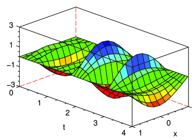
$10v^{\epsilon}$

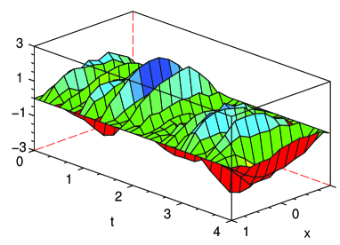
Figure 1: an example realisation of the FitzHugh–Nagumo system (42)–(43) with $\sigma_{1}=0$ , $\sigma_{2}=3$ , $W=(I-A)^{-1}Z$ for a cylindrical Wiener process $Z(t)$, small parameter $\epsilon=0.1$ , and domain $L=1$ .

Consider the following stochastic FitzHugh–Nagumo system with Dirichlet boundary on $[-L,L]$:

$$du^{\epsilon} = \big{[}u_{xx}^{\epsilon}+u^{\epsilon}-(u^{\epsilon})^{3}+v^{\epsilon}\big{]}\,dt\,,$$ (42)

$$dv^{\epsilon} = \frac{1}{\epsilon}\big{[}v_{xx}^{\epsilon}-v^{\epsilon}+u^{\epsilon}\big{]}\,dt+\frac{3}{\sqrt{\epsilon}}\,dW.$$ (43)

$W(t)$ is a $L^{2}(-L,L)$-valued Wiener process with covariance $Q$. Let $A=\partial_{xx}$ with zero Dirichlet boundary on $(-L,L)$ , $f(u,v)=u-u^{3}+v$ , $g(u,v)=-v+u$ , $\sigma_{1}=0$ and $\sigma_{2}=3$ , then (42)–(43) is in the form of (7)–(8). Figure 1 plots an example solution of the FitzHugh–Nagumo system (1)–(2) showing that the noise forcing of $v$ feeds indirectly into the dynamics of $u$.

$|\overline{u^{\epsilon}(0,t)|}$
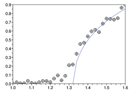
	$L$

Figure 2: rms of the slow mode $u^{\epsilon}(0,t)$ versus the half-length $L$ at parameter $\epsilon=0.1$ for numerical simulations of (42)–(43). This clearly shows the bifurcation that the averaged equation (44) predicts from $L=\pi/2^{5/4}=1.3207$ as shown by the curve.

Furthermore, for any fixed $u$ the spde (43) has a unique stationary solution $\eta_{u}^{\epsilon}$ with distribution

$$\mu_{u}=\mathcal{N}\left((I-\partial_{xx})^{-1}u,\frac{9(I-\partial_{xx})^{-1}Q}{2}+(I-\partial_{xx})^{-2}u\otimes u\right).$$

Then

$$\bar{f}(u)=u-u^{3}+(I-\partial_{xx})^{-1}u\,,$$

and the averaged equation is the deterministic pde

$$du=\big{[}\partial_{xx}u+u-u^{3}+(I-\partial_{xx})^{-1}u\big{]}\,dt\,.$$ (44)

This averaged equation predicts a bifurcation as $L$ increases. For a fundamental mode on $(-L,L)$ of $u=a\cos kx$ for wavenumber $k=\pi/(2L)$, the linear dynamics of the deterministic averaged pde (44) predicts that $u=0$ is stable for $k>2^{1/4}$, that is, $L<\pi/2^{5/4}$. For larger domains with $L>\pi/2^{5/4}=1.3209$ the averaged pde predicts a bifurcation to finite amplitude solutions. This bifurcation matches well with numerical solutions as seen in Figure 2 which plots the mean mid-value as a function of $L$: the bifurcation is clear albeit stochastic.

$100z$

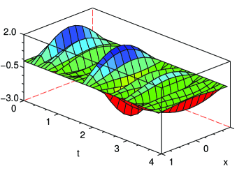
Figure 3: an example realisation of the stochastic deviation (45) for small parameter $\epsilon=0.1$ , $\sigma_{2}=3$ , $Q=(1-\partial_{xx})^{-1}$ and $L=1$.

To quantify the fluctuations evident in the dynamics of $u^{\epsilon}$ we turn to the pde for deviations. Denote by $\eta_{u}$ the unique stationary solution of

$$dv=\big{[}\partial_{xx}v-v+u\big{]}\,dt+dW.$$

Then $f(u,\eta_{u})-\bar{f}(u)=\eta_{u}(t)-(I-\partial_{xx})^{-1}u$ and we have that the deviation $z$ solves the spde

$$dz=\big{[}\partial_{xx}z+(1-3u^{2})z\big{]}\,dt+3(I-\partial_{xx})^{-1}\sqrt{Q}\,d\bar{W}$$ (45)

with $\bar{W}(t)$ being a cylindrical Wiener process defined on a larger probability space with covariance operator $\operatorname{Id}$ on $L^{2}([-L,L])$. Figure 3 plots an example of the deviation between the original system and the averaged system, the spde (45). Including the deviation spde (45) gives a much better approximation than the deterministic averaged equation (44). In particular, when the initial state $u_{0}=0$ and there is no direct forcing of $u$, $\sigma_{1}=0$ , as used in Figures 1 and 3, then the averaged solution is identically $u(t)=0$ . In such a case, the dynamics of $u$ as seen in Figure 1 are modelled solely by deviations governed by the spde (45).

$100\,\text{variance}$
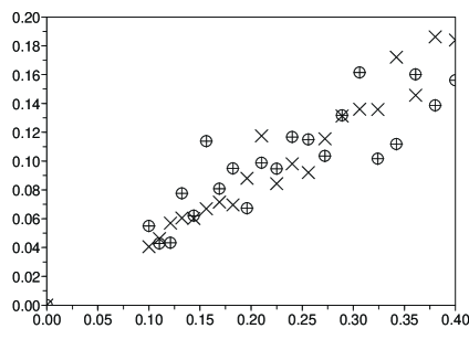
	$\epsilon$

Figure 4: simulations over a time of $128$ (with $L=1$) show: circles, fluctuations in $u^{\epsilon}(0,t)$ whose variance is plotted as function of $\epsilon$ ($\Delta t=0.002$); crosses, fluctuations in $\sqrt{\epsilon}z$ whose variance is plotted as a function of $\epsilon$ ($\Delta t=0.02$). The two agree remarkably well: their standard deviations are best fitted by the nearly identical $0.065\sqrt{\epsilon}$ and $0.066\sqrt{\epsilon}$, respectively.

To quantify the comparison between the deviation pde (45) and the original dynamics of the FitzHugh–Nagumo system (42)–(43), we look at how the fluctuations scale with scale separation parameter $\epsilon$. At $L=1$ the noise free state $u=u^{\epsilon}=0$ is stable. As parameter $\epsilon$ increases the fluctuations in $u^{\epsilon}$ have variance as plotted by circles in Figure 4. The scatter in the plot reflects that averages over much longer times would be better. However, the variance does scale with $\epsilon$ as required, and in close correspondence to that predicted by the deviation pde (45) (crosses).

Acknowledgements

This research was supported by the Australian Research Council grant DP0774311 and NSFC grant 10701072.

References

- [1] V. I. Arnold, V. V. Kozlov & A. I. Neishtadt, Mathematical Aspects of Classical and Celestial Mechanics. Dynamical systems. III. In: Encyclopaedia of Mathematical Sciences, 3rd edn. Springer, Berlin, 2006.
- [2] N. N. Bogolyubov & Y. A. Mitropolskii, Asymptotic Methods in the Theory of Nonlinear Oscillations, Hindustan Publ. Co., 1961.
- [3] S. Cerrai, Second Order PDEs in Finite and Infinite Dimension. A Probabilistic Approach, In: Lecture Notes in Mathematics, Vol. 1762, Springer, Heidelberg, 2001.
- [4] S. Cerrai & M. Freidlin, Averaging principle for a class of stochastic reaction–diffusion equations, Probab. Th. & Rel. Fields, 144(1–2) (2009), 137–177. http://dx.doi.org/10.1007/s00440-008-0144-z
- [5] W. E, X. Li & E. Vanden-Eijnden, Some recent progress in multiscale modeling, Multiscale modelling and simulation, Lect. Notes Comput. Sci. Eng., 39, 3–21, Springer, Berlin, 2004.
- [6] M. I. Freidlin & A. D. Wentzell, Random Perturbations of Dynamical Systems, Second edition, Springer, Heidelberg, 1998.
- [7] H. Kesten & G. C. Papanicolaou, A limit theorem for turbulent diffusion, Commun. Math. Phys., 65(1979), 79–128. http://dx.doi.org/10.1007/3-540-08853-9
- [8] R. Z. Khasminskii, On the principle of averaging the Ito’s stochastic differential equations (Russian), Kibernetika, 4(1968), 260–279.
- [9] Y. Kifer, Diffusion approximation for slow motion in fully coupled averaging, Probab. Th. & Rel. Fields, 129 (2004), 157–181. http://dx.doi.org/10.1007/s00440-003-0326-7
- [10] P. Imkeller & A. Monahan (Eds.). Stochastic Climate Dynamics, a Special Issue in the journal Stoch. and Dyna., 2(3), 2002.
- [11] M. Metivier, Stochastic Partial Differential Equations in Infinite Dimensional Spaces, Scuola Normale Superiore, Pisa, 1988.
- [12] G. Da Prato & J. Zabczyk, Stochastic Equations in Infinite Dimensions, Cambridge University Press, 1992.
- [13] J. Simon, Compact sets in the space , Ann. Mat. Pura Appl., 146 (1987), 65–96. http://dx.doi.org/10.1007/BF01762360
- [14] R. Temam & A. Miranville, Mathematical Modeling in Continuum Mechanics, Second edition, Cambridge University Press, Cambridge, 2005.
- [15] V. M. Volosov, Averaging in systems of ordinary differential equations. Russ. Math. Surv., 17(1962), 1–126. http://dx.doi.org/10.1070/RM1962v017n06ABEH001130
- [16] H. Watanabe, Averaging and fluctuations for parabolic equations with rapidly oscillating random coefficients, Probab. Th. & Rel. Fields, 77 (1988), 359–378. http://dx.doi.org/10.1007/BF00319294
- [17] E. Waymire & J. Duan (Eds.), Probability and Partial Differential Equations in Modern Applied Mathematics. IMA Volume 140, Springer–Verlag, New York, 2005.