An Atlas of Predicted Exotic Gravitational Lenses

Abstract

Wide-field optical imaging surveys will contain tens of thousands of new strong gravitational lenses. Some of these will have new and unusual image configurations, and so will enable new applications: for example, systems with high image multiplicity will allow more detailed study of galaxy and group mass distributions, while high magnification is needed to super-resolve the faintest objects in the high redshift universe. Inspired by a set of six unusual lens systems [including five selected from the Sloan Lens ACS (SLACS) and Strong Lensing Legacy (SL2S) surveys, plus the cluster Abell 1703], we consider several types of multi-component, physically-motivated lens potentials, and use the ray-tracing code glamroc to predict exotic image configurations. We also investigate the effects of galaxy source profile and size, and use realistic sources to predict observable magnifications and estimate very approximate relative cross-sections. We find that lens galaxies with misaligned disks and bulges produce swallowtail and butterfly catastrophes, observable as “broken” Einstein rings. Binary or merging galaxies show elliptic umbilic catastrophes, leading to an unusual Y-shaped configuration of 4 merging images. While not the maximum magnification configuration possible, it offers the possibility of mapping the local small-scale mass distribution. We estimate the approximate abundance of each of these exotic galaxy-scale lenses to be $\sim 1$ per all-sky survey. In higher mass systems, a wide range of caustic structures are expected, as already seen in many cluster lens systems. We interpret the central ring and its counter-image in Abell 1703 as a “hyperbolic umbilic” configuration, with total magnification $\sim 100$ (depending on source size). The abundance of such configurations is also estimated to be $\sim 1$ per all-sky survey.

1 Introduction

Strong gravitational lenses, by producing multiple images and high magnification, can teach us much about galaxies, how they form and how they evolve. The numerous constraints allow us to determine the mass distribution of galaxies, groups and clusters, including invisible dark substructure. On the other hand, strong lens systems, by the high magnification they provide, can act as cosmic telescopes, leading to far more observed flux and thereby opening unique windows into the early universe.

Until recently, apart from a very few exceptions (e.g. Rusin et al., 2001), the lens configurations observed have been Einstein ring, double and quadruple image configurations. As the number of discovered lenses increases, these configurations will become commonplace and truly exotic ones should come into view. Indeed, several recent strong lens surveys have proved to be just big enough to contain the first samples of complex galaxy-scale and group-scale strong lenses capable of producing exotic high magnification image patterns. One such survey is the Sloan Lens ACS survey (SLACS, Bolton et al., 2006, 2008), which uses the SDSS spectroscopic survey to identify alignments of relatively nearby massive elliptical galaxies with star-forming galaxies lying behind them, and then the Advanced Camera for Surveys (ACS) onboard the Hubble Space Telescope (HST) to provide a high resolution image to confirm that multiple-imaging is taking place. Another is the Strong Lens Legacy Survey (SL2S, Cabanac et al., 2007), which uses the 125-square degree, multi-filter CFHT Legacy Survey images to find rings and arcs by their colors and morphology. Together, these surveys have discovered more than 100 new gravitational lenses.

Moreover, strong lensing science is about to enter an exciting new phase: very wide field imaging surveys are planned for the next decade that will contain thousands of new lenses for us to study and exploit. For example, the Large Synoptic Survey Telescope (LSST, Ivezic et al., 2008) will provide deep ($\approx 27$th AB magnitude), high cadence imaging of 20,000 square degrees of the Southern sky in 6 optical filters, with median seeing $0.7$ arcseconds. Similarly, the JDEM and Euclid (Laureijs et al., 2008) space observatories are planned to image a similar amount of sky at higher resolution (0.1–0.2 arcseconds), extending the wavelength coverage into the near infra-red (the SNAP design, Aldering et al. 2004, with its weak lensing-optimised small pixels and large field of view, would be particularly effective at finding strong lenses in very large numbers). With such panoramic surveys on the drawing board, we may begin to consider objects that occur with number densities on the sky of order $10^{-4}$ per square degree or greater.

In order to understand the contents of these forthcoming surveys, it is useful to have an overview of the configurations, magnifications and abundances we can expect from exotic gravitational lenses, namely those with complex mass distributions and fortuitously-placed sources. Several attempts have already been made in this direction, generally focusing on individual cases. This field of research is centred on the notion of critical points (“higher-order catastrophes” and “calamities”) in the 3-dimensional space behind a massive object. These points are notable for the transition in image multiplicity that takes place there, and have been studied in a number of different situations by various authors in previous, rather theoretical works (e.g. Blandford & Narayan, 1986; Kassiola et al., 1992; Kormann et al., 1994; Keeton et al., 2000; Evans & Witt, 2001).

Here, we aim to build on this research to provide an atlas to illustrate the most likely observable exotic lenses. Anticipating the rarity of exotic lenses, we focus on the most readily available sources, the faint blue galaxies (e.g. Ellis, 1997), and investigate the effect of their light profile and size on the images produced. Our intention is to improve our intuition of the factors that lead to exotic image configurations. What are the magnifications we can reach? Can we make a first attempt at estimating the abundances of lenses showing higher-order catastrophes? Throughout this paper, we emphasize the critical points associated with plausible physical models, and try to remain in close contact with the observations.

To this end, we select six complex lenses (three from the SLACS survey, two from the SL2S survey, and the galaxy cluster Abell 1703 from Limousin et al. 2008b) to motivate and inspire an atlas of exotic gravitational lenses. By making qualitative models of these systems we identify points in space where, if a source were placed there, an exotic lens configuration would appear. We then extend our analysis to explore the space of lens model parameters: for those systems showing interesting caustic structure, that is to say presenting higher-order catastrophes, we study the magnifications we can reach, and make very rough estimates of the cross-sections and abundances of such lenses.

This paper is organised as follows. In Section 2 we provide a review of the basic theory of gravitational lenses and their singularities, and then describe in Section 3 our methodology for estimating the source-dependent magnifications and cross-sections of gravitational lenses. We then present, in Section 4, our sample of unusual lenses, explaining why we find them interesting. Suitably inspired, we then move on the atlas itself, focusing first on simple, i.e. galaxy-scale, lens models (Section 5), and then on more complex, i.e. group-scale and cluster-scale lenses (Section 6). Finally, we use the cross-sections calculated in Sections 5 and 6 to make the first (albeit crude) estimates of the abundance of exotic lenses for the particular cases inspired by our targets in Section 7. We present our conclusions in Section 8. When calculating distances we assume a general-relativistic Friedmann-Robertson-Walker (FRW) cosmology with matter-density parameter $\Omega_{m}=0.3$, vacuum energy-density parameter $\Omega_{\Lambda}=0.7$, and Hubble parameter $H_{0}=70$ km s^-1 Mpc^-1.

2 Gravitational lensing theory

This section is divided into two parts. We first briefly review the relevant basic equations in lensing theory, following the notation of Schneider et al. (2006). We then introduce the qualitative elements of lens singularity theory (Petters et al., 2001) relevant to this study.

2.1 Basics

We reproduce in Fig. 1 a sketch, from Schneider et al. (2006), of a typical gravitational lens system. In short, a lens system is a mass concentration at redshift $z_{\rm d}$ deflecting the light rays from a source at redshift $z_{\rm s}$. The source and lens planes are defined as planes perpendicular to the optical axis.

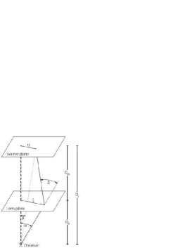
Figure 1: Schema of a typical, single plane, gravitational lens system – from Schneider et al. (2006, Figure 12, p. 20, reproduced with permission ©ESO).

The lens equation relates the position of the source to its observed position on the sky; in the notation of the sketch, $\boldsymbol{\beta}=\boldsymbol{\theta}-\boldsymbol{\alpha}(\boldsymbol{\theta})$ where $\boldsymbol{\beta}=(\beta_{1},\beta_{2})$ denotes the angular position of the source, $\boldsymbol{\theta}=(\theta_{1},\theta_{2})$ the angular position of the image and $\boldsymbol{\alpha}(\boldsymbol{\theta})=\frac{D_{\rm ds}}{D_{\rm s}}\boldsymbol{\hat{\alpha}}(D_{\rm d}\boldsymbol{\theta})$ is the scaled deflection angle. $D_{\rm d}$, $D_{\rm s}$, and $D_{\rm ds}$ are the angular diameter distances to the lens, to the source, and between the lens and the source respectively.

The dimensionless surface mass density or convergence is defined as

$$\kappa(\boldsymbol{\theta})\equiv\dfrac{\Sigma(D_{\rm d}\boldsymbol{\theta})}{\Sigma_{\rm crit}}\quad\text{with}\quad\Sigma_{\rm crit}\equiv\dfrac{c^{2}}{4\pi G}\dfrac{D_{\rm s}}{D_{\rm d}D_{ds}}$$ (1)

where the critical surface mass density $\Sigma_{\rm crit}$ delimits the region producing multiple images (within which $\langle\kappa\rangle\geq 1$). The critical surface mass density is, therefore, a characteristic value for the surface mass density which is the dividing line between “weak” and “strong” lenses (Schneider et al., 2006, p. 21).

Gravitational lensing conserves surface brightness, but the shape and size of the images differs from those of the source. The distortion of the images is described by the Jacobian matrix,

$${\bf J}(\boldsymbol{\theta}) =\dfrac{\partial\boldsymbol{\beta}}{\partial\boldsymbol{\theta}}=\left(\delta_{ij}-\dfrac{\partial^{2}\psi(\boldsymbol{\theta}}{\partial\theta_{i}\partial\theta_{j}}\right)$$ (2)

$$=\left(\begin{array}[]{cc}1-\kappa-\gamma_{1}&-\gamma_{2}\\ -\gamma_{2}&1-\kappa+\gamma_{1}\end{array}\right),$$ (5)

where we have introduced the components of the shear $\gamma\equiv\gamma_{1}+i\gamma_{2}$. Both the shear and the convergence can be written as combinations of partial second derivatives of a lensing potential $\psi$:

$$\kappa = \dfrac{1}{2}(\psi_{,11}+\psi_{,22}),$$ (6)

$$\gamma_{1} = \dfrac{1}{2}(\psi_{,11}-\psi_{,22}),\quad\gamma_{2}=\psi_{,12}.$$ (7)

The inverse of the Jacobian, ${\bf M}(\boldsymbol{\theta})={\bf J}^{-1}$, is called the magnification matrix, and the magnification at a point $\boldsymbol{\theta_{0}}$ within the image is $|\mu(\boldsymbol{\theta_{0}})|$, where $\mu=\mathrm{det}~{}{\bf M}$.

The total magnification of a point source at position $bs{\beta}$ is given by the sum of the magnifications over all its images,

$$\mu_{\rm p}(\boldsymbol{\beta})=\sum_{i}|\mu(\boldsymbol{\theta_{i}})|,$$ (8)

The magnification of real sources with finite extent is given by the weighted mean of $\mu_{\rm p}$ over the source area,

$$\mu=\dfrac{\int d^{2}\beta~{}I^{(s)}(\boldsymbol{\beta})\mu_{\rm p}(\boldsymbol{\beta})}{\left[\int d^{2}\beta~{}I^{(s)}(\boldsymbol{\beta})\right]},$$ (9)

where $I^{(s)}(\boldsymbol{\beta})$ is the surface brightness profile of the source.

2.2 Singularity theory and caustic metamorphoses in gravitational lensing

The critical curves are the smooth locii in the image plane on which the Jacobian vanishes and the point magnification is formally infinite. The caustics are the corresponding curves, not necessarily smooth, obtained by mapping the critical curves into the source plane via the lens equation.

A typical caustic presents cusp points connected by fold lines, which are the generic singularities associated with strong lenses (Kassiola et al. (1992)). By this we mean that these two are stable in the source plane, i.e. the fold and cusp are present in strong lenses for all $z_{\rm s}>z_{\rm d}$. By considering a continuous range of source-planes, the folds can be thought of as surfaces in three-dimensional space extending behind the lens, while cusps are ridgelines on these surfaces. Indeed, this is true of all caustics: they are best thought of as three-dimensional structures (surfaces) lying behind the lens, which are sliced at a given source redshift and hence renderable as lines on a 2-dimensional plot. We will show representations of such three-dimensional caustics later. Other singularities can exist but they are not stable, in the sense that they form at a specific source redshift, or in a narrow range of source redshifts: they represent single points in three-dimensional space. The unstable nature of these point-like singularities can be used to put strong constraints on lens models and can lead to high magnifications (Bagla, 2001) – it is these exotic lenses that are the subject of this paper.

Excellent introductions to gravitational lenses and their critical points can be found in the books by Schneider et al. (1992, where chapter 6 is particularly relevant) and Petters et al. (2001); here we provide a brief overview. We will consider at various points the following critical points (known as “calamities” or “catastrophes”): lips, beak-to-beak, swallowtail, elliptic umbilic and hyperbolic umbilic. With these singularities, we associate metamorphoses: the beak-to-beak and lips calamities, and the swallowtail catastrophe, mark the transition (as the source redshift varies) from zero to two cusps, the elliptic umbilic catastrophe from three to three cusps, and the hyperbolic umbilic catastrophe involves the exchange of a cusp between two caustic lines (Schneider et al., 1992, section 6.3). These are the five types of caustic metamorphosis that arise generically from taking planar slices of a caustic surface in three dimensions. As well as these, we will study the butterfly metamorphosis, which involves a transition from one to three cusps. It can be constructed from combinations of swallowtail metamorphoses; lenses that show butterfly metamorphoses will have high image multiplicities, hence our consideration of them as “exotic” systems. Petters et al. (2001, section 9.5) give an extensive discussion of these caustic metamorphoses, and we encourage the reader to take advantage of this.

In Fig. 2 and Fig. 3, which are reproduced and extended from Petters et al. (2001), we sketch these critical points and their related metamorphoses, showing the changes in image multiplicity $N$ at the transition. The features in the caustics after the swallowtail and butterfly metamorphoses are also referred to as, respectively, swallowtails and butterflies after their respective shapes. A caustic shrinking to an elliptic umbilic catastrophe and then appearing again is called a “deltoid” caustic (Suyu & Blandford, 2006). We note that varying source redshift is not the only way to bring about a metamorphosis: the independent variable could also be the lens component separation in a binary lens, the isopotential ellipticity, the density profile slope and so on. In this paper we aim to illustrate these metamorphoses in plausible physical situations.

A number of theoretical studies of these critical points have already been performed. Blandford & Narayan (1986) undertook the first major study of complex gravitational lens caustics, and provided a classification of gravitational lens images. Following this initial foray, Kassiola et al. (1992) studied the lips and beak-to-beak “calamities,” applied to the long straight arc in Abell 2390. Kormann et al. (1994) presented an analytical treatment of several isothermal elliptical gravitational lens models, including the singular isothermal ellipsoid (SIE) and the non-singular isothermal ellipsoid (NIE). Keeton et al. (2000) focused on the most common strong lenses, namely isothermal elliptical density galaxies in the presence of tidal perturbations. Evans & Witt (2001) presented, via the use of boxiness and skewness in the lens isopotentials, the formation of swallowtail and butterfly catastrophes, while most recently Shin & Evans (2008b) treated the case of binary galaxies case, outlining in particular the formation of the elliptic umbilic catastrophe.

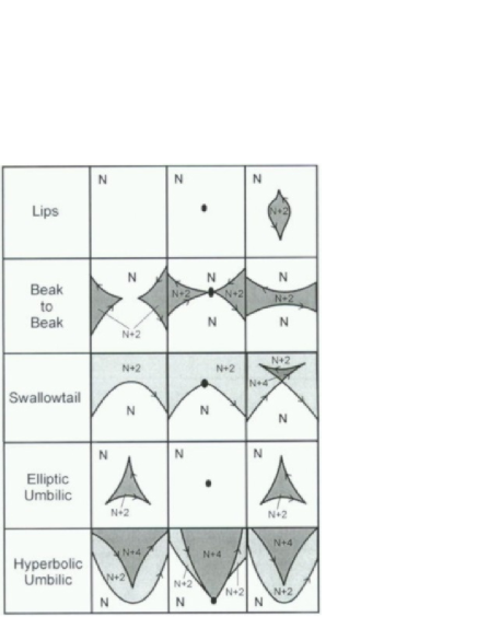
Figure 2: Caustic metamorphoses and their lensed image multiplicities. The points determine the critical points. The numbers $N$, $N+2$, $N+4$ indicate how many lensed images are produced of a light source lying in the given region. The caustic curves are oriented so such that, locally, light sources to the left generically have two more lensed images than those to the right. Adapted from Figure 9.19 in Petters et al. (2001, p. 382). With kind permission of Springer Science$+$Business Media.

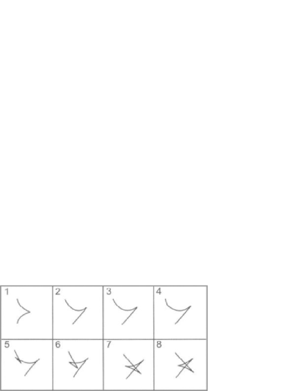
Figure 3: A butterfly caustic metamorphosis, including a swallowtail as an intermediate step. Adapted from Figure 9.17 in Petters et al. (2001, p. 379). With kind permission of Springer Science$+$Business Media.

The mathematical definitions of the various catastrophes (given in chapter 9 of Petters et al., 2001, and the above papers, along with some criteria for these to occur), involve various spatial derivatives of the Jacobian, as well as the magnification itself. This is the significance of the “higher-order” nature of the catastrophes: they are points where the lens potential and its derivatives are very specifically constrained. This fact provides strong motivation for their study – lenses showing image configurations characteristic of higher-order catastrophes should allow detailed mapping of the lens local mass distribution to the images. In addition, the large changes in image multiplicity indicate that these catastrophe points are potentially associated with very high image magnifications, perhaps making such lenses very useful as cosmic telescopes.

3 Source sizes and observable magnification

We are interested in the most likely instances of exotic lensing by systems close to catastrophe points. The most common strong lenses are galaxies lensed by galaxies, and so it is on these systems that we focus our attention. The observability of strong lensing depends quite strongly on the magnification induced – and this in turn depends on the source size, as indicated in Equation 9. In this section we investigate this effect.

We compute maps of the total magnification in the source plane, $\mu_{\rm p}(\boldsymbol{\beta})$ in Equation 8, using the ray-tracing code glamroc (described in the appendix). In order to study the magnification of realistic extended sources, we convolve these magnification maps by images of plausible sources, described by elliptically symmetric surface brightness distributions with Sersic – Gaussian, exponential or de Vaucouleurs – profiles (see the appendix for more details). We then use these to quantify how likely a given magnification is to appear by calculating: a) the fraction of the multiply-imaged source plane area that has magnification above some threshold, and conversely b) the magnification at a given fractional cross-sectional area.

We first use these tools to analyze the likely effect of source size and profile on the observable magnification. We consider a standard lens model, with a non-singular isothermal profile (see appendix), and a fiducial source at redshift $z_{\rm s}=2$ with half-light radius $2.9$kpc (Ferguson et al., 2004). The lens model and four magnification maps are presented in Fig. 4. In Fig. 5 we then plot the corresponding fractional cross-section area as a function of threshold total magnification. We first remark that the area of multiple imaging corresponds approximately to the area with magnification greater than 3, a value we will take as a point of reference in later sections. The behaviour of the three source profiles is fairly similar, with the peakier profiles giving rise to slightly higher probabilities of achieving high magnifications. The two profiles we expect to be more representative of faint blue galaxies at high redshift, the exponential and Gaussian, differ in their fractional cross-sectional areas by less than $10\%$.

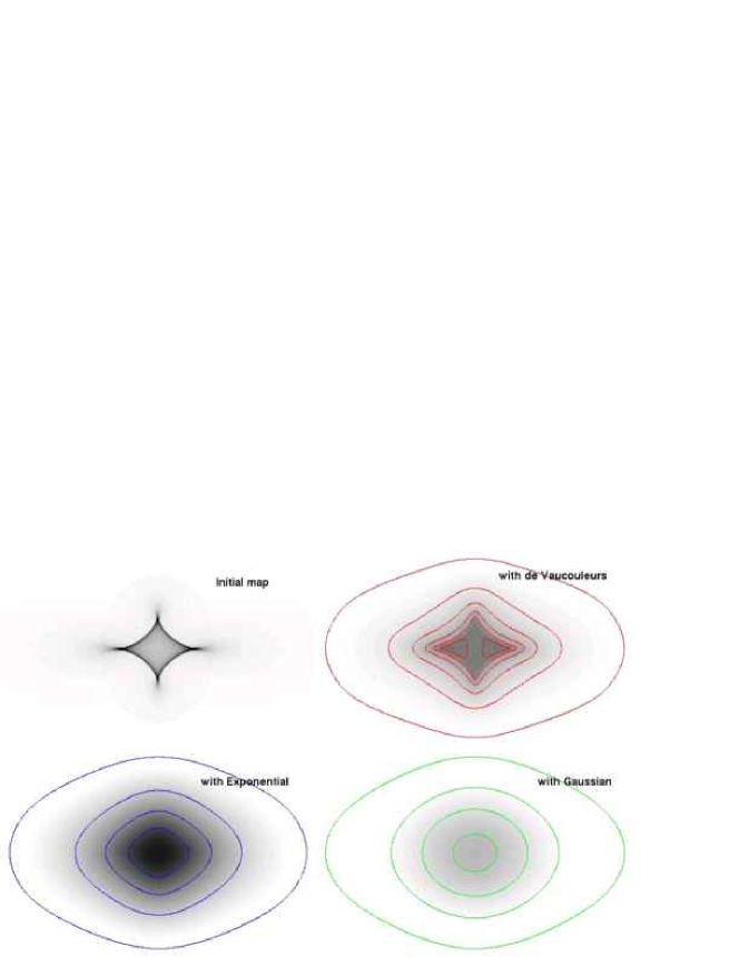
Figure 4: Upper panel: critical curves (left) and caustics (right) of an elliptically-symmetric galaxy modelled by an NIE profile (appendix). The source can be seen lying close to a cusp, giving three merging images, a fainter counter-image and a de-magnified central image. Lower panel: source-plane total magnification maps convolved with four different source types: point source, de Vaucouleurs bulge, exponential disk, Gaussian. Contours of equal magnification are shown on all three convolved maps, overlaid on the arbitrary greyscale images: note the higher magnifications reached with the peakiest de Vaucouleurs profile.

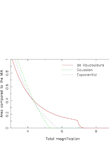
Figure 5: The fractional cross-sectional area (relative to the multiple imaging area) as a function of threshold total magnification, for a model NIE galaxy. The source half-light radius was fixed at 2.9kpc.

We now turn to influence of the half-light radius on the observable magnification, considering only the exponential profile and keeping the fiducial source redshift of $z_{\rm s}=2$. We plot two graphs in Fig. 6: both as a function of half-light radius $r_{\rm e}$, we show the fractional cross-sectional area greater than some magnification threshold, and also the magnification corresponding to a given fractional area threshold. We study an inclusive range of half light-radii, from 0.5 kpc to 5 kpc (Marshall et al. (2007) give an example of a compact source of half-light radius $\simeq$0.6 kpc).

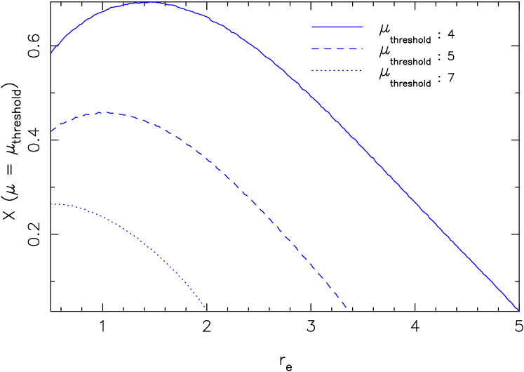
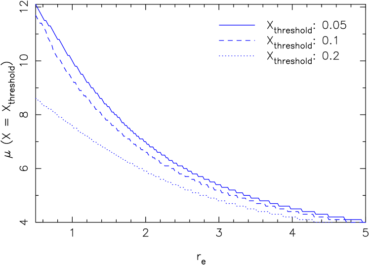
Figure 6: Upper panel: for an exponential profile source, we plot the fractional cross-sectional area for magnifications greater than various magnification thresholds, as a function of the half-light radius $r_{\rm e}$ (in kpc, $z_{\rm s}=$). Lower panel: the corresponding magnification for a given fractional cross-sectional area threshold, also as a function of $r_{\rm e}$.

We see that the magnification is, indeed, highly dependent on the source size: the smaller the source, the more likely a large total magnification is (lower panel). At small magnification, the fractional cross-sectional area reaches a maximum: larger sources smear out the magnification map more, while smaller sources have already resolved the magnification map at that threshold and cannot increase the interesting area.

Clearly the size of the source is more important than the form of the source profile. Henceforth we use only one profile, the exponential, and study three different sizes: 0.5 kpc, 1.5 kpc and 2.5 kpc, keeping these constant in redshift for simplicity in the analysis. At low redshift, these sizes are somewhat smaller than the ones discussed in Ferguson et al. (2004) (and the appendix). One might argue that such an arbitrary choice is not unreasonable, given the uncertainty and scatter in galaxy sizes at high redshift. The magnification bias noted here will play some role in determining the abundance of lensing events we observe; however, as we discuss later, we leave this aspect to further work. In this paper we simply illustrate the effects of source size on the observability of various lensing effects, noting that 0.5–2.5 kpc represents a range of plausible source sizes at $zs\gtrsim 1$.

4 A sample of unusual lenses

The majority of the known lenses show double, quad and Einstein ring image configurations well reproduced by simple SIE models. There are several cases of more complex image configurations due to the presence of several sources; there are also a few more complex, multi-component lens systems, leading to more complex caustic structures. One example of such a complex and interesting lens is the B1359$+$154 system, composed of 3 lens galaxies giving rise to 6 images Rusin et al. (2001). Another example is MG2016$+$112, whose quasar images have flux and astrometric anomalies attributable to a small satellite companion (Mor++09, and references therein).

We here show here six unusual lenses that have either been recently discovered or studied: three from the SLACS survey (Bolton et al., 2008), two from the SL2S survey (Cabanac et al., 2007), and the rich cluster Abell 1703 (Limousin et al., 2008b). This set presents a wide range of complexity of lens structure. These lenses are presented in this section but are not subject of further studies in the following sections: their function is to illustrate the kinds of complex mass structure that can arise in strong lens samples given a large enough imaging survey. All six have extended galaxy sources, as expected for the majority of strong lenses detected in optical image survey data.

The three SLACS targets are massive galaxies at low redshift ($z_{\rm d}\sim 0.2$), that are not as regular as the majority of the SLACS sample (Bolton et al., 2008), instead showing additional mass components such as a disk as well as a bulge, or a nearby satellite galaxy. The two SL2S targets are more complex still, being compact groups of galaxies. The presence of several lensing objects makes them rather interesting to study and a good starting points for our atlas. The cluster Abell 1703 was first identified as a strong lens in the SDSS imaging data by Hennawi et al. (2008), and was recently studied with HST by Limousin et al. (2008b). As we will see, elliptical clusters such as this can give rise to a particular higher-order catastrophe, the hyperbolic umbilic.

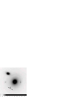
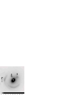
Figure 7: Three unusual SLACS lenses. HST/ACS images in the F814W filter, approximately 6 arcsec on a side. Left: SDSSJ1100$+$5329; centre: SDSSJ0808$+$4706; right: SDSSJ0956$+$5100. In this final image, we denote: 1) the main lens galaxy; 2) the satellite lens galaxy; 3) the counter-image to the extended arc system.

4.1 The three SLACS lenses

Three unusual SLACS lenses are presented in Fig. 7. SDSSJ1100$+$5329 presents a large circular arc relatively far from the lens ($\sim 1.5$”), broken at its centre. We were able to model this system with two SIE profiles of different ellipticities but with the same orientations, representing a mass distribution comprising both a bulge and a disk. While a detailed modeling will be presented elsewhere, we take a cue from SDSSJ1100$+$5329 and study in Section 5 the catastrophe points present behind disk-plus-bulge lenses.

SDSSJ0808$+$4706 is a massive elliptical galaxy with a large satellite galaxy lying just outside the Einstein ring and distorting its shape. SDSSJ0956$+$5100 also has a satellite galaxy, this time inside the Einstein radius (the arcs due to the lensing effect are at larger radius than the satellite). The image component labeled 3 in Fig. 7, is considered to be due to the lensing effect: the system of images to which it belongs is clearly distorted by the satellite. Inspired by these two systems, we study below the catastrophes lying behind binary lenses, a subject also investigated by Shin & Evans (2008a).

4.2 The two SL2S lenses

We consider two lenses from the SL2S survey (Cabanac et al., 2007): SL2SJ0859$-$0345 and SL2SJ1405$+$5502. In SL2SJ1405$+$5502 we have an interesting binary system leading to an asymmetric “Einstein Cross” quad configuration (Figure 8). Binary systems, as we will see in Section 6 below can develop exotic caustic structures (as discussed by Shin & Evans (2008a)). We are able to reproduce the image configuration fairly well with a simple binary lens model, and present its critical curves and caustics in Section 6 below.

SL2SJ0859$-$0345 is more complex, consisting of 4 or 5 lens components in a compact group of galaxies (Limousin et al., 2008a). The image configuration is very interesting: an oval-shaped system of arcs, with 6 surface brightness peaks visible in the high resolution (low signal-to-noise) HST/WFPC2 (Wide-Field and Planetary Camera 2) image. It is in this single-filter image that the fifth and faintest putative lens galaxy is visible; it is not clear whether this is to be considered as a lens galaxy, or a faint central image. In Fig. 9 we show the WFPC2 and CFHTLS images, and in the central panel a version of the latter with the four brightest lens components modelled with galfit (in each filter independently) and subtracted. The central faint component remains undetected following this process, due to its position between the sidelobes of the fit residuals. We will improve this modelling elsewhere; here, in Section 6, we simply investigate a qualitatively successful 4-lens galaxy model of the system, focusing again on the exotic critical curve and caustic structures and the critical points therein.

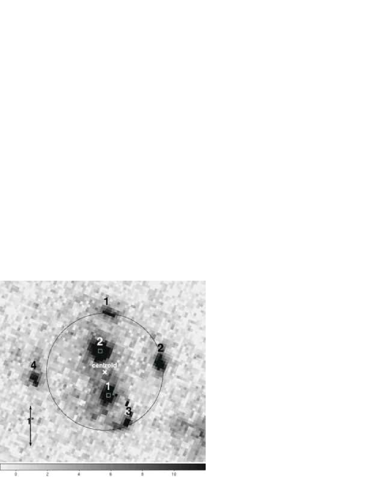
Figure 8: SJ1405+5502, found in the CFHTLS data (top, g-r-i composite) and followed-up with HST/WFPC2 in Snapshot mode with the F606W filter (bottom). Both images are approximately 6 arcsec on a side

Figure 9: The complex lens system SL2SJ0859$-$0345. Left: g-r composite image from CFHTLS; centre: after subtraction of the four bright lens components; right: at higher resolution, with HST/WFPC2 in the F606W filter. Images are approximately 15 arcsec on a side.

4.3 Abell 1703

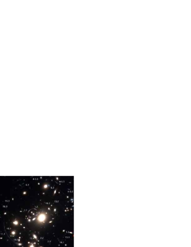
Figure 10: Central part of the cluster Abell 1703, imaged with HST/ACS and reproduced from Limousin et al. (2008b). We are interested in the bright central ring (images 1.1–1.4), and its counter-image (1.5).

The strong lensing galaxy cluster Abell 1703 ($z_{\rm d}=0.28$, shown in Fig. 10, reproduced from Limousin et al. 2008b) exhibits an interesting feature: a central ring with a counter-image. A naive interpretation would link this central-quad feature to the two small galaxies lying inside it; however, the large image separation across the quad and the presence of the spectroscopically-confirmed counter-image argue against this. We instead interpret the image configuration as being due to a source lying close to a hyperbolic umbilic catastrophe, a critical point anticipated for elliptically-extended clusters such as this one (Kassiola et al., 1992).

5 Simple lens models

Motivated by our SLACS targets, we study in this section two different “simple” lens models: a single galaxy composed of both a bulge and a disk, and a main galaxy with a companion satellite galaxy. In this respect the adjective “simple” could also be read as “galaxy-scale.” We will investigate some “complex,” group-scale lens models in the next section.

Aa single isothermal elliptical galaxy yields at most four visible images; higher multiplicities can be obtained when considering deviations from such profiles, leading to more than four images, as shown by e.g. (Keeton et al., 2000). Likewise, (Evans & Witt, 2001) showed how boxy or disky lens isodensity contours can give rise to six to seven image systems. Here we construct models from sums of mass components to achieve the same effect, associated with the swallowtail and butterfly metamorphoses.

5.1 Galaxies with both bulge and disk components

5.1.1 Model

We model a galaxy with both a disc and a bulge using two concentric NIE models with small core radii, different masses and different ellipticities. These two NIE components are to be understood as a bulge-plus-halo and a disk-plus-halo components, as suggested by the “conspiratorial” results of the SLACS survey (Koopmans et al., 2006). For brevity we refer to them as simply the bulge and disk components.

We fix the total mass of the galaxy to be that of a fiducial massive early-type galaxy, with overall velocity dispersion of $\sigma=250$km s^-1, and impose the lens Einstein radius to correspond to this value of $\sigma$. We then divide the mass as $\sigma_{\rm bulge}=200$ and $\sigma_{\rm disk}=150$km s^-1 to give a bulge-dominated galaxy with prominent disk, such as that seen in SDSSJ1100$+$5329. Integrating the convergence, we calculate the ratio of the mass of the bulge component to the total mass, and find $f=\frac{M_{\rm E,bulge}}{M_{\rm E,total}}=0.64$, where $M_{\rm E}$ indicates the mass enclosed within the Einstein radius. This ratio is somewhat low for a lens galaxy, but not extremely so: Möller et al. (2003) studied a theoretical population of disky lenses, and found that around one quarter of their sample had bulge mass fraction less than this.

The parameters of our double NIE model are summarised as follows:

Type	$\sigma$	$\epsilon^{\prime}$	$r_{\rm c}$	$\phi$
Bulge	200	0.543	0.1	0.0
Disk	150	0.8	0.1	$\phi$

Here the variable $\phi$ represents the relative orientation of the two components’ major axes, and $\sigma$ is measured in km s^-1, $r_{\rm c}$ in kpc, $\theta$ in arcseconds and $\phi$ in radians. The ellipticity $\epsilon^{\prime}$ refers to the mass distribution (see the appendix for more details). Predicted lens system appearances, and critical and caustic curves, are shown in Fig. 11, for three values of the misalignment angle $\phi$.

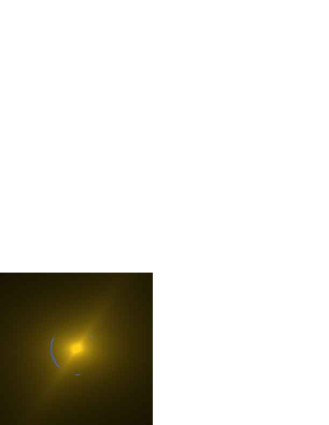
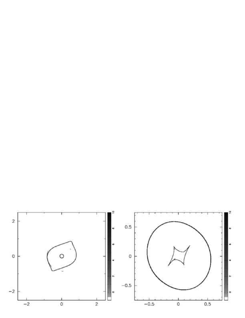
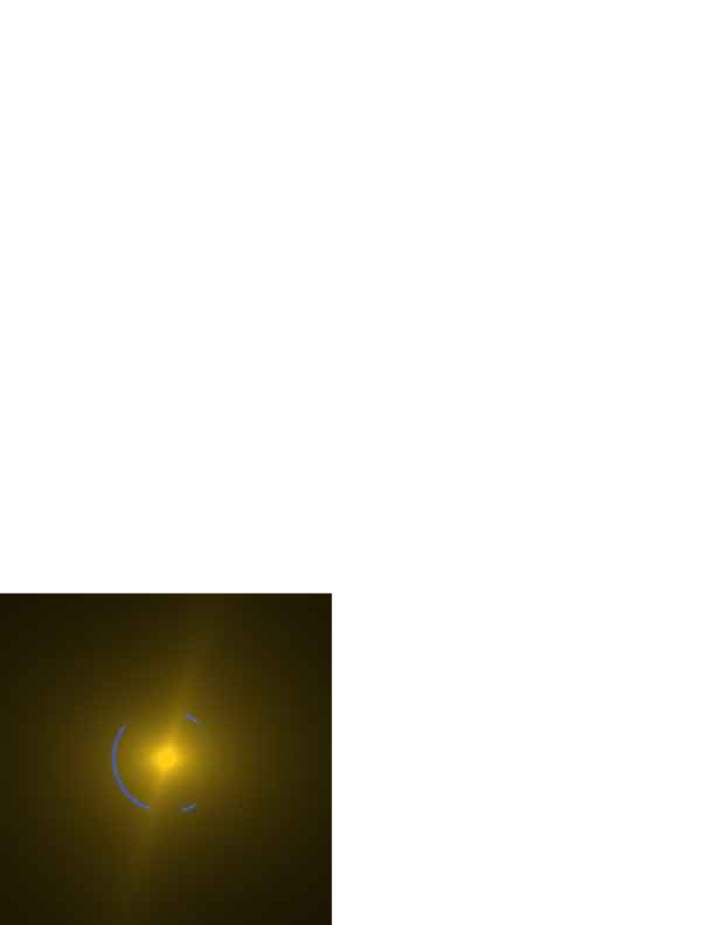
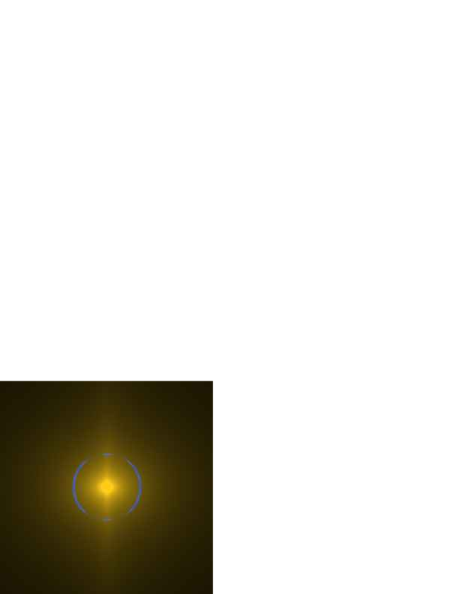
Figure 11: Gravitational lensing due to a model bulge-dominated, disky galaxy. Three different bulge-disk misalignment angles $\phi$ are shown: from top to bottom, $\phi=1.0,~{}1.3,~{}1.57$ radians. Left to right: a predicted high-resolution optical image; the critical curves and image positions (note the small inner critical curve arising from the presence of the small core radius in the NIE profile); the source position relative to the caustics. For the anti-aligned case, $\phi=1.57$, two butterflies overlap in the centre of the source-plane giving rise to an Einstein ring image system composed of 8 merging images, visible here for the case of an almost point-like source.

5.1.2 Critical curves, caustics and image configurations

The mapping of the outer critical curve to the source plane (right panels of Fig. 11) gives quite complex caustic curves, depending of the orientation. For $\phi=0$, the profile is quasi-elliptical, and the inner caustic is a familiar astroid shape. As $\phi$ increases, the astroid caustic becomes skewed. At $\phi\simeq 1$, two of the folds “break” in to two swallowtail catastrophes (at opposing points). This critical value of $\phi$ varies with disk-to-bulge ratio, and the ellipticities of the two components: larger ellipticities or disk-to-bulge ratios give more pronounced asymmetry, and a smaller $\phi$ is required to break the folds. For $\phi>\phi_{\rm crit}$, we observe two swallowtails presenting two additional cusps each. As $\phi$ approaches $\pi/2$, each swallowtail migrates to a cusp, and produces a butterfly (we can also obtain two butterflies with $\phi<\pi/2$, if we increase the asymmetry). If the asymmetry is sufficiently large, the two butterflies overlap, producing a nine-imaging region (eight visible images and a de-magnified central image). In the same way, two swallowtails can overlap, producing also a seven-imaging region (six images in practice). Evans & Witt (2001) and Keeton et al. (2000) give analytical solutions to produce such regions by using, respectively, deviations of isophotes (boxiness and skew) and by adding external shear corresponding to external perturbations. All we show here is that the combination of realistic disk and bulge mass components is a physical way to obtain such distorted isodensity contours; the disk-to-bulge ratio and their misalignment can be straightforwardly estimated using standard galaxy morphology tools.

Observationally speaking, it is important to note that the various critical areas (the swallowtail and butterfly, and the regions of overlap between them) are very small, and close to the optical axis of the lens. A small source lying in one of these regions will appear either as a very large arc (four images merging in the case of a swallowtail, five images merging in the case of a butterfly), or as a “broken” Einstein ring (in the nine-imaging region cases). However, in practice, with realistic source sizes, these image configurations will appear as Einstein rings, around which the surface brightness varies: this is illustrated in Fig. 12, where we predict optical images for the same lens models as in Fig. 11 but with a source at $z_{\rm s}=1.2$ with $r_{\rm e}=2$ kpc. These fluctuations can tell us something about the detailed structure of the large-scale potential, and should be borne in mind when modelling such rings (Koopmans, 2005; Vegetti & Koopmans, 2009).

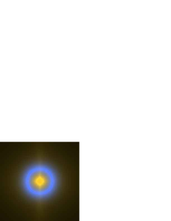
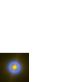
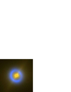
Figure 12: Gravitational lensing due to a model bulge-dominated, disky galaxy, and a realistic faint blue galaxy source. The same three bulge-disk misalignment angles $\phi$ as in Fig. 11 are shown: $\phi=1.0,~{}1.3,~{}1.57$ radians, from left to right. The source is at $z_{s}=1.2$ and has a half-light radius of 2 kpc.

5.1.3 Magnification

In order to study the magnification of this model system, we first plot in Fig. 13the fractional cross-sectional area as a function of the magnification for the almost maximally-misaligned case, $\phi=1.55$. We show three different source sizes (as in Section 3). For a typical extended source ($r_{\rm e}=$ 2.5 kpc), the total magnification only reaches a maximum of around $\mu=5$, no larger than we might expect for a simple NIE lens. At fixed source size, Einstein rings have similar magnification regardless of whether they have catastrophe-induced fluctuations. We can see from Fig. 11 that when we increase the misalignment $\phi$, the astroid caustic area decreases. As the source is typically more extended than this astroid caustic, the regions of high magnification have a small contribution to the fractional cross-section. When we decrease the size of the source, the magnification shifts to higher values (10–15), but still comparable to those obtainable with a simple NIE model.

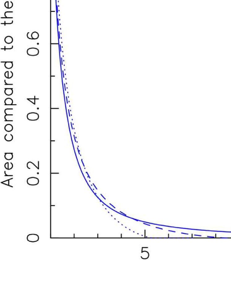
Figure 13: Fractional cross-section as a function of total magnification produced for our model disk-plus-bulge galaxy, with relative orientation $\phi=1.55$.

We then compute the fractional cross-section of the lens having a magnification higher or equal than a given threshold, Fig. 14, as explained in Section 3. With a source size of $r_{\rm e}=0.5$ kpc, we see that for a low magnification threshold ($\mu>8$), the maximum is at $\phi=1.25$ and not at $\phi=1.57$ as we expected. Increasing the threshold magnification, the maximum does shift to $\phi=1.57$. Increasing the misalignment $\phi$, regions of higher magnification but smaller fractional area appear, while at the same time the astroid caustic cross-section decreases. By considering higher magnification thresholds, we focus on more the higher magnification regions. For example, at $\phi=1.25$, the caustic presents two relatively large swallowtails, which are regions of medium-high magnification. For higher magnification thresholds (e.g. $\mu>15$), the swallowtail regions (and indeed the four cusp regions) no longer provide significant cross-section, and the maximum shifts to the butterfly regions (and the region where they overlap). However, this region is correspondingly smaller, and the cross-section decreases to just $\sim 5\times 10^{-3}$ of the multiple imaging area.

These considerations can be used to try and estimate the fraction of butterfly configurations we can observe. The problem for the swallowtails is to find a magnification threshold which isolates these regions (and separates them from the effects of the 4 cusps). The butterfly regions are more cleanly identified in this way: only the place where the two butterflies overlap can give rise to such a small fractional area yet high magnification. When estimating butterfly abundance in Section 7, we will make use of the approximate fractional cross-sectional area of $\sim 5\times 10^{-3}$. For the swallowtails, we note that these form over a wider range of misalignment angles, perhaps $\pm 0.5$ rad from anti-alignment compared to $\pm 0.05$ rad for butterfly formation: we predict very roughly that we would find ten times more swallowtails than butterflies just from their appearing for a ten times wider range of disk/bulge misalignments.

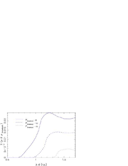
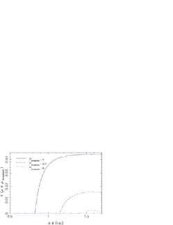
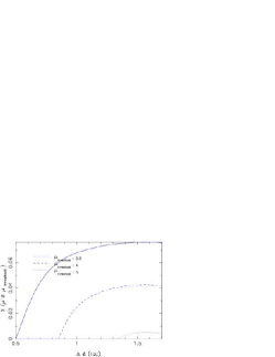
Figure 14: Fractional cross-section area giving total magnification greater than a given threshold, as a function of disk/bulge misalignment angle. We consider our 3 fiducial sources, from left to right: $r_{\rm e}=0.5,1.5,2.5$ kpc

5.2 Galaxies with a satellite

As illustrated in section 4.1 with the system SDSSJ0808$+$4706 and SDSSJ0956$+$5100, main galaxies can have small satellites, relatively close. We expect these satellite to perturb the caustic structures, and perhaps give rise to higher order catastrophes (e.g. C+K04).

5.2.1 Model

We model a system comparable to SDSSJ0808$+$4706, i.e. a main galaxy with a small satellite, by two NIE profiles (with very small cores). The model parameters were set as follows:

Type	$\sigma$	$\epsilon_{\rm p}^{\prime}$	$r_{\rm c}$	$\theta_{1}$	$\theta_{2}$	$\phi$
NIE	236.	0.05	0.05	0	0	1.3
NIE	80.	0.15	0.01	-0.735	1.81	-0.3

where $\sigma$ is in km s^-1, $r_{\rm c}$ in kpc, $\theta$ in arcseconds and $\phi$ in radians.

The redshifts of the lens and source planes were set at $z_{\rm d}=0.2195$ and $z_{\rm s}=1.0215$ (to match those of SDSSJ0808$+$4706). We arbitrarily chose the velocity dispersion of the satellite to be one third that of the main galaxy, and used a double-peaked source to better reproduce the arcs seen in SDSSJ0808$+$4706.

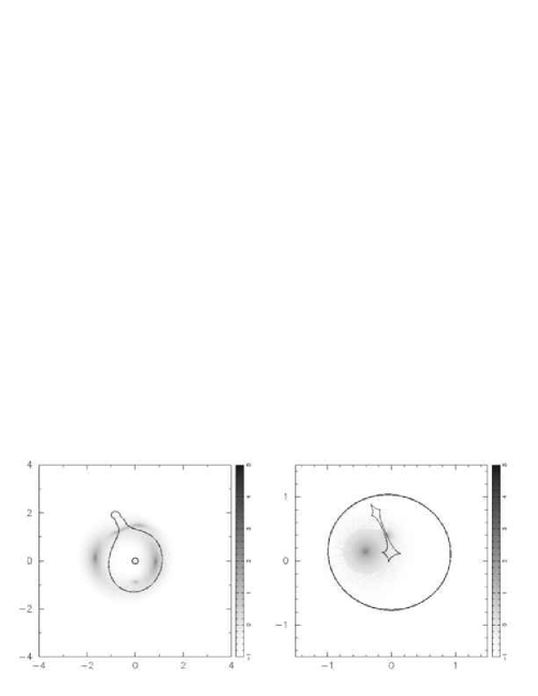
Figure 15: Critical curves and caustics for our model of SDSSJ0808$+$4706, with predicted images overlaid.

5.2.2 Critical curves, caustics and image configurations

The critical curves and caustics for this model system are shown in Fig. 15. The two astroid caustics merge to give an astroid caustic with six cusps instead of four, a beak-to-beak metamorphosis (see section 2.2).

In Fig. 16, we present the beak-to-beak calamity image configuration by slightly adjusting the velocity dispersion parameter of the satellite from $\sigma=80$ km s^-1 to $\sigma=67.7$ km s^-1. The image configuration of the beak-to-beak configuration is the merging of three images in a straight arc (we refer also to Kassiola et al. 1992, who discuss the beak-to-beak in order to explain the straight arc in Abell 2390). The beak-to-beak calamity does not lead to higher magnification (compared to the cusp catastrophes), as it is still the merging of just three images.

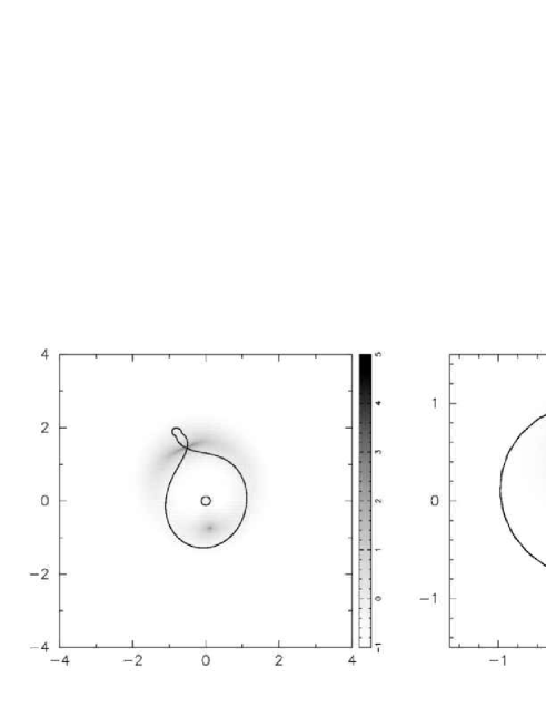
Figure 16: Critical curves and caustics for a model main galaxy plus satellite lens, presenting a beak-to-beak calamity, and a resulting image configuration.

As the lens potential of the satellite increases, the caustics become more complex; such lenses are better classified as “binary” and are studied below in Section 6. On the other hand, small (and perhaps dark) satellite galaxies are expected to modify the lensing flux ratio (e.g. Shin & Evans, 2008b): such substructure can easily create very local catastrophes such as swallowtails (Bradač et al., 2004a), which may be observable in high resolution ring images, as discussed in the previous section (Koopmans, 2005; Vegetti & Koopmans, 2009).

6 Complex lenses

We expect group and cluster-scale lenses to produce higher multiplicities, higher magnifications, and different catastrophes. Motivated by two SL2S targets, SL2SJ1405$+$5502 and SL2SJ0859$-$0345, and the cluster Abell 1703, we first study a binary system, and the evolution of its caustics with lens component separation and redshift, and the apparition of elliptic umbilic catastrophes. Then we illustrated a four-lens component system based on the exotic SL2SJ0859$-$0345 lens. Finally, we study the cluster Abell 1703, which presents an image system characteristic of a hyperbolic umbilic catastrophe.

6.1 Binary lenses

6.1.1 Model

Given the asymmetry of the pair of lens galaxies visible in SL2SJ1405$+$5502 (Section 4.2), we expect the critical curves and caustics to be quite complex. We first make a qualitative model of the lens, using the following mass components:

type	$\sigma$	$\epsilon_{\rm p}^{\prime}$	$r_{\rm c}$	$\theta_{1}$	$\theta_{2}$	$\phi$
NIE	250	0.06	0.1	0.0774	-0.55	1.5
NIE	260	0.04	0.1	-0.0774	0.55	-0.6

where $\sigma$ is in km s^-1, $r_{\rm c}$ in kpc, $\theta$ in arcseconds and $\phi$ in radians. The redshifts chosen are $z_{\rm d}=0.6$ and $z_{\rm s}=1.2$, reasonable estimates for the SL2S objects. As Fig. 17 shows, the model-predicted image configuration matches the observed images fairly well. We note the presence of a predicted faint central image, which may be responsible for some of the brightness in between the lens galaxies in Fig. 8.

We now explore more extensively this type of binary system. We note that the galaxies don’t need to have any ellipticity or relative mis-alignment in order to have an asymmetric potential. We define a simple binary lens model consisting of two identical non-singular isothermal spheres of $\sigma=250$ km s^-1 and core radii of 100 pc, $z_{\rm d}=0.6$ and $z_{\rm s}=1.2$.

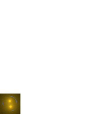
Figure 17: Top: mass distribution of our model of SL2SJ1405$+$5502, and surface brightness of the predicted images. Bottom: critical curves and caustics

6.1.2 Critical curves, caustics and image configurations

In a recent paper, Shin & Evans (2008a) studied strong lensing by binary galaxies, noting the appearance of several catastrophes. Even with isothermal spheres instead of the ellipsoids used in modelling SL2SJ1405$+$5502 above, the binary system can produce an inner astroid caustic with two “deltoid” (three-cusped) caustics (Suyu & Blandford, 2006). The latter characterize an elliptic umbilic metamorphosis, and can be seen in Fig. 19 as the small source-plane features in the right-hand panel, lying approximately along the $\theta_{1}$-axis. The general caustic structure is the result of the merging of the two astroid caustics belonging to the two galaxies.

Shin & Evans (2008a) studied the different metamorphoses undergone as the two mass components are brought closer together. In order to give a further illustration of the caustic structure, we show in Fig. 18 the evolution with source redshift of the caustics behind our binary model system for a given separation $\Delta\theta=1.5^{\prime\prime}$. Plots like this emphasise the three-dimensional nature of the caustic structure, slices of which are referred to as “caustics” in the gravitational lensing literature. This is equivalent to the evolution with separation, since the important parameters are the ratio of the Einstein radii to the separation $\frac{\theta_{E;1,2}}{\Delta\theta}$ and the Einstein radius increases with the redshift. The condition to obtain an elliptic umbilic catastrophe with two isothermal spheres is given by Shin & Evans (2008a),

$$\Delta\theta=\sqrt{\theta_{E,1}^{2}+\theta_{E,2}^{2}}.$$ (10)

At low source redshift, we observe a six-cusp astroid caustic (the aftermath of a beak-to-beak calamity at the merging of the two four-cusp caustics). As the source redshift increases, we observe another two beak-to-beak calamity (the system is symmetric) leading to two deltoid caustics, with the beak-to-beak calamity again marking a transition involving the gain of two cusps. These deltoid caustics then shrink two points, the two elliptic umbilic catastrophes visible at around $z_{s}=1.6$. Beyond this source redshift we then observe two different deltoid caustics (with the elliptic umbilic catastrophe marking the transition between one deltoid and the next). For clarity, we have not represented the outer caustics until the deltoid caustics meet these curves to form a single outer caustic and a lips with two butterflies. In Fig. 19 we present an “elliptic umbilic image configuration,” where four images merge in a Y-shaped feature – yet to be observed in a lens system.

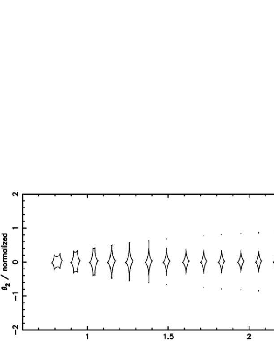
Figure 18: Evolution of the caustics with source redshift behind a fixed-separation binary lens system.

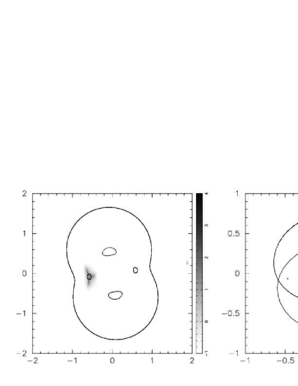
Figure 19: An “elliptic umbilic image configuration.”

The abundance of such image configurations can be estimated very roughly from their fractional cross-section. We estimate geometrically the fractional cross-section of the deltoid caustics in our model system, compared to the multiple imaging area, as being around $10^{-3}$.

6.1.3 Magnification

In order to study the magnification provided by such binary lenses, we again plot the fractional cross-section area with magnification above some threshold, against source redshift. The reference cross-section was taken to be that where the magnification is $\geq$ 3, which corresponds roughly to the multiple imaging area. We make this plot for our three fiducial sources. We first note that the cross-section for a magnification of 10 is quite big ($\sim$0.2): here is a high probability of attaining a high total magnification with such lenses. This probability persists even with large source sizes, although the cross-section for even higher magnification does decrease quite quickly.

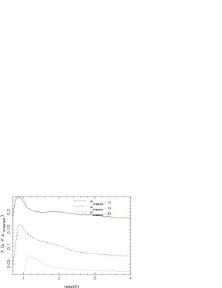
(a) $r_{\rm e}$ = 0.5kpc

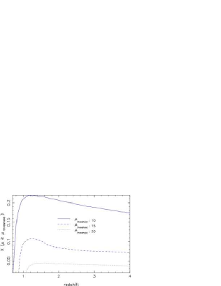
(b) $r_{\rm e}$ = 1.5kpc

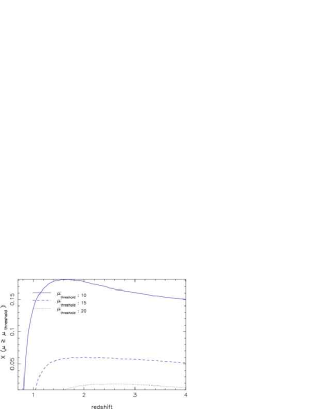
(c) $r_{\rm e}$ = 2.5kpc

Figure 20: Fractional cross-section for magnification higher than a given threshold (compared to area with $\mu\geq 3$) for the binary lens model. We consider 3 fiducial source sizes, from left to right: $r_{\rm e}=0.5,1.5,2.5$ kpc.

For small sources, $r_{\rm e}=0.5$ kpc, the pair of two cusps meeting in a beak-to-beak metamorphosis dominates the magnification $\simeq 10$ cross-section, with the maximum cross-sectional area occurring when the two cups are close but before the beak-to-beak calamity itself. Re-plotting the same small source cross-section with higher magnification thresholds (25, 30, 34, 40, Figs. 20 and 21), we see that the magnification $\simeq 30-40$ cross-section is dominated by the deltoids and their neighbouring cusps. To reach even higher magnifications requires a very high redshift (and hence small in solid angle) source placed at the center of the main astroid.

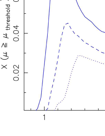
Figure 21: As Fig. 20, but showing higher magnification thresholds.

6.1.4 Two merging galaxies

As an extreme case of the binary system illustrated above, we briefly consider two merging galaxies. The model used is similar except that we use elliptical profiles with $\epsilon_{\rm p}^{\prime}=0.2$ instead of spheres.

In Fig. 22, we plot the convergence and an enlarged view of the caustics for a mass component separation of $\Delta\theta=0.4$ arcseconds and a relative orientation $\phi=1.55$. When we vary the orientation, the fold breaks leading to a swallowtail, then a butterfly and then a region of nine-images multiplicity (as presented in the Fig. 22), similar to that seen in the disk and bulge model Section 5.1. In Fig. 23, we then plot the convergence, the critical curves and the caustics for zero separation and a relative orientation of $\phi=1.2$, as might be seen in a line-of-sight merger or projection. This model has boxy isodensity contours (as also seen in the critical curves), while the caustics include two small butterflies. This model is therefore a a physical way to obtain the boxiness needed to generate such catastrophes (e.g. Evans & Witt, 2001; Shin & Evans, 2008a).

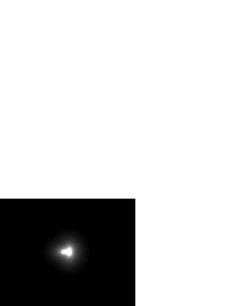
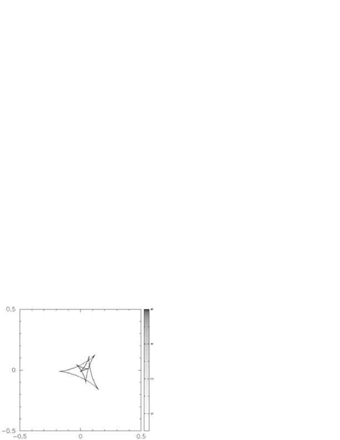
Figure 22: Two elliptical galaxies with a fixed separation $\Delta\theta=0.4$ arcseconds and $\phi=1.55$ radians. Lens convergence map left, and a zoomed-in view of the astroid caustic in the source plane right.

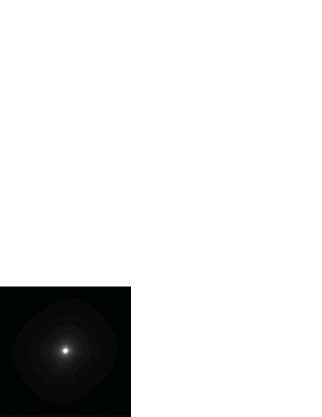
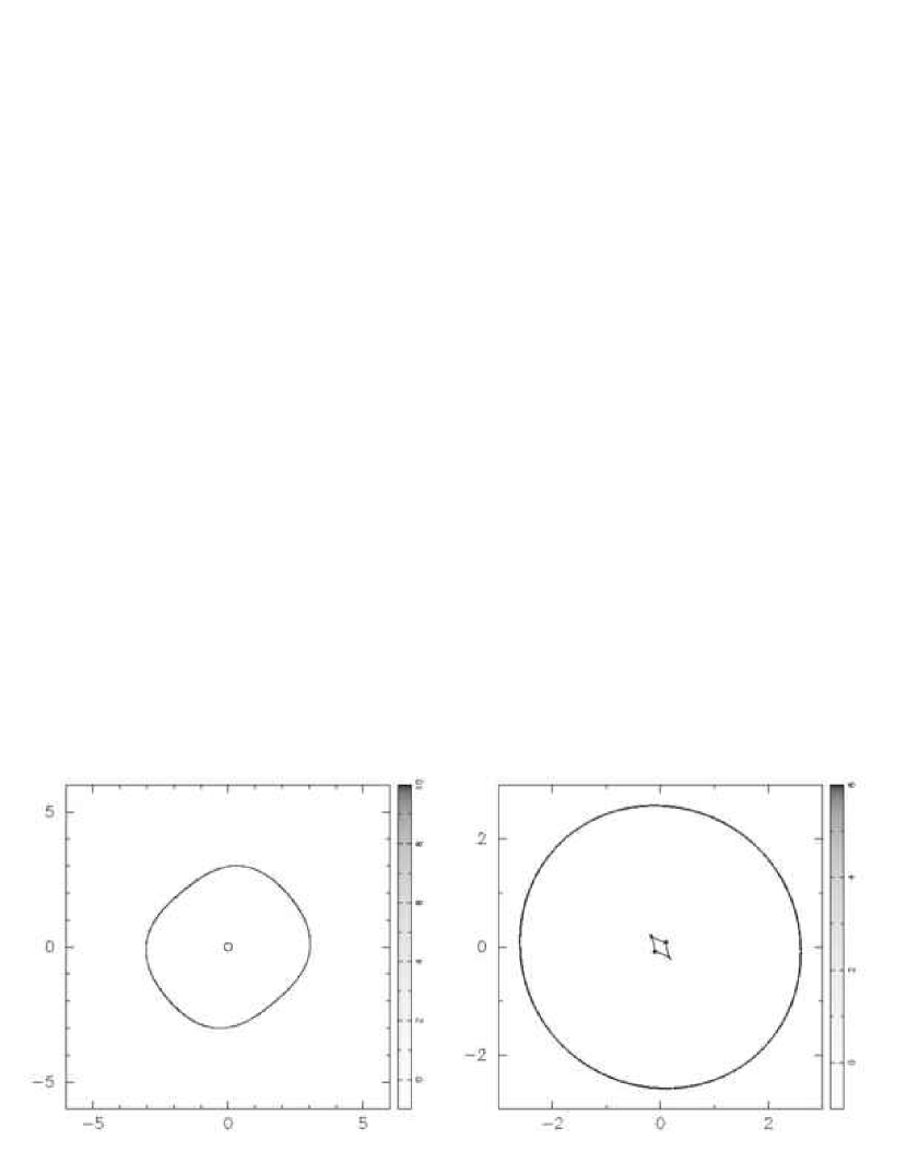
Figure 23: Two elliptical galaxies with a relative orientation of 1.2 radians, separation $\Delta\theta=0$ arcsec.

6.2 A four-component lens system: SL2SJ0859$-$0345

6.2.1 Model

SL2SJ0859$-$0345 is an example of a lens with still more complex critical curves and caustics; we represent it qualitatively with the following four-component model:

type	$\sigma$	$\epsilon_{\rm p}^{\prime}$	$r_{\rm c}$	$\theta_{1}$	$\theta_{2}$	$\phi$
NIS	250	0.0	0.1	-1.3172	0.87	0
NIE	330	0.1	0.1	1.9458	0.12	1.2
NIE	200	0.1	0.1	-1.2872	-2.17	-0.3
NIS	120	0.0	0.1	0.6885	1.17	0

where once again $\sigma$ is in km s^-1, $r_{\rm c}$ in kpc, $\theta$ in arcseconds and $\phi$ in radians. The redshifts chosen were $z_{\rm d}=0.6$ and $z_{\rm s}=2$. The velocity dispersions and the ellipticities were chosen to reflect the observed surface brightness. In Fig. 24 we show our best predicted images, for comparison with the real system in Fig. 9.

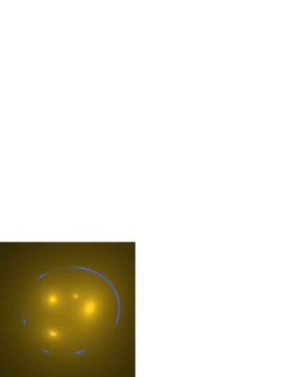
Figure 24: Convergence and predicted images for a qualitative model of SL2SJ0859$-$0345, showing the 4 lens components and complex oval system of arcs.

6.2.2 Critical curves, caustics and image configurations

In Fig. 25, we present an array of different image configurations produced by varying the source position, illustrating what might have been. Several different multiplicities are possible, including an elliptic umbilic image configuration. The caustic structure is composed of two outer ovoids, a folded astroid caustic, a lips, and a deltoid caustic. The highest image multiplicity obtained is nine (in practice eight images, and referred to as an octuplet). We also plot the evolution of these caustics with source redshift in Fig. 26: several beak-to-beak calamities result in the extended and folded-over central astroid caustic, while the elliptic umbilic catastrophe occurs at around $z_{\rm s}\simeq 2.3$. As a caveat, this four-lens model is in one sense maximally complex: any smooth group-scale halo of matter would act to smooth the potential and lead to somewhat simpler critical curves and caustics. However, it serves to illustrate the possibilities, and may not be far from a realistic representation of such compact, forming groups.

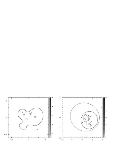
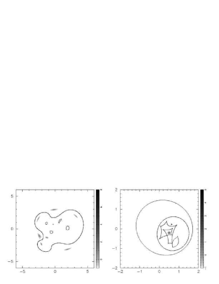
Figure 25: Alternative histories for the SL2SJ0859$-$0345 system: the image configurations (left) and multiplicities resulting from various source positions (right). Left column, from top to bottom: 1. Double image, of a source in the first outer caustic. 2. Quad: second outer caustic. 3. Sextuplet: outer astroid caustic. 4. Quad: lips caustic. 5. Octuplet: inner-astroid caustic. Right column, from top to bottom: 1. Sextuplet, including 4 merging images of an elliptic umbilic configuration: source in a deltoid caustic. 2. Octuplet: source at the astroid fold crossing point. 3, 4, 5. Octuplets: sources on each of the three inner-astroid cusps.

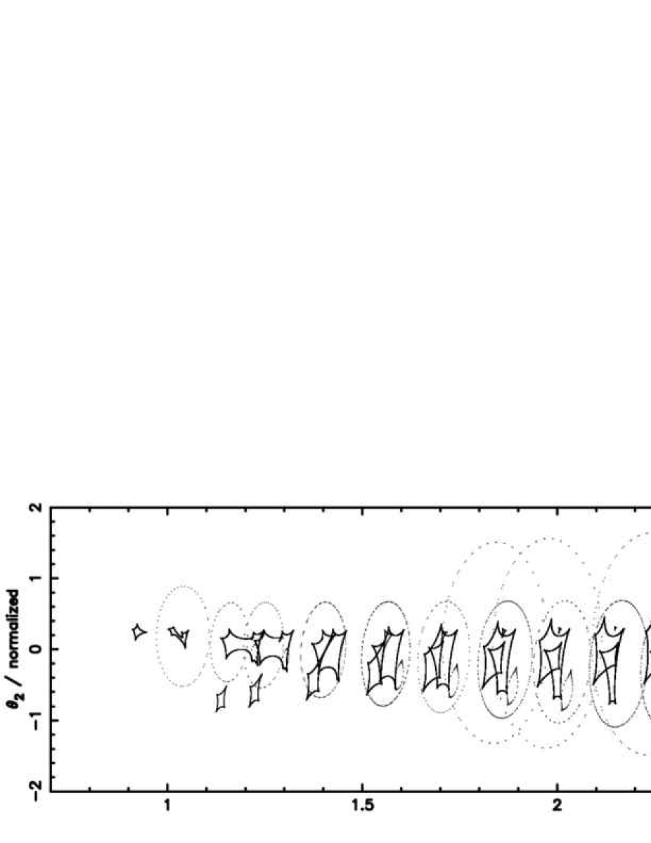
Figure 26: Evolution of the caustics with source redshift for our qualitative model of SL2SJ0859$-$0345. The ovoid outer curves are sometimes only sparsely sampled by the adaptive mesh code used to compute the magnification maps (see appendix).

6.2.3 Magnification

We choose to not discuss extensively the magnification of this system, having already examined the available magnifications in the simpler instances of the various caustic structures in previous sections. Nevertheless, we would still like to know if the deltoid caustic (when we are close to an elliptic umbilic catastrophe) can lead to a higher magnification than other regions of the source plane. In order to do that, we compute the total magnification for two particular positions of the source: in the central astroid caustic (leading to eight observable images in a broken Einstein ring, bottom left panel of Fig. 25), and in the deltoid caustic (top right panel of Fig. 25).

We again consider our three fiducial exponential sources ($r_{\rm e}=\{0.5,1.5,2.5\}$ kpc. The central position leads to magnifications of $\mu\simeq\{55,39,27\}$ respectively, and for the deltoid position we obtain a total magnification of $\mu\simeq\{49,33,24\}$. The deltoid caustic again does not give the maximum total magnification – it is a region of image multiplicity seven, while the central astroid caustic of multiplicity nine. However, the deltoid does concentrate, as a cusp does, the magnification into a single merging image object. In the next section we will see an example of how such focusing by a higher order catastrophe leads to a highly locally-informative image configuration.

6.3 Abell 1703

Fig. 27 shows the central part of the cluster Abell 1703, and its critical curves and caustics as modeled by Limousin et al. (2008b). This elliptical cluster, modelled most recently by Oguri et al. (2009) and Ric++09, contains an interesting wide-separation ($\simeq 8$ arcsec) 4-image system (labelled 1.1–1.4 in the left-hand panel of Fig. 27). This “central ring” quad has a counter-image on the opposite side of the cluster (labelled 1.5). Two red galaxies lie inside the ring; they are marked as two red dots in the central panel of Fig. 27.

Explaining the central ring as one image of a double system being split by the two red galaxies is difficult; in the Limousin et al. (2008b) mass model they are represented as isothermal spheres with velocity dispersion $\simeq 100$ km s^-1 each. The wide separation of the ring is a feature of the cluster-scale mass distribution, as we now show. We made a rough modeling of the cluster using a NIE profile with velocity dispersion of $\sim$ 1200 km s^-1, a core radius of $\sim$ 30 kpc, and an ellipticity of the potential of $\epsilon_{\rm p}^{\prime}=0.2$. This single halo model reproduces the central ring image configuration very well. We show the predicted images, critical curves and caustics in the upper panels of Fig. 28. This image configuration is associated with a hyperbolic umbilic catastrophe; one can see in the right-most panel of Fig. 27 and more clearly in he corresponding panel of Fig. 28 that the source lies very close to the point where the ovoid and astroid caustics almost touch. Were the source actually at the catastrophe point, the four images of the central ring would be merging; as it is, we see the characteristic pattern of a hyperbolic umbilic image configuration. As far as we know this is the first to have ever been observed.

When we add the two $\sigma=100$km s^-1 SIE galaxies inside the central ring (lower panels of Fig. 28), the central ring system is perturbed a little. This perturbation allowed Limousin et al. (2008b) to measure them despite their small mass, illustrating the notion that sources near higher order catastrophes provide opportunities to map the local lens mass distribution in some detail. Indeed, this image system provides quite a strong constraint on the mass profile of the cluster (Limousin et al., 2008b).

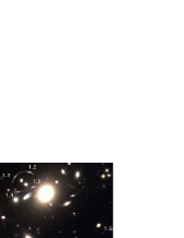
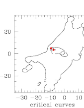
Figure 27: Abell 1703 and the lens model modeled of Limousin et al. (2008b) Left: the core of the cluster observed with HST/ACS (Stott, 2007). The image is approximately 40 arcsec wide. Critical curves (centre) and caustics (right) in the lens model of Limousin et al. (2008b). The two galaxies inside the central ring are represented by two filled red circles.

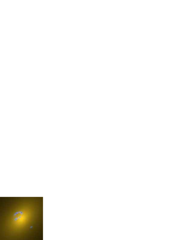
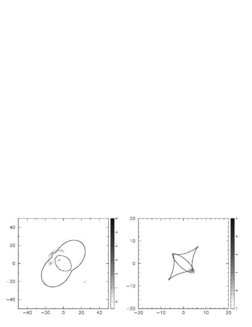
Figure 28: Simple models for understanding Abell 1703, with predicted images (left), critical curves (centre) and caustics (right). The effect of the two galaxies inside the central ring is shown in the lower panels; they are absent from the model in the upper panels.

6.3.1 An even simpler model

To try and estimate the abundances of such hyperbolic umbilic image configurations, we consider a slightly more representative (but still very simple) model of a cluster: cluster and its brightest cluster galaxy (BCG), both modelled by a NIE profile. The parameters used are taken after considering the sample of Smith et al. (2005) who modelled a sample of clusters using NIE profiles. The model is as follows:

type	$\sigma$	$\epsilon_{\rm p}^{\prime}$	$r_{\rm c}$
NIE - Cluster	900	0.2	80
NIE - BCG	300	0.2	1

where $\sigma$ is in km s^-1 and $r_{\rm c}$ is in kpc.

6.3.2 Critical curves, caustics and image configurations

Using a simple NIE profile, we can obtain an hyperbolic umbilic catastrophe, provided that the central convergence is sufficiently shallow (i.e. a significant core radius is required), and sufficiently elliptical. Kormann et al. (1994) give a criterion for a NIE lens to be capable of generating a hyperbolic umbilic catastrophe:

$$b_{\rm c}=\dfrac{q^{2/3}}{2},$$ (11)

where $b_{\rm c}$ is the core radius in units of the Einstein radius. and the axis ratio $q$ refers to the mass distribution and not the lens potential. Kassiola & Kovner (1993) also discuss elliptical mass distributions and elliptical potentials, and describe the different metamorphoses when varying the core radius.

We show the evolution of this model’s caustics with source redshift in Fig. 29. At low redshift, the caustic structure consists of two lips (with relative orientation of 90 degrees); as $z_{\rm s}$ increases, the inner lips becomes bigger and meets the outer lips in a hyperbolic umbilic catastrophe. The hyperbolic umbilic metamorphosis conserves the number of cusps: at higher source redshift, we see the familiar (from elliptical galaxies) outer ovoid caustic with an inner astroid caustic.

In the light of these considerations, we don’t expect hyperbolic umbilic catastrophes to be generic in elliptical galaxy lenses, as the central convergence is not sufficiently shallow. However, this catastrophe point should be present behind many clusters, as the combination of a BCG and a cluster with appropriate core radii and ellipticities can lead to the central convergence and ellipticity required. Of course the hyperbolic umbilic image configuration is more likely to happen than the catastrophe itself. Indeed, as Fig. 29 shows, the hyperbolic umbilic image configuration can occur over a wide range of source redshift.

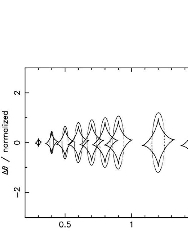
Figure 29: Evolution of a simple elliptical cluster lens caustics with source redshift. The closeness of the cusps to the outer ovoid caustic persists over a wide range of redshifts.

6.3.3 Magnification

Fig. 30 shows the fractional cross-section area of our NIE cluster model (at $z_{\rm d}=0.28$) as a function of magnification threshold. Here, the area of the source plane providing total magnification greater than $\mu$ is compared to the area providing total magnification greater than $\mu\geq 15$, which is approximately the area of the astroid caustic. We consider again our fiducial exponential sources, and observe that the system produces some very high magnifications. Analyzing the different convolved maps of source plane magnification, we find that it is indeed the regions close to the hyperbolic umbilic catastrophes that provide the highest magnifications. For $r_{\rm e}=0.5$ kpc, the cross-section for $\mu\geq 100$ is entirely due to the two regions close to the catastrophe. We obtain the same result for the two other sources (respectively $\mu\simeq 75$ and $\mu\simeq 25$ for $r_{\rm e}=1.5$ and $2.5$ kpc): it is likely that A1703 is magnifying its source by something like these factors. Fig. 30 shows that the region with a characteristic magnification of a hyperbolic umbilic catastrophe is around 1–2% of the multiple-imaging area.

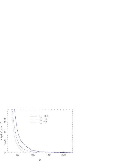
Figure 30: Fractional cross-section (relative to the area with magnification $\mu\geq 15$) as a function of the threshold magnification for our simple NIE cluster model.

7 The abundance of higher-order catastrophes

In the previous sections, we have illustrated a range of “exotic” lenses, systems presenting higher-order catastrophes such as swallowtails, butterflies, elliptic umbilics and hyperbolic umbilics, and their related metamorphoses. In this section we make the first very rough approximations of the abundances of lenses showing such exotic image configurations.

Procedure. For each given type of lens, we first estimate the basic abundances of the more common, lower magnification configurations, based on the number densities observed so far in SLACS and SL2S. We then estimate, for a given source redshift, the fractional cross-section area for production of the desired image configuration. To do this we consider both a) the information provided by the magnification maps and their associated fractional cross-sectional areas, and b) our rough estimates of the “area of influence” of the relevant caustic feature. Finally, we estimate the typical window in source redshift for which the image configuration is obtainable, and hence the fraction of sources lying at a suitable position along the line of sight. The product of these two fractions with the basic abundance gives us an order-of-magnitude estimate of the number density of exotic lenses detectable in a future imaging survey (which we take to cover $\sim 10^{4}$ square degrees).

Galaxy scales. On galaxy scales, we expect some 10 strong gravitational lenses observable per square degree, provided the image resolution is high enough: this is approximately what is found in the COSMOS (Faure et al., 2008) and EGS (Moustakas et al., 2007) surveys. The majority of these lens galaxies are massive ellipticals, as expected (Turner et al., 1984). In the larger SLACS sample of similar galaxy-galaxy lenses, the fraction of systems showing strong evidence of a disk component is approximately 10%, while only one or two (a few percent) have massive satellites within the Einstein radius (Bolton et al., 2008). Making the link between galaxy-scale lenses expected in imaging surveys and the lenses found by the SLACS survey should be done with care, but it is not unreasonable to start from this extrapolation – especially in the light of the SLACS studies demonstrating the normality of the lens galaxies relative to the parent massive galaxy population (Treu et al., 2006; Tre++09). This gives us basic abundances of disky lenses and binary/merging lenses of $\sim 1$ and $\sim 0.1$ per square degree respectively. This is what we might expect a space-based survey to recover; the number visible from the ground will be much reduced by the image resolution.

Therefore, our estimate of the abundance of butterflies is $1\times(10/180)\times 0.001\sim 5\times 10^{-5}$ per square degree, where $10/180$ is the angular range where we can expect butterflies, 0.001 is our estimation of the cross-section of the butterflies and nine-image multiplicity regions from Section 5.1. Note that we have optimistically considered a uniform distribution of disk-bulge misalignments: this abundance might be taken as an upper limit for these types of lens mass distributions. We expect to have roughly 10 times more swallowtails, since the range of misalignment angles leading to swallowtails is $\sim 10$ times greater than that for butterflies. We therefore obtain an upper limit of $\sim 1$ observable disk/bulge butterfly on the sky, and $\sim$10 disk/bulge swallowtails.

Group scales. On group scales, we might expect the ground-based surveys to be as complete as those from space. Moreover, the depth of the CFHT Legacy Survey images is comparable to that expected from future surveys such as that planned with LSST (which will cover 2 orders of magnitude more sky area). Extrapolating the number of group-scale gravitational lenses from the SL2S survey (Cabanac et al., 2007) is therefore a reasonable starting point. The observed abundance of group-scale lenses is $\sim 0.1$ per square degree, and perhaps a third show multiple mass components within the Einstein radius. To order of magnitude we therefore estimate the basic abundances of compact group lenses as $\sim 0.01$ per square degree.

The two systems studied here show a variety of complex caustic structure. In the case of the binary systems in Section 6.1, we estimated geometrically the fractional cross-section of a deltoid caustic to be $\sim$ 10^-3 over a wide redshift range. We therefore obtain an order of magnitude estimate of $0.01\times 10^{-3}\sim$10^-5 per square degree for the abundance of elliptic umbilic image configurations, or approximately one observable Y-shaped image feature in our future survey. This cross-section area is unlikely to be very different (depending on the lens) to that for the production of swallowtails and butterflies by group lenses. A Monte Carlo simulation would perhaps be the best way to estimate these abundances more accurately.

Clusters. For clusters, as shown in section 6.3.2, the properties needed to obtain an hyperbolic umbilic catastrophe are well understood: the problem lies in estimating the ranges of ellipticities, convergences and core radii of the cluster and BCG mass distributions that combine to provide a sufficiently shallow inner density slope for the system to generate a hyperbolic umbilic. As a first attempt, we consider the distribution of cluster lens potential ellipticities estimated from numerical simulations: this is approximately a Gaussian with mean 0.125 and width 0.05 (Marshall 2006, following Jing & Suto 2002). In general the BCG increases the central mass slope (decreasing the core radius of an effective NIE profiles), such that we need high ellipticity in order to be close to an hyperbolic umbilic catastrophe. We estimate that only the 1–10% highest ellipticity clusters will meet this criterion. Our qualitative analysis in Section 6.3 suggests that once the ellipticity and density profile condition is met then the hyperbolic umbilic metamorphosis is slow with source redshift. The fractional cross-section area of this “hyperbolic umbilic region” is approximately 2%. As the number of cluster lenses is expected to be $\sim 0.1$ per square degree, we estimate the abundance to be $\sim 10^{-4}$ per square degree, again predicting $\sim 1$ hyperbolic umbilic catastrophe image configuration per sky survey. A question comes to mind: is Abell 1703 the only hyperbolic umbilic gravitational lens we will ever see?

Discussion. Throughout this work we have focused on the most abundant sources, the faint blue galaxies, and tried to account for their finite size when estimating magnifications and now abundances. To first order this should take care of any magnification bias. However, for the less common point-like sources (such as quasars and AGN) it is possible that magnification bias may play a much more important role. Investigation of this effect would be a good topic for further work. The sensitivity of galaxy-scale gravitational lensing of point sources to small-scale CDM substructure (e.g. Mao & Schneider, 1998; Dalal & Kochanek, 2002; Bradač et al., 2004a) is such that more investigation of the exotically-lensed quasar abundance is certainly warranted. There are similar, but perhaps more constraining, relations between the signed fluxes of images of sources lying close to higher order catastrophes (Aazami & Petters, 2009) as there are for folds and cusps (Keeton et al., 2003, 2005).

Another possibility that might be included in a more complete analysis of exotic lens abundance is that of generating higher order catastrophes with multiple lens planes, a topic studied by (Kochanek & Apostolakis, 1988). If a substantial fraction of the observed group-scale lenses are in fact due to superpositions of massive galaxies rather than compact groups this could prove a more efficient mechanism for the production of higher order catastrophes.

8 Conclusions

Inspired by various samples of complex lenses observed, and with future all-sky imaging surveys in mind, we have compiled an atlas of realistic physical gravitational lens models capable of producing exotic image configurations associated with higher-order catastrophes in the lens map. For each type of lens considered, we have investigated the caustic structure, magnification map, and example image configurations, and estimated approximate relative cross-sections and abundances. We draw the following conclusions:

• Misalignment of the disk and bulge components of elliptical galaxies gives rise to swallowtail (for a wide range of misalignment angles) and butterfly catastrophes (if the misalignment is close to 90 degrees). The image configuration produced by the butterfly caustic would be observed as a broken (8-image) Einstein ring.

• The central nine-imaging region has cross-section $\sim 10^{-3}$ relative to the total cross-section for multiple imaging; combining this with rough estimates of the abundance of such disky lens galaxies in the SLACS survey, we estimate an approximate abundance of $\lesssim 1$ such butterfly lens per all-sky survey. We estimate that the swallowtail lenses could be $\sim 10$ times more numerous.

• Binary and merging galaxies produce elliptic umbilic catastrophes when the separations of the mass components are comparable to their Einstein radii. The configuration formed when the source lies within the deltoid caustic is a Y-shaped pattern of 4 merging images between, but offset from, the two lenses.

• In this case the deltoid caustic does not provide the maximum total magnification available to the lens; the relevant cross-section must be estimated from the area within the deltoid. We find the relative cross-section to also be $\sim 10^{-3}$, leading to an approximate abundance of $\sim 1$ binary galaxy elliptic umbilic lens per all-sky survey.

• More complex group-scale lenses, of the kind being discovered by the SL2S survey, offer a wide range of critical points in their caustics, and so are a promising source of exotic lenses. For example, our model of SL2SJ0859$-$0345 shows an elliptic umbilic catastrophe at around $z=2.4$. At present, our understanding of the distribution of group-scale lens parameters, and the extreme variety of caustic structure prevents us making accurate estimates of the exotic lens abundance for these systems.

• As noted by previous authors, elliptical clusters with appropriate inner density profile slopes produce hyperbolic umbilic catastrophes. We find that just such a simple model is capable of reproducing the central ring image configuration of Abell 1703, demonstrating the source to lie close to a hyperbolic umbilic point. The total magnification of this source could be $\sim 100$, depending on the source size.

• Despite the rather general properties of clusters needed to produce such image configurations, we estimate that the all-sky abundance of such hyperbolic umbilic cluster lenses may still only be $\sim 1$.

In some cases, proximity to a catastrophe point does not guarantee maximal magnification. Further studies of the abundances of exotic lenses should explore more advanced diagnostics of catastrophic behavior. While high magnification is certainly a desirable feature of gravitational lenses for some applications (e.g. cosmic telescope astronomy), high local image multiplicity is perhaps the more relevant property for studies of small scale structure in the lens potential, using the information on the gradient and curvature of the mass distribution that is present. The constraining power of the hyperbolic umbilic image configuration in Abell 1703 is a good example of this on cluster scales. The exploitation of the plausible lenses we have predicted here in this way would be an interesting topic for further research.

Appendix A Lens and source models

In this appendix, we describe in a little more detail the different models used throughout the paper: the isothermal profiles to model the lens potentials and the Sersic profiles for the background source galaxies’ light distributions (or for the stellar mass component of a lens galaxy).

For all image simulations in this paper we uses the publically-available glamroc code (Gravitational Lens Adaptive Mesh Ray-tracing of Catastrophes) written by E. A. Baltz. Here we give a very brief introduction to this code and its capabilities.

Each glamroc lens model is made of an arbitrary number of lensing objects on an arbitrary number of lens planes. The individual lensing object all have analytic lens potentials, such that all their derivatives are also analytic. In this way the deflection angles, magnification matrices, and combinations of higher derivatives can be calculated as sums of terms coming from each lens in turn. Higher derivatives are required to identify catastrophes of the lens map, which include all the catastrophes define above. An adaptive mesh is used to improve the resolution either near the critical curves of the lens system or in regions of high surface brightness. Lens types currently implemented include point masses, isothermal spheres with and without core and truncation radii, NFW profiles with and without truncation, and Sersic profiles. For each type, elliptical isopotentials can be used and either boxiness, diskiness and skew added. Sources are modelled with (superpositions of) elliptically-symmetric Sersic profiles.

A.1 Isothermal lenses

Throughout the paper, we used the non-singular isothermal ellipsoid (NIE) model for our lens components. The NIE (three-dimensional) mass density diverges as $\rho\varpropto r^{-2}$; the surface (projected) mass density profile is

$$\Sigma(r)=\dfrac{\sigma}{2G(r^{2}+r_{\rm c}^{2})^{1/2}},$$ (12)

where $r$ is now the projected radius, $r_{\rm c}$ is the core radius, and $\sigma$ is the velocity dispersion of the lens. The core radius is that at which the rising density profile turns over into a uniform distribution in the central region. This type of profile has been shown to be a very good approximation of the lens potential on both galaxy scales (e.g. Koopmans et al., 2006), provided the core radius is very small ($\lesssim 0.1$ kpc), and also on cluster scales, with much larger core radii ($\sim 50.0$ kpc, e.g. Smith et al., 2005). In practice a small core allows more convenient plotting of caustics and critical curves. However, we are careful not to allow cores larger than typically permitted by the data: the non-singular core prevents the infinite de-magnification of the central image, which would be observable.

The NIE model isopotential lines are ellipses with constant

$$r^{2}=(1-\epsilon_{\rm p}^{\prime})x^{2}+(1+\epsilon_{\rm p}^{\prime})y^{2}.$$ (13)

where $x$ and $y$ denote the Cartesian coordinates in the lens plane. The potential is, therefore, a function of $r$ only, and the ellipticity $\epsilon_{\rm p}^{\prime}$ is the ellipticity of this potential. The ellipticity must be carefully chosen in order to keep the potential physically meaningful. Indeed, for $\epsilon_{\rm p}^{\prime}>0.2$ the isodensity contours become dumbbell-shaped (see e.g. Kassiola & Kovner, 1993). BMO09 provide a simple practical solution to this problem: add several (suitably chosen and weighted) elliptical potentials at the same location. Using their algorithm, we are able to model nearly elliptical isodensity contours with ellipticities as large as $\epsilon^{\prime}=0.8$. This allows us to model, for example, the combination of a bulge and a disk in a galaxy. (Note that the NIE model described here is different from that defined by Kormann et al. (1994), where the ellipticity pertains to the mass distribution, not to the lens potential.)

We follow the glamroc notation and use as our main ellipticity definition $\epsilon^{\prime}=\frac{a^{2}-b^{2}}{a^{2}+b^{2}}$, where $a$ and $b$ are the major and minor axis lengths of the ellipse in question. This is different from the definition often used in weak lensing, $\epsilon=\frac{a-b}{a+b}$. The relation between these two definitions of the ellipticity is $\epsilon^{\prime}=\frac{2\epsilon}{1+\epsilon^{2}}$.

A.2 Sersic sources

The Sersic power law profile is one of the most frequently used in the study of galaxy morphology. It has the following functional form (e.g. Peng et al., 2002),

$$I(r)=I_{\rm e}\exp{\left[-\kappa\left(\left(\dfrac{r}{r_{\rm e}}\right)^{1/n}-1\right)\right]},$$ (14)

where $I_{\rm e}$ is the surface brightness at the effective radius $r_{\rm e}$. The parameter $r_{\rm e}$ is known as the effective, or half-light, radius, defined such that half of the total flux lies within $r_{\rm e}$. The parameter $n$ is the Sersic index: with $n=1/2$ the profile is a Gaussian, $n=1$ gives an exponential profile typical of elliptical galaxies, and $n=4$ is the de Vaucouleurs profile found to well-represent galaxy bulges. We compared these three standard profiles when exploring the observability of exotic lenses in the text.

The half-light radius is an important parameter when considering the observable magnification of extended sources. For the sizes of the expected faint blue source galaxies, we adopted the size-redshift relation measured by Ferguson et al. (2004). For reference, this gave effective radii of 4.0 kpc (0.5”) at $z_{\rm s}=1$, decreasing to 2.9 kpc (0.35”) at $z_{\rm s}=2$ and 1.7 kpc (0.21”) at $z_{\rm s}=4$. We used sources having equal half-light radii, instead of the same total flux (the relative intensity is, as we explain in the paper, not important as the magnification calculation based on Equation 9 is independent of the total flux of the source).

References

- Aazami & Petters (2009) Aazami, A. B., & Petters, A. O. 2009, J. Math. Phys., 50, 032501
- Aldering et al. (2004) Aldering, S. C. G., et al. 2004, astro-ph/0405232
- Bagla (2001) Bagla, J. S. 2001, in Astronomical Society of the Pacific Conference Series, Vol. 237, Gravitational Lensing: Recent Progress and Future Go, ed. T. G. Brainerd & C. S. Kochanek, 77–+
- Baltz et al. (2007) Baltz, E. A., Marshall, P., & Oguri, M. 2007, ArXiv e-prints, 705
- Blandford & Narayan (1986) Blandford, R., & Narayan, R. 1986, ApJ, 310, 568
- Bolton et al. (2008) Bolton, A. S., Burles, S., Koopmans, L. V. E., Treu, T., Gavazzi, R., Moustakas, L. A., Wayth, R., & Schlegel, D. J. 2008, ArXiv e-prints, 805
- Bolton et al. (2006) Bolton, A. S., Burles, S., Koopmans, L. V. E., Treu, T., & Moustakas, L. A. 2006, ApJ, 638, 703
- Bradač et al. (2004a) Bradač, M., Schneider, P., Lombardi, M., Steinmetz, M., Koopmans, L. V. E., & Navarro, J. F. 2004a, A&A, 423, 797
- Bradač et al. (2004b) —. 2004b, A&A, 423, 797
- Cabanac et al. (2007) Cabanac, R. A., Alard, C., Dantel-Fort, M., Fort, B., Gavazzi, R., Gomez, P., Kneib, J. P., Le Fèvre, O., Mellier, Y., Pello, R., Soucail, G., Sygnet, J. F., & Valls-Gabaud, D. 2007, A&A, 461, 813
- Dalal & Kochanek (2002) Dalal, N., & Kochanek, C. S. 2002, ApJ, 572, 25
- Ellis (1997) Ellis, R. S. 1997, ARA&A, 35, 389
- Evans & Witt (2001) Evans, N. W., & Witt, H. J. 2001, MNRAS, 327, 1260
- Faure et al. (2008) Faure, C., Kneib, J.-P., Covone, G., Tasca, L., Leauthaud, A., Capak, P., Jahnke, K., Smolcic, V., de la Torre, S., Ellis, R., Finoguenov, A., Koekemoer, A., Le Fevre, O., Massey, R., Mellier, Y., Refregier, A., Rhodes, J., Scoville, N., Schinnerer, E., Taylor, J., Van Waerbeke, L., & Walcher, J. 2008, ApJS, 176, 19
- Ferguson et al. (2004) Ferguson, H. C., Dickinson, M., Giavalisco, M., Kretchmer, C., Ravindranath, S., Idzi, R., Taylor, E., Conselice, C. J., Fall, S. M., Gardner, J. P., Livio, M., Madau, P., Moustakas, L. A., Papovich, C. M., Somerville, R. S., Spinrad, H., & Stern, D. 2004, ApJ, 600, L107
- Hennawi et al. (2008) Hennawi, J. F., Gladders, M. D., Oguri, M., Dalal, N., Koester, B., Natarajan, P., Strauss, M. A., Inada, N., Kayo, I., Lin, H., Lampeitl, H., Annis, J., Bahcall, N. A., & Schneider, D. P. 2008, AJ, 135, 664
- Ivezic et al. (2008) Ivezic, Z., et al. 2008, astro-ph/0805.2366
- Jing & Suto (2002) Jing, Y. P., & Suto, Y. 2002, ApJ, 574, 538
- Kassiola & Kovner (1993) Kassiola, A., & Kovner, I. 1993, ApJ, 417, 450
- Kassiola et al. (1992) Kassiola, A., Kovner, I., & Blandford, R. D. 1992, ApJ, 396, 10
- Keeton et al. (2003) Keeton, C. R., Gaudi, B. S., & Petters, A. O. 2003, ApJ, 598, 138
- Keeton et al. (2005) —. 2005, ApJ, 635, 35
- Keeton et al. (2000) Keeton, C. R., Mao, S., & Witt, H. J. 2000, ApJ, 537, 697
- Kochanek & Apostolakis (1988) Kochanek, C. S., & Apostolakis, J. 1988, MNRAS, 235, 1073
- Koopmans (2005) Koopmans, L. V. E. 2005, MNRAS, 363, 1136
- Koopmans et al. (2006) Koopmans, L. V. E., Treu, T., Bolton, A. S., Burles, S., & Moustakas, L. A. 2006, ApJ, 649, 599
- Kormann et al. (1994) Kormann, R., Schneider, P., & Bartelmann, M. 1994, A&A, 284, 285
- Laureijs et al. (2008) Laureijs, R., et al. 2008
- Limousin et al. (2008a) Limousin, M., Cabanac, R., Gavazzi, R., Kneib, J. P., Motta, V., Richard, J., Thanjavur, K., Foex, G., Crampton, D., Faure, C., Fort, B., Jullo, E., Marshall, P., Mellier, Y., More, A., Pello, R., Soucail, G., Suyu, S., Swinbank, M., Sygnet, J. F., Tu, H., Valls-Gabaud, D., Verdugo, T., & Willis, J. 2008a, ArXiv e-prints
- Limousin et al. (2008b) Limousin, M., Richard, J., Kneib, J.-P., Brink, H., Pelló, R., Jullo, E., Tu, H., Sommer-Larsen, J., Egami, E., Michałowski, M. J., Cabanac, R., & Stark, D. P. 2008b, A&A, 489, 23
- Mao & Schneider (1998) Mao, S., & Schneider, P. 1998, MNRAS, 295, 587
- Marshall (2006) Marshall, P. 2006, MNRAS, 372, 1289
- Marshall et al. (2007) Marshall, P. J., Treu, T., Melbourne, J., Gavazzi, R., Bundy, K., Ammons, S. M., Bolton, A. S., Burles, S., Larkin, J. E., Le Mignant, D., Koo, D. C., Koopmans, L. V. E., Max, C. E., Moustakas, L. A., Steinbring, E., & Wright, S. A. 2007, ApJ, 671, 1196
- Möller et al. (2003) Möller, O., Hewett, P., & Blain, A. W. 2003, MNRAS, 345, 1
- More et al. (2008) More, A., McKean, J. P., More, S., Porcas, R. W., Koopmans, L. V. E., & Garrett, M. A. 2008, ArXiv e-prints
- Moustakas et al. (2007) Moustakas, L. A., Marshall, P., Newman, J. A., Coil, A. L., Cooper, M. C., Davis, M., Fassnacht, C. D., Guhathakurta, P., Hopkins, A., Koekemoer, A., Konidaris, N. P., Lotz, J. M., & Willmer, C. N. A. 2007, ApJ, 660, L31
- Oguri et al. (2009) Oguri, M., Hennawi, J. F., Gladders, M. D., Dahle, H., Natarajan, P., Dalal, N., Koester, B. P., Sharon, K., & Bayliss, M. 2009, ArXiv e-prints
- Peng et al. (2002) Peng, C. Y., Ho, L. C., Impey, C. D., & Rix, H.-W. 2002, AJ, 124, 266
- Petters et al. (2001) Petters, A. O., Levine, H., & Wambsganss, J. 2001, Singularity theory and gravitational lensing (Singularity theory and gravitational lensing / Arlie O. Petters, Harold Levine, Joachim Wambsganss. Boston : Birkhäuser, c2001. (Progress in mathematical physics ; v. 21))
- Rusin et al. (2001) Rusin, D., Kochanek, C. S., Norbury, M., Falco, E. E., Impey, C. D., Lehár, J., McLeod, B. A., Rix, H.-W., Keeton, C. R., Muñoz, J. A., & Peng, C. Y. 2001, ApJ, 557, 594
- Schneider et al. (1992) Schneider, P., Ehlers, J., & Falco, E. E. 1992, Gravitational Lenses (Berlin: Springer-Verlag)
- Schneider et al. (2006) Schneider, P., Kochanek, C. S., & Wambsganss, J. 2006, Gravitational Lensing: Strong, Weak & Micro (Lecture Notes of the 33rd Saas-Fee Advanced Course, Springer-Verlag: Berlin)
- Shin & Evans (2008a) Shin, E. M., & Evans, N. W. 2008a, ArXiv e-print
- Shin & Evans (2008b) —. 2008b, MNRAS, 385, 2107
- Smith et al. (2005) Smith, G. P., Kneib, J.-P., Smail, I., Mazzotta, P., Ebeling, H., & Czoske, O. 2005, MNRAS, 359, 417
- Stott (2007) Stott, J. P. 2007, PhD thesis, Durham University
- Suyu & Blandford (2006) Suyu, S. H., & Blandford, R. D. 2006, MNRAS, 366, 39
- Treu et al. (2008) Treu, T., Gavazzi, R., Gorecki, A., Marshall, P. J., Koopmans, L. V. E., Bolton, A. S., Moustakas, L. A., & Burles, S. 2008, ArXiv e-prints, 805
- Treu et al. (2006) Treu, T., Koopmans, L. V., Bolton, A. S., Burles, S., & Moustakas, L. A. 2006, ApJ, 640, 662
- Turner et al. (1984) Turner, E. L., Ostriker, J. P., & Gott, III, J. R. 1984, ApJ, 284, 1
- Vegetti & Koopmans (2009) Vegetti, S., & Koopmans, L. V. E. 2009, MNRAS, 392, 945