Flat-Spectrum Radio Quasars from SDSS DR3 Quasar Catalogue

Abstract

We constructed a sample of 185 Flat Spectrum Radio Quasars (FSRQs) by cross-correlating the Shen et al.’s SDSS DR3 X-ray quasar sample with FIRST and GB6 radio catalogues. From the spectrum energy distribution (SED) constructed using multi-band (radio, UV, optical, Infrared and X-ray) data, we derived the synchrotron peak frequency and peak luminosity. The black hole mass $M_{\rm BH}$ and the broad line region (BLR) luminosity (then the bolometric luminosity $L_{\rm bol}$) were obtained by measuring the line-width and strength of broad emission lines from SDSS spectra. We define a subsample of 118 FSRQs, of which the nonthermal jet emission is thought to be dominated over the thermal emission from accretion disk and host galaxy. For this subsample, we found 25 FSRQs having synchrotron peak frequency $\nu_{\rm peak}>10^{15}$ Hz, which is higher than the typical value for FSRQs. These sources with high $\nu_{\rm peak}$ could be the targets for the Fermi Gamma-ray telescope. Only a weak anti-correlation is found between the synchrotron peak frequency and peak luminosity, while no strong correlation is present either between the synchrotron peak frequency and black hole mass, or between the synchrotron peak frequency and the Eddington ratio $L_{\rm bol}/L_{\rm Edd}$. When combining the FSRQs subsample with the Wu et al.’s sample of 170 BL Lac objects, the strong anti-correlation between the synchrotron peak frequency and luminosity apparently presents covering about seven order of magnitude in $\nu_{\rm peak}$. However, the anti-correlation differs with the blazar sequence in the large scatter. At similar peak frequency, the peak luminosity of FSRQs with $\nu_{\rm peak}>10^{15}$ Hz is systematically higher than that of BL Lac objects, with some FSRQs out of the range covered by BL Lac objects. Although high $\nu_{\rm peak}$ are found in some FSRQs, they do not reach the extreme value of BL Lacs. For the subsample of 118 FSRQs, we found significant correlations between the peak luminosity and black hole mass, the Eddington ratio, and the BLR luminosity, indicating that the jet physics may be tightly related with the accretion process.

1 Introduction

Blazars, including BL Lac objects and flat-spectrum radio quasars (FSRQs), are the most extreme class of active galactic nuclei (AGNs), characterized by strong and rapid variability, high polarization, and apparent superluminal motion. These extreme properties are generally interpreted as a consequence of non-thermal emission from a relativistic jet oriented close to the line of sight. As such, they represent a fortuitous natural laboratory with which to study the physical properties of jets, and, ultimately, the mechanisms of energy extraction from the central supermassive black holes.

The most prominent characteristic of the overall spectral energy distribution (SED) of blazars is the double-peak structure with two broad spectral components. The first, lower frequency component is generally interpreted as being due to synchrotron emission, and the second, higher frequency one as being due to inverse Compton emission. BL Lac objects (BL Lacs) usually have no or only very weak emission lines, but have a strong highly variable and polarized non-thermal continuum emission ranging from radio to ${\rm\gamma}$-ray band, and their jets have synchrotron peak frequencies ranging from IR/optical to UV/soft-X-ray energies. Compared to BL Lacs, FSRQs have strong narrow and broad emission lines, however generally have low synchrotron peak frequency. According to the synchrotron peak frequency, BL Lac objects can be divided into three subclasses, i.e. low frequency peaked BL Lac objects (LBL), intermediate objects (IBL) and high frequency peaked BL Lac objects (HBL) (Padovani & Giommi, 1995). In general, radio-selected BL Lacs tend to be LBLs, and XBLs are HBLs (Urry & Padovani, 1995). Fossati et al. (1998) and Ghisellini et al. (1998) have proposed the well-known ‘blazar sequence’ , which plot various powers vs the synchrotron peak frequency $\nu_{\rm peak}$ including FSRQs and BL Lacs. They draw a conclusion that the peak frequency seem to be anti-correlated with the source power with the most powerful sources having the relatively small $\nu_{\rm peak}$ and the least powerful ones having the highest $\nu_{\rm peak}$. Ghisellini et al. (1998) gave a theoretical interpretation to these anti-correlations, namely, the more powerful sources suffered a larger probability of losing energy, the more cooling the sources subjected, thus translates into a lower value of $\nu_{\rm peak}$.

However, recently the blazar sequence has been largely in debates. By constructing a large sample of about 500 blazars from the Deep X-Ray Radio Blazar Survey (DXRBS) and the ROSAT All-Sky Survey-Green Bank Survey (RGB), Padovani et al. (2003) found that the “X-ray-strong” radio quasars, with similar SED to that of HBLs, have much higher synchrotron peak frequencies than those of classical FSRQs. Their DXRBS sample does not show the expected blazar sequence. Exceptions to blazar sequences were also found by Antón & Browne (2005) that most of the low radio luminosity sources have synchrotron peaks at low frequencies, instead of the expected high frequencies in their blazar sample. They claimed that at least part of the systematic trend seen by Fossati et al. (1998) and Ghisellini et al. (1998) results from selection effects. Nieppola, Tornikoski & Valtaoja (2006) have studied a sample of over 300 BL Lacs objects, of which 22 objects have high $\nu_{\rm peak}>10^{19}$ Hz. There are negative correlations between $\rm\nu_{\rm peak}$ and the luminosity at 5 GHz, 37 GHz, and 5500$\rm\AA$, however, the correlation turns to slightly positive in X-ray band. Moreover, they claimed that there is no significant correlation between source luminosity at synchrotron peak frequency and $\nu_{\rm peak}$, and several low energy peaked BL Lacs with low radio luminosity were also found. By using the results of very recent surveys, Padovani (2007) claimed that there is no anti-correlation between the radio power and synchrotron peak frequency in blazars once selection effects are properly taken into account, and some blazars were found to have low power as well as low $\nu_{\rm peak}$, or high power and high $\nu_{\rm peak}$ as well. Furthermore, FSRQs with synchrotron peak frequency in the UV/X-ray band have been claimed (e.g. Giommi et al., 2007; Padovani et al., 2002). In summary, it seems that the blazar sequence in its simplest form cannot be valid (Padovani, 2007).

In this paper, we investigate the dependence of synchrotron peak frequency on the peak luminosity for a sample of FSRQs selected from SDSS DR3 quasar catalogue. The advantage of our sample is that the SDSS spectra enable us to measure the various broad emission lines, and then to estimate the black hole mass and the broad line region luminosity. Therefore, the relationship between the synchrotron peak frequency and black hole mass and Eddington ratio can be explored, which might have potential importance for us to study the jet formation and physics and the jet-disk relation. We present the sample selection in $\S$ 2. The reduction of SDSS spectra and the estimation of black hole mass and broad line region luminosity are described in $\S$ 3. The derivation of synchrotron peak frequency and luminosity are given in $\S$ 4, in which the thermal emission from accretion disc and host galaxy are also calculated. The various correlation analysis are shown in $\S$ 5, of which we focus on the relationship between the synchrotron peak frequency and luminosity. $\S$ 6 is dedicated to discussions. Finally, the summary is given in $\S$ 7. The cosmological parameters ${\rm H_{0}=70\,km~{}s^{-1}~{}Mpc^{-1}}$, $\Omega_{\rm m}$=0.3, $\Omega_{\Lambda}$ = 0.7 are used throughout the paper, and the spectral index $\alpha$ is defined as $f_{\nu}$ $\propto$ $\nu^{-\alpha}$ with $f_{\nu}$ being the flux density at frequency $\nu$.

2 The sample selection

2.1 The SDSS DR3 X-ray quasar sample

We started from the SDSS DR3 X-ray quasar sample of Shen et al. (2006), which is the result of individual X-ray detections of SDSS DR3 quasar catalogue (Schneider et al. 2005) in the images of ROSAT All Sky Survey (RASS). The SDSS DR3 quasar catalogue consists of 46,420 objects with luminosities brighter than $M_{i}=-22$, with at least one emission line with full width at half-maximum (FWHM) larger than 1000 $\rm km~{}s^{-1}$ and with highly reliable redshifts. A few unambiguous broad absorption line quasars are also included. The sky coverage of the sample is about 4188 $\rm deg^{2}$ and the redshifts range from 0.08 to 5.41. The five-band $(u,~{}g,~{}r,~{}i,~{}z)$ magnitudes have typical errors of about 0.03 mag. The spectra cover the wavelength range from 3800 to 9200 $\rm\AA$ with a resolution of about 1800 - 2000 (see Schneider et al. 2005 for details). The soft X-ray properties of SDSS DR3 quasars have been investigated by Shen et al. (2006) through individual detection and stacking analysis. Shen et al. (2006) applied the upper-limit maximum likelihood method to detect the X-ray flux at the position of each SDSS DR3 quasar and accept the objects with detection liklihood $L>7$ as individual detections. The number of these individual X-ray detected quasars were 3366, which is about 25 percent higher than the RASS catalogue matches (see Shen et al., 2006, for details). The 1 keV X-ray luminosity in the source rest frame of this 3366 X-ray quasar sample is obtained by assuming a power-law distribution of X-ray photons ${\rm N(E)\propto E^{-\Gamma}}$ with $\Gamma\sim 2$ and corrected for absorption using the fixed column density at the Galactic value according to Dickey & Lockman (1990) for each source (Shen et al., 2006).

2.2 Cross-correlation with FIRST and GB6 radio catalogues

In this paper, we define a quasar to be FSRQ according to the radio spectral index. Therefore, we cross-correlate the SDSS DR3 X-ray quasar sample with Faint Images of the Radio Sky at Twenty-Centimeters 1.4 GHz radio catalogue (FIRST, Becker ,White & Helfand, 1995) and the Green Bank 6 cm radio survey at 4.85 GHz radio catalogue (GB6, Gregory et al., 1996), which are two of the largest radio surveys well matched with SDSS sky coverage. The FIRST survey used the VLA to observe the sky at 20 cm (1.4 GHz) with a beam size of $5.^{{}^{\prime\prime}}4$. FIRST was designed to cover the same region of the sky as the SDSS, and it observed 9000 $\rm deg^{2}$ at the north Galactic cap and a smaller $\sim 2.5^{\circ}$ wide strip along the celestial equator. It is 95% complete to 2 mJy and 80% complete to the survey limit of 1 mJy. The survey contains over 800,000 unique sources, with an astrometric uncertainty of $\lesssim 1^{{}^{\prime\prime}}$. Due to the deeper survey limit and higher resolution, we prefer to use FIRST, instead of NVSS, which was also carried out using the VLA at 1.4 GHz to survey the entire sky north of $\delta=-40^{\circ}$ and contains over 1.8 million unique detections brighter than 2.5 mJy, however with lower spatial resolution $\rm 45^{{}^{\prime\prime}}beam^{-1}$. The GB6 survey at 4.85 GHz was executed with the 91 m Green Bank telescope in 1986 November and 1987 October. Data from both epochs were assembled into a survey covering the $0^{\circ}<\delta<75^{\circ}$ sky down to a limiting flux of 18 mJy, with $3.5^{{}^{\prime}}$ resolution. GB6 contains over 75,000 sources, and has a positional uncertainty of about $10^{{}^{\prime\prime}}$ at the bright end and about $50^{{}^{\prime\prime}}$ for faint sources (Kimball & Ivezić, 2008).

The sample of 3366 quasars was firstly cross-correlated between the SDSS quasar positions and the FIRST catalogue within 2 arcsec (see e.g. Ivezić et al., 2002; Lu et al., 2007), resulting in a sample of 516 quasars. These 516 quasars were further cross-correlated between the SDSS quasar positions and the GB6 catalogue within 1 arcmin (e.g. Kimball & Ivezić, 2008). This results in a sample of 212 quasars. The 187 quasars are thus defined as FSRQs conventionally with a spectral index between 1.4 and 4.85 GHz $\alpha<0.5$. After excluding two FSRQs due to the weakness of emission lines, our final sample consists of 185 FSRQs. The source redshift ranges from $\sim 0.1$ to $\sim 4.0$, however only one source (SDSS J081009.9+384756.9, $z=3.95$) has a redshift of $z>3.0$. In 79 out of 185 source, the redshift is $z<0.8$, enabling us to measure the broad $\rm H\beta$ line, which is commonly used to estimate the black hole mass (e.g. Kaspi et al., 2000; Gu, Cao & Jiang, 2001). Based on the identified infrared counterparts labelled in SDSS DR3 catalogue, the NIR ($J,H,K_{s}$) data are archived from the Two Micron All Sky Survey (2MASS, Skrutskie et al., 2006) for 98 sources among 185 sources. These sources were consistently re-identified through cross-correlating between 2MASS and SDSS within a matched radius of 2 arcsec, which is much larger than the sub-arcsec positional accuracy of the SDSS and the 2MASS surveys. Moreover, we collected the Far- and near-UV magnitudes from the $Galaxy~{}Evolution~{}Explorer$ ($GALEX$; Martin et al., 2005) Data Release 4 matched within 3 arcsec of SDSS positions for 117/185, and 146/185 sources, respectively.

Our sample is listed in Table 1 and Table 2, of which: (1) Source SDSS name; (2) redshift; (3) black hole mass ($\S$ 3.2); (4) synchrotron peak luminosity ($\S$ 4.4); (5) broad line region luminosity ($\S$ 3.2); (6) bolometric luminosity ($\S$ 3.2); (7) synchrotron peak frequency ($\S$ 4.4); (8) - (10) spectral indices between the rest-frame frequencies of 5 GHz, 5000 $\rm\AA$ and 1 keV ($\S$ 5.1).

3 Parameters derivation

3.1 Spectral analysis

The spectra of quasars are characterized by a featureless continuum and various of broad and narrow emission lines Vanden Berk et al. (2001). For our FSRQs sample, we ignore the host galaxy contribution to the spectrum, since only very little, if any, starlight is observed. In a first step, the SDSS spectra were corrected for the Galactic extinction using the reddening map of Schlegel, Finkbeiner & Davis (1998) and then shifted to their rest wavelength, adopting the redshift from the header of each SDSS spectrum. In order to reliably measure line parameters, we choose those wavelength ranges as pseudo-continua, which are not affected by prominent emission lines, and then decompose the spectra into the following three components:

1. A power-law continuum to describe the emission from the active nucleus. The 15 line-free spectral regions were firstly selected from SDSS spectra covering 1140$\rm\AA$ to 7180$\rm\AA$ for our sample, namely, 1140$\rm\AA$ – 1150$\rm\AA$, 1275$\rm\AA$ – 1280$\rm\AA$, 1320$\rm\AA$ – 1330$\rm\AA$, 1455$\rm\AA$ – 1470$\rm\AA$, 1690$\rm\AA$ – 1700$\rm\AA$, 2160$\rm\AA$ – 2180$\rm\AA$, 2225$\rm\AA$ – 2250$\rm\AA$, 3010$\rm\AA$ – 3040$\rm\AA$, 3240$\rm\AA$ – 3270$\rm\AA$, 3790$\rm\AA$ – 3810$\rm\AA$, 4210$\rm\AA$ – 4230$\rm\AA$, 5080$\rm\AA$ – 5100$\rm\AA$, 5600$\rm\AA$ – 5630$\rm\AA$, 5970$\rm\AA$ – 6000$\rm\AA$, 7160$\rm\AA$ – 7180$\rm\AA$ (Vanden Berk et al., 2001; Forster et al., 2001). Depending on the source redshift, the spectrum of individual quasar only covers five to eight spectral regions, from which the initial power-law are obtained for each source. We found that a single power-law can not give a satisfied fit for some low-redshift sources whose spectra cover $\rm\rm H{\alpha}$ and $\rm\rm H{\beta}$ region. In these cases, a double power-law was adopted to obtain the initial power-law continuum (Vanden Berk et al., 2001) with the break point around $5100\rm\AA$.

2. An Fe II template. The spectra of our sample covers UV and optical regions, therefore, we adopt the UV Fe II template from Vestergaard & Wilkes (2001), and optical one from Véron-Cetty et al. (2004). The Fe II template obtained by Véron-Cetty et al. (2004) covers the wavelengths between 3535 and 7534 $\rm\AA$, extending farther to both the blue and red wavelength ranges than the Fe II template used in Boroson & Green (1992). This makes it more advantageous in modeling the Fe II emission in the SDSS spectra. For the sources with both UV Fe II and optical Fe II lines prominent in the spectra, we connect the UV and optical templates into one template covering the whole spectra (see also Hu et al., 2008). In the fitting, we assume that Fe II has the same profile as the relevant broad lines, i.e. the Fe II line width usually was fixed to the line width of broad $\rm H{\beta}$ or $\rm Mg~{}II$ or $\rm C~{}IV$, which in most cases gave a satisfied fit. In some special cases, a free-varying line width was adopted in the fitting to get better fits.

3. A Balmer continuum generated in the same way as Dietrich et al. (2002) (see also Hu et al., 2008). Grandi (1982) and Dietrich et al. (2002) proposed that a partially optically thick cloud with a uniform temperature could produce the Balmer continuum, which can be expressed as:

$$F_{\lambda}^{\rm BaC}=F_{\rm BE}B_{\lambda}(T_{e})(1-e^{-\tau_{\lambda}});\qquad(\lambda<\lambda_{\rm BE})$$ (1)

where $F_{\rm BE}$ is a normalized coefficient for the flux at the Balmer edge $(\lambda_{\rm BE}=3646\rm\AA)$, $B_{\lambda}(T_{e})$ is the Planck function at an electron temperature $T_{e}$, and $\tau_{\lambda}$ is the optical depth at $\lambda$ and is expressed as:

$$\tau_{\lambda}=\tau_{\rm BE}(\frac{\lambda}{\lambda_{\rm BE}})$$ (2)

where $\tau_{\rm BE}$ is the optical depth at the Balmer edge. There are two free parameters, $F_{\rm BE}$ and $\tau_{\rm BE}$. Following Dietrich et al. (2002), we adopt the electron temperature to be $T_{e}\,=\,15,000$ K.

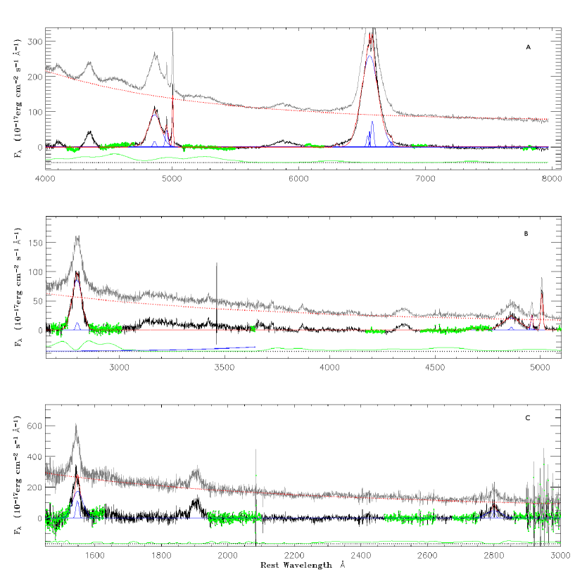
Figure 1: The examples of spectral analysis: (A) low redshift FSRQ SDSS J080131.9+473616.1 ($z=0.157$); (B) middle redshift FSRQ SDSS J074559.3+331334.5 ($z=0.610$); (C) high redshift FSRQ SDSS J081303.8+254211.1 ($z=2.024$). In each panel, the top and middle black lines are the original and the continuum-subtracted spectrum, respectively. The top dotted red line represents the power-law continuum. The middle blue lines are the individual line components in multi-line spectral fitting, and the middle solid red line is integrated lines fitting. The green spectral region in the continuum-subtracted spectrum is used to fit Fe II emission and power-law continuum, and the bottom green line is Fe II emission, which is shifted downwards with arbitrary unit for the sake of presentation. The Balmer continuum is indicated as solid blue lines in the bottom of panel (B), which began at the Balmer edge 3646$\rm\AA$, however, it is not included in the case of (A) and (C) due to the wavelength coverage (see text for details).

The modeling of above three components is performed by minimizing the $\chi^{2}$ in the fitting process. The final multicomponent fit is then subtracted from the observed spectrum. The examples of the fitted power-law, Fe II lines, Balmer continuum and the residual spectra for the sources with low, middle and high redshift are shown in Fig. 1. The Fe II fitting windows are selected as the regions with prominent Fe II line emission while no other strong emission lines, according to Vestergaard & Wilkes (2001) and Kim et al. (2006). The fitting window around the Balmer edge ($3625-3645\rm\AA$) is used to measure the contribution of Balmer continuum, which extends to $\rm Mg~{}II$ line region. The Balmer continuum is not considered when $3625-3645\rm\AA$ is out of the spectrum. Therefore, the inclusion of Balmer continuum depends on the source redshift, which is illustrated in Fig. 1. While the Balmer continuum should be included in the fitting for middle redshift sources, it can be ignored for low and high redshift sources.

The broad emission lines were measured from the continuum subtracted spectra. We mainly focused on several prominent emission lines, i.e. ${\rm Ly\,\alpha},\rm H{\alpha},\rm H{\beta}$, Mg II, C IV. Generally, two gaussian components were adopted to fit each of these lines, indicating the broad and narrow line components, respectively. The blended narrow lines, e.g. [O III] $\lambda\lambda 4959,5007\rm\AA$ and [He II] $\rm\lambda 4686\AA$ blending with $\rm H\beta$, and [S II] $\lambda\lambda 6716,6730\rm\AA$, [N II] $\lambda\lambda 6548,6583\rm\AA$ and [O I]$\rm\lambda 6300\AA$ blending with $\rm H\alpha$, were included as one gaussian component for each line at the fixed line wavelength. The $\chi^{2}$ minimization method was used in fits. The line width FWHM, line flux of broad ${\rm Ly\,\alpha},\rm H{\alpha},\rm H{\beta}$, Mg II and C IV lines were obtained from the final fits for our sample. The examples of the fitting are shown in Fig. 1 for the sources in the different redshift.

3.2 $M_{\rm bh}$ and $L_{\rm BLR}$

There are various empirical relations between the radius of broad line region (BLR) and the continuum luminosity, which can be used to calculate the black hole mass in combination with the line width FWHM of broad emission lines. However, there are defects when using the continuum luminosity to estimate the BLR radius for blazars since the continuum flux of blazars are usually doppler boosted due to the fact that the relativistic jet is oriented close to the line of sight. Alternatively, the broad line emission can be a good indicator of thermal emission from accretion process. Therefore for our FSRQs sample, we estimate the black hole mass by using the empirical relation based on the luminosity and FWHM of broad emission lines. According to the source redshift, we use various relations to estimate the black hole mass: Greene et al. (2005) relation for broad $\rm H\alpha$ line; Vestergaard et al. (2006) for broad $\rm H\beta$ and Kong et al. (2006) for broad Mg II and C IV lines.

Greene & Ho (2005) provided a formula to estimate the black hole mass using the line width and luminosity of broad $\rm H{\alpha}$ alone, which is expressed as

$$M_{\rm BH}(\rm H{\alpha})=(2.0^{+0.4}_{-0.3})\times 10^{6}\Big{(}\frac{{\it L}(\rm H{\alpha})}{10^{42}\,erg\,s^{-1}}\Big{)}^{0.55\pm 0.02}~{}\Big{(}\frac{{\rm FWHM}(\rm H{\alpha})}{10^{3}\,km\,s^{-1}}\Big{)}^{2.06\pm 0.06}{\it M}_{\sun}$$ (3)

For the sources with available FWHM and luminosity of broad $\rm H{\beta}$, the method to calculate $M_{\rm BH}$ is given by Vestergaard & Peterson (2006):

$$M_{\rm BH}(\rm H{\beta})=4.68\times 10^{6}\left(\frac{\it L(\rm H\beta)}{10^{42}\,\rm erg~{}s^{-1}}\right)^{0.63}\left(\frac{\rm FWHM(H\beta)}{1000~{}km~{}s^{-1}}\right)^{2}{\it M}_{\sun}$$ (4)

In addition, Kong et al. (2006) presented the empirical formula to obtain the black hole mass using broad $\rm Mg~{}II$ and $\rm C~{}IV$ for high redshift sources as follows,

$$M_{\rm BH}({\rm Mg~{}II})=2.9\times 10^{6}\left(\frac{L({\rm Mg~{}II})}{\rm 10^{42}\,erg\,s^{-1}}\right)^{0.57\pm 0.12}\left(\frac{\rm FWHM(Mg~{}II)}{\rm 1000\,km\,s^{-1}}\right)^{2}M_{\sun},$$ (5)

$$M_{\rm BH}({\rm C~{}IV})=4.6\times 10^{5}\left(\frac{L({\rm C~{}IV})}{\rm 10^{42}\,erg\,s^{-1}}\right)^{0.60\pm 0.16}\left(\frac{\rm FWHM(C~{}IV)}{\rm 1000\,km\,s^{-1}}\right)^{2}M_{\sun}$$ (6)

In the redshift range of our sample, $M_{\rm BH}$ can be estimated using two of above relations for 122 out of 185 FSRQs. In most sources (113/122), two $M_{\rm BH}$ values are consistent with each other within a factor of three. For low-redshift sources, we first selected the black hole mass estimated from broad $\rm H{\beta}$ line, which is commonly used to estimate the black hole mass for low-redshift sources (e.g. Kaspi et al., 2000; Gu, Cao & Jiang, 2001). In the case that the spectral quality or the spectral fitting of $\rm H{\beta}$ region is poor, we instead use broad $\rm H{\alpha}$ line to estimate the black hole mass. Moreover, we adopted the average value of $M_{\rm BH}~{}({\rm Mg~{}II})$ and $M_{\rm BH}~{}({\rm C~{}IV})$ when both values are available for one source.

In this work, the BLR luminosity $L_{\rm BLR}$ is derived following Celotti, Padovani & Ghisellini (1997) by scaling the strong broad emission lines ${\rm Ly\,\alpha},\rm H{\alpha},\rm H{\beta}$, Mg II and C IV to the quasar template spectrum of Francis et al. (1991), in which Ly$\alpha$ is used as a reference of 100. By adding the contribution of $\rm H\alpha$ with a value of 77, the total relative BLR flux is 555.77, of which $\rm Ly\alpha$ is 100, $\rm H{\alpha}$ 77, $\rm H{\beta}$ 22, $\rm Mg~{}II$ 34, and $\rm C~{}IV$ 63 (Celotti, Padovani & Ghisellini, 1997; Francis et al., 1991). From the BLR luminosity, we estimate the bolometric luminosity as $L_{\rm bol}=10L_{\rm BLR}$ (Netzer, 1990).

4 The thermal emission

In addition to the relativistically beamed, non-thermal jet emission, the thermal emission from the accretion disk and the host galaxy are expected to be present in radio quasars. In some cases, the thermal emission can be dominated over the nonthermal jet emission (e.g. Landt et al., 2008). We estimated the contribution of thermal emission in SEDs as follows (see also Landt et al., 2008), and our sample is thus refined to include only the sources with SEDs dominated by the nonthermal jet emission.

4.1 The accretion disk

Following D’Elia, Padovani & Landt (2003) and Landt et al. (2008), we calculated accretion disk spectra assuming a steady geometrically thin, optically thick accretion disk. In this case the emitted flux is independent of viscosity, and each element of the disk face radiates roughly as a blackbody with a characteristic temperature, which depends only on the mass of the black hole, $M_{\rm BH}$, the accretion rate, $\dot{M}$, and the radius of the innermost stable orbit (e.g., Peterson 1997; Frank et al. 2002). We have adopted the Schwarzschild geometry (nonrotating black hole), and for this the innermost stable orbit is at $r_{\rm in}=6r_{\rm g}$, where $r_{\rm g}$ is the gravitational radius defined as $r_{\rm g}=GM_{\rm BH}/c^{2}$, G is the gravitational constant, and c is the speed of light. Furthermore, we have assumed that the disk is viewed face-on. The accretion disk spectrum is fully constrained by the two quantities, accretion rate and mass of the black hole. We have calculated the accretion rate using the relations $L_{\rm bol}=\epsilon\dot{M}c^{2}$, where $\epsilon$ is the efficiency for converting matter to energy, with $\epsilon\sim 6\%$ in the case of a Schwarzschild black hole. The bolometric luminosity is estimated as $L_{\rm bol}=f^{-1}L_{\rm BLR}$ with $f$ the BLR covering factor, which is not well known, and can be in the range of $\sim 5\%-30\%$ (Maiolino et al. 2001 and references therein). As in Section 3.2, we adopt a canonical value of $f\sim 10\%$ (Peterson 1997). The contribution of accretion disk thermal emission are estimated by calculating the fraction of the thermal emission to the SED data at SDSS optical and $GALEX$ UV region. Tentatively, we simply use a marginal value of 50% at most of SED wavebands to divide the FSRQs into thermal-dominated ($>50\%$) and nonthermal-dominated ($<50\%$), and found that the thermal emission can be dominant in 100/185, 35/185, 2/185 FSRQs for $f=$ 5%, 10%, and 30%, respectively.

4.2 The host galaxy

Usually, the host galaxies of radio quasars are bright ellipticals, and their luminosity only spread in a relatively narrow range (e.g. McLure et al., 2004). We estimated the contribution from host galaxy thermal emission using the elliptical galaxy template of Mannucci et al. (2001), which extends from near-IR to UV frequencies (see also Landt et al., 2008). Slightly different from Landt et al. (2008), we use the bulge absolute luminosity in R-band estimated from $M_{\rm BH}-M_{\rm R}$ relation of McLure et al. (2004) in combination with the estimted black hole mass in Section 3.2,

$$\rm log~{}\it M_{\rm BH}/\rm M_{\odot}=-0.50(\pm 0.02)\it M_{\rm R}\rm-2.74(\pm 0.48)$$ (7)

The contribution of host galaxy thermal emission are estimated by comparing the calculated thermal emission with the SED data at SDSS optical, $GALEX$ UV and 2MASS NIR region. The value of 50% is used to distinguish thermal-dominated with thermal emission $>50\%$ and non-thermal dominated with thermal emission $<50\%$. We found that the thermal emission can be dominant in about 16 of 185 FSRQs.

4.3 Sample refinement

Although the thermal emission may dominate in only small fraction of sources, i.e. accretion disk thermal emission in 35 sources, and host galaxies emission in 16 sources, we combine the contribution of accretion disk and host galaxy to maximize the source number, of which the non-thermal jet emission is not dominated in SED. We simply add the expected thermal emission from accretion disk (using a canonical value $f=10\%$) and host galaxy, then compare with the SED data at SDSS optical, GALEX UV and 2MASS NIR region. Finally, we found the combined thermal emission can dominate over ($>50\%$) nonthermal jet emission in about 67 sources, which are then called thermal-dominated FSRQs in this work and listed in Table 2. The remaining 118 sources are recognized as nonthermal jet-dominated FSRQs in this work (see Table 1).

4.4 $\nu_{\rm peak}$ and $\nu{L{\nu_{\rm peak}}}$

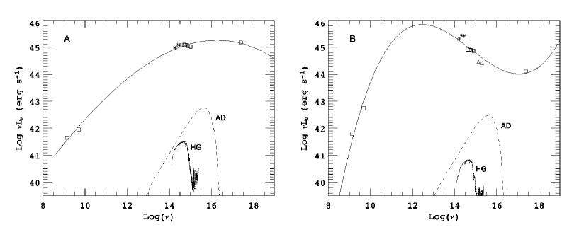
Figure 2: Representative three-degree polynomial fits to the spectral energy distributions of FSRQs in our sample. Open rectangles are data from FIRST, GB6, SDSS and RASS. Stars represent data from 2MASS, and triangles for $GALEX$ UV data. The solid line is the SED fit, while the dotted one (HG) is the calculated emission from host galaxy. The dashed line (AD) is the expected emission from the accretion disk at assuming $f=10\%$ (see text for details). The synchrotron peak frequencies for the two sources are $\nu_{\rm peak}=1.86\times 10^{16}$ Hz (SDSS J150324.7+475830.4, $z=0.345$; A) and $\nu_{\rm peak}=2.88\times 10^{12}$ Hz (SDSS J083148.9+042939.2, $z=0.174$; B). See text for details.

The SED of each quasar was constructed from multi-band data, which covers radio (1.4 and 4.85 GHz), optical (5 - 8 line-free windows selected from SDSS spectra), and X-ray (1keV) data. The optical continuum were picked out with five to eight line-free regions (Forster et al., 2001; Vanden Berk et al., 2001) from the SDSS spectra in the source rest frame, of which no or only very weak Fe lines are present (see Section 3.1). The radio flux at 1.4 and 4.85 GHz are K-corrected to the source rest frame using the spectral index between these two frequencies. The X-ray 1 keV luminosity are obtained after K-correction and correcting the Galactic extinction (Shen et al., 2006). The IR ($J$, $H$, and $K_{s}$) data collected from 2MASS (Skrutskie et al., 2006) were also added to construct SEDs, which are available for 98 FSRQs. Moreover, the Far- (for 117 sources) and near-UV (for 146 sources) data are also added in constructing SEDs, after correcting the Galactic extinction and K-correction using a spectral index of 0.5. Considering the possibility that the X-ray emission of FSRQs can be from the inverse Compton process, we fitted the data points for each source (in a $\rm\nu$ versus $\rm\nu L_{\nu}$ diagram) with a third-degree polynomial following Fossati et al. (1998), which yields an upturn allowing for X-ray data-points that do not lie on the direct extrapolation from the lower energy spectrum (see examples in Fig. 2). Through fitting, we obtained the synchrotron peak frequency and the corresponding peak luminosity for each source. In following analysis, we will present the analysis only for the non-thermal jet-dominated FSRQs (see Table 1).

5 results

5.1 $\alpha_{\rm ro}$ – $\alpha_{\rm ox}$ plane

The broadband properties of our sources can be firstly studied by deriving their $\alpha_{\rm ox}$, $\alpha_{\rm ro}$, and $\alpha_{\rm rx}$ values, which are the usual rest-frame effective spectral indices defined between 5 GHz, 5000 $\rm\AA$, and 1 keV. The 5000 $\rm\AA$ optical continuum flux density is derived (or extrapolated when 5000 $\rm\AA$ is out of the SDSS spectral region) from the direct power-law fit on the 5 - 8 selected line-free SDSS spectral windows in the source rest frame (see Section 3.1). The 5 GHz flux density have been k-corrected using the spectral index between FIRST 1.4 GHz and GB6 4.85 GHz. In Fig. 3, we present $\alpha_{\rm ro}$ - $\alpha_{\rm ox}$ relation for the sample. Following Padovani et al. (2003), three lines are indicated: $\alpha_{\rm rx}=0.85$, typical of 1 Jy FSRQs and LBLs; $\alpha_{\rm rx}=0.78$, the dividing line between HBLs and LBLs; and $\alpha_{\rm rx}=0.70$, typical of RGB BL Lac objects. Moreover, the ‘HBL’ and ‘LBL’ boxes defined in Padovani et al. (2003) are also indicated in the figure, which represent the regions within $2\sigma$ from the mean $\alpha_{\rm ro}$, $\alpha_{\rm ox}$, and $\alpha_{\rm rx}$ values of HBLs and LBLs in the multifrequency AGN catalog of Padovani et al. (1997), respectively (see Fig. 1 in Padovani et al. 2003). This “HBL box” is expected to be populated by high-energy peaked blazars, both BL Lacs and FSRQs. Among total 118 FSRQs, 48 sources have $\alpha_{\rm rx}<0.78$, of which 28 sources locate in HBL box. In contrast, 59 sources among 70 $\alpha_{\rm rx}>0.78$ sources are in LBL box.

5.2 $\nu_{\rm peak}$ and $\nu{L{\nu_{\rm peak}}}$

The relation of the synchrotron peak frequency and peak luminosity is presented in Fig. 4. We found only a weak anti-correlation between the synchrotron peak frequency $\nu_{\rm peak}$ and the peak luminosity $\nu{L{\nu_{\rm peak}}}$ with the Spearman correlation coefficient $r=-0.161$ at $\sim 92\%$ confidence level. The $\nu_{\rm peak}$ distribution ranges $10^{12.4}$ and $10^{16.3}$ Hz for whole sample, and between $10^{13}$ and $10^{15.5}$ Hz for most (111/118) of sources, with $\langle\rm log~{}\nu_{\rm peak}\rangle=14.41\pm 0.74$ Hz for whole sample. We found $\nu_{\rm peak}>10^{15}$ Hz in 25 sources (see Fig. 4), which is larger than the typical value of FSRQs (Fossati et al., 1998). As outliers to blazar sequence, the blue quasars are supposed to have large $\nu_{\rm peak}$ and high $\nu{L{\nu_{\rm peak}}}$ as well (see e.g. Padovani et al., 2003). To further understand the nature of these high $\nu_{\rm peak}$ FSRQs, we combine our sample with the sample of 170 BL Lac objects in Wu, Gu & Jiang (2008). A significant anti-correlation between $\nu_{\rm peak}$ and $\nu{L{\nu_{\rm peak}}}$ is present with the Spearman correlation coefficient $r=-0.343$ at $\gg$ 99.99% confidence level for the combined sample of 288 blazars, which is shown in Fig. 5. This anti-correlation covers about seven order of magnitude in $\nu_{\rm peak}$ for the combined sample. Our FSRQs with high $\nu_{\rm peak}>10^{15}$ Hz have systematically higher peak luminosity than that of BL Lacs, with $\langle\rm log~{}\nu{L{\nu_{\rm peak}}}\rangle=46.41\pm 0.94$ compared to $44.90\pm 0.71$ for BL Lacs at same $\nu_{\rm peak}$ range, and the peak luminosity of some FSRQs are out of the range covered by BL Lacs. However, we found that the thermal emission from accretion disk can be dominated over nonthermal jet emission in 11 of 25 sources with $\nu_{\rm peak}>10^{15}$ Hz if a BLR covering factor of $5\%$ is assumed. Therefore, the possibility that the contribution from the thermal emission causes the high synchrotron peak frequency can not be completely excluded. Although high $\nu_{\rm peak}$ are found in our FSRQs, they do not reach the extreme value of HBLs, which is also found in DXRBS sample when comparing high $\nu_{\rm peak}$ FSRQs with BL Lacs (Padovani et al., 2003). At the lower-left corner of Fig. 5, there are some FSRQs with relatively low synchrotron peak frequency as well as low luminosity, comparable to some low luminosity LBLs. While only a weak anti-correlation present between $\nu_{\rm peak}$ and $\nu{L{\nu_{\rm peak}}}$ for Wu, Gu & Jiang (2008) BL Lacs sample, it becomes significant when combining with our sample. To some extent, this reflects the importance of sample selection in investigating the blazar sequence (e.g. Padovani, 2007). Although the anti-correlation is significant in Fig. 5, we notice that the scatter is significant, mainly caused by the sources in the lower-left corner. However, the extreme sources with high $\nu_{\rm peak}$ as well as high peak luminosity (i.e. at upper-right corner) are still lacking. On the other hand, the large scatter may imply that other parameters may be at work, and the scatter can be much lower once this parameter is included.

We investigate the relationship between $\alpha_{\rm rx}$ and $\nu_{\rm peak}$ for our sample in Fig. 6. A significant anti-correlation is found with a Spearman correlation coefficient $r=-0.443$ at confidence level $\gg 99.99\%$. However, the considerable scatter is also present with the scatter in $\nu_{\rm peak}$ more than one order of magnitude for any given value of $\alpha_{\rm rx}$. The mean $\nu_{\rm peak}$ of FSRQs in HBL box is only slightly larger than that of sources out of the HBL box with a factor of four. Consequently, the FSRQs in HBL box do not exclusively have high $\nu_{\rm peak}$. The $\nu_{\rm peak}$ of souces in HBL box are comparable to those with $\alpha_{\rm rx}<0.78$ but out of HBL box. This actually can be reflected from the relationship between $\alpha_{\rm ro}$ and $\nu_{\rm peak}$ shown in Fig. 7. The significant anti-correlation is found at a confidence level of $\sim 99.9\%$, however the scatter is significant. At any given value of $\alpha_{\rm ro}$, the source could have a low $\nu_{\rm peak}$ or a high $\nu_{\rm peak}$. As a result, the sources out of HBL box with $\alpha_{\rm rx}<0.78$ are not necessary to have lower or higher $\nu_{\rm peak}$ than that of sources in HBL box, though the latter show a wider $\alpha_{\rm ro}$ range. Consistent with the anti-correlation in Fig. 6, the mean $\nu_{\rm peak}$ value of FSRQs with $\alpha_{\rm rx}<0.78$ is larger with a factor of four than that of $\alpha_{\rm rx}>0.78$ sources. Owing to the large scatters in both $\alpha_{\rm rx}-\nu_{\rm peak}$ and $\alpha_{\rm ro}-\nu_{\rm peak}$ relations, it seems that neither solely $\alpha_{\rm rx}$ nor $\alpha_{\rm rx}$ - $\alpha_{\rm rx}$ combination can precisely predict the $\nu_{\rm peak}$ value for our present FSRQs sample.

5.3 ($\nu_{\rm peak}$, $\nu{L{\nu_{\rm peak}}}$) & ($M_{\rm bh}$, $L_{\rm bol}/L_{\rm Edd}$)

The estimation of black hole mass and BLR luminosity (then the corresponding bolometric luminosity) enable us to investigate the relationship between the synchrotron emission and the accretion process. In Figs. 8 and 9, we show the relation of $\nu_{\rm peak}$ & $M_{\rm bh}$, and $\nu_{\rm peak}$ & $L_{\rm bol}/L_{\rm Edd}$, respectively. The black hole mass ranges from $10^{7.4}$ to $10^{10.5}~{}M_{\odot}$ with most of sources ($\sim 86\%$; 102 out of 118 sources) in the range of $10^{8.5}-10^{10}~{}M_{\odot}$, while the eddington ratio $L_{\rm bol}/L_{\rm Edd}$ ranges from $\sim 10^{-2}$ to $\sim 10^{0.6}$, with most of source ($\sim 94\%$; 111 out of 118 sources) in the range of 0.01 to 1. No strong correlations are found either between $\nu_{\rm peak}$ and $M_{\rm bh}$, or between $\nu_{\rm peak}$ & $L_{\rm bol}/L_{\rm Edd}$.

We found a significant correlation between the black hole mass $M_{\rm BH}$ and the synchrotron peak luminosity $\nu{L{\nu_{\rm peak}}}$ with the Spearman correlation coefficient $r=0.724$ at $\sim 99.99\%$ confidence level, which is shown in Fig. 10. Moreover, a significant correlation between $\nu{L{\nu_{\rm peak}}}$ and $L_{\rm bol}/L_{\rm Edd}$ is also found with the Spearman correlation coefficient $r=0.842$ at $\gg$ 99.99% confidence level (see Fig. 11). Both correlations still present when we perform the Spearman partial correlation analysis to exclude the common dependence on redshift. The ordinary least-square (OLS) bisector linear fit to $\nu{L{\nu_{\rm peak}}}$ and $L_{\rm bol}/L_{\rm Edd}$ gives,

$$\rm log~{}\it\nu{L{\nu_{\rm peak}}}=\rm(1.73\pm 0.11)~{}\rm log~{}\it L_{\rm bol}/L_{\rm Edd}+\rm(47.92\pm 0.11)$$ (8)

This result indicates that the jet physics may be tightly related with the accretion process.

We plot the ratio of BLR luminosity to synchrotron peak luminosity $L_{\rm BLR}/\nu{L{\nu_{\rm peak}}}$ and synchrotron peak frequency $\rm\nu_{\rm peak}$ in Fig. 12, from which a significant correlation between these two parameters is found with the Spearman correlation coefficient $r=0.480$ at $\gg$ 99.99% confidence level. However, there is no strong correlation between the synchrotron peak frequency and BLR luminosity.

The jet-disk relation can be further explored through the relationship between $\nu{L{\nu_{\rm peak}}}$ and $L_{\rm BLR}$ shown in Fig. 13. A significant correlation is present with a Spearman correlation coefficient of $r=0.909$ at confidence level $\gg 99.99\%$, which remains in partial correlation analysis to exclude the common dependence on redshift. The ordinary least-square (OLS) bisector linear fit gives,

$$\rm log~{}\it\nu{L{\nu_{\rm peak}}}=\rm(0.95\pm 0.06)~{}\rm log~{}\it L_{\rm BLR}+\rm(3.14\pm 2.84)$$ (9)

Our result implies a tight relation between jet and disk, which is consistent with previous findings in various occasions, from the strong correlations either between the radio emission and emission line luminosity (e.g. Rawlings et al. 1989; Cao & Jiang 2001), or between the emission line luminosity and jet kinetic power in different scales (Rawlings & Saunders 1991; Celotti & Fabian 1993; Wang et al. 2004; Gu, Cao & Jiang 2009). Moreover, our result is consistent with the nearly proportional relation, $Q\propto L_{\rm NLR}^{0.9\pm 0.2}$, found between the jet bulk kinetic power and narrow line luminosity (Rawlings & Saunders 1991). However, it should be noted that the synchrotron peak luminosity of blazars are usually Doppler boosted, therefore, it may not be a good indicator of jet power. It would be necessary to improve our result using intrinsic parameters, either the intrinsic synchrotron peak luminosity after eliminating the beaming effect, or the jet power.

6 discussion

According to the blazar sequence, FSRQs with high synchrotron peak frequency, e.g. $\nu_{\rm peak}>10^{15}$ Hz, and X-rays dominated by synchrotron emission are not expected to exist. Due to its importance, such objects have been extensively searched (see Padovani, 2007, and references therein). The discoveries of such blazars have been claimed, however, mainly on the basis of their broad spectral indices, i.e. the ratios of radio/optical/X-ray fluxes (Padovani et al., 2002; Bassani et al., 2007; Giommi et al., 2007). In this sense, the X-ray spectroscopy is required to confirm the nature of the X-ray emission in these blazars. In its simplest form, a X-ray spectral index of $\alpha<1$ indicates a inverse Compton origin, while $\alpha>1$ for synchrotron X-ray emission. Maraschi et al. (2008) investigate the X-ray spectra for a sample of 10 X-ray selected FSRQs from the Einstein Medium Sensitivity Survey (EMSS) and four controversial sources claimed to have synchrotron X-ray emission. They found that, in the case of the EMSS broad line blazars, X-ray selection does not lead to find sources with synchrotron peaks in the UV/X-ray range, as was the case for X-ray-selected BL Lacs. Instead, for a wide range of radio powers all the sources with broad emission lines show similar SEDs, with synchrotron components peaking below the optical/UV range. Moreover, the authors argued that four ‘anomalous’ blazars are no longer ‘anomalous’ after a complete analysis of $Swift$ and $INTEGRAL$ data, with two sources having inverse Compton X-rays, one source being HBL, and the remaining one being narrow line Seyfert 1 galaxy without unambiguous evidence of X-ray emission from a relativistic jet. Similarly, the $XMM-Newton$ and $Chandra$ X-ray spectroscopy of 10 FSRQs were investigated by Landt et al. (2008), which are candidates to have an X-ray spectrum dominated by jet synchrotron emission. However, the authors failed to find FSRQs with X-ray spectra dominated by jet synchrotron emission, instead, the X-rays are either from inverse Compton or are at transition between the synchrotron and inverse Compton jet components as in IBLs. So, despite the efforts to search for objects which may violate the sequence trends no strong outliers have been found (Maraschi et al. 2008). As a severe challenge to blazar sequence, the selection of important candidates of high $\nu_{\rm peak}$ luminous FSRQs are refined to choose highly core-dominated radio quasars with low radio core to X-ray luminosity ratios, e.g. log $(L_{\rm core}/L_{\rm X})\lesssim 5$ (Landt et al., 2008). The inverse Compton emission is expected to peak at $\gamma$-ray frequencies, therefore, the high energy-peaked FSRQs could be prime targets for the Fermi Gamma-ray Telescope (Landt et al., 2008). Although the high energy-peaked FSRQs are not firmly found yet, Ghisellini & Tavecchio (2008) proposed a model to explain the existence of blue quasars. In their scenario, the jet dissipation region is out of the broad line region, resulting in a much reduced energy density of BLR photons in jet region. Therefore, the cooling due to the inverse Compton process is not severe, causing a high synchrotron peak frequency though the source luminosity is high.

Although the anti-correlation between $\nu_{\rm peak}$ and $\nu{L{\nu_{\rm peak}}}$ for the combined sample of 288 blazars (Fig. 5) is significant, it largely differs with the blazar sequence in its significant scatter, which indicates that the synchrotron peak luminosity can not explicitly determine the synchrotron peak frequency, and vice verse. The advantages of using the synchrotron peak luminosity is that the most of synchrotron emission are radiated at synchrotron peak frequency, at which the luminosity can be a good indicator of synchrotron emission. Since the synchrotron peak frequency varies from source to source, the luminosity at fixed wavebands (e.g. optical) is actually from the different portion of source SED. The defect of the synchrotron peak luminosity lies in the contamination from beaming effect, which precludes it to well indicate the intrinsic source power. Only when the Doppler boosting is known for each source, the intrinsic source power can be obtained. This can not be performed at present stage. However, this effect has been explored through eliminating the Doppler boosting in blazar samples. Interestingly, recent studies have shown that the negative correlation between $\nu_{\rm peak}$ and $\nu{L{\nu_{\rm peak}}}$ is likely an artefact of Doppler boosting (Nieppola et al., 2008; Wu, Gu & Jiang, 2008). According to these authors, the negative correlation is not present when the intrinsic parameters are used, conversely, a positive correlation is claimed. The key point in these studies is the strong anti-correlation between the Doppler factor and synchrotron peak frequency in the way that the sources with their synchrotron peak at low energies are significantly more boosted than high $\nu_{\rm peak}$ sources, which is found either from the variability Doppler factor (Nieppola et al., 2008) or from the one estimated with empirical relation (Wu, Gu & Jiang, 2008).

The synchrotron peak frequency $\nu_{\rm peak}\propto B\delta\gamma_{\rm peak}^{2}$, where $B$ is the magnetic field, $\delta$ the Doppler factor, and $\gamma_{\rm peak}$ a characteristic electron energy that is determined by a competition between accelerating and cooling processes. Different from BL Lacs, the external inverse Compton scattering is thought to be the dominant cooling process in FSRQs, especially that upon BLR photons. Through model fitting to blazar SEDs, the electron peak energy is found to be well anti-correlated with the total energy density (radiative and magnetic), which is thought to be the physics behind the phenomenological blazar sequence (Ghisellini et al., 1998; Ghisellini, Celotti & Costamante, 2002; Celotti & Ghisellini, 2008). More energy density inside the jet cause a more severe cooling, resulting in a smaller $\gamma_{\rm peak}$ then $\nu_{\rm peak}$. According to the equations we used to estimate the black hole mass, we have the BLR radius approximately with $R_{\rm BLR}\propto L_{\rm BLR}^{0.6}$ for $\rm H\alpha,H\beta,MgII,CIV$ broad lines. Consequently, the energy density of BLR photons $u_{\rm BLR}^{*}$ is expected to be proportional to $L_{\rm BLR}^{-0.2}$. We expect to see an anti-correlation between $\nu_{\rm peak}$ and the BLR luminosity $L_{\rm BLR}$. However, we failed to find any correlation between $\nu_{\rm peak}$ and $L_{\rm BLR}$. Several factors may erase the expected anti-correlation, e.g. the scatters in the derivation of BLR luminosity from individual lines, the accuracy of empirical relation in estimating BLR radius, and the inclusion of $B$ and $\delta$ (vary from source to source) in $\nu_{\rm peak}$. As a result, the positive correlation between $\nu_{\rm peak}$ and $L_{\rm BLR}/\nu{L{\nu_{\rm peak}}}$ can be partly (if not all) the result of the weak anti-correlation between $\nu_{\rm peak}$ and $\nu{L{\nu_{\rm peak}}}$ (see Fig. 12). Nevertheless, it indicates that FSRQs with higher ratio of disk to jet emission could have higher peak frequency.

The FSRQs in our sample are defined from the flat spectrum between 1.4 and 4.85 GHz $\alpha<0.5$. However, this definition may influenced by several factors. It is well known that FSRQs usually show strong and rapid variability (e.g. Gu et al., 2006). Another factor is the different resolution at 1.4 and 4.85 GHz. FIRST 1.4 GHz data are obtained from VLA observations, which have much higher resolution than Green Bank telescope observations for 4.85 GHz data. In these respects, the simultaneous multi-band observations with same telescope configuration (same resolution) is required to calculate the radio spectral index, and then to understand the nature of sources.

7 Summary

We have constructed a sample of 185 Flat Spectrum Radio Quasars (FSRQs) by cross-correlating the Shen et al. (2006) SDSS DR3 X-ray quasar sample with FIRST and GB6 radio catalogues. From the spectrum energy distraction (SED) constructed using multi-band (radio, optical, Infrared and X-ray) data, we derived the synchrotron peak frequency and peak luminosity. The black hole mass $M_{\rm BH}$ and the broad line region (BLR) luminosity (then the bolometric luminosity $L_{\rm bol}$) were obtained by measuring the line-width and strength of broad emission lines from SDSS spectra. We define a subsample of 118 FSRQs, of which the nonthermal jet emission are thought to be dominated over thermal ones from accretion disk and host galaxy. The various correlations were explored for this subsample. The main results are summarized below.

1. A weak anti-correlation is found between the synchrotron peak frequency and peak luminosity. When combining our FSRQs sample with the Wu, Gu & Jiang (2008) sample of 170 BL Lac objects, a significant anti-correlation between the synchrotron peak frequency and luminosity apparently presents covering about seven order of magnitude in $\nu_{\rm peak}$. However, the anti-correlation differs with the blazar sequence in the large scatter.

2. We found 25 FSRQs having synchrotron peak frequency $\nu_{\rm peak}>10^{15}$ Hz, which is higher than the typical value for FSRQs. These sources with high $\nu_{\rm peak}$ could be the targets for the Fermi Gamma-ray telescope. At similar peak frequency, the peak luminosity of FSRQs with $\nu_{\rm peak}>10^{15}$ Hz is systematically higher than that of BL Lac objects, with some FSRQs out of the range covered by BL Lac objects. Though high $\nu_{\rm peak}$ are found in some FSRQs, they do not reach the extreme value of BL Lacs.

3. No strong correlations are found either between the synchrotron peak frequency and black hole mass, or between the synchrotron peak frequency and the Eddington ratio. The peak luminosity is found to be tightly correlated with both black hole mass and the Eddington ratio indicating that the jet physics may be tightly related with the accretion process, which is further confirmed by the tight correlation between the synchrotron peak luminosity and the BLR luminosity.

8 acknowledgements

We thank the referee, Hermine Landt, for insightful suggestions, which is great helpful in improving our paper. We thank Tinggui Wang, Xiaobo Dong, Dawei Xu, Wei Zhang, Tuo Ji and Chen Hu for helps on data reduction. Z.Y. Chen thanks Center for Astrophysics of USTC for hospitality during his stay in USTC. Shiyin Shen are appreciated for providing the X-ray data, Marianne Vestergaard for Fe templates, and Paolo Padovani for information on ‘HBL box’. We thank Markus Böttcher, Dongrong Jiang, Zhonghui Fan and Fuguo Xie for useful discussions. This work makes use of data products from the Two Micron All Sky Survey, which is a joint project of the University of Massachusetts and the Infrared Processing and Analysis Center/California Institute of Technology, funded by the National Aeronautics and Space Administration and the National Science Foundation. This work is supported by National Science Foundation of China (grants 10633010, 10703009, 10833002, 10773020 and 10821302), 973 Program (No. 2009CB824800), and the CAS (KJCX2-YW-T03).

Funding for the SDSS and SDSS-II has been provided by the Alfred P. Sloan Foundation, the Participating Institutions, the National Science Foundation, the U.S. Department of Energy, the National Aeronautics and Space Administration, the Japanese Monbukagakusho, the Max Planck Society, and the Higher Education Funding Council for England. The SDSS Web Site is http://www.sdss.org/.

The SDSS is managed by the Astrophysical Research Consortium for the Participating Institutions. The Participating Institutions are the American Museum of Natural History, Astrophysical Institute Potsdam, University of Basel, University of Cambridge, Case Western Reserve University, University of Chicago, Drexel University, Fermilab, the Institute for Advanced Study, the Japan Participation Group, Johns Hopkins University, the Joint Institute for Nuclear Astrophysics, the Kavli Institute for Particle Astrophysics and Cosmology, the Korean Scientist Group, the Chinese Academy of Sciences (LAMOST), Los Alamos National Laboratory, the Max-Planck-Institute for Astronomy (MPIA), the Max-Planck-Institute for Astrophysics (MPA), New Mexico State University, Ohio State University, University of Pittsburgh, University of Portsmouth, Princeton University, the United States Naval Observatory, and the University of Washington.

Table 1: Nonthermal jet-dominated FSRQs. (1) Source SDSS name; (2) redshift; (3) black hole mass; (4) synchrotron peak luminosity; (5)broad line region luminosity; (6) bolometric luminosity; (7) synchrotron peak frequency; spectral indices between the rest-frame frequencies of (8) 5 GHz and 5000 $\rm\AA$, (9) 5000 $\rm\AA$ and 1 keV, (10) 5 GHz and 1 keV.

SDSS name	$z$	${\rm Log}~{}M_{\rm BH}$	${\rm Log}~{}\nu L_{\nu{\rm peak}}$	${\rm Log}~{}L_{\rm BLR}$	${\rm Log}~{}L_{\rm bol}$	${\rm Log}~{}\nu_{\rm peak}$	$\alpha_{\rm ro}$	$\alpha_{\rm ox}$	$\alpha_{\rm rx}$
		($M_{\odot}$)	($\rm erg\,s^{-1}$)	($\rm erg\,s^{-1}$)	($\rm erg\,s^{-1}$)	(Hz)
(1)	(2)	(3)	(4)	(5)	(6)	(7)	(8)	(9)	(10)
J001130.4+005752.1	1.492	8.36	46.18	45.28	46.28	14.95	0.555	1.306	0.809
J013352.7+011343.6	0.308	8.56	44.75	43.88	44.88	14.41	0.475	1.288	0.750
J074541.7+314256.6	0.461	9.66	46.14	45.64	46.64	14.93	0.521	1.666	0.909
J074625.9+254902.2	2.979	9.69	47.42	46.62	47.62	14.55	0.574	1.389	0.850
J081009.9+384756.9	3.946	9.33	47.76	47.08	48.08	15.12	0.050	1.882	0.671
J081303.8+254211.1	2.024	9.68	47.30	46.10	47.10	13.44	0.508	1.377	0.802
J082455.5+391641.8	1.216	8.71	46.81	45.30	46.30	13.64	0.599	1.539	0.918
J083148.9+042939.2	0.174	7.42	45.86	42.58	43.58	12.46	0.602	1.303	0.840
J083636.9+412554.9	1.301	9.29	46.78	45.87	46.87	15.52	0.473	1.183	0.714
J085220.5+473458.4	2.420	9.25	46.83	45.92	46.92	15.30	0.517	1.108	0.718
J085442.0+575730.1	1.317	9.59	46.99	46.11	47.11	13.16	0.590	1.475	0.890
J090304.0+465104.5	1.470	9.47	46.68	45.95	46.95	14.30	0.622	1.497	0.919
J090910.1+012136.0	1.024	9.33	46.72	45.78	46.78	13.98	0.515	1.517	0.855
J092058.5+444153.9	2.190	9.84	47.99	46.72	47.72	12.88	0.446	1.502	0.804
J092656.7+041613.0	1.036	10.14	46.45	45.96	46.96	14.55	0.300	1.242	0.619
J093035.1+464408.6	2.033	9.38	47.13	46.00	47.00	14.99	0.420	1.540	0.800
J093200.1+553347.0	0.266	8.92	44.87	43.95	44.95	14.22	0.420	1.514	0.791
J093256.8+074211.9	1.004	9.23	46.15	45.51	46.51	14.41	0.285	1.479	0.690
J093309.3+461534.6	0.778	9.39	45.73	45.03	46.03	15.33	0.414	1.303	0.715
J094855.4+403944.7	1.249	9.39	46.60	45.86	46.86	14.34	0.608	1.513	0.915
J094857.3+002225.6	0.585	8.41	45.43	44.32	45.32	14.38	0.609	1.343	0.858
J095556.4+061642.5	1.278	9.54	46.98	45.86	46.86	13.17	0.334	1.428	0.705
J095738.2+552257.9	0.895	9.11	46.52	45.07	46.07	13.23	0.669	1.532	0.961
J095819.7+472507.7	1.882	9.52	47.14	46.16	47.16	13.72	0.590	1.451	0.882
J095855.1+423703.8	0.664	8.80	45.39	44.72	45.72	14.79	0.553	1.189	0.769
J100556.0+433238.5	1.587	8.94	46.29	45.36	46.36	13.29	0.521	1.366	0.808
J101027.5+413238.9	0.612	9.56	46.10	45.56	46.56	14.68	0.570	1.376	0.843
J101122.6+470042.2	2.928	9.46	47.52	46.19	47.19	15.21	0.249	1.506	0.675
J101557.1+010913.7	0.780	9.85	46.36	45.79	46.79	14.95	0.449	1.740	0.887
J101725.9+611627.5	2.805	10.17	47.77	46.76	47.76	14.51	0.468	1.558	0.837
J102235.6+454105.4	0.743	8.63	45.06	44.21	45.21	13.20	0.564	1.318	0.819
J102429.0+052952.4	1.482	9.65	46.98	46.05	47.05	13.47	0.251	1.694	0.740
J102713.1+480313.5	1.286	9.23	46.31	45.37	46.37	13.54	0.570	1.385	0.846
J103025.0+551622.3	0.434	8.81	45.50	44.89	45.89	14.98	0.387	1.560	0.785
J103050.9+531028.5	1.197	9.41	46.48	45.86	46.86	14.25	0.216	1.487	0.647
J103144.7+602030.7	1.230	9.21	46.43	45.57	46.57	13.96	0.495	1.462	0.823
J103351.4+605107.5	1.401	9.15	46.65	45.20	46.20	13.59	0.546	1.573	0.894
J104146.8+523328.4	0.678	9.53	46.07	45.54	46.54	15.21	0.576	1.492	0.886
J104148.9+523355.6	2.301	9.49	48.33	46.87	47.87	13.10	0.336	1.688	0.794
J104410.6+532220.6	1.901	9.44	47.12	45.96	46.96	13.84	0.477	1.512	0.828
J104542.2+525112.6	1.058	9.33	46.30	45.64	46.64	14.19	0.409	1.496	0.777
J104552.7+062436.3	1.509	10.02	47.38	46.30	47.30	13.46	0.424	1.719	0.863
J104732.3+483531.3	0.866	8.93	45.60	44.99	45.99	14.84	0.508	1.361	0.797
J105654.2+051713.2	0.456	8.94	45.15	44.55	45.55	15.07	0.484	1.326	0.770
J111914.3+600457.2	2.646	10.43	48.14	47.20	48.20	15.24	0.275	1.459	0.677
J112115.7+575446.8	1.274	9.24	46.34	45.55	46.55	14.08	0.293	1.383	0.663
J113245.6+003427.7	1.223	9.09	47.46	45.04	46.04	13.09	0.384	1.836	0.876
J114521.3+045526.7	1.343	9.37	46.20	45.58	46.58	14.40	0.596	1.428	0.878
J120127.4+090040.4	1.016	9.90	46.69	46.13	47.13	14.68	0.233	1.365	0.617
J121201.6+605034.6	1.146	9.38	46.25	45.66	46.66	14.35	0.314	1.490	0.713
J121347.5+000130.1	0.962	9.40	46.18	45.65	46.65	15.04	0.434	1.373	0.752
J122106.9+454852.2	0.525	9.26	45.62	45.06	46.06	15.59	0.429	1.234	0.702
J122339.3+461118.7	1.013	9.26	46.33	45.59	46.59	13.83	0.521	1.367	0.808
J122452.4+033050.3	0.956	9.24	46.03	45.47	46.47	13.30	0.770	1.374	0.975
J123530.6+522828.0	1.651	9.70	47.00	46.05	47.05	14.00	0.317	1.590	0.749
J123932.8+044305.4	1.762	9.18	46.31	45.67	46.67	13.94	0.627	1.165	0.809
J125500.5+034043.2	0.437	8.86	45.29	44.48	45.48	15.96	0.524	0.998	0.685
J125545.1+612450.8	2.056	9.56	46.70	45.93	46.93	13.84	0.439	1.251	0.714
J130217.2+481917.5	0.874	9.09	46.07	45.50	46.50	14.11	0.556	1.320	0.815
J130603.4+552943.7	1.601	9.53	46.90	46.25	47.25	14.38	0.473	1.489	0.818

Table 1: Continued…

SDSS name	$z$	${\rm Log}~{}M_{\rm BH}$	${\rm Log}~{}\nu L_{\nu{\rm peak}}$	${\rm Log}~{}L_{\rm BLR}$	${\rm Log}~{}L_{\rm bol}$	${\rm Log}~{}\nu_{\rm peak}$	$\alpha_{\rm ro}$	$\alpha_{\rm ox}$	$\alpha_{\rm rx}$
		($M_{\odot}$)	($\rm erg\,s^{-1}$)	($\rm erg\,s^{-1}$)	($\rm erg\,s^{-1}$)	(Hz)
(1)	(2)	(3)	(4)	(5)	(6)	(7)	(8)	(9)	(10)
J130909.8+555738.5	1.629	9.64	47.06	46.31	47.31	14.80	0.450	1.665	0.861
J133245.3+472222.6	0.669	8.62	45.70	44.59	45.59	13.69	0.591	1.441	0.879
J133437.4+563147.9	0.343	8.11	44.51	43.67	44.67	14.32	0.584	1.403	0.862
J133749.6+550102.3	1.099	9.00	46.38	45.48	46.48	14.33	0.565	1.640	0.930
J133802.8+423957.2	2.237	9.56	47.27	46.70	47.70	15.22	0.241	1.393	0.632
J134357.6+575442.6	0.933	8.93	45.77	45.13	46.13	14.70	0.598	1.346	0.852
J134934.7+534116.8	0.979	9.65	46.35	45.81	46.81	15.03	0.617	1.437	0.895
J135054.6+052206.6	0.442	9.30	45.27	44.70	45.70	14.64	0.457	1.470	0.800
J135351.6+015153.3	1.608	9.45	46.64	46.22	47.22	14.56	0.509	1.454	0.829
J135726.4+001543.8	0.662	9.11	45.45	45.10	46.10	14.86	0.579	1.271	0.813
J135817.6+575204.4	1.373	9.72	47.29	46.38	47.38	13.92	0.210	1.693	0.713
J140126.2+520834.6	2.972	9.69	47.86	47.19	48.19	15.01	0.219	1.626	0.696
J141159.7+423950.4	0.886	9.60	46.25	45.72	46.72	14.85	0.382	1.629	0.805
J141324.2+530525.7	0.456	8.10	44.57	43.55	44.55	13.34	0.626	1.289	0.851
J141708.2+460705.6	1.559	9.68	47.02	46.43	47.43	14.84	0.534	1.655	0.914
J142020.7+462441.0	1.245	9.50	45.94	45.30	46.30	15.27	0.385	1.370	0.719
J145247.4+473529.1	1.158	9.48	46.08	45.62	46.62	14.88	0.279	1.288	0.621
J145859.4+041614.1	0.392	8.20	45.35	43.28	44.28	12.76	0.669	1.502	0.951
J150031.8+483646.8	1.028	9.86	46.87	46.31	47.31	15.47	0.121	1.188	0.483
J150324.7+475830.4	0.345	7.49	45.28	42.87	43.87	16.27	0.400	0.965	0.591
J150759.7+041512.1	1.701	9.61	47.33	46.21	47.21	14.54	0.303	1.848	0.827
J152544.7+354446.7	1.101	9.16	45.96	45.32	46.32	13.93	0.356	1.394	0.708
J153107.4+584410.0	1.724	10.00	47.20	46.61	47.61	14.36	0.265	1.759	0.771
J153232.3+513001.5	1.876	9.68	47.10	46.42	47.42	14.30	0.329	1.726	0.803
J153404.8+482340.7	0.543	8.52	45.17	44.43	45.43	14.73	0.605	1.408	0.877
J153432.6+492049.2	1.294	9.41	46.49	45.76	46.76	13.85	0.414	1.561	0.803
J153457.2+583923.5	1.901	9.28	47.04	46.43	47.43	14.71	0.368	1.301	0.684
J154502.8+513500.9	1.930	10.05	47.39	46.54	47.54	15.35	0.483	1.447	0.810
J154917.4+503805.9	2.175	9.84	47.38	46.56	47.56	13.61	0.561	1.277	0.804
J154929.4+023701.1	0.414	8.95	45.40	44.98	45.98	14.75	0.667	1.576	0.975
J160226.9+274141.6	0.938	9.45	46.09	45.63	46.63	14.48	0.481	1.425	0.801
J160623.6+540555.7	0.876	9.40	46.12	45.51	46.51	15.36	0.483	1.264	0.748
J160658.3+271705.9	0.934	9.01	45.77	45.38	46.38	15.16	0.627	1.311	0.859
J160822.1+401217.9	0.628	8.33	45.14	44.08	45.08	13.49	0.655	1.322	0.881
J160913.2+535429.7	0.992	9.72	46.16	45.54	46.54	14.52	0.471	1.346	0.768
J161447.0+374607.3	1.532	9.77	47.43	46.40	47.40	14.55	0.183	1.992	0.796
J162229.3+400643.5	0.688	9.04	45.49	44.90	45.90	14.51	0.519	1.267	0.773
J162307.6+390932.5	1.975	9.90	47.72	46.76	47.76	14.45	0.336	1.824	0.841
J162330.6+355933.1	0.866	9.32	45.85	45.32	46.32	14.50	0.574	1.478	0.881
J162422.0+392441.0	1.116	9.13	46.26	45.58	46.58	14.84	0.438	1.348	0.746
J162553.3+434713.8	1.048	8.79	46.08	45.30	46.30	14.81	0.466	1.227	0.724
J162901.3+400759.6	0.272	8.06	44.71	43.51	44.51	15.35	0.363	1.405	0.716
J163302.1+392427.6	1.024	9.51	46.68	46.01	47.01	14.87	0.258	1.757	0.766
J163515.5+380804.6	1.814	9.83	47.55	46.36	47.36	13.79	0.582	1.861	1.016
J163709.3+414030.6	0.760	10.05	46.06	45.75	46.75	14.84	0.299	1.527	0.715
J163755.2+250930.5	1.107	9.50	46.42	45.63	46.63	14.73	0.295	1.460	0.690
J164258.8+394837.2	0.593	9.21	46.75	45.30	46.30	13.33	0.656	1.897	1.077
J164829.2+410405.9	0.852	9.38	45.62	45.10	46.10	14.15	0.618	1.222	0.823
J165005.5+414032.6	0.585	9.05	45.56	45.03	46.03	15.31	0.529	1.296	0.789
J165201.5+623209.3	1.633	9.00	46.57	45.55	46.55	14.01	0.394	1.468	0.758
J165329.9+310756.9	1.298	9.55	46.71	46.16	47.16	15.04	0.406	1.588	0.806
J165931.9+373529.0	0.771	9.59	45.94	45.46	46.46	15.23	0.371	1.467	0.742
J170232.6+315752.2	1.951	9.89	47.38	46.44	47.44	15.36	0.229	1.542	0.674
J170425.1+333146.1	0.290	8.30	44.68	43.68	44.68	14.71	0.372	1.431	0.731
J170648.1+321422.7	1.070	9.69	46.78	46.15	47.15	14.86	0.231	1.478	0.654
J171715.2+262149.1	1.934	9.88	46.98	46.36	47.36	14.70	0.357	1.510	0.748
J172732.4+584634.1	0.844	9.03	45.62	45.11	46.11	14.97	0.579	1.343	0.838
J213638.6+004154.5	1.941	9.92	48.22	46.83	47.83	13.12	0.610	1.728	0.989

Table 2: Thermal-dominated FSRQs. (1) Source SDSS name; (2) redshift; (3) black hole mass; (4) synchrotron peak luminosity; (5)broad line region luminosity; (6) bolometric luminosity; (7) synchrotron peak frequency; spectral indices between the rest-frame frequencies of (8) 5 GHz and 5000 $\rm\AA$, (9) 5000 $\rm\AA$ and 1 keV, (10) 5 GHz and 1 keV.

SDSS name	$z$	${\rm Log}~{}M_{\rm BH}$	${\rm Log}~{}\nu L_{\nu{\rm peak}}$	${\rm Log}~{}L_{\rm BLR}$	${\rm Log}~{}L_{\rm bol}$	${\rm Log}~{}\nu_{\rm peak}$	$\alpha_{\rm ro}$	$\alpha_{\rm ox}$	$\alpha_{\rm rx}$
		($M_{\odot}$)	($\rm erg\,s^{-1}$)	($\rm erg\,s^{-1}$)	($\rm erg\,s^{-1}$)	(Hz)
(1)	(2)	(3)	(4)	(5)	(6)	(7)	(8)	(9)	(10)
J021225.6+010056.1	0.513	9.19	45.31	44.73	45.73	15.77	0.468	1.111	0.686
J074218.2+194719.7	0.657	9.71	45.84	45.49	46.49	15.22	0.395	1.498	0.769
J074242.2+374402.1	0.806	9.51	45.67	45.30	46.30	13.67	0.467	1.117	0.688
J074559.3+331334.5	0.610	9.26	45.42	45.06	46.06	14.30	0.569	1.401	0.851
J075448.8+303355.1	0.795	9.74	46.04	45.58	46.58	14.64	0.467	1.239	0.728
J080131.9+473616.1	0.157	8.96	44.93	44.17	45.17	15.23	0.353	1.541	0.756
J080644.4+484149.1	0.370	9.31	45.15	44.18	45.18	14.47	0.584	1.443	0.876
J080856.6+405244.9	1.418	9.38	46.59	45.93	46.93	13.05	0.622	1.313	0.856
J081059.0+413402.6	0.507	8.74	45.47	44.56	45.56	13.16	0.614	1.420	0.887
J081409.2+323731.9	0.844	9.37	45.67	45.32	46.32	14.71	0.618	1.120	0.788
J081916.5+264203.2	0.526	8.89	45.02	44.48	45.48	15.12	0.582	1.277	0.817
J083353.9+422401.8	0.249	7.05	45.03	42.94	43.94	13.73	0.568	1.501	0.884
J084203.7+401831.4	0.152	8.66	44.44	43.76	44.76	14.77	0.379	1.532	0.770
J084650.0+064148.9	0.616	9.69	45.77	45.31	46.31	15.18	0.463	1.360	0.767
J085040.0+543753.2	0.367	9.58	45.01	44.02	45.02	13.23	0.495	1.434	0.813
J090835.8+415046.0	0.734	9.05	45.49	44.95	45.95	14.49	0.637	1.284	0.856
J091401.8+050750.6	0.301	9.81	45.08	44.32	45.32	14.16	0.535	1.572	0.886
J092554.7+400414.2	0.471	9.53	45.38	44.88	45.88	14.95	0.356	1.421	0.717
J092703.0+390220.7	0.695	9.68	46.42	45.62	46.62	13.22	0.775	1.531	1.031
J093712.3+500852.0	0.276	9.18	44.92	43.04	44.04	13.06	0.604	1.229	0.816
J100017.6+000523.9	0.905	9.31	46.03	45.69	46.69	13.30	0.717	1.186	0.876
J102106.0+452331.6	0.364	9.15	44.77	44.04	45.04	15.17	0.533	1.307	0.795
J102738.5+605016.7	0.332	9.80	44.98	44.03	45.03	14.93	0.356	1.254	0.660
J103214.6+635950.2	0.556	9.18	45.06	44.55	45.55	14.78	0.448	1.362	0.758
J104207.6+501322.1	1.265	9.46	47.60	45.34	46.34	12.48	0.288	1.534	0.710
J110539.0+020257.2	0.105	8.01	44.26	43.44	44.44	13.55	0.539	1.551	0.882
J110718.9+100418.1	0.633	9.38	45.35	44.88	45.88	13.53	0.564	1.250	0.797
J112023.2+540426.9	0.923	9.09	45.63	45.29	46.29	15.89	0.666	0.907	0.748
J113251.1+541031.6	1.624	9.66	46.42	46.21	47.21	14.59	0.498	1.196	0.735
J114803.2+565411.4	0.451	9.14	45.21	44.85	45.85	15.18	0.463	1.388	0.776
J115542.5+021411.3	0.873	9.59	46.02	45.54	46.54	14.40	0.520	1.494	0.850
J120822.5+524013.5	0.432	9.25	45.34	44.93	45.93	14.85	0.370	1.551	0.770
J122940.9+624255.0	0.967	9.56	46.05	45.45	46.45	14.09	0.414	1.430	0.759
J123157.1+542028.8	0.516	9.27	44.80	44.53	45.53	14.93	0.506	1.228	0.751
J123807.8+532555.8	0.347	9.88	45.03	44.40	45.40	14.97	0.449	1.479	0.799
J124116.5+514130.1	0.823	9.79	46.05	45.58	46.58	13.77	0.490	1.278	0.757
J124139.7+493405.6	0.474	9.36	45.43	44.85	45.85	14.53	0.404	1.352	0.725
J130444.0+013230.9	2.288	9.06	46.50	46.13	47.13	13.77	0.422	1.229	0.696
J130554.2+014929.9	0.733	9.91	45.96	45.39	46.39	14.66	0.490	1.572	0.856
J131211.1+480925.2	0.715	9.86	45.92	45.48	46.48	15.15	0.462	1.484	0.808
J131827.1+620036.2	0.307	8.37	44.74	43.76	44.76	13.55	0.545	1.369	0.824
J132631.5+473755.8	0.682	9.26	45.45	44.93	45.93	13.63	0.516	1.305	0.784
J133253.3+020045.4	0.216	8.14	45.12	43.31	44.31	12.42	0.760	1.335	0.955
J134617.6+622044.7	0.117	8.16	44.34	43.34	44.34	13.15	0.473	1.419	0.793
J134739.8+622148.9	0.804	9.26	45.52	44.87	45.87	13.19	0.517	1.181	0.742
J135305.5+044338.3	0.523	9.51	45.26	44.95	45.95	14.94	0.514	1.293	0.778
J142314.2+505537.6	0.276	8.85	44.64	44.04	45.04	14.13	0.622	1.440	0.899
J142606.2+402432.0	0.664	9.49	44.96	44.80	45.80	14.42	0.583	1.218	0.798
J142632.4+025645.6	0.861	9.37	45.62	45.33	46.33	13.88	0.538	1.097	0.727
J150824.7+560423.3	0.978	9.74	45.80	45.27	46.27	14.31	0.452	1.494	0.805
J151526.7+593453.3	0.622	8.75	44.66	44.35	45.35	14.96	0.612	1.074	0.769
J151830.9+483214.5	0.576	9.53	45.54	44.91	45.91	13.69	0.470	1.430	0.796
J152556.2+591659.2	0.955	9.84	46.19	45.66	46.66	13.91	0.461	1.485	0.808
J152942.2+350851.5	0.287	8.73	44.62	44.06	45.06	14.01	0.506	1.283	0.769
J153404.4+580059.4	1.572	9.88	46.73	46.44	47.44	13.83	0.274	1.538	0.702
J154232.0+493842.7	0.590	8.96	44.87	44.65	45.65	14.47	0.534	1.183	0.754
J155853.6+425817.6	0.874	9.60	45.89	45.38	46.38	13.88	0.452	1.396	0.772
J161035.4+480022.3	0.247	8.26	44.33	43.42	44.42	13.68	0.413	1.313	0.718
J161655.6+362134.4	2.265	9.90	47.23	46.91	47.91	14.64	0.473	1.301	0.754
J163856.5+433513.0	0.339	8.97	44.81	44.04	45.04	15.09	0.472	1.417	0.792

Table 2: Continued…

SDSS name	$z$	${\rm Log}~{}M_{\rm BH}$	${\rm Log}~{}\nu L_{\nu{\rm peak}}$	${\rm Log}~{}L_{\rm BLR}$	${\rm Log}~{}L_{\rm bol}$	${\rm Log}~{}\nu_{\rm peak}$	$\alpha_{\rm ro}$	$\alpha_{\rm ox}$	$\alpha_{\rm rx}$
		($M_{\odot}$)	($\rm erg\,s^{-1}$)	($\rm erg\,s^{-1}$)	($\rm erg\,s^{-1}$)	(Hz)
(1)	(2)	(3)	(4)	(5)	(6)	(7)	(8)	(9)	(10)
J164054.2+314329.8	0.958	9.50	45.66	45.38	46.38	14.16	0.559	1.316	0.816
J164147.6+393503.4	0.539	9.04	45.18	44.68	45.68	15.95	0.499	0.986	0.664
J164452.6+373009.3	0.758	9.99	46.03	45.32	46.32	13.59	0.473	1.533	0.832
J164544.7+375526.3	0.598	9.34	45.45	44.85	45.85	14.24	0.464	1.482	0.809
J165801.4+344328.5	1.939	9.85	47.41	46.69	47.69	13.71	0.523	1.624	0.896
J170112.4+353353.3	0.501	8.70	44.62	44.42	45.42	14.95	0.574	0.722	0.624
J172051.2+620944.6	1.010	9.65	46.19	45.45	46.45	13.46	0.374	1.189	0.650

Figure 3: The $\alpha_{\rm ro}$ & $\alpha_{\rm ox}$ relation. The effective spectral indices are defined in the usual way and calculated between the rest-frame frequencies of 5 GHz, $\rm 5000~{}\AA$, and 1 keV. The solid circles are 118 nonthermal-dominated FSRQs, while the open ones for 67 thermal-dominated sources (see text for details). The dotted lines represent, from top to bottom, the loci of $\alpha_{\rm rx}=0.85$, typical of 1 Jy FSRQs and LBLs; $\alpha_{\rm rx}=0.78$, the dividing line between HBLs and LBLs; and $\alpha_{\rm rx}=0.70$, typical of RGB BL Lac objects. The ‘HBL’ and ‘LBL’ boxes defined in Padovani et al. (2003) are indicated by the solid lines and marked accordingly, which represent the regions within $2\sigma$ from the mean $\alpha_{\rm ro}$, $\alpha_{\rm ox}$, and $\alpha_{\rm rx}$ values of HBLs and LBLs, respectively (see also Fig. 1 in Padovani et al. 2003).

Figure 4: The synchrotron peak frequency and the peak luminosity for our sample. The symbols are same as in Fig. 3.

Figure 5: The synchrotron peak frequency and the peak luminosity. The circles are same as in Fig. 3, while the stars are 170 BL Lac objects from Wu, Gu & Jiang (2008).

Figure 6: The synchrotron peak frequency and $\alpha_{\rm rx}$. The circles represent FSRQs with $\alpha_{\rm rx}>0.78$, the triangles for FSRQs in HBL box, and the rectangles are FSRQs out of HBL box however with $\alpha_{\rm rx}<0.78$. The solid symbols are for 118 nonthermal-dominated FSRQs, while the open ones for 67 thermal-dominated sources.

Figure 7: The synchrotron peak frequency and $\alpha_{\rm ro}$. The symbols are same as those in Fig. 6.

Figure 8: The synchrotron peak frequency versus the black hole mass. The symbols are same as in Fig. 3.

Figure 9: The synchrotron peak frequency versus $L_{\rm bol}/L_{\rm Edd}$. The symbols are same as in Fig. 3.

Figure 10: The synchrotron peak luminosity versus the black hole mass. The symbols are same as in Fig. 3.

Figure 11: The synchrotron peak luminosity versus $L_{\rm bol}/L_{\rm Edd}$. The symbols are same as in Fig. 3. The solid line is the OLS bisector linear fit for 118 nonthermal-dominated FSRQs.

Figure 12: The synchrotron peak frequency versus $L_{\rm BLR}/\nu{L{\nu_{\rm peak}}}$. The symbols are same as in Fig. 3.

Figure 13: The $\nu{L{\nu_{\rm peak}}}$ versus $L_{\rm BLR}$. The solid line is the OLS bisector linear fit for 118 nonthermal-dominated FSRQs. The symbols are same as in Fig. 3.

References

- Antón & Browne (2005) Antón S., Browne I. W. A., 2005, MNRAS, 356, 225
- Bassani et al. (2007) Bassani L., Landi R., Malizia A., Fiocchi M.T., et al., 2007, ApJ, 669, L1
- Becker ,White & Helfand (1995) Becker R. H., White R. L., Helfand D. J., 1995, ApJ, 450, 559
- Boroson & Green (1992) Boroson T. A., Green R. F., 1992, ApJS, 80, 109
- Cao & Jiang (2001) Cao X., Jiang D. R., 2001, MNRAS, 320, 347
- Celotti & Fabian (1993) Celotti A., Fabian A. C., 1993, MNRAS, 264, 228
- Celotti, Padovani & Ghisellini (1997) Celotti A., Padovani P., Ghisellini G., 1997, MNRAS, 286, 415
- Celotti & Ghisellini (2008) Celotti A., Ghisellini G., 2008, MNRAS, 385, 283
- D’Elia, Padovani & Landt (2003) D’Elia V., Padovani P., Landt H., 2003, MNRAS, 339, 1081
- Dietrich et al. (2002) Dietrich M., Appenzeller I., Vestergaard M., Wagner S. J., 2002, ApJ, 564, 581
- Dickey & Lockman (1990) Dickey J. M., Lockman F. J., 1990, ARA&A, 28, 215
- Forster et al. (2001) Forster K., Green P. J., Aldcroft T. L., Vestergaard M., Foltz C. B., Hewett P. C., 2001, ApJS, 134, 35
- Fossati et al. (1998) Fossati G., Maraschi L., Celotti A., Comastri A., Ghisellini G., 1998, MNRAS, 299, 433
- Francis et al. (1991) Francis P. J., Hewett P. C., Foltz C. B., Chaffee F. H., Weymann R. J., Morris S. L., 1991, ApJ, 373, 465
- Frank et al. (2002) Frank J., King A., Raine D., 2002, Accretion Power in Astrophysics (Cambridge: Cambridge Univ. Press)
- Ghisellini et al. (1998) Ghisellini G., Celotti A., Fossati G., Maraschi L., Comastri A., 1998, MNRAS, 301,451
- Ghisellini, Celotti & Costamante (2002) Ghisellini G., Celotti A., Costamante L., 2002, A & A, 386, 833
- Ghisellini & Tavecchio (2008) Ghisellini G., Tavecchio F., 2008, MNRAS, 387, 1669
- Giommi et al. (2007) Giommi P., Massaro E., Padovani P., Perri M, et al., 2007, A & A, 468, 97
- Grandi (1982) Grandi S. A., 1982, ApJ, 255, 25
- Greene & Ho (2005) Greene J. E., Ho L. C., 2005 ApJ, 630, 122
- Gregory et al. (1996) Gregory P. C., Scott W. K., Douglas K., Condon J. J., 1996, ApJS, 103, 427
- Gu, Cao & Jiang (2001) Gu M. F., Cao X., Jiang D. R., 2001, MNRAS, 327, 1111
- Gu et al. (2006) Gu M. F., Lee C. U., Pak S., Yim H. S., Fletcher A. B., 2006, A & A, 450, 39
- Gu, Cao & Jiang (2009) Gu M. F., Cao X., Jiang D. R., 2009, MNRAS, arXiv: 0903.1896.
- Hu et al. (2008) Hu C., Wang J. M., Ho L. C., Chen Y. M., Bian W. H., Xue S. J., 2008, ApJ, L683, L115
- Ivezić et al. (2002) Ivezić Ž., Menou K., Knapp G. R., Strauss M. A., et al., 2002, AJ, 124, 2364
- Kaspi et al. (2000) Kaspi S., Smith P.S., Netzer H., Maoz D., Jannuzi B. T., Giveon U., 2000, ApJ, 533, 631
- Kim et al. (2006) Kim M., Ho L. C., Im M., 2006, ApJ, 642, 702
- Kimball & Ivezić (2008) Kimball A. E., Ivezić Ž., 2008, AJ, 136, 684
- Kong et al. (2006) Kong M. Z., Wu X. B., Wang R., Han J. L., 2006, ChJAA, 6,396
- Landt et al. (2006) Landt H., Perlman E. S., Padovani P., 2006, ApJ, 637, 183
- Landt et al. (2008) Landt H., Padovani P., Giommi P., Perri M., Cheung C. C., 2008, ApJ, 676, 87
- Laor (2000) Laor A., 2000, ApJ, 543, L111
- Lu et al. (2007) Lu Y., Wang T., Zhou H., Wu J., 2007, AJ, 133, 1615
- Maiolino et al. (2001) Maiolino R., Salvati M., Marconi A., Antonucci R. R. J., 2001, A & A, 375, 25
- Mannucci et al. (2001) Mannucci F., Basile F., Poggianti B. M., Cimatti A., Daddi E., Pozzetti L., Vanzi L, 2001, MNRAS, 326, 745
- Maraschi et al. (2008) Maraschi L., Foschini L., Ghisellini G., Tavecchio F., Sambruna R. M. 2008, MNRAS, 391, 1981
- Martin et al. (2005) Martin D. C., Fanson J, Schiminovich D., Morrissey P., 2005, ApJ, 619, L1
- McLure et al. (2004) McLure R. J., Willott C.J., Jarvis M. J., Rawlings S., Hill G. J., Mitchell E., Dunlop J. S., Wold M., 2004, MNRAS, 351, 347
- Netzer (1990) Netzer H., 1990 in Active Galactic Nuclei, ed. R. D. Blandford et al. (Berlin: Springer), 57
- Nieppola, Tornikoski & Valtaoja (2006) Nieppola E., Tornikoski M., Valtaoja E., 2006, A & A, 445, 441
- Nieppola et al. (2008) Nieppola E., Valtaoja E., Tornikoski M., Hovatta T., Kotiranta M., 2008, A & A, 488, 867
- Padovani (2007) Padavani P., 2007, Ap&SS, 309, 63
- Padovani et al. (2002) Padovani P., Costamante L., Ghisellini G., Giommi P., Perlman E., 2002, ApJ, 581, 895
- Padovani & Giommi (1995) Padovani P., Giommi, P. 1995, ApJ, 446, 547
- Padovani et al. (1997) Padovani P., Giommi P., Fiore F., 1997, Mem. Soc. Astron. Italiana, 68, 147
- Padovani et al. (2003) Padovani P., Perlman E. S., Landt H., Giommi P., Perri M., 2003, ApJ, 588, 128
- Peterson (1997) Peterson B. M., 1997, An Introduction to Active Galactic Nuclei (Cambridge: Cambridge Univ. Press)
- Rawlings & Saunders (1991) Rawlings S. G., Saunders R. D. E., 1991, Nature, 349, 138
- Rawlings et al. (1989) Rawlings S. G., Saunders R. D. E., Eales S. A., Mackay C. D.,1989, MNRAS, 240, 701
- Schlegel, Finkbeiner & Davis (1998) Schlegel D. J., Finkbeiner D. P., Davis M., 1998, ApJ, 500, 525
- Schneider et al. (2005) Schneider D. P., Hall P. B., Richards G. T., Vanden Berk D. E., et al., 2005, AJ, 130, 367
- Shen et al. (2006) Shen S.Y., White S.D.M., Mo H.J., Voges W., Kauffmann G., Tremonti C., Anderson S. F., 2006, MNRAS, 369, 1639
- Skrutskie et al. (2006) Skrutskie M. F., Cutri R. M., Stiening R., Weinberg M. D., et al., 2006, AJ, 131, 1163
- Urry & Padovani (1995) Urry C. M., Padovani P., 1995, PASP, 107 , 803
- Vanden Berk et al. (2001) Vanden Berk D. E., Richards G. T., Bauer A.; Strauss M. A., et al., 2001 AJ,122, 549
- Vestergaard & Wilkes (2001) Vestergaard M., Wilkes B. J., 2001, ApJS, 134, 1
- Vestergaard & Peterson (2006) Vestergaard M., Peterson B. M., 2006 ApJ, 641, 689
- Wang, Staubert & Ho (2002) Wang J. M., Staubert R., Ho L. C., 2002, ApJ, 579, 554
- Wang, Luo & Ho (2004) Wang J. M., Luo B., Ho L. C., 2004, ApJ, 615, L9
- Wu, Gu & Jiang (2008) Wu Z. Z., Gu M. F., Jiang D. R., 2009,RAA, 9, 168W