The exchange fluctuation theorem in quantum mechanics

Abstract

We study the heat transfer between two finite quantum systems initially at different temperatures. We find that a recently proposed fluctuation theorem for heat exchange, namely the exchange fluctuation theorem [C. Jarzynski and D. K. Wójcik, Phys. Rev. Lett. 92, 230602 (2004)], does not generally hold in the presence of a finite heat transfer as in the original form proved for weak coupling. As the coupling is weakened, the deviation from the theorem and the heat transfer vanish in the same order of the coupling. We then discover a condition for the exchange fluctuation theorem to hold in the presence of a finite heat transfer, namely the commutable-coupling condition.

We explicitly calculate the deviation from the exchange fluctuation theorem as well as the heat transfer for simple models. We confirm for the models that the deviation indeed has a finite value as far as the coupling between the two systems is finite except for the special point of the commutable-coupling condition. We also confirm analytically that the commutable-coupling condition indeed lets the exchange fluctuation theorem hold exactly under a finite heat transfer.

1 Introduction

The development of the modern techniques of microscopic manipulation enables us to treat small systems, for example, nano-devices and molecular motors. In such small systems, classical thermodynamics is not well applicable to quantification of the heat flow or the work. At the nano- and micro-scales, the available thermal energy per degree of freedom is comparable to the energy of the small systems. This thermal energy enhances fluctuations, whose effects measurably appear in such small systems. Thus, we cannot apply classical thermodynamics to these small systems. We need a substitute framework if we try to design or control nano-devices and molecular motors as macroscopic heat engines.

Since the pioneering work by Evans et al.,[1] researchers have developed various results collectively known as the fluctuation theorem. The fluctuation theorem is roughly summarized as an equation which relates the probability $p(\Omega)$ of observing the entropy increase $\Omega$, to the probability $p(-\Omega)$ of observing the entropy decrease of the same magnitude:

$$\frac{p(\Omega)}{p(-\Omega)}={\rm e}^{\Omega}.$$ (1)

The definition of the entropy increase $\Omega$ depends on the dynamics of the system under consideration. However, the fluctuation theorem has been established for several class of systems with reasonable definitions of $\Omega$. When the fluctuation theorem is applied to the transient response of a system, the theorem is referred to as the transient fluctuation theorem.[2]

For more than 15 years, many versions of the fluctuation theorem have been presented for a variety of classical-mechanical situations: thermostated systems,[1, 2, 3] stochastic systems,[4, 5] and externally driven systems.[6, 7, 8] These classical-mechanical versions of the fluctuation theorem have been reviewed in Refs.RevFT2002:Evans,RevFT2008:Searles. Some of these theorems were verified experimentally.[11, 12, 13]

When the system becomes further smaller, quantum effects may become significant. It is, however, not straightforward to extend the afore-mentioned classical-mechanical fluctuation theorem to quantum-mechanical systems. The crucial difference of the quantum systems from the classical systems is an essential role of measurements. In order to generalize the fluctuation theorems to quantum systems, we need to identify the entropy, the work, and the heat that are measured in the quantum-mechanical context.

There have been two attempts to do this: first, defining operators to represent the heat and the work; second, measuring the system and using the measurement outcomes to represent the heat and the work. In general, the former attempt has led to quantum corrections to the classical results.[14, 15, 16, 17] In the latter attempt, on the other hand, several versions of the fluctuation theorem have been shown without quantum corrections.[18, 19, 20, 21, 22] Both the heat and the work are defined as the difference between the results of two measurements, a two-point quantity. We refer to this attempt as the two-point measurement.

The exchange fluctuation theorem (XFT)[23] was proposed in the framework of the two-point measurement by C. Jarzynski and D. K. Wójcik[23]. The theorem concerns the statistics of heat exchange between two finite systems of Hamiltonian dynamics, initially prepared at different temperatures. Let $\beta_{A}$ and $\beta_{B}$ denote the inverse temperatures at which the systems $A$ and $B$ are prepared, respectively. The symmetry relation of the exchange fluctuation theorem is expressed with the probability distribution $p_{\tau}(Q)$ of the net heat transfer $Q$ as follows:

$$p_{\tau}(Q)={\rm e}^{\Delta\beta Q}p_{\tau}(-Q),$$ (2)

where $\Delta\beta=\beta_{B}-\beta_{A}$ is the difference between the inverse temperatures and $\tau$ is the time duration between the two measurements. They referred to this symmetry relation as the exchange fluctuation theorem because the exchanged energy $Q$ between the two systems is regarded as a heat transfer. Equation (2) implies that the average of ${\rm e}^{-\Delta\beta Q}$ over the ensemble of realizations for any time interval $\tau$ is unity:

$$\langle{\rm e}^{-\Delta\beta Q}\rangle_{\tau} =1.$$ (3)

This integral form of equality is a direct consequence of the exchange fluctuation theorem, and thus we refer to this equality as the integral exchange fluctuation theorem (IXFT).

Jarzynski and Wójcik derived the exchange fluctuation theorem in both classical and quantum systems. We will discuss the exchange fluctuation theorem only for quantum systems in the present paper. The situation in which the exchange fluctuation theorem was “proved”[23] is quite simple; the two finite quantum systems are prepared in equilibrium at different temperatures, and then placed in thermal contact with one another. There is no work resource such as an external field nor an external force. In this situation, we simply identify the energy increase of each system as a heat flowing into the system. Equations (2) and (3) were then “proved” in the case where the coupling between the two quantum systems is weak.

To summarize the present paper, we find the following:

1. The exchange fluctuation theorem does not generally hold in the presence of a finite heat transfer as in the original form proposed for weak coupling.

2. If the Hamiltonian that couples the two systems commutes with the total Hamiltonian, the exchange fluctuation theorem becomes an exact relation for arbitrary strength of coupling. We refer to this condition as the commutable-coupling condition.

In short, the exchange fluctuation theorem holds not because of weak coupling but because of the commutable-coupling condition.

The present paper is organized as follows. In §2, we first introduce the joint probability in the two-time measurement and derive a symmetry relation about the joint probability. Then, we show deviation from the exchange fluctuation theorem. In §3, we introduce a condition on the coupling Hamiltonian for the exchange fluctuation theorem to hold exactly, which we refer to as the commutable-coupling condition. In §4, we show an explicit form of the deviation for simple models and demonstrate that the deviation from the exchange fluctuation theorem vanishes under the commutable-coupling condition. Conclusions will be presented in §5.

2 Exchange fluctuation theorem in quantum mechanics

2.1 Joint probability

In this section, we define a procedure of the two-point measurement and the corresponding joint probability. Assuming the time-reversal invariance, we derive a symmetry relation of the joint probability.

We consider two finite quantum systems given by the Hamiltonian

$$H= H_{0}+\gamma H_{\rm c},$$ (4)

$$H_{0}= H_{A}\otimes 1_{B}+1_{A}\otimes H_{B},$$ (5)

where $H_{A}$ and $H_{B}$ are the Hamiltonians of the systems $A$ and $B$, respectively. The second term of the right-hand side of Eq. (4), $H_{\rm c}$, is the coupling Hamiltonian which describes the connection between the two systems and $\gamma$ is a factor controlling the coupling strength between the two systems. In the present paper, we consider the case where $H_{\rm c}$ does not have any extra degrees of freedom other than in the systems $A$ and $B$.

Let $|m_{\alpha}\rangle$ and $E^{\alpha}_{m_{\alpha}}$ denote an eigenstate of $H_{\alpha}$ and the corresponding eigenvalue ($\alpha=A,B$), respectively. We refer to the product states $|m_{A}\rangle\otimes|m_{B}\rangle$ as $|m\rangle$ for simplicity. The Hilbert space is spanned by the set of $|m\rangle$.

Here, we introduce the measurement procedure to discuss the heat exchange between the two systems over a finite time duration $0\leq t\leq\tau$. We consider a projection measurement (ideal measurement) only, and thus the state of the system is projected onto the corresponding eigenspace of $H_{0}=H_{A}+H_{B}$ after the energy measurement. Using the eigenstate $|m\rangle$, we can write the projection operator onto the eigenspace of the Hamiltonian $H_{0}$ with the eigenvalue $E_{m}=E^{A}_{m_{A}}+E^{B}_{m_{B}}$ as

$$\Pi_{m}=|m\rangle\langle m|.$$ (6)

If the Hamiltonian $H_{0}$ has degeneracy, we distinguish the degenerate eigenstates with a quantum number $\lambda_{m}$ as $|m,\lambda_{m}\rangle$. In this case, the projection operator onto the eigenspace of $H_{0}$ with the eigenvalue $E_{m}$ is given by

$$\Pi_{m}=\sum_{\lambda_{m}}|m,\lambda_{m}\rangle\langle m,\lambda_{m}|.$$ (7)

In the following discussion, we assume the eigenvalues of $H_{0}$ to be nondegenerate for simplicity. Although Jarzynski and Wójcik did not mention the degeneracy of the Hamiltonians in their original paper,[23] the degeneracy indeed causes no corrections to their discussions.

For time $t<0$, each of the systems $A$ and $B$ is separately connected to a heat reservoir at the inverse temperatures $\beta_{A}$ and $\beta_{B}$, respectively, for sufficiently long time to reach its equilibrium state. The reservoirs are removed just before $t=0$, and hence the initial state of the total system is given by the following product state:

$$\rho_{\rm init}= \rho_{A}\otimes\rho_{B},$$ (8)

$$\rho_{\alpha}= \frac{{\rm e}^{-\beta_{\alpha}H_{\alpha}}}{Z_{\alpha}},$$ (9)

where $Z_{\alpha}={\rm Tr}{\rm e}^{-\beta_{\alpha}H_{\alpha}}$ is the partition function of the system $\alpha$ $(\alpha=A,B)$. At $t=0$, we perform the first measurement of the energy of each system. Suppose that we obtained the outcome $(E^{A}_{m_{A}},E^{B}_{m_{B}})$. Then, the state of the systems is projected onto the corresponding eigenstate of $H_{0}=H_{A}\otimes 1_{B}+1_{A}\otimes H_{B}$: $|m\rangle=|m_{A}\rangle\otimes|m_{B}\rangle$ with the probability

$$\left\langle m\right|\rho_{\rm init}\left|m\right\rangle=\frac{e^{-\beta_{A}E^{A}_{m_{A}}-\beta_{B}E^{B}_{m_{B}}}}{Z_{A}Z_{B}}.$$ (10)

The coupling between the two systems is turned on just after the first measurement at $t=0$. Then, the total system evolves according to the von Neumann equation from $t=0$ to $t=\tau$, where the time evolution is described by

$$U(t)={\rm e}^{-i(H_{0}+\gamma H_{\rm c})t/\hbar}.$$

At $t=\tau$, we separate the two systems again and measure the energy of each system. Suppose that we obtained the outcome $(E^{A}_{n_{A}},E^{B}_{n_{B}})$. Then the state of the systems is projected onto the corresponding eigenstate of $H_{0}$: $|n\rangle=|n_{A}\rangle\otimes|n_{B}\rangle$. The joint probability with which we observe $(E^{A}_{m_{A}},\ E^{B}_{m_{B}})$ at time $t=0$ and $(E^{A}_{n_{A}},\ E^{B}_{n_{B}})$ at time $t=\tau$ in the above process is given by

$$P(m,n|\tau) =\frac{e^{-\beta_{A}E^{A}_{m_{A}}-\beta_{B}E^{B}_{m_{B}}}}{Z_{A}Z_{B}}T_{m\to n}(\tau),$$ (11)

where

$$T_{m\to n}(\tau)=\left|\left\langle n\right|U(\tau)\left|m\right\rangle\right|^{2}$$ (12)

is the transition probability from $|m\rangle$ to $|n\rangle$. Using the projection operator $\Pi_{m}$, we can write the joint probability (11) as

$$P(m,n|\tau) ={\rm Tr}\left(\Pi_{n}U(\tau)\Pi_{m}\rho_{\rm init}\Pi_{m}U^{\dagger}(\tau)\right)$$

$$={\rm Tr}\left(\Pi_{n}U(\tau)\rho_{\rm init}\Pi_{m}U^{\dagger}(\tau)\right).$$ (13)

In the degenerate case, the joint probability is given by the same form as Eq. (13).

For derivation of the exchange fluctuation theorem, we hereafter assume the time-reversal invariance of the system. The time-reversal operation in quantum mechanics is described by an antilinear operator $\Theta$.[24] The time-reversal invariance of the system is then expressed as

$$\left[\Theta,H_{A}\right] =0,\hskip 14.22636pt\left[\Theta,H_{B}\right]=0,$$ (14)

$$\left[\Theta,H_{\rm c}\right] =0.$$ (15)

The commutation relations in Eq. (14) are equivalent to the commutation relation between the projection operator $\Pi_{m}$ and the time-reversal operator $\Theta$:

$$\left[\Theta,\Pi_{m}\right]=0.$$ (16)

By inserting the identity $1=\Theta^{-1}\Theta$ between $U(\tau)$ and $\rho_{\rm init}$ in Eq. (13), and using Eqs. (14), (15) and (16), we have

$$P(m,n|\tau) ={\rm Tr}\left(\Pi_{n}U(\tau)\Theta^{-1}\Theta\rho_{\rm init}\Pi_{m}U^{\dagger}(\tau)\right)$$

$$={\rm Tr}\left(\Pi_{n}U^{\dagger}(\tau)\rho_{\rm init}\Pi_{m}U(\tau)\right)$$

$$=\frac{e^{-\beta_{A}E^{A}_{m_{A}}-\beta_{B}E^{B}_{m_{B}}}}{Z_{A}Z_{B}}{\rm Tr}\left(\Pi_{m}U(\tau)\Pi_{n}U^{\dagger}(\tau)\right),$$ (17)

where we used $\Theta U(t)^{\dagger}=U(t)\Theta$. From Eq. (17), we obtain a symmetry relation about the joint probability as follows:

$$\frac{P(m,n|\tau)}{P(n,m|\tau)} =e^{-\beta_{A}\left(E^{A}_{m_{A}}-E^{A}_{n_{A}}\right)-\beta_{B}\left(E^{B}_{m_{B}}-E^{B}_{n_{B}}\right)}$$

$$={\rm e}^{\Delta\beta Q_{m\to n}}{\rm e}^{\beta_{B}\Delta E_{m\to n}},$$ (18)

where

$$Q_{m\to n}=E^{A}_{m_{A}}-E^{A}_{n_{A}}$$ (19)

is the energy decrease in the system $A$,

$$\Delta E_{m\to n}=E^{A}_{n_{A}}+E^{B}_{n_{B}}-E^{A}_{m_{A}}-E^{B}_{m_{B}}$$ (20)

is the energy change of the total system caused by the on and off of the coupling Hamiltonian and

$$\Delta\beta=\beta_{B}-\beta_{A}.$$ (21)

We interpret $Q_{m\to n}$ as the heat draining from the system $A$ to the system $B$. Jarzynski and Wójcik[23] have derived Eq. (18) in the same situation.

2.2 Deviation from the XFT and the IXFT

Let us now retrace the derivation of the exchange fluctuation theorem[23] and show the deviation from the theorem. Using the joint probability (11), the probability distribution of the heat transfer $Q_{m\to n}$ is given by

$$p_{\tau}(Q)=\sum_{m,n}P(m,n|\tau)\delta(Q-Q_{m\to n}),$$ (22)

where $\delta(\cdot)$ is the delta function. Using the symmetry relation of the joint probability (18) in Eq. (22), we have

$$p_{\tau}(Q)-{\rm e}^{\Delta\beta Q}p_{\tau}(-Q)={\rm e}^{\Delta\beta Q}\sum_{m,n}P(n,m|\tau)\left({\rm e}^{\beta_{B}\Delta E_{m\to n}}-1\right)\delta\left(Q-Q_{m\to n}\right).$$ (23)

Jarzynski and Wójcik[23] assumed that the total energy of the systems $A$ and $B$ is almost preserved between the two measurements if the coupling $\gamma$ between the two systems is sufficiently weak;

$$\Delta E_{m\to n}=E_{n}-E_{m}\simeq 0.$$ (24)

In other words, they assumed

$$P(m,n|\tau)\propto\delta_{\Delta E_{m\to n},0},$$ (25)

in the weak coupling limit. The right-hand side of Eq. (23) vanishes under this assumption, and thereby they obtained the exchange fluctuation theorem:

$$p_{\tau}(Q)\simeq e^{\Delta\beta Q}p_{\tau}(-Q).$$ (26)

However, we must pay attention to the behavior of the net heat transfer $\langle Q\rangle_{\tau}$ in the weak coupling limit because we are interested in a non-equilibrium system, or in the presence of a finite heat transfer. From this point of view, we examine whether the exchange fluctuation theorem holds or not in the presence of a finite heat transfer for weak coupling.

In general, the deviation term (the right-hand side of Eq. (23)) has a finite value. We can check this by examining the deviation from the integral exchange fluctuation theorem, which is obtained by multiplying Eq. (23) by ${\rm e}^{-\Delta\beta Q}$ and integrating it over the heat transfer $Q$ as

$$\langle{\rm e}^{-\Delta\beta Q}\rangle_{\tau}-1 =\sum_{m,n}P(n,m|\tau)\left({\rm e}^{\beta_{B}\Delta E_{m\to n}}-1\right),$$ (27)

where we used $\int dQ~{}p_{\tau}(Q)=1$.

In order to compare the magnitude of the deviation from the exchange fluctuation theorem and the net heat transfer for weak coupling, we use the interaction picture and see the $\gamma$ dependence of the joint probability. The time-evolution operator is written as

$$U(t)={\rm e}^{-\frac{i}{\hbar}H_{0}t}{\rm e}^{-i\gamma C(t)},$$ (28)

where $C(t)$ is a Hermitian operator defined as follows:

$$iC(t) =\frac{i}{\hbar}\int^{t}_{0}ds{\rm e}^{\frac{i}{\hbar}H_{0}s}H_{\rm c}{\rm e}^{-\frac{i}{\hbar}H_{0}s}$$

$$=\sum_{k=0}^{\infty}\frac{1}{(k+1)!}\left(\frac{i}{\hbar}t\right)^{k+1}\left(\delta_{H_{0}}\right)^{k}H_{\rm c}.$$ (29)

Here we used ${\rm e}^{A}B{\rm e}^{-A}=\sum_{k=0}^{\infty}(\delta_{A})^{k}B$ and $\delta_{A}$ denotes the inner-derivation operator

$$\delta_{A}=\left[A,\ \right].$$ (30)

Using Eq. (28) in the transition probability (12), we have

$$T_{m\to n}(\tau) =\left|\langle n|{\rm e}^{-i\gamma C(\tau)}|m\rangle\right|^{2}$$

$$={\rm Tr}\left(\Pi_{n}{\rm e}^{-i\gamma C(\tau)}\Pi_{m}{\rm e}^{i\gamma C(\tau)}\right),$$ (31)

and the joint probability becomes

$$P_{m\to n}(\tau) ={\rm Tr}\left(\Pi_{n}{\rm e}^{-i\gamma C(\tau)}\rho_{\rm init}\Pi_{m}{\rm e}^{i\gamma C(\tau)}\right).$$ (32)

Using the joint probability in the trace form (32), we have the deviation term from the integral exchange fluctuation theorem as

$$\langle{\rm e}^{-\Delta\beta Q}\rangle_{\tau}-1= \sum_{m,n}{\rm Tr}\left(\Pi_{m}{\rm e}^{-i\gamma C(\tau)}\rho_{\rm init}\Pi_{n}{\rm e}^{i\gamma C(\tau)}\right)\left({\rm e}^{\beta_{B}\Delta E_{m\to n}}-1\right)$$

$$= \sum_{m,n}{\rm Tr}\left({\rm e}^{-\beta_{B}H_{0}}\Pi_{m}{\rm e}^{i\gamma C(\tau)}\rho_{\rm init}{\rm e}^{\beta_{B}H_{0}}\Pi_{n}{\rm e}^{-i\gamma C(\tau)}\right)$$

$$-\sum_{m,n}{\rm Tr}\left(\Pi_{m}{\rm e}^{i\gamma C(\tau)}\rho_{\rm init}\Pi_{n}{\rm e}^{-i\gamma C(\tau)}\right)$$

$$= {\rm Tr}\left(\rho_{\rm init}{\rm e}^{\beta_{B}H_{0}}{\rm e}^{-i\gamma C(\tau)}{\rm e}^{-\beta_{B}H_{0}}{\rm e}^{i\gamma C(\tau)}\right)-1.$$ (33)

We then expand the exponential ${\rm e}^{\pm i\gamma C(\tau)}$ to obtain

$$\langle{\rm e}^{-\Delta\beta Q}\rangle_{\tau}-1= \sum_{k=0}^{\infty}\frac{1}{k!}(-i\gamma)^{k}{\rm Tr}\left[\rho_{\rm init}{\rm e}^{\beta_{B}H_{0}}(\delta_{C(\tau)})^{k}{\rm e}^{-\beta_{B}H_{0}}\right]-1$$

$$= -i\gamma{\rm Tr}\left(\rho_{\rm init}{\rm e}^{\beta_{B}H_{0}}\left[C(\tau),{\rm e}^{-\beta_{B}H_{0}}\right]\right)$$

$$+\sum_{k=2}^{\infty}\frac{1}{k!}(-i\gamma)^{k}{\rm Tr}\left[\rho_{\rm init}{\rm e}^{\beta_{B}H_{0}}(\delta_{C(\tau)})^{k}{\rm e}^{-\beta_{B}H_{0}}\right]$$

$$= -i\gamma{\rm Tr}\left(\left[{\rm e}^{-\beta_{B}H_{0}},\rho_{\rm init}{\rm e}^{\beta_{B}H_{0}}\right]C(\tau)\right)$$

$$+\sum_{k=2}^{\infty}\frac{1}{k!}(-i\gamma)^{k}{\rm Tr}\left[\rho_{\rm init}{\rm e}^{\beta_{B}H_{0}}(\delta_{C(\tau)})^{k}{\rm e}^{-\beta_{B}H_{0}}\right]$$

$$= \sum_{k=2}^{\infty}\frac{1}{k!}(-i\gamma)^{k}{\rm Tr}\left[\rho_{\rm init}{\rm e}^{\beta_{B}H_{0}}(\delta_{C(\tau)})^{k}{\rm e}^{-\beta_{B}H_{0}}\right],$$ (34)

where we used $\left[{\rm e}^{\beta_{B}H_{0}},\rho_{\rm init}\right]=0$ in the last line. This commutability is a consequence of taking the initial state as a Gibbs state. We thus see that the deviation is of the second order of $\gamma$ in the lowest order. In §4, the deviation is explicitly calculated for simple models and is shown to have a finite value for finite $\gamma$.

Next, we derive the net heat transfer in the power series of $\gamma$ and show that its lowest order of $\gamma$ is also the second order:

$$\langle Q\rangle_{\tau}= \int^{\infty}_{\infty}dQ\ p_{\tau}(Q)\ Q$$

$$= \sum_{m,n}{\rm Tr}\left(\Pi_{n}{\rm e}^{-i\gamma C(\tau)}\rho_{\rm init}\Pi_{m}{\rm e}^{i\gamma C(\tau)}\right)\left(E^{A}_{m_{A}}-E^{A}_{n_{A}}\right)$$

$$= \sum_{m,n}{\rm Tr}\left(\Pi_{n}{\rm e}^{-i\gamma C(\tau)}\rho_{\rm init}H_{A}\Pi_{m}{\rm e}^{i\gamma C(\tau)}-H_{A}\Pi_{n}{\rm e}^{-i\gamma C(\tau)}\rho_{\rm init}\Pi_{m}{\rm e}^{i\gamma C(\tau)}\right)$$

$$= {\rm Tr}\left({\rm e}^{-i\gamma C(\tau)}\rho_{\rm init}H_{A}{\rm e}^{i\gamma C(\tau)}-H_{A}{\rm e}^{-i\gamma C(\tau)}\rho_{\rm init}{\rm e}^{i\gamma C(\tau)}\right)$$

$$= {\rm Tr}\left(\rho_{\rm init}H_{A}-\rho_{\rm init}{\rm e}^{i\gamma C(\tau)}H_{A}{\rm e}^{-i\gamma C(\tau)}\right).$$ (35)

We again expand the exponential ${\rm e}^{\pm i\gamma C(\tau)}$ to obtain

$$\langle Q\rangle_{\tau}= {\rm Tr}\rho_{\rm init}H_{A}-\sum_{k=0}^{\infty}\frac{1}{k!}(i\gamma)^{k}{\rm Tr}\left[\rho_{\rm init}(\delta_{C(\tau)})^{k}H_{A}\right]$$

$$= -i\gamma{\rm Tr}\left(\rho_{\rm init}[C(\tau),H_{A}]\right)-\sum_{k=2}^{\infty}\frac{1}{k!}(i\gamma)^{k}{\rm Tr}\left[\rho_{\rm init}(\delta_{C(\tau)})^{k}H_{A}\right]$$

$$= -i\gamma{\rm Tr}\left(C(\tau)[H_{A},\rho_{\rm init}]\right)-\sum_{k=2}^{\infty}\frac{1}{k!}(i\gamma)^{k}{\rm Tr}\left[\rho_{\rm init}(\delta_{C(\tau)})^{k}H_{A}\right]$$

$$= -\sum_{k=2}^{\infty}\frac{1}{k!}(i\gamma)^{k}{\rm Tr}\left[\rho_{\rm init}(\delta_{C(\tau)})^{k}H_{A}\right],$$ (36)

where we used $\left[\rho_{\rm init},H_{A}\right]=0$ in the last line. The lowest order of $\gamma$ in $\langle Q\rangle_{\tau}$ is the second order, which is the same as the deviation term in Eq. (34). This means that the smaller the deviation term becomes for weak coupling, the less the net heat transfer between the two systems becomes. We can show that the higher moments of $p_{\tau}(Q)$ has the same dependence of $\gamma$, and thus the exchange fluctuation theorem becomes just a trivial relation in the limit $\gamma\to 0$: $p_{\tau}(Q)=\delta(Q)={\rm e}^{\Delta\beta Q}\delta(-Q)=\delta(-Q)$.

In §4, we show for specific models that the deviation term $\langle{\rm e}^{-\Delta\beta Q}\rangle_{\tau}-1$ and the net heat transfer $\langle Q\rangle_{\tau}$ are, in general, both finite in the second order of $\gamma$.

3 Commutable-coupling condition

We showed in the previous section that the exchange fluctuation theorem has a finite deviation term in general, as far as the coupling strength $\gamma$ is finite. Before confirming this for specific models, we present an additional condition for which the exchange fluctuation theorem and the integral exchange fluctuation theorem hold exactly under a finite heat transfer and for arbitrary coupling strength $\gamma$. Our additional condition is

$$\left[H_{0},H_{\rm c}\right]=0,$$ (37)

which we refer to as the commutable-coupling condition. Jarzynski’s equality for open quantum systems was discussed under this condition.[25] With the commutable-coupling condition, the energy of the system $H_{0}$ is conserved throughout the process and hence $\Delta E_{m\to n}=0$ holds exactly in Eq. (23).

Let us be more precise. Under the commutable-coupling condition, we can separate the Hamiltonian $H_{0}$ and $H_{\rm c}$ in the time-evolution operator, and thus the transition probability (12) is reduced to

$$T_{m\to n}(\tau) =|\langle n|{\rm e}^{-i\gamma\frac{H_{\rm c}}{\hbar}\tau}|m\rangle|^{2}.$$ (38)

Using the commutable-coupling condition (37) again, we have

$$\left(E_{n}-E_{m}\right)\langle n|{\rm e}^{-i\gamma\frac{H_{\rm c}}{\hbar}\tau}|m\rangle=\langle n|H_{0}{\rm e}^{-i\gamma\frac{H_{\rm c}}{\hbar}\tau}|m\rangle-\langle n|{\rm e}^{-i\gamma\frac{H_{\rm c}}{\hbar}\tau}H_{0}|m\rangle=0,$$ (39)

and therefore we obtain

$$\langle n|{\rm e}^{-i\gamma\frac{H_{\rm c}}{\hbar}\tau}|m\rangle=\langle n|{\rm e}^{-i\gamma\frac{H_{\rm c}}{\hbar}\tau}|m\rangle\delta_{\Delta E_{m\to n},0}.$$ (40)

We can see that the energy of the total system is preserved throughout the two-point measurement process. Using Eq. (40), we have

$$P(m,n|\tau)\propto T_{m\to n}(\tau)\propto\delta_{\Delta E_{m\to n},0},$$ (41)

and thereby conclude that the exchange fluctuation theorem becomes an exact relation under the commutable-coupling condition:

$$p_{\tau}(Q)-{\rm e}^{\Delta\beta Q}p_{\tau}(-Q)$$

$$={\rm e}^{\Delta\beta Q}\sum_{m,n}P(n,m|\tau)\delta_{\Delta E_{m\to n},0}\left({\rm e}^{\beta_{B}\Delta E_{m\to n}}-1\right)\delta\left(Q-Q_{m\to n}\right)=0.$$ (42)

The integral exchange fluctuation theorem also holds exactly under the commutable-coupling condition, since it is a direct consequence of the exchange fluctuation theorem.

Next, we show that a finite heat transfer between the two systems does exist under the commutable-coupling condition. Under the commutable-coupling condition, the Hermitian operator $C(t)$ becomes

$$C(t)=\frac{1}{\hbar}\int^{t}_{0}ds{\rm e}^{\frac{i}{\hbar}H_{0}s}H_{\rm c}{\rm e}^{-\frac{i}{\hbar}H_{0}s}=\frac{t}{\hbar}H_{\rm c}.$$ (43)

From Eqs. (36) and (43), the ensemble average of the heat transfer can be written in the trace form:

$$\langle Q\rangle_{\tau} =-\sum_{k=2}^{\infty}\frac{1}{k!}\left(i\frac{\gamma\tau}{\hbar}\right)^{k}{\rm Tr}\left[\rho_{\rm init}\left(\delta_{H_{\rm c}}\right)^{k}H_{A}\right].$$

Note that $\delta_{H_{\rm c}}H_{A}$ is generally finite, although we assume $\delta_{H_{\rm c}}H_{0}=\delta_{H_{\rm c}}(H_{A}+H_{B})=0$. Therefore the heat can flow between the two systems and the exchange fluctuation theorem is a nontrivial relation under the commutable-coupling condition. We check this for specific models in the next section.

4 Examples

4.1 A two-spin 1/2 system

As the first example, we consider a quantum system which consists of two spin $1/2$s initially prepared at different temperatures. The spins exchange the energy via the Heisenberg coupling between the two spins. Thus, this system is given by the following Hamiltonian:

$$H =H_{0}+\gamma H_{\rm c},$$

$$H_{0} =H_{A}\otimes 1_{B}+1_{A}\otimes H_{B},$$

where $H_{A}$, $H_{B}$ and $H_{\rm c}$ are

$$H_{A} =-\frac{\epsilon_{A}}{2}\sigma_{A}^{z},$$ (44)

$$H_{B} =-\frac{\epsilon_{B}}{2}\sigma_{B}^{z},$$ (45)

$$H_{\rm c} =-\frac{J}{4}\vec{\sigma}_{A}\cdot\vec{\sigma}_{B}$$ (46)

with $\sigma^{x},\sigma^{y}$ and $\sigma^{z}$ denoting the Pauli matrices. This model is analytically solvable and the deviation from the integral exchange fluctuation theorem, $\langle{\rm e}^{-\Delta\beta Q}\rangle_{\tau}-1$, and the heat transfer $\langle Q\rangle_{\tau}$ are calculated explicitly as follows:

$$\langle{\rm e}^{-\Delta\beta Q}\rangle_{\tau}-1= \frac{\gamma^{2}J^{2}}{(\epsilon_{A}-\epsilon_{B})^{2}+\gamma^{2}J^{2}}\mathop{\mathrm{sech}}\left[\frac{\beta_{A}\epsilon_{A}}{2}\right]\mathop{\mathrm{sech}}\left[\frac{\beta_{B}\epsilon_{B}}{2}\right]$$

$$\times\sinh\left[\frac{\epsilon_{A}}{2}\left(\beta_{B}-\beta_{A}\right)\right]\sinh\left[\frac{\beta_{B}}{2}\left(\epsilon_{A}-\epsilon_{B}\right)\right]$$

$$\times\sin^{2}\left(\frac{\tau}{2\hbar}\sqrt{(\epsilon_{A}-\epsilon_{B})^{2}+\gamma^{2}J^{2}}\right),$$ (47)

$$\langle Q\rangle_{\tau}= \frac{\epsilon_{A}}{2}\frac{\gamma^{2}J^{2}}{(\epsilon_{A}-\epsilon_{B})^{2}+\gamma^{2}J^{2}}\mathop{\mathrm{sech}}\left[\frac{\beta_{A}\epsilon_{A}}{2}\right]\mathop{\mathrm{sech}}\left[\frac{\beta_{B}\epsilon_{B}}{2}\right]$$

$$\times\sinh\left[\frac{1}{2}\left(\beta_{B}\epsilon_{B}-\beta_{A}\epsilon_{A}\right)\right]$$

$$\times\sin^{2}\left(\frac{\tau}{2\hbar}\sqrt{(\epsilon_{A}-\epsilon_{B})^{2}+\gamma^{2}J^{2}}\right).$$ (48)

The $\tau$ dependences of the deviation term $\langle{\rm e}^{-\Delta\beta Q}\rangle_{\tau}-1$ and the heat transfer $\langle Q\rangle_{\tau}$ are shown in Fig. 1.

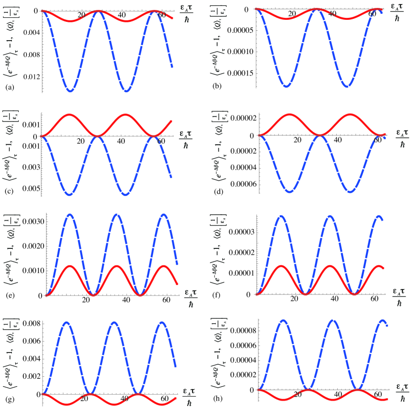
Figure 1: The quantities $\langle{\rm e}^{-\Delta\beta Q}\rangle_{\tau}-1$ (solid red line) and $\langle Q\rangle_{\tau}$ (broken blue line) in the two-spin 1/2 system. We fixed $\beta_{A}\epsilon_{A}=2$: for $\epsilon_{B}/\epsilon_{A}=0.8$, $\beta_{B}/\beta_{A}=0.9$ with (a) $\gamma J/\epsilon_{A}=0.1$ and (b) $\gamma J/\epsilon_{A}=0.01$; for $\epsilon_{B}/\epsilon_{A}=0.8$, $\beta_{B}/\beta_{A}=1.1$ with (c) $\gamma J/\epsilon_{A}=0.1$ and (d) $\gamma J/\epsilon_{A}=0.01$; for $\epsilon_{B}/\epsilon_{A}=1.25$, $\beta_{B}/\beta_{A}=0.9$ with (e) $\gamma J/\epsilon_{A}=0.1$ and (f) $\gamma J/\epsilon_{A}=0.01$; for $\epsilon_{B}/\epsilon_{A}=1.25$, $\beta_{B}/\beta_{A}=1.1$ with (g) $\gamma J/\epsilon_{A}=0.1$ and (h) $\gamma J/\epsilon_{A}=0.01$.

Note that $\langle{\rm e}^{-\Delta\beta Q}\rangle_{\tau}-1$ and $\langle Q\rangle_{\tau}$ have the same dependence on $\gamma$ in this model. Thus, the ratio of these two quantities is independent of the coupling strength $\gamma$:

$$\frac{\langle{\rm e}^{-\Delta\beta Q}\rangle_{\tau}-1}{\langle Q\rangle_{\tau}/(\frac{\epsilon_{A}}{2})} =\frac{\sinh\left[\frac{\epsilon_{A}}{2}(\beta_{B}-\beta_{A})\right]\sinh\left[\frac{\beta_{B}}{2}(\epsilon_{A}-\epsilon_{B})\right]}{\sinh\left[\frac{1}{2}(\beta_{B}\epsilon_{B}-\beta_{A}\epsilon_{A})\right]}.$$ (49)

Figure 2 shows the parameter dependence of the ratio. The ratio has a finite value for almost all range of the energy-level difference $\epsilon_{B}-\epsilon_{A}$.

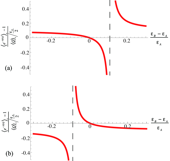
Figure 2: The ratio of the $\langle{\rm e}^{-\Delta\beta Q}\rangle_{\tau}-1$ to $\langle Q\rangle_{\tau}$. We fixed $\beta_{A}\epsilon_{A}=2$ with (a) $\beta_{B}/\beta_{A}=0.9$ and (b) $\beta_{B}/\beta_{A}=1.1$. The commutable-coupling condition is fulfilled at the point $\epsilon_{B}-\epsilon_{A}=0$.

As a consequence, if the coupling strength $\gamma$ is weak enough to neglect the deviation from the integral exchange fluctuation theorem, Eq. (47), the net heat transfer $\langle Q\rangle_{\tau}$ in Eq. (48) is also negligibly small. This result clearly shows that the exchange fluctuation theorem does not generally hold in the presence of a finite heat transfer.

However, the ratio in Fig. 2 vanishes for $\epsilon_{A}=\epsilon_{B}$; that is, the integral exchange fluctuation theorem is recovered at this particular point with a finite heat transfer. At this point $\epsilon_{A}=\epsilon_{B}$ and at this point only, the commutable-coupling condition is satisfied:

$$[H_{0},H_{\rm c}] =i\frac{J}{4}\left(\epsilon_{A}-\epsilon_{B}\right)\left(\sigma^{y}_{A}\sigma^{x}_{B}-\sigma^{x}_{A}\sigma^{y}_{B}\right)=0.$$ (50)

Under the commutable-coupling condition $\epsilon_{A}=\epsilon_{B}$, Eqs. (47) and (48) become

$$\langle{\rm e}^{-\Delta\beta Q}\rangle_{\tau}-1=0,$$ (51)

$$\langle Q\rangle_{\tau}=\frac{\epsilon}{2}\mathop{\mathrm{sech}}\left[\frac{\epsilon}{2}\beta_{A}\right]\mathop{\mathrm{sech}}\left[\frac{\epsilon}{2}\beta_{B}\right]\sinh\left[\frac{\epsilon}{2}\left(\beta_{B}-\beta_{A}\right)\right]\sin^{2}\left[\frac{\gamma J}{2\hbar}\tau\right].$$ (52)

The net heat transfer has a finite value, while the integral exchange fluctuation theorem holds. Thus we demonstrated in this model that the integral exchange fluctuation theorem holds if and only if the commutable-coupling condition is satisfied.

4.2 Coupled harmonic oscillators

The second example is a system which consists of two harmonic oscillators. This system is given by the following Hamiltonian:

$$H =H_{0}+\gamma H_{\rm c},$$ (53)

$$H_{0} =H_{A}\otimes 1_{B}+1_{A}\otimes H_{B}.$$ (54)

Here the Hamiltonian $H_{A}$, $H_{B}$ and $H_{\rm c}$ are

$$H_{A} =\hbar\omega_{A}a^{\dagger}a,$$

$$H_{B} =\hbar\omega_{B}b^{\dagger}b,$$

$$H_{\rm c} =\nu\left(a^{\dagger}b+b^{\dagger}a\right),$$ (55)

where $a$ and $a^{\dagger}$ are the creation and annihilation operators of the oscillator $A$, $b$ and $b^{\dagger}$ are those of $B$, $\left[a,a^{\dagger}\right]=1,\left[a,a\right]=0$ and $\left[b,b^{\dagger}\right]=1,\left[b,b\right]=0$, and $\nu$ is a real number.

To the second order of the coupling strength $\gamma$, the deviation from the integral exchange fluctuation theorem, $\langle{\rm e}^{-\Delta\beta Q}\rangle_{\tau}-1$, and the heat transfer $\langle Q\rangle_{\tau}$ are analytically calculated as follows:

$$\langle e^{-\Delta\beta Q}\rangle_{\tau}-1= 4\left\{\frac{\gamma\nu}{\hbar}\frac{\sin\left[\frac{\tau}{2}(\omega_{A}-\omega_{B})\right]}{(\omega_{A}-\omega_{B})/2}\right\}^{2}$$

$$\times\frac{\sinh\left(\Delta\beta\hbar\omega_{A}/2\right)\sinh\left[\beta_{B}\hbar(\omega_{A}-\omega_{B})/2\right]}{\left[2\sinh\left(\frac{\beta_{A}\hbar\omega_{A}}{2}\right)\right]\left[2\sinh\left(\frac{\beta_{B}\hbar\omega_{B}}{2}\right)\right]}+\mathrm{O}(\gamma^{3}),$$ (56)

$$\langle Q\rangle_{\tau}= -2\left\{\frac{\gamma\nu}{\hbar}\frac{\sin\left[\frac{\tau}{2}(\omega_{A}-\omega_{B})\right]}{(\omega_{A}-\omega_{B})/2}\right\}^{2}$$

$$\times\frac{\hbar\omega_{A}\sinh\left[(\beta_{A}\hbar\omega_{A}-\beta_{B}\hbar\omega_{B})/2\right]}{\left[2\sinh\left(\frac{\beta_{A}\hbar\omega_{A}}{2}\right)\right]\left[2\sinh\left(\frac{\beta_{B}\hbar\omega_{B}}{2}\right)\right]}+\mathrm{O}(\gamma^{3}).$$ (57)

The $\tau$ dependence of the deviation from the integral exchange fluctuation theorem and the net heat transfer during $\tau$ are shown in Fig. 3.

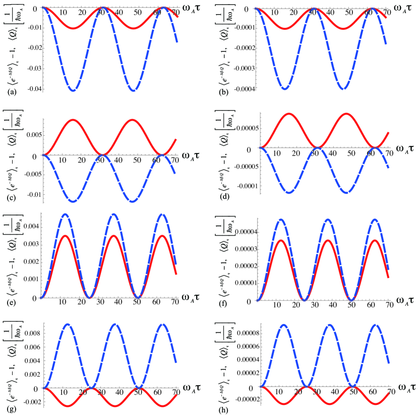
Figure 3: The quantities $\langle{\rm e}^{-\Delta\beta Q}\rangle_{\tau}-1$ (solid red line) and $\langle Q\rangle_{\tau}$ (broken blue line) in the coupled harmonic oscillators. We fixed $\beta_{A}\hbar\omega_{A}=4$: for $\omega_{B}/\omega_{A}=0.8$, $\beta_{B}/\beta_{A}=0.9$ with (a) $\gamma\nu/\hbar\omega_{A}=0.1$ and (b) $\gamma\nu/\hbar\omega_{A}=0.01$; for $\omega_{B}/\omega_{A}=0.8$, $\beta_{B}/\beta_{A}=1.1$ with (c) $\gamma\nu/\hbar\omega_{A}=0.1$ and (d) $\gamma\nu/\hbar\omega_{A}=0.01$; for $\omega_{B}/\omega_{A}=1.25$, $\beta_{B}/\beta_{A}=0.9$ with (e) $\gamma\nu/\hbar\omega_{A}=0.1$ and (f) $\gamma\nu/\hbar\omega_{A}=0.01$; for $\omega_{B}/\omega_{A}=1.25$, $\beta_{B}/\beta_{A}=1.1$ with (g) $\gamma\nu/\hbar\omega_{A}=0.1$ and (h) $\gamma\nu/\hbar\omega_{A}=0.01$.

To the second order of the coupling strength $\gamma$, the ratio of the above two quantities is given by

$$\frac{\langle{\rm e}^{-\Delta\beta Q}\rangle_{\tau}-1}{\langle Q\rangle_{\tau}/(\frac{\hbar\omega_{A}}{2})} =\frac{\sinh\left(\Delta\beta\hbar\omega_{A}/2\right)\sinh\left[\beta_{B}\hbar(\omega_{A}-\omega_{B})/2\right]}{\sinh\left[\hbar(\beta_{B}\omega_{B}-\beta_{A}\omega_{A})/2\right]}+\mathrm{O}(\gamma^{3}).$$ (58)

This result again shows that the exchange fluctuation theorem does not generally hold in the presence of a finite heat transfer.

However, we can see that the integral fluctuation theorem holds in the presence of a finite heat transfer at the point given by $\omega_{A}=\omega_{B}$. At this point and at this point only, the commutable-coupling condition is satisfied as

$$[H_{0},H_{\rm c}]=\hbar\nu(\omega_{A}-\omega_{B})(a^{\dagger}b-b^{\dagger}a)=0.$$ (59)

For the more general coupling Hamiltonian, $H_{\rm c}=\nu\left[(a^{\dagger})^{l_{A}}b^{l_{B}}+(b^{\dagger})^{l_{B}}a^{l_{A}}\right]$, the deviation from the integral exchange fluctuation theorem and the net heat transfer are calculated to the second order of $\gamma$ as

$$\langle e^{-\Delta\beta Q}\rangle_{\tau}-1= \left\{\frac{\gamma\nu}{\hbar}\frac{\sin\left[\frac{\tau}{2}(\omega_{A}l_{A}-\omega_{B}l_{B})\right]}{(\omega_{A}l_{A}-\omega_{B}l_{B})/2}\right\}^{2}$$

$$\times\frac{4l_{A}!\ l_{B}!}{\left[2\sinh\left(\beta_{A}\hbar\omega_{A}/2\right)\right]^{l_{A}}\left[2\sinh\left(\beta_{B}\hbar\omega_{B}/2\right)\right]^{l_{B}}}$$

$$\times\sinh\left(\Delta\beta\hbar\omega_{A}\l_{A}/2\right)\sinh\left[\beta_{B}\hbar(\omega_{A}l_{A}-\omega_{B}l_{B})/2\right]+\mathrm{O}(\gamma^{3}),$$ (60)

$$\langle Q\rangle_{\tau}= \left\{\frac{\gamma\nu}{\hbar}\frac{\sin\left[\frac{\tau}{2}(\omega_{A}l_{A}-\omega_{B}l_{B})\right]}{(\omega_{A}l_{A}-\omega_{B}l_{B})/2}\right\}^{2}$$

$$\times\frac{-2l_{A}!\ l_{B}!}{\left[2\sinh\left(\beta_{A}\hbar\omega_{A}/2\right)\right]^{l_{A}}\left[2\sinh\left(\beta_{B}\hbar\omega_{B}/2\right)\right]^{l_{B}}}$$

$$\times\hbar\omega_{A}l_{A}\sinh\left[(l_{A}\beta_{A}\hbar\omega_{A}-l_{B}\beta_{B}\hbar\omega_{B})/2\right]+\mathrm{O}(\gamma^{3}).$$ (61)

The ratio of the above two quantities is given by

$$\frac{\langle{\rm e}^{-\Delta\beta Q}\rangle_{\tau}-1}{\langle Q\rangle_{\tau}/(\frac{\hbar\omega_{A}l_{A}}{2})} =\frac{\sinh\left(\Delta\beta\hbar\omega_{A}l_{A}/2\right)\sinh\left[\beta_{B}\hbar(\omega_{A}l_{A}-\omega_{B}l_{B})/2\right]}{\sinh\left[\hbar(\beta_{B}\omega_{B}l_{B}-\beta_{A}l_{A}\omega_{A})/2\right]}+\mathrm{O}(\gamma^{3}).$$ (62)

This shows that the integral exchange fluctuation theorem holds in the presence of a finite heat transfer if and only if the commutable-coupling condition is satisfied:

$$[H_{0},H_{\rm c}]=\hbar\nu(\omega_{A}l_{A}-\omega_{B}l_{B})\left[(a^{\dagger})^{l_{A}}b^{l_{B}}-(b^{\dagger})^{l_{B}}a^{l_{A}}\right]=0,$$ (63)

or $\omega_{A}l_{A}=\omega_{B}l_{B}$.

5 Conclusions

To summarize, we showed that the exchange fluctuation theorem in its original form does not generally hold in the presence of a finite heat transfer. In the limit $\gamma\to 0$, the $k$th moments of $p_{\tau}(Q)$ vanish for $k\geq 1$. The deviation from the exchange fluctuation theorem also vanishes in the same order of $\gamma$. We derived general formulas for the above and analytically confirmed them for specific models. This means that there is no heat transfer when the coupling strength $\gamma$ is small enough to neglect the deviation from the exchange fluctuation theorem. In this case, the exchange fluctuation theorem reduces to a trivial relation and has no information about the heat transfer.

However, we found a condition for the exchange fluctuation theorem to hold exactly for arbitrary $\gamma$ and we referred to it as the commutable-coupling condition. Under this condition, the exchange fluctuation theorem becomes an exact relation independently of the coupling strength $\gamma$ under the existence of a finite heat transfer. We confirmed this in specific models. In short, the exchange fluctuation theorem holds not because the coupling is weak as was originally proposed, but because the total energy of the system is conserved under the commutable-coupling condition.

The deviation from the exchange fluctuation theorem consists of the commutation relation between the Hamiltonian of the total system and the coupling Hamiltonian. Therefore, the non-commutativity of the observable in quantum mechanics plays an important role in the deviation.

References

- [1] D. J. Evans, E. G. D. Cohen, and G. P. Morriss, Phys. Rev. Lett. 71 (1993), 2401.
- [2] D. J. Evans, D. J. Searles, Phys. Rev. E. 50 (1994), 1645.
- [3] G. Gallavotti and E. G. D. Cohen, Phys. Rev. E. 74 (1995), 2694.
- [4] J. Kurchan, J. Phys. A: Math. Gen. 31 (1998), 3719.
- [5] J. L. Lebowitz and H. Spohn, J. Stat. Phys. 95 (1999), 333.
- [6] C. Jarzynski, Phys. Rev. Lett. 78 (1997), 2690.
- [7] G. E. Crooks, J. Stat. Phys. 90 (1998), 1481.
- [8] G. E. Crooks, Phys. Rev. E. 60 (1999), 2721.
- [9] D. J. Evans and D. J. Searses, Adv. Phys. 51 (2002), 1529.
- [10] E. M. Sevick, R. Prabhakar, S. R. Williams, and D. J. Searles, Annu. Rev. Phys. Chem. 59 (2008), 603.
- [11] D. M. Carberry, J. C. Reid, G. M. Wang, E. M. Sevick, D. J. Searles, and D. J. Evans, Phys. Rev. Lett. 92 (2004), 140601.
- [12] J. Liphardt, S. Dumont, S. B. Smith, I. Tinoco (Jr), and C. Bustamante, Science 296 (2002), 1832.
- [13] D. Collin, F. Ritort, C. Jarzynski, S. B. Smith, I. Tinoco (Jr), and C. Bustamante, Nature 437 (2005), 231.
- [14] S. Yukawa, J. Phys. Soc. Jpn. 69 (2000), 2367.
- [15] T. Monnai and S. Tasaki, cond-mat/0308337.
- [16] A. E. Allahverdyan and Th. M. Nieuwenhuizen, Phys. Rev. E 71 (2005), 066102.
- [17] M. F. Gelin and D. S. Kosov, Phys. Rev. E 78 (2008), 01116.
- [18] J. Kurchan, cond-mat/0007360.
- [19] H. Tasaki, cond-mat/0009244.
- [20] S. Mukamel, Phys. Rev. Lett. 90 (2003), 170604.
- [21] T. Monnai, Phys. Rev. E. 72 (2005), 027102.
- [22] P. Talkner, E. Lutz, and P. Hanggi, Phys. Rev. E. (R)75 (2007), 050102.
- [23] C. Jarzynski and D. K. Wójcik, Phys. Rev. Lett. 92 (2004), 230602.
- [24] J. J. Sakurai, Modern Quantum Mechanics, (Benjamin, Menlo Park, California, 1985).
- [25] J. Teifel and G. Mahler, Phys. Rev. E 76 (2007), 051126.