Vortex-vortex interaction in thin superconducting films

Abstract

The properties of vortices in superconducting thin films are revisited. The interaction between two Pearl vortices in an infinite film is approximated at all distances by a simple expression. The interaction of a vortex with a regular lattice of real or image vortices is given. The two spring constants are calculated that one vortex in the vortex lattice feels when the surrounding vortices are rigidly pinned or are free. The modification of these London results by the finite size of real films is obtained. In finite films, the interaction force between two vortices is not a central force but depends on both vortex positions, not only on their distance. At the film edges the interaction energy is zero and the interaction force is peaked. Even far from the edges the vortex interaction considerably deviates from the Pearl result and is always smaller than it.

I Introduction

In this note the problem of vortices in thin superconducting films is revisited. Useful formulae for the interaction between vortices in thin superconducting films within London Theory are given when the film thickness $d$ is smaller than the London penetration depth $\lambda$. In such thin films the vortex interaction is mediated mainly by the magnetic stray field, and the screening of the in-plane supercurrents is governed by the effective 2-dimensional (2D) penetration depth $\Lambda=\lambda^{2}/d>\lambda>d$. The current density $j(x,y,z)$ in thin films is nearly independent of the $z$ coordinate (perpendicular to the film) and the sheet current in the film is thus ${\bf J}(x,y)=\int_{-d/2}^{d/2}{\bf j}(x,y,z)dz\approx{\bf j}d$. The sheet current of a vortex in such a thin film and the interaction force between two vortices was calculated first by Judea Pearl 1 for an infinitely large film. For infinite films of arbitrary thickness the Pearl-London vortex and the vortex-vortex interaction were calculated analytically, 2 ; 3 ; 4 and the Ginzburg-Landau (GL) theory for periodic vortex lattices in such films with arbitrary GL parameter $\kappa$ in the entire range of inductions $\bar{B}$ was computed in Ref. 5, .

For superconductors of finite size, recently there have been numerous computations based on the static or time-dependent GL equations for small (mesoscopic) specimens containing a few vortices, also giant vortices with several flux quanta, and considering the equilibrium state or the penetration, exit, nucleation, and annihilation of vortices. For example, superconducting disks are considered in Ref. 5a126, ; 5a118, ; 5a115117, ; 5a78, ; 5a61, ; 5a34, ; 5aZhou, , squares and other shapes in Ref. 5b105, ; 5b84, ; 5b66, ; 5b45, , also squares containing magnetic dots 5c13 ; 5c6988 or antidots or blind holes 5d84 ; 5d66 as pinning centers, and disks in inhomogeneous magnetic field.5e99 When the 2D penetration depth $\Lambda=\lambda^{2}/d$ is much larger than the film size, the energy of the magnetic stray field outside the specimen is expected to be negligible and analytical approximations can be made.5f71 Further work computes the properties of infinitely long straight vortices in semi-infinite 5gHern or cylindrical 5hSard samples and argues that these results apply also to thin films in a perpendicular field in cases when the magnetic stray-field energy outside the film may be disregarded.

The present paper focusses on situations when the stray-field energy is not negligible, e.g., since $\Lambda$ is smaller than the film size, and it is restricted to the London limit in which the superconducting coherence length $\xi$ and vortex core radius $r_{c}\approx\xi$ are much smaller than the film size and than $\Lambda$. In Sec. II we first consider the limit of ideal screening ($\Lambda=0$) when the sheet current and energy of vortices are completely determined by the stray field and can be derived easily for an infinite film. Introduction of a finite $\Lambda$ then leads to Pearl vortices, whose interaction is discussed in some detail in Sec. II-V and in Appendix A. Finally, in Sec. VI vortices and their interaction in films of finite size are presented, computed by a method 6 ; 7 that applies to thin flat films of any size and shape and to any $\Lambda$. As a main result in Sec. VII it will be shown that the sheet current and interaction of vortices in films of finite size differ considerably from the ideal Pearl result. As expected, this deviation is most pronounced near the film edges, where the real interaction potential vanishes while the interaction force is peaked. But less expectedly, this deviation is considerable even when the interacting vortex pair is located far from the film edges, e.g., near the center of a square film: The real interaction with a central vortex is reduced from its Pearl value by a factor which decreases approximately linearly from unity to zero as one goes from the central vortex towards the edge, see Fig. 6 below. A summary is given in Sec. VIII.

II Vortices in thin infinite films

The thin-film problem differs from the behavior of currents and vortices in bulk superconductors by the dominating role of the magnetic stray field outside the film. The interaction between vortices occurs mainly by this stray field and thus has very long range (interacting over the entire film width), while in bulk superconductors the vortex currents and the vortex interaction are screened and thus decrease exponentially over the length $\lambda$.

The long-range currents and forces can be shown for the ideal screening limit of zero $\lambda$ as follows. Consider one vortex in the center of a large circular film with radius $R\to\infty$. On length scales larger than $\lambda$ this point vortex behaves like a magnetic dipole, composed of two magnetic monopoles: one sends magnetic flux $\Phi_{0}$ into the space above the film and one receives the same flux from the lower half space. Here $\Phi_{0}=h/2e=2.07\cdot 10^{-15}$ Tm² is the quantum of magnetic flux. The magnetic field lines of this point-vortex are straight radial lines, all passing through this point. The magnitude of this magnetic stray field is $\Phi_{0}/(2\pi r_{3}^{2})$ above and $-\Phi_{0}/(2\pi r_{3}^{2})$ below the film, since the flux $\Phi_{0}$ has to pass through the shell of any half sphere of 3D radius $r_{3}=(r^{2}+z^{2})^{1/2}$ and surface area $2\pi r_{3}^{2}$. Here $r=(x^{2}+y^{2})^{1/2}$ is the 2D radius in the film plane $z=0$. Directly above and below the film plane the stray field has the same magnitude $\Phi_{0}/(2\pi r^{2})$ but has opposite sign. This jump of the magnetic field component parallel to the film is caused by a sheet current that circulates around the vortex and equals this field difference in size, $J(r)=\Phi_{0}/(\mu_{0}\pi r^{2})$. This current thus decreases very slowly with radius $r$. The force $F$ between this central vortex and a second vortex at a distance $r$ is radial (central force) and repulsive and in size equals just this sheet current $J(r)$ times the flux quantum $\Phi_{0}$,

$$F(r)=\Phi_{0}J(r)={\Phi_{0}^{2}\over\mu_{0}\,\pi\,r^{2}}.$$ (1)

The interaction potential $V(r)$ between these two point vortices (Pearl vortices) follows from its derivative $F(r)=-V(r)^{\prime}$ and the definition $V(\infty)=0$,

$$V(r)={\Phi_{0}^{2}\over\mu_{0}\,\pi\,r}.$$ (2)

Note that this result does not depend on $\Lambda=\lambda^{2}/d$. It applies also for finite $\Lambda$ if the distance is large, $r\gg\Lambda$.

The general results for arbitrary $\Lambda$ can be derived from the expression for the interaction potential noting that still $F(r)=-V(r)^{\prime}$ and $J(r)=F(r)/\Phi_{0}$. One has

$$V(r)={\Phi_{0}^{2}\over\mu_{0}}\int\!{d^{2}k\over 4\pi^{2}}{2\cos{\bf kr}\over k+2\Lambda k^{2}}={\Phi_{0}^{2}\over\mu_{0}}\int_{0}^{\infty}\!\!{dk\over 2\pi}{2J_{0}(kr)\over 1+2\Lambda k}\,,$$ (3)

where $J_{0}(x)$ is a Bessel function and $k^{2}=k_{x}^{2}+k_{y}^{2}$. The limits for small and large distances are, 1 see also  Eq. (2),

$$V(r) \approx {\Phi_{0}^{2}\over\mu_{0}}~{}{\ln(2.27\Lambda/r)\over 2\pi\Lambda}~{}\,~{}{\rm for~{}~{}}r\ll\Lambda\,,$$ (4)

$$V(r) \approx {\Phi_{0}^{2}\over\mu_{0}}~{}{1\over\pi r}~{}~{}~{}~{}~{}~{}~{}~{}~{}~{}~{}~{}~{}~{}~{}{\rm for~{}~{}}r\gg\Lambda\,.$$ (5)

The factor 2.27 is a fitted constant that follows from the numerical evaluation of the integral (3). An excellent fit to the exact result valid for all distances $0<r<\infty$ and all $\Lambda$ is within line thickness

$$V(r)\approx{\Phi_{0}^{2}\over 2\pi\Lambda\mu_{0}}~{}\ln\Bigg{(}\,{2.27\Lambda\over r}-{0.27\Lambda\over 9\Lambda+r}+1\Bigg{)}.$$ (6)

Figure 1 shows the exact potential from Eq. (3), its limits (4) and (5), and the approximation (6). One can see that the expression (6) (dots) practically coincides with the exact potential (solid line).

In the original paper by Pearl 1 the force $f_{12}(r)=-V^{\prime}(r)$ between two point vortices was expressed in terms of Struve and Neumann functions $S_{1}$ (or ${\bf H}_{n}$) and $N_{1}$ (or $Y_{n}$, the Bessel function of the second kind, or Weber function),8

$$f_{12}(r)={\Phi_{0}^{2}\over 8\Lambda^{2}\mu_{0}}~{}\Big{[}\,{\bf H}_{1}\Big{(}{r\over 2\Lambda}\Big{)}-Y_{1}\Big{(}{r\over 2\Lambda}\Big{)}-{2\over\pi}\Big{]}\,.$$ (7)

Though both $S_{1}$ and $N_{1}$ are oscillating functions this force $f_{12}$ is monotonic and agrees with $-V^{\prime}(r)$, Eq. (3). The interaction potential $V(r)$ may be also expressed in terms of Struve and Weber functions, see appendix in 9 ,

$$V(r)={\Phi_{0}^{2}\over 4\Lambda\mu_{0}}~{}\Big{[}\,{\bf H}_{0}\Big{(}{r\over 2\Lambda}\Big{)}-Y_{0}\Big{(}{r\over 2\Lambda}\Big{)}\Big{]}\,.$$ (8)

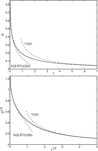
Figure 1: The interaction potential $V(r)$, Eq. (3), between two Pearl vortices (solid lines), the limits (4) and (5) (dashed lines) and the approximation (6) (dots). $V$ is in units $\Phi_{0}^{2}/(\mu_{0}\Lambda)$ and $r$ in units $\Lambda=\lambda^{2}/d$. The upper plot shows directly $V(r)$. The lower plot shows $\sqrt{V}$ versus $\sqrt{r}$ to depict larger ranges of $V$ and $r$ and to show the validity of the limiting expressions at small and large $r$ more clearly.

III Interaction with vortex lattices

Next I consider the interaction potential $V({\bf r})$ between a vortex at position ${\bf r}=(x,y)$ in the film and a regular lattice of vortices sitting at ideal-lattice points ${\bf R}$ with reciprocal lattice vectors ${\bf K}$. This situation can be interpreted in two ways:

1. This lattice can consist of real vortices in the film, generated by a constant applied magnetic field $B_{a}$ perpendicular to the film plane (along $z$). In this case it will be typically a triangular lattice with density $n=B_{a}/\Phi_{0}$, since the magnetic field has to penetrate the infinitely extended film completely, i.e., the average induction $\bar{B}$ equals $B_{a}$. The lattice spacing is then $a\approx(\Phi_{0}/\bar{B})^{1/2}$.

2. In a second application the lattice may be formed by the image vortices sitting on a superlattice that is constructed to achieve periodic boundary conditions in the numerical simulation of a film with vortex pinning. In this case the superlattice may be chosen such that the basic cell is a rectangle with side lengths ($L_{x},L_{y}$). The regular lattice positions are then ${\bf R}=(\mu L_{x},\nu L_{y})$ where $\mu,\nu=0,\pm 1,\pm 2,\dots$ are integers, and the reciprocal lattice vectors are ${\bf K}=(2\pi\mu/L_{x},2\pi\nu/L_{y})$.

The interaction potential between the probing vortex at position ${\bf r}$ and the periodic lattice of vortices (or images) is obtained by linear superposition of potentials of the form (3),

$$V_{\rm per}({\bf r})={\Phi_{0}^{2}\over\mu_{0}}\int\!{d^{2}k\over 4\pi^{2}}\sum_{\bf R}{2\exp[i{\bf k(r-R)}]\over k+2\Lambda k^{2}}\,.$$ (9)

This potential is periodic, $V_{\rm per}({\bf r+R})=V_{\rm per}({\bf r})$. The infinite lattice sum in (8) can be evaluated using the formula

$$\sum_{\bf R}\exp(i{\bf kR})=4\pi^{2}n\sum_{\bf K}\delta_{2}({\bf k-K})\,,$$ (10)

where $n$ is the density of lattice points ${\bf R}$; the density of reciprocal lattice points is $1/(4\pi^{2}n)$. Inserting (10) into (9) and performing the ${\bf k}$ integration over the 2D delta functions $\delta_{2}({\bf k-K})$ one obtains

$$V_{\rm per}({\bf r})={\Phi_{0}^{2}\,n\over\mu_{0}}\sum_{{\bf K}\neq 0}{2\cos({\bf Kr})\over K+2\Lambda K^{2}}\,.$$ (11)

This periodic potential may be used for computer simulation of vortex pinning in a thin film with periodic boundary conditions. In this case the super-lattice density is $n=1/(L_{x}L_{y})$.

Next I apply this potential to the following problem. Consider a regular (e.g. triangular) vortex lattice in the film in which all vortices are pinned to these ideal vortex positions and the central vortex at ${\bf R}=0$ is moved a bit in $x$ direction. Which interaction potential with all other vortices does this central vortex see? To obtain this potential $V_{c}({\bf r})$, or its curvature $V_{c}^{\prime\prime}(0)=\partial^{2}V_{c}({\bf r})/\partial x^{2}$ at ${\bf r}=0$, we have to subtract from the complete lattice sum (9) the term with ${\bf R}=0$, since this term describes the interaction of the shifted vortex at ${\bf r}\approx 0$ with the unshifted vortex at ${\bf R}=0$, which would be very large and diverging as ${\bf r\to R}$. The resulting potential is

$$V_{c}({\bf r})={\Phi_{0}^{2}\over\mu_{0}}\int\!{d^{2}k\over 4\pi^{2}}\sum_{{\bf R}\neq 0}{2\exp[i{\bf k(r-R)}]\over k+2\Lambda k^{2}}~{}~{}~{}~{}$$

$$={\Phi_{0}\bar{B}\over\mu_{0}}\Big{[}\sum_{{\bf K}\neq 0}{2\cos({\bf Kr})\over K+2\Lambda K^{2}}-\!\int\!{d^{2}k\over 4\pi^{2}n}\,{2\cos({\bf kr})\over k+2\Lambda k^{2}}\Big{]}\,.$$ (12)

with $\bar{B}=n\Phi_{0}$. This result is still general and applies to any ${\bf r}$. To obtain its curvature at ${\bf r}=0$ we apply to it the Laplace operator $\nabla^{2}=\partial^{2}/\partial x^{2}+\partial^{2}/\partial y^{2}$. This creates a factor $-K^{2}$ in the sum and a factor $-k^{2}$ in the integral. Due to symmetry of the triangular (and also the square) vortex lattice, the curvature of $V_{c}({\bf r})$ at ${\bf r}=0$ is the same along all directions, i.e., one has $V_{c}({\bf r})=V_{c}(0)+{1\over 2}V_{c}^{\prime\prime}(0)r^{2}+O(x^{4},x^{2}y^{2},y^{4})$ with $V_{c}^{\prime\prime}(0)=\partial^{2}V_{c}/\partial x^{2}=\partial^{2}V_{c}/\partial y^{2}={1\over 2}\nabla^{2}V_{c}$ at $x=y=0$. The result for this curvature is thus

$$V_{c}^{\prime\prime}(0)={\Phi_{0}\bar{B}\over 2\mu_{0}}\Big{[}\!\int\!\!{d^{2}k\over 4\pi^{2}n}\,{2k^{2}\over k\!+2\Lambda k^{2}}-\!\sum_{{\bf K}\neq 0}{2K^{2}\over K\!\!+\!2\Lambda K^{2}}\Big{]}.\,$$ (13)

The sum and the integral in (13) largely compensate. This may be seen by formally introducing an upper boundary $k_{\rm max}=K_{\rm max}$, which makes the integral and the sum finite but drops out from their difference. The main contribution to this difference comes from the integral at small $k\leq k_{B}$, where $k_{B}$ is the radius of the Brillouin zone approximated by a circle. One has $k_{B}^{2}=4\pi n$ for all vortex lattice symmetries.

For $\Lambda$ larger than the vortex spacing $a$, one has $\Lambda K\gg 1$ for all $K$. More precisely, the condition is $K_{10}^{2}=16\pi^{2}/(3a^{2})\gg\Lambda^{-2}$, thus $2\pi\Lambda\gg a$ is sufficient. In this case the general result (13) may be evaluated approximately by keeping just the integral over $0<k\leq k_{B}$ and noting that the remaining integral for $k>k_{B}$ is compensated by the sum over ${\bf K}\neq 0$. The final result for the curvature in this limit is then

$$V_{c,\infty}^{\prime\prime}(0)={\Phi_{0}\bar{B}\over 2\mu_{0}\Lambda}={\Phi_{0}\bar{B}d\over 2\mu_{0}\lambda^{2}}\,.$$ (14)

IV Results from Elasticity

The spring constant (14) may be calculated also from the elasticity theory of the vortex lattice, 10 ; 11 ; 12 see Appendix A. In this case one requires nonlocal elasticity with a dispersive compressional modulus $c_{11}(k)$. The result coincides with Eq. (14).

In Appendix A also is calculated the spring constant $V^{\prime\prime}_{\rm elast}(0)$ felt by the central vortex when the surrounding vortices are not pinned but are held in place only by the interaction with their neighbors. In this case, the elastic response of the central vortex depends only on the shear modulus $c_{66}$ of the triangular vortex lattice, 10 ; 12 which is not dispersive. Thus, local elasticity theory is sufficient for this problem. However, now an inner cut-off radius $k_{\rm min}=1/R_{d}$ is required for the ${\bf k}$ integral, which is taken from the finite radius $R_{d}$ of the thin disk containing the vortex lattice. It is assumed that the vortices are pinned at the edge of the disk, at $r=R_{d}$. The resulting elastic spring constant is then

$$V^{\prime\prime}_{\rm elast}(0)={\bar{B}\,\Phi_{0}\over 4\mu_{0}\Lambda\ln(R_{d}k_{B})}={V^{\prime\prime}_{c,\infty}(0)\over 2\ln(\pi R_{d}/a)}\,.$$ (15)

This $V^{\prime\prime}_{\rm elast}(0)$ is smaller than the spring constant $V^{\prime\prime}_{c,\infty}(0)$ of the rigidly pinned vortex lattice by a factor $0.5/\ln(\pi R_{d}/a)$. A constant force $f_{0}$ on the central vortex thus displaces this vortex a distance $u_{0}$ that increases by a factor $2\ln(\pi R_{d}/a)$ when pinning of the surrounding vortices is switched off.

In all the above expressions the vortex core radius $r_{c}\approx\xi$ and the coherence length $\xi$ were assumed to be smaller than any other relevant length, in particular $\xi\ll\Lambda=\lambda^{2}/d$. This is the London limit. Finite $\xi$ is easily considered by taking the $k$ integral not to infinite $k$ but to some upper cut-off value $k_{\rm max}\approx 1/\xi$. This cut-off removes the logarithmic divergence of $V(r)\propto\ln(2.27\Lambda/r)$, Eq. (4), and smoothes it over the core radius $r_{c}\approx\xi$. This smoothing may also be performed by replacing in the logarithm $r$ by $(r^{2}+r_{c}^{2})^{1/2}$ as shown in Ref. 13, ; 14, ; 15, . The exact numerical solution of the GL equations for a vortex and the periodic vortex lattice in films of finite thickness is given in Ref. 5, . The London solution for a vortex in films of finite thickness is presented e.g. in Ref. 4, .

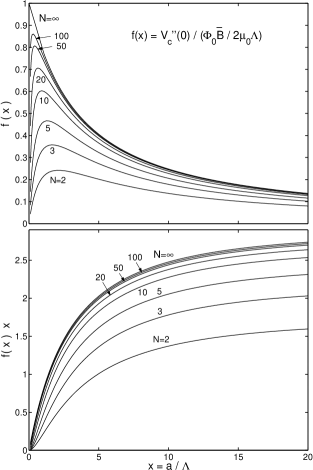
Figure 2: The reduced curvature $f(x,N)=V^{\prime\prime}_{c}(0,N)\cdot(2\mu_{0}\Lambda/\Phi_{0}\bar{B})$, Eq. (17), of the potential exerted on a central Pearl vortex by the surrounding $\pi N^{2}a^{2}$ pinned vortices within a circular area of radius $Na$. The function $f$ is plotted versus the reduced vortex spacing $x=a/\Lambda$ for several values of $N=2$ to $N=\infty$. While $f(x,N)$ (upper plot) for finite $N$ has a maximum and vanishes at small and large $x$, the product $f(x,N)\cdot x$ for all $N$ is monotonically increasing with $x$.

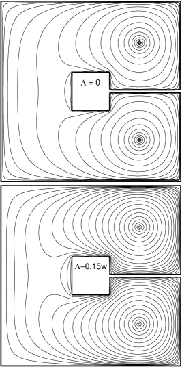
Figure 3: Current stream lines of a pair of vortices, coinciding with the contour lines of the vortex-vortex interaction. Shown are the contours of the logarithm of the interaction potential, Eq. (18), for a square thin superconducting film of size $2w\times 2w$ with slit and central square hole, containing a pair of Pearl vortices (due to the mirror symmetry of this computation) at $x_{i}=0.54w$, $y_{i}=\pm x_{i}$; $88\times 88$ grid points are used and 20 contours. The force exerted by this vortex pair on a third probing vortex at position $x,y$ acts perpendicular to these contour lines. Top: 2D penetration depth $\Lambda=0$ (ideal screening). Bottom: $\Lambda=0.15w$.

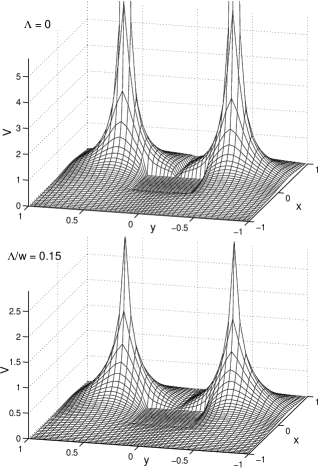
Figure 4: 3D plot of the interaction of a probing Pearl vortex positioned at $(x,y)$ with a pair of vortices sitting at $x_{i}=0.4w$, $y_{i}=\pm 0.5w$ in a thin square film of size $2w\times 2w$ with slit and hole. Plotted is the interaction potential, Eq. (18), in units $\Phi_{0}^{2}/(\mu_{0}w)$, versus $x,y$ in units of $w$; $46\times 46$ grid points are used. Top: $\Lambda=0$ (ideal screening). Bottom: $\Lambda=0.15w$.

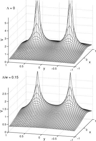
Figure 5: Same geometry as Fig. 4, but Pearl potential, Eq. (19). This approximate interaction potential between a probing Pearl vortex at $(x,y)$ with a pair of vortices at $x_{i}=0.4w$, $y_{i}=\pm 0.5w$ does not vanish at the edges of the square film and of its slit and hole, while the correct numerical interaction (18) depicted in Fig. 4 does vanish there.

V Vortex lattice of finite size

Expressions (12) to (14) apply to an infinitely extended vortex lattice. The finite size of the superconducting film can be approximately accounted for by taking the sums $\sum_{{\bf R}\neq 0}$ in Eq. (12) over a finite area only, e.g., over a circular area of radius $R_{d}=Na$ (disk radius), $|{\bf R}|<R_{d}$, containing $\approx\pi N^{2}$ vortices. The approximate potential that a central vortex sees in the presence of a regular lattice of pinned vortices in such a thin disk is thus

$$V_{c}({\bf r},N)=\sum_{\bf R}V({\bf r-R}),~{}~{}0<|{\bf R}|<Na\,.$$ (16)

For $N\to\infty$, Eq. (16) coincides with Eq. (12), and the curvatures coincide, $V_{c}^{\prime\prime}(0,\infty)=V_{c}^{\prime\prime}(0)$, Eq. (13). For finite $N$, the interaction and its curvature are reduced. To visualize this we define the dimensionless curvature

$$f(a/\Lambda,N)=V_{c}^{\prime\prime}(0,N)/V^{\prime\prime}_{c,\infty}(0)\,,$$ (17)

with $f(0,\infty)=1$. This function is shown in Fig. 2. One can see that the dense-lattice limit, Eq. (14), is a good approximation when $a\leq 2\Lambda$ and $N\geq 20$. For larger $a$ and smaller $N$ the reduced curvature $f(a/\Lambda,N)$ decreases. At small values of $x=a/\Lambda\leq 2$ for $N\geq 2$, $f(x)$ has a maximum and decreases to zero when $x\to 0$ because then also the disk radius $R_{d}=aN$ goes to zero.

VI Vortex interaction in films of finite size

The interaction potential and force between two vortices in thin films of finite size and arbitrary shape depends on the size and shape of the film. Moreover, it depends on the positions of both vortices, $V=V({\bf r}_{1},{\bf r}_{2})$, while for infinite films (Sec. I) $V(r)$ depends only on the distance $r=|{\bf r}_{1}-{\bf r}_{2}|$. These dependences are obvious from the fact that the interaction potential between two vortices has to vanish when one vortex approaches the edge of the film, where its magnetic flux goes to zero since supercurrents cannot circulate around a vortex core positioned on the edge. Furthermore, the interaction force in general is not a central force but close to the film edge the force on the second vortex is directed perpendicular to the edge no matter where the first vortex is positioned. This is so since the current generated by a vortex flows along the film edge close to the edge, see Fig. 3. Though the vortex interaction energy vanishes at the edges, the interaction force has a peak there which increases with decreasing $\Lambda$. Only when the two vortices are far from all film edges and are close to each other, then the central Pearl interaction potential $V(r)$ of Sec. I is a good approximation, see Sec. VII.

The vortex interaction in realistic films of finite extension can be computed by the method described in Ref. 6, ; 7, . One has $V({\bf r}_{i},{\bf r}_{j})=V_{ij}=V_{ji}=-\Phi_{0}g_{i}({\bf r}_{j})$ where $g_{i}({\bf r})$ is the stream function of the 2D sheet current density ${\bf J}_{i}({\bf r})$ caused by a vortex centered at ${\bf r}_{i}$. In general one has ${\bf J(r)}=-{\bf\hat{z}}\times\nabla g({\bf r})=\nabla\times({\bf\hat{z}}g)=(\partial g/\partial y,\,-\partial g/\partial x)$. The function $g({\bf r})=g(x,y)$ has several useful properties listed in Sec. 2A of Ref. 7, . In particular, its contour lines are the stream lines of the sheet current, and it may be put $g=0$ on the outer edge of the film, which coincides with a stream line if there is no current fed in by contacts.

The function $g(x,y)$ and its sheet current ${\bf J}(x,y)$ can be caused by an applied magnetic field, or by the flux trapped in a hole in the film, or by vortices, and also by applied currents, which we do not consider here. Within London theory all these contributions superimpose linearly. In Ref. 7, it is shown how these sheet currents can be computed by introducing a grid of $M$ equidistant or nonequidistant points ${\bf r}_{i}$ and then inverting a $M\times M$ matrix. The inverted matrix $K_{ij}^{\Lambda}$, Eq. (11) of Ref. 7, , (dimension m) is closely related to the vortex interaction. One has

$$V({\bf r}_{i},{\bf r}_{j})=V({\bf r}_{j},{\bf r}_{i})=-\mu_{0}^{-1}\,\Phi_{0}^{2}\,K_{ij}^{\Lambda}/w_{j}\,,$$ (18)

where $w_{i}$ are the weights of the grid points (dimension m²). This potential is repulsive (positive) and sharply peaked at ${\bf r}_{i}={\bf r}_{j}$, and like the function $g(x,y)$ it vanishes at the outer edge of the film. This vanishing is linear for $\Lambda>0$, while for $\Lambda=0$ (ideal screening) $g$ and $V$ go to zero like $\sqrt{\delta}$ where $\delta$ is the distance to the edge.

If the film contains one or more holes (is multiply connected) the $g(x,y)$ can have a non-zero value inside the hole, $g(x,y)=I=$ const, where $I$ is the total current that circles around the hole when the hole contains trapped magnetic flux. If the hole is connected with the outer edge by a slit, then its border is part of the outer edge and one has $g=0$ along the entire (inner and outer) edge of the film. If the slit is short-cut, one can trap flux in the slit and hole. If the slit is bridged by a superconducting weak link, this film can be used as a Superconducting Quantum Interference Device (SQUID). 7 ; 16

Figure 3 shows the contour lines of this vortex interaction, coinciding with the stream lines of the sheet current ${\bf J}(x,y)$ since $V\propto g$. Depicted are the contours of the logarithm of the interaction potential, Eq. (18), between a probing vortex sitting at $(x,y)$ and a pair of vortices at ($x_{i},\pm y_{i}$) since our computation assumes mirror symmetry about the $x$ axis, $\ln[V(x_{i},y_{i};\,x,y)+V(x_{i},-y_{i};\,x,y)]$. In the regions where $V$ is very small, this logarithm shows more contours than a linear contour plot would show.

Figure 4 shows the same interaction depicted as a 3D plot. Both Fig. 3 and Fig. 4 show the geometry of a thin superconducting square of size $2w\times 2w$ with a central square hole and an open slit, which may be used as a SQUID. Depicted are the cases $\Lambda=0$ (ideal screening) and $\Lambda/w=0.15$. One can see that for $\Lambda=0$ the potential $V$ and the stream function $g$ at the edges go to zero with vertical slope, $V\propto g\propto\sqrt{\delta}$ ($\delta=$ distance to the edge), and for finite $\Lambda$, $V\propto g\propto\delta$ vanish linearly at the inner and outer edges of the film. In Fig. 4, a grid of only $46\times 46$ nonequidistant points is chosen such that no grid points sit directly on the film edges. Therefore, on the grid points closest to the outer edges of the film the depicted $V$ is not exactly zero even when it is zero on the very edges.

Figure 5 shows, for the same geometry and grid as in Fig. 4, the approximate vortex-vortex interaction obtained from the Pearl potential of Sec. 1 valid for an infinite film. To allow comparison with the correct numerical potential of Fig. 4, which has mirror symmetry, we symmetricize this approximate potential by plotting

$$V({\bf r},{\bf r}_{i}) = V\big{[}\big{(}(x-x_{i})^{2}+(y-y_{i})^{2}+\epsilon\big{)}^{1/2}\big{]}$$ (19)

$$+ V\big{[}\big{(}(x-x_{i})^{2}+(y+y_{i})^{2}+\epsilon\big{)}^{1/2}\big{]}\,,$$

where $V(r)$ is the Pearl interaction of Sec. I, e.g., Eq. (6). The cut-off $\epsilon=4\cdot 10^{-4}w^{2}$ was chosen to reach the same peak heights as in Fig. 4. Note that the numerical interaction potential, Eq. (18) and Fig. 4, has a natural cut-off and finite peak heights, which are related to the spacing of the grid points. The peaks of the numerical $V$ (Fig. 4) are well approximated by the cut-off Pearl peaks of Eq. (19) (Fig. 5) if they are far from all edges.

As the peak position ${\bf r}_{i}$ of $V({\bf r,r}_{i})$ approaches the film edge, the amplitude of the correct potential and its peak height decrease and finally vanish as the edge is reached. This means that the interaction energy of two vortices is strongly reduced when both vortices are close to the film edge. The interaction force, however, i.e., the slope of $V$, may still be large, especially when $\Lambda$ is small and ${\bf r}$ or ${\bf r}_{i}$ or both are close to the edge.

The $\sqrt{\delta}$ behavior of the vortex interaction near the film edge can be seen in Fig. 5 of Ref. 17, , which shows this potential (there called integral kernel $\bar{K}$) for an infinite (along $y$) thin strip with $\Lambda=0$, containing a dense row of vortices (same $x_{i}$, many $y_{i}$); also shown there is the product $\bar{K}(x,x_{i})\cdot|x-x_{i}|^{3}$ that enlarges the $\sqrt{\delta}$ shape at the edges. This ideal-screening potential has a $\ln|x-x_{i}|$ singularity obtained by integrating the $1/|{\bf r-r}_{i}|$ singularities of the Pearl potential (for $\Lambda=0$) along the positions $y_{i}$.

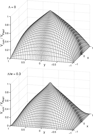
Figure 6: The ratio of the exact numerical interaction potential between two vortices and the Pearl interaction, $V_{\rm num}(x,y)/V_{\rm Pearl}(x,y)$, for a thin square of size $2w\times 2w$ with one vortex positioned at the square center ($0,0$) and the other vortex at $(x,y)$. Top: $\Lambda=0$. Bottom: $\Lambda=0.3w$.

VII Ratio of numerical and Pearl potentials

The analytical Pearl potential (19) (Fig. 5) does not depend on the shape of the film, in particular, it does not vanish at the outer and inner edges as it should. If an approximate analytic interaction potential is needed, e.g., for computer simulation of vortex motion and vortex pinning in films, one may construct this for simple film shapes like circular disks or rectangles or long strips, by multiplying the Pearl potential by a factor $f(x,y)$ that vanishes at the film edges with a $\Lambda$ dependent slope and that looks like a conical mountain whose maximum height for $\Lambda=0$ reaches unity and for $\Lambda>0$ is somewhat lower than unity. This numerical finding means that for $\Lambda>0$ the correct, shape-dependent interaction is smaller than the ideal Pearl potential. The physical reason for this is that for finite films the magnetic field lines of a vortex do not extend to infinity but return around the film edges, thereby reducing the sheet current that causes the vortex–vortex interaction, see discussion before Eq. (1).

Two examples for this factor $f(x,y)=V_{\rm num}(x,y)/V_{\rm Pearl}(x,y)$ , i.e., the ratio of the exact numerical potential and the ideal Pearl potential, are depicted in Fig. 6 for a superconducting thin film square with the first vortex positioned at the center ($0,0$) and the second vortex at $(x,y)$. This ratio has approximately conical shape, i.e., the correction factor $V_{\rm num}/V_{\rm Pearl}$ nearly linearly goes from unity to zero as the second vortex moves from the center to the edge of the square. It can be nicely seen in Fig. 6 that near the edges $V_{\rm num}(x,y)$ vanishes $\propto\delta^{1/2}$ when $\Lambda=0$ and $\propto\delta$ when $\Lambda>0$. These plots also show the somewhat unexpected result that the deviation of the exact interaction potential from the Pearl potential can be considerable even when both vortices are far from the film edges.

VIII Summary

It is shown that the interaction potential between two Pearl vortices in a superconducting thin infinite film can be well approximated by a simple logarithm at all distances, Eq. (6) and Fig. 1. A general argument is given why this interaction at large distances $r\gg\Lambda$ has the universal behavior $V(r)=\Phi_{0}^{2}/(\mu_{0}\pi r)$, independent of the 2D magnetic penetration depth $\Lambda=\lambda^{2}/d$. Explicit expressions are given for the interaction of one central Pearl vortex with an infinite regular lattice of pinned Pearl vortices or with the image vortices in numerical simulations that use periodic boundary conditions. The curvature of this interaction (spring constant of the central vortex) is presented both for this regular rigid lattice, and for the elastically deformable lattice of Pearl vortices. The modification of these results by the finite extension of the vortex lattice in finite films (e.g., disks) is given, see Fig. 2. Finally, it is shown how the interaction of the vortices in thin films of finite size and arbitrary shape can be computed. This general vortex–vortex interaction potential depends not only on the distance $r=|{\bf r}_{1}-{\bf r}_{2}|$ of the two Pearl-like vortices but on both positions ${\bf r}_{1}$ and ${\bf r}_{2}$. The interaction in general is not central; e.g., the interaction force on a vortex near the film edge acts perpendicular to this edge no matter where the other vortex is positioned. Anyway, this non-central interaction is caused by the other vortex and it vanishes when one of the two vortices approaches the edge. Examples for this correct interaction are shown in Figs. 3 and 4. Figure 5 shows the corresponding radial-symmetric and film-shape independent Pearl potential that, away from the film edges, exhibits the approximately correct peaks but does not vanish at the (inner and outer) film edges as the correct potential does. The correct numerical vortex interaction in finite-size films everywhere in the film is weaker than the ideal, infinite-film vortex interaction potential of Pearl, except when both vortices are close to each other near the middle of the film. This is shown in Fig. 6 for a square film with one vortex at the center.

Appendix A Elasticity theory

The linear elastic restoring force experienced by a displaced vortex in a 2D lattice of pinned or pin-free vortices may also be calculated from the theory of elasticity of the vortex lattice. Within this 2D problem the vortex lattice is described by its uniaxial compressional modulus $c_{11}$ and by its shear modulus $c_{66}$, which is typically much smaller, $c_{66}\ll c_{11}$. Within London theory one has for the triangular lattice of parallel Abrikosov vortices 10 ; 11 ; 12

$$c_{11}(k)={\bar{B}^{2}/\mu_{0}\over 1+k^{2}\lambda^{2}},~{}~{}c_{66}={\bar{B}\Phi_{0}\over 16\pi\mu_{0}\lambda^{2}}\,,$$ (20)

where ${\bf k}=(k_{x},k_{y})$ is the wave vector of the periodic displacement field. The $k$ dependence (dispersion) of $c_{11}(k)$ means that the elasticity is nonlocal. One has the ratio $c_{11}(0)/c_{66}=8b\kappa^{2}=(32\pi/\sqrt{3})(\lambda/a)^{2}\gg 1$, with $b=\bar{B}/B_{c2}$ and $B_{c2}=\Phi_{0}/(2\pi\xi^{2})$ the upper critical field of the superconductor. Expressions (A1) are valid when the magnetic fields of the vortices overlap, i.e., for vortex spacings $a\ll 2\pi\lambda$ equivalent to $1/(2\kappa^{2})\ll b\ll 1$. At very small inductions, approximate expressions may be obtained by considering only nearest neighbor interaction, yielding $c_{11}\propto c_{66}\propto\exp(-a/\lambda)$.

Interestingly, for the 2D lattice of Pearl vortices in thin films the same moduli $c_{11}$, $c_{66}$, Eq. (A1), apply (referred to unit volume). Namely, in the limit of thin films with thickness $d\ll\lambda$ in the London limit $\kappa\gg 1$ one has 5 for the moduli per unit area $dc_{11}(k)=d\bar{B}^{2}/(\mu_{0}k^{2}\lambda^{2})=\bar{B}^{2}/(\mu_{0}k^{2}\Lambda)$ (for $k^{2}\lambda^{2}\gg 1$) and $dc_{66}=\bar{B}\Phi_{0}/(16\pi\mu_{0}\Lambda)$. Thus, the below results apply both to the lattice of parallel Abrikosov vortices with length $d\gg a$ and to thin films with thickness $d\ll\lambda$.

We introduce the vortex displacements ${\bf u}_{\nu}={\bf u(R}_{\nu})$ and their Fourier transforms ${\bf u(k)}=[u_{x}({\bf k}),u_{y}({\bf k})]$,

$${\bf u}_{\nu}=\!\int_{\!BZ}{d^{2}k\over 4\pi^{2}}\,{\bf u(k)}\,e^{i{\bf kR_{\nu}}}\!,~{}{\bf u(k)}=\!\sum_{\nu}\!{{\bf u}_{\nu}\over n}\,e^{-i{\bf kR_{\nu}}}\!.$$ (21)

Here $n=\bar{B}/\Phi_{0}$ is the vortex density and the ${\bf k}$ integral is over the first Brillouin zone (BZ) with area $4\pi^{2}n=\pi k_{B}^{2}$, where $k_{B}=(4\pi n)^{1/2}\approx\pi/a$ is the radius of the circle that may be used to approximate the hexagonal BZ. At the maximum $k=k_{B}$ one has $c_{11}(k_{B})/c_{66}=4$. The elastic energy per unit area (hence the factor $d$) is

$$F_{\rm elast}={d\over 2}\!\int_{\!BZ}{d^{2}k\over 4\pi^{2}}\,u_{\alpha}({\bf k})\Phi_{\alpha\beta}({\bf k})u_{\beta}^{*}({\bf k})\,.$$ (22)

In it $\Phi_{\alpha\beta}({\bf k})$ with $\alpha,\beta=x,y$ is the elastic matrix, $\Phi_{\alpha\beta}({\bf k})=(c_{11}-c_{66})k_{\alpha}k_{\beta}+\delta_{\alpha\beta}c_{66}k^{2}$ with $k^{2}=k_{x}^{2}+k_{y}^{2}$. Explicitly one has

$$\Phi_{xx} = c_{11}k_{x}^{2}+c_{66}k_{y}^{2},~{}\Phi_{yy}=c_{66}k_{x}^{2}+c_{11}k_{y}^{2}\,$$

$$\Phi_{xy} = \Phi_{yx}=(c_{11}-c_{66})k_{x}k_{y}\,,$$ (23)

the determinant of $\Phi_{\alpha\beta}({\bf k})$ is $D({\bf k})=k^{4}c_{11}c_{66}$, and the inverse matrix has the elements $(\Phi^{-1})_{xx}=\Phi_{yy}/D$, $(\Phi^{-1})_{yy}=\Phi_{xx}/D$, and $(\Phi^{-1})_{xy}=(\Phi^{-1})_{yx}=\Phi_{xy}/D$. We shall now apply this formalism to two problems.

First, we consider the problem of Eq. (12): all vortices are rigidly pinned but the free vortex at the origin is shifted by a distance $u_{0}$ along $x$, thus ${\bf u}_{\nu}=u_{0}\delta_{\nu,0}{\bf\hat{x}}$. Inserting this into (A2) yields ${\bf u(k)}=(u_{0}/n){\bf\hat{x}}$ and the elastic energy (A3) becomes

$$F_{\rm elast}={u_{0}^{2}\over 2}\,V^{\prime\prime}_{c,\infty}(0)={d\over 2}\int_{\!BZ}{d^{2}k\over 4\pi^{2}}\,\Phi_{xx}({\bf k})\,{u_{0}^{2}\over n^{2}}\,.$$ (24)

Since $c_{11}\gg c_{66}$ one has from Eqs. (A1) and (A4) $\Phi_{xx}\approx c_{11}(k)k_{x}^{2}\approx(\bar{B}^{2}/\mu_{0})k_{x}^{2}/(1+k^{2}\lambda^{2})\approx(\bar{B}^{2}/\mu_{0}\lambda^{2})k_{x}^{2}/k^{2}$. Averaging $k_{x}^{2}/k^{2}=\cos^{2}\varphi$ over the angle $\varphi$ yields $1\over 2$. With the BZ area $4\pi^{2}n$ we thus obtain the potential curvature

$$V^{\prime\prime}_{c,\infty}(0)={\bar{B}^{2}d\over\mu_{0}\lambda^{2}n^{2}}\int_{\!BZ}{d^{2}k\over 4\pi^{2}}\,{k_{x}^{2}\over k^{2}}={\bar{B}\Phi_{0}d\over 2\mu_{0}\lambda^{2}}\,.$$ (25)

This coincides with Eq. (14).

Second, we consider the case when all vortices in a cylinder or disk with radius $R_{d}$ can move freely, only the vortices at the surface or edge $r=R_{d}$ are pinned to ensure zero displacement there. We calculate the elastic force $f_{0}$ that is required to move the central vortex a distance $u_{0}$, thereby deforming the vortex lattice. Thus, the applied forces on the vortices are all zero except for the force acting on the central vortex, ${\bf f}_{\nu}=f_{0}\delta_{\nu,0}{\bf\hat{x}}$. In general, we define the forces ${\bf f}_{\nu}$ per unit length (the total force on the $\nu$th vortex of length $d$ is $d{\bf f}_{\nu}$) and their Fourier transform ${\bf f(k)}=[f_{x}({\bf k}),f_{y}({\bf k})]$ by

$${\bf f}_{\nu}=\!\int_{\!BZ}{d^{2}k\over 4\pi^{2}}\,{\bf f(k)}\,e^{i{\bf kR_{\nu}}}\!,~{}{\bf f(k)}=\!\sum_{\nu}\!{{\bf f}_{\nu}\over n}\,e^{-i{\bf kR_{\nu}}}\!.$$ (26)

The elastic energy (A3) may also be written as

$$F_{\rm elast}\!\! = {d\over 2}\,\sum_{\nu}\,{\bf f}_{\nu}\,{\bf u}_{\nu}$$ (27)

$$= {d\over 2}\,n\int_{\!BZ}{d^{2}k\over 4\pi^{2}}\,f_{\alpha}({\bf k})\,u_{\alpha}^{*}({\bf k})$$

$$= {d\over 2}\,n^{2}\!\!\int_{\!BZ}{d^{2}k\over 4\pi^{2}}\,f_{\alpha}({\bf k})\,\Phi^{-1}_{\alpha\beta}({\bf k})f_{\beta}^{*}({\bf k})\,.$$

Displacements and forces are related by

$$nf_{\alpha}({\bf k})=\Phi_{\alpha\beta}({\bf k})u_{\beta}^{*}({\bf k})\,,$$

$$u_{\alpha}({\bf k})=n\Phi^{-1}_{\alpha\beta}({\bf k})f_{\beta}^{*}({\bf k})\,.$$ (28)

For our example ${\bf f}_{\nu}=f_{0}\delta_{\nu,0}{\bf\hat{x}}$ one has ${\bf f(k)}=(f_{0}/n){\bf\hat{x}}$ and the elastic energy becomes, with $\Phi^{-1}_{xx}\approx k_{y}^{2}/(k^{4}c_{66})$,

$$F_{\rm elast}={df_{0}^{2}\over 2}\!\int_{\!BZ}{d^{2}k\over 4\pi^{2}}\,\Phi_{xx}^{-1}({\bf k})={df_{0}^{2}\ln(R_{d}k_{B})\over 8\pi c_{66}}\,.$$ (29)

For the ${\bf k}$ integral we have used a lower cut-off $R_{d}^{-1}$ and the upper limit $k_{B}\approx\pi/a$. The curvature of the elastic potential, $V^{\prime\prime}_{\rm elast}(0)$, that the vortex at the origin feels is defined by

$$F_{\rm elast}={1\over 2}\,u_{0}^{2}V^{\prime\prime}_{\rm elast}(0)={1\over 2}\,{d^{2}f_{0}^{2}\over V^{\prime\prime}_{\rm elast}(0)}\,,$$ (30)

since the central force is $df_{0}=V^{\prime\prime}_{\rm elast}(0)u_{0}$, i.e., $V^{\prime\prime}_{\rm elast}(0)$ is a spring constant. Comparing Eqs. (A10) and (A11) and using the shear modulus (A1) we obtain

$$V^{\prime\prime}_{\rm elast}(0)={\bar{B}\,\Phi_{0}\,d\over 4\mu_{0}\lambda^{2}\ln(R_{d}k_{B})}={V^{\prime\prime}_{c,\infty}(0)\over 2\ln(\pi R_{d}/a)}\,.$$ (31)

Thus, when the surrounding vortices are allowed to relax elastically, the displacement of the central vortex, on which a force acts, is increased by a factor $2\ln(\pi R_{d}/a)$.

References

- (1) J. Pearl, Appl. Phys. Lett. 5, 65 (1964).
- (2) J.-C. Wei and T.-J. Yang, Jpn. J. Appl. Phys. 35, 5696 (1996).
- (3) D. Yu. Irz, V. N. Ryzhov, and E. E. Tareyeva, Phys. Lett. A 207, 374 (1995).
- (4) G. Carneiro and E. H. Brandt, Phys. Rev. B 61, 6370 (2000).
- (5) E. H. Brandt, Phys. Rev. B 71, 014521 (2005).
- (6) P. S. Deo, V. A. Schweigert, F. M. Peeters, and A. K. Geim, Phys. Rev. Lett. 79, 4653 (1997).
- (7) V. A. Schweigert and F. M. Peeters, Phys. Rev. Lett. 83, 2409 (1999).
- (8) V. A. Schweigert and F. M. Peeters, Physica C 332, 266, 426 (2000).
- (9) B. J. Baelus, L. R. E. Cabral, and F. M. Peeters, Phys. Rev. B 69, 064506 (2004).
- (10) D. S. Golubovic, M. V. Milošević, F. M. Peeters, and V. V. Moshchalkov, Phys. Rev. B 71, 180502(R) (2005).
- (11) V. R. Misko, B. Xu, and F. M. Peeters, Phys. Rev. B 76, 024516 (2007).
- (12) Guo-Qiao Zha, Shi-Ping Zhou, and Bao-He Zhu, Phys. Rev. B 73. 092512 (2006).
- (13) B. J. Baelus and F. M. Peeters, Phys. Rev. B 65, 104515 (2002).
- (14) G. R. Berdiyorov, B. J. Baelus, M. V. Milosevic, and F. M. Peeters, Phys. Rev. B 68, 174521 (2003).
- (15) G. R. Berdiyorov, M. V. Milošević, and F. M. Peeters, J. Low Temp. Phys. 139, 229 (2005).
- (16) B. J. Baelus, A. Kanda, N. Shimizu, K. Tadano, Y. Ootuka, K. Kadowaki, and F. M. Peeters, Phys. Rev. B 73, 024514 (2006).
- (17) A. V. Silhanek, W. Gillijns, A. Volodin, V. V. Moshchalkov, M. V. Milošević, and F. M. Peeters, Phys. Rev. B 76, 100502(R) (2007).
- (18) M. V. Milošević and F. M. Peeters, Phys. Rev. Lett. 93, 267006 (2004); Phys. Rev. B 68, 024509 (2003).
- (19) G. R. Berdiyorov, B. J. Baelus, M. V. Milošević, and F. M. Peeters, Phys. Rev. B 68, 174521 (2003).
- (20) G. R. Berdiyorov, M. V. Milošević, and F. M. Peeters, J. Low Temp. Phys. 139, 229 (2005).
- (21) M. V. Milošević, S. V. Yampolskii, and F. M. Peeters, Phys. Rev. B 66, 024515 (2002).
- (22) L. R. E. Cabral and F. M. Peeters, Phys. Rev. B 70, 214522 (2004).
- (23) A. D. Hernández and A. López, Phys. Rev. B 77, 144506 (2008).
- (24) E. Sardella, P. Noronha Lisboa Filho, and A. L. Malvezzi, Phys. Rev. B 77, 104508 (2008).
- (25) E. H. Brandt, Phys. Rev. B 64, 024505 (2001).
- (26) E. H. Brandt, Phys. Rev. B 72, 024529 (2005).
- (27) M. Abramowitz and I. A. Stegun, eds., Handbook of Mathematical Functions (National Bureau of Standards, Washington, 1967).
- (28) J. R. Clem, J. Superconductivity 17, 613 (2004). Note that Clem uses a different definition of .
- (29) E. H. Brandt, phys. stat.sol.(b) 77, 551 (1976).
- (30) E. H. Brandt, J. Low Temp. Phys. 26, 735, 709 (1977).
- (31) R. Labusch, phys. stat.sol. 32, 436 (1969).
- (32) J. R. Clem, J. Low Temp. Phys. 18, 427 (1975).
- (33) E. H. Brandt, Phys. Rev. Lett. 78, 2208 (1997).
- (34) A. Yaouanc, P. Dalmas de Réotier, and E. H. Brandt, Phys. Rev. B 55, 11107 (1997).
- (35) J. R. Clem and E. H. Brandt, Phys. Rev. B 72, 174511 (2005).
- (36) E. H. Brandt, J. de Physique 48, Colloque C8, 31-43 (1987).