Phase sensitive two mode squeezing and photon correlations from exciton superfluid

Abstract

There have been experimental and theoretical studies on Photoluminescence (PL) from possible exciton superfluid in semiconductor electron-hole bilayer systems. However, the PL contains no phase information and no photon correlations, so it can only lead to suggestive evidences. It is important to identify smoking gun experiments which can lead to convincing evidences. Here we study two mode phase sensitive squeezing spectrum and also two photon correlation functions. We find the emitted photons along all tilted directions are always in a two mode squeezed state between $\vec{k}$ and $-\vec{k}$. There are always two photon bunching, the photon statistics is super-Poissonian. Observing these unique features by possible future phase sensitive homodyne experiment and HanburyBrown-Twiss type of experiment could lead to conclusive evidences of exciton superfluid in these systems.

I Introduction

There have been extensive activities to study the superfluid of two species quantum degenerate fermionic gases across the BCS to BEC crossover tuned by the Feshbach resonances momfer ; vortexfer ; feshbach . The detection of a sharp peak in the momentum distribution of fermionic atom pairs gives a suggestive evidence of the superfluid momfer . However, the most convincing evidence comes from the phase sensitive observation of the vortex lattice across the whole BEC in BCS crossovervortexfer . In parallel to these achievements in the cold atoms, there have also been extensive experimental search of exciton superfluid loz in semiconductor $GaAs/AlGaAs$ electron-hole bilayer system (EHBL) butov ; field . Similar to the quantum degenerate fermionic gases, the EHBL also displays the BEC to BCS crossover tuned by the the density of excitons at a fixed interlayer distanceye . Several features of Photoluminescence (PL) butov suggest a possible formation of exciton superfluid at low temperature. There are also several theoretical work on the PL from the possible exciton superfluid phases angular ; spain ; power . Because the PL is a photon density measurement, it has the following serious limitations: (1) It can not detect the quantum nature of emitted photons. (2) It contains no phase information. (3) It contains no photon correlations. As first pointed out by Glauber glauber and others book1 , it is only in higher-order interference experiments involving the interference of photon quadratures or intensities which can distinguish the predictions between classical and quantum theory. So the evidence from the PL on possible exciton superfluid is only suggestive. Just like in the quantum degenerate fermionic gases, it is very important to perform a phase sensitive measurement that can provide a conclusive evidence for the possible exciton superfluid in EHBL. Unfortunately, it is technically impossible to rotate the EHBL to look for vortices or vortex lattices. In this paper, we show that the two mode phase sensitive measurement which is the interference of photon quadratures in Eqn.4 can provide such a conclusive evidence. We will also study the correlations of the photon intensities which is the interference of photon intensities in Eqn.11. We find that the two mode squeezing spectra and the two photon correlation functions between $\vec{k}$ and $-\vec{k}$ show unique, interesting and rich structures. The emitted photons along all tilted directions due to the quasi-particles above the condensate are in a two modes squeezed state between in-plane momentum $\vec{k}$ and $-\vec{k}$. From the two photon correlation functions, we find there are photon bunching, the photo-count statistics is super-Poissonian. These remarkable features can be used for high precision measurements and quantum information processing. We also discuses the possible future phase sensitive homodyne measurement to detect the two mode squeezing spectrum and the HanburyBrown-Twiss type of experiments to detect two photon correlations. Observing these unique features by these experiments could lead to conclusive evidences of exciton superfluid in these systems.

The rest of the paper is organized as follows. In Section II, we present the photon-exciton interaction Hamiltonian and the input-output relation between incoming and outgoing photons. Then we apply the input-output formalism to study the two mode squeezing between the photons at $\vec{k}$ and $-\vec{k}$. in section III and the two photon correlations and photon statistics in Section IV. We reach conclusions in Sect.V and also present some future open problems.

II The Photon-exciton interaction and Input-out formalism

The total Hamiltonian is the sum of excitonic superfluid part, photon part and the coupling between the two parts $H_{t}=H_{sf}+H_{ph}+H_{int}$ where :

$$H_{sf} = \sum_{\vec{k}}(E_{\vec{k}}^{ex}-\mu)b_{\vec{k}}^{\dagger}b_{\vec{k}}+\frac{1}{2A}\sum_{\vec{k}\vec{p}\vec{q}}V_{d}(q)b_{\vec{k}-\vec{q}}^{\dagger}b_{\vec{p}+\vec{q}}^{\dagger}b_{\vec{p}}b_{\vec{k}}$$

$$H_{ph} = \sum_{k}\omega_{k}a_{k}^{\dagger}a_{k},~{}~{}~{}~{}H_{int}=\sum_{k}[ig(k)a_{k}b_{\vec{k}}^{\dagger}+h.c.]$$ (1)

where $A$ is the area of the EHBL, the exciton energy $E_{\vec{k}}^{ex}=\vec{k}^{2}/2M+E_{g}-E_{b}$, the photon frequency $\omega_{k}=v_{g}\sqrt{k_{z}^{2}+\vec{k}^{2}}$ where $v_{g}=c/\sqrt{\epsilon}$ with $c$ the light speed in the vacuum and $\epsilon\sim 12$ the dielectric constant of $GaAs$, $k=(\vec{k},k_{z})$ is the 3 dimensional momentum, $V_{d}(\vec{q})$ is the dipole-dipole interaction between the excitons ye , $V_{d}(\left|\vec{r}\right|\gg d)=e^{2}d^{2}/\left|\vec{r}\right|^{3}$ and $V_{d}(q=0)=\frac{2\pi e^{2}d}{\epsilon}$ where $d$ is the interlayer distance leads to a capacitive term for the density fluctuation psdw . The $g(k)\sim\vec{\epsilon}_{k\lambda}\cdot\vec{D}_{k}\times L^{-1/2}_{z}$ is the coupling between the exciton and the photons where $\vec{\epsilon}_{k\lambda}$ is the photon polarization, $\vec{D}_{k}$ is the transition dipole moment and $L_{z}\rightarrow\infty$ is the normalization length along the $z$ direction power . As emphasized in power , the effect of off-resonant pumping in the experiments in butov is just keep the chemical potential $\mu$ in Eqn.1 a constant in a stationary state.

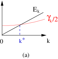
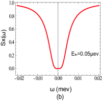
Figure 1: (a) The energy spectrum and the decay rate of the exciton versus in-plane momentum $\vec{k}$ of an exciton superfluid. (b) The squeezing spectrum at a given in-plane momentum $\vec{k}$ when $E(\vec{k})<\gamma_{\vec{k}}/2$. The $nV_{d}(\vec{k})$ and $\gamma_{\vec{k}}/2$ are fixed at $50\mu eV$ and $0.1\mu eV$ respectively as used in power . They are also used in all the following figures. There exists only one minimal when the photon frequency equals to the chemical potential with the width $\delta_{1}(\vec{k})$ given in the text. Near the resonance, the squeezing ratio is so close to zero that it can not be distinguished in the figure.

We can apply standard Bogoloubov approximation to this system. We decompose the exciton operator into the condensation part and the quantum fluctuation part above the condensation $b_{\vec{k}}=\sqrt{N}\delta_{\vec{k}0}+\tilde{b}_{\vec{k}}$. The excitation spectrum is given by $E(\vec{k})=\sqrt{\epsilon_{\vec{k}}[\epsilon_{\vec{k}}+2\bar{n}V_{d}(\vec{k})]}$ whose $\vec{k}\rightarrow 0$ behavior is shown in Fig.1a. We also decompose the interaction Hamiltonian $H_{int}$ in Eqn.1 into the coupling to the condensate part $H_{int}^{c}=\sum_{k_{z}}[ig(k_{z})(\sqrt{N}+\tilde{b}_{0})a_{k_{z}}+h.c.]$ and to the quasi-particle part $H_{int}^{q}=\sum_{k}[ig(k)a_{k}\tilde{b}_{\vec{k}}^{\dagger}+h.c.]$. The $\vec{k}=0$ part was analyzed in power . In this paper, we focus on the two mode squeezing spectrum and the two photon correlations between $\vec{k}$ and $-\vec{k}$. The output field $a_{\vec{k}}^{out}(\omega)$ is related to the input field by online :

$$a_{\vec{k}}^{out}(\omega) = [-1+\gamma_{\vec{k}}G_{n}(\vec{k},\omega+i\frac{\gamma_{k}}{2})]a_{\vec{k}}^{in}(\omega)$$ (2)

$$+\gamma_{\vec{k}}G_{a}(\vec{k},\omega+i\frac{\gamma_{k}}{2})a_{-\vec{k}}^{in\dagger}(-\omega),$$

where the normal Green function $G_{n}(\vec{k},\omega)=i\frac{\omega+\epsilon_{\vec{k}}+\bar{n}V_{d}(\vec{k})}{\omega^{2}-E^{2}(\vec{k})}$ and the anomalous Green function $G_{a}(\vec{k},\omega)=\frac{i\bar{n}V_{d}(\vec{k})}{\omega^{2}-E^{2}(\vec{k})}$ with $\omega=\omega_{k}-\mu$ power . The exciton decay rate in the two Green functions are $\gamma_{\vec{k}}=D_{\vec{k}}(\mu)\left|g_{\vec{k}}(\omega_{k}=\mu)\right|^{2}$ which is independent of $L_{z}$ power , so is an experimentally measurable quantity. Just from the rotational invariance, we can conclude that $\gamma_{\vec{k}}\sim const.+|\vec{k}|^{2}$ as $\vec{k}\rightarrow 0$ as shown in Fig.1a.

III The two modes squeezing between $\vec{k}$ and $-\vec{k}$.

Eqn.2 suggests that it is convenient to define $A_{\vec{k},\pm}^{out}(\omega)=[a_{\vec{k}}^{out}(\omega)\pm a_{-\vec{k}}^{out}(\omega)]/\sqrt{2}$ and $A_{\vec{k},\pm}^{in}(\omega)=[a_{\vec{k}}^{in}(\omega)\pm a_{-\vec{k}}^{in}(\omega)]/\sqrt{2}$. Then the position and momentum ( quadrature phase ) operators of the output field can be defined by:

$$X_{\pm} = A_{\vec{k},\pm}^{out}(\omega)e^{i\phi_{\pm}(\omega)}+A_{\vec{k},\pm}^{out\dagger}(-\omega)e^{-i\phi_{\pm}(-\omega)}$$

$$iY_{\pm} = A_{\vec{k},\pm}^{out}(\omega)e^{i\phi_{\pm}(\omega)}-A_{\vec{k},\pm}^{out\dagger}(-\omega)e^{-i\phi_{\pm}(-\omega)}$$ (3)

The squeezing spectra book1 which measure the fluctuation of the canonical position and momentum are defined by

$$S_{X_{\pm}}(\omega) = \left\langle X_{\pm}(\omega)X_{\pm}(-\omega)\right\rangle_{in}$$

$$S_{Y_{\pm}}(\omega) = \left\langle Y_{\pm}(\omega)Y_{\pm}(-\omega)\right\rangle_{in}.$$ (4)

where the in-state is the initial zero photon state $|in\rangle=|BEC\rangle|0\rangle$. For notational conveniences, we set $\phi_{-}(\omega)=\pi/2+\phi_{+}(\omega)$ and just set $\phi_{+}(\omega)\equiv\phi(\omega)$. Then we find $S_{X_{+}}(\omega)=S_{X_{-}}(\omega)=S_{X}(\omega)$ and $S_{Y_{+}}(\omega)=S_{Y_{-}}(\omega)=S_{Y}(\omega)$. The phase $\phi(\omega)$ is chosen to achieve the largest possible squeezing, namely, by setting $\partial S_{X}(\omega)/\partial\omega=0$ which leads to:

$$\cos 2\phi(\omega)=\frac{\gamma_{\vec{k}}(\epsilon_{\vec{k}}+\bar{n}V_{d}(\vec{k}))}{\sqrt{\Omega^{2}(\omega)+\gamma_{\vec{k}}^{2}E^{2}(\vec{k})+(\bar{n}V_{d}(\vec{k})\gamma_{\vec{k}})^{2}}},$$ (5)

where $\Omega(\omega)=\omega^{2}-E^{2}(\vec{k})+\gamma_{\vec{k}}^{2}/4$.

Substituting Eqns.2 and 3 into Eq.4 leads to

$$S_{X}(\omega) = 1-\frac{2\gamma_{\vec{k}}\bar{n}V_{d}(\vec{k})}{\mathcal{N}(\omega)+\gamma_{\vec{k}}\bar{n}V_{d}(\vec{k})}$$

$$S_{Y}(\omega) = 1+\frac{2\gamma_{\vec{k}}\bar{n}V_{d}(\vec{k})}{\mathcal{N}(\omega)-\gamma_{\vec{k}}\bar{n}V_{d}(\vec{k})}$$ (6)

where $\mathcal{N}(\omega)=\sqrt{\Omega^{2}(\omega)+\gamma_{\vec{k}}^{2}E^{2}(\vec{k})+(\bar{n}V_{d}(\vec{k})\gamma_{\vec{k}})^{2}}$. This equation leads to:

$$S_{X}(\omega)S_{Y}(\omega)=1.$$ (7)

which shows that for a given in-plane momentum $\vec{k}$ and a given photon frequency $\omega=\omega_{k}-\mu$, there always exists a two mode squeezing state which can be decomposed into two squeezed states along two normal angles: one squeezed along the angle $\phi(\omega)$ and the other along the angle $\phi(\omega)+\pi/2$ in the quadrature phase space ($X,Y$). Now we discuss the over-damping $k<k^{\ast},E(\vec{k})<\gamma_{\vec{k}}/2$ case and the under-damping $k>k^{\ast},E(\vec{k})>\gamma_{\vec{k}}/2$ case respectively.

(1) Low momentum regime $|\vec{k}|<k^{\ast}$: $E(\vec{k})<\gamma_{\vec{k}}/2$.

From Eqn.6, we can see that the maximum squeezing happens at $\omega_{\min}=0$ which means at $\omega_{k}=\mu$:

$$S_{X}(\vec{k},\omega=0) = 1-\frac{2\gamma_{\vec{k}}\bar{n}V_{d}(\vec{k})}{\mathcal{N}(0)+\bar{n}V_{d}(\vec{k})\gamma_{\vec{k}}}$$

$$\cos 2\phi(\vec{k},\omega=0) = \frac{\gamma_{\vec{k}}(\epsilon_{\vec{k}}+\bar{n}V_{d}(\vec{k}))}{\mathcal{N}(0)}$$ (8)

where $\mathcal{N}(0)\equiv\mathcal{N}(\omega=0)=\sqrt{[E^{2}(\vec{k})+\gamma_{\vec{k}}^{2}/4]^{2}+(\bar{n}V_{d}(\vec{k})\gamma_{\vec{k}})^{2}}$which is defined below Eqn.6. In sharp contrast to the large momentum regime $E(\vec{k})>\gamma_{\vec{k}}/2$ to be discussed in the following, the resonance position $\omega_{k}=\mu$ is independent of the value of $\vec{k}$, this is because the quasiparticle is not even well defined in the low momentum regimepower . The $\omega$ dependence of $S_{X}(\omega)$ in Eqn.6 is drawn in Fig.1b. The line width of the single peak in Fig.1b is $\delta_{1}(\vec{k})=2\sqrt{E^{2}(\vec{k})-\frac{\gamma_{\vec{k}}^{2}}{4}+O_{\vec{k}}}$ where $O_{\vec{k}}=\sqrt{4\mathcal{N}(0)[\mathcal{N}(0)+\bar{n}V_{d}(\vec{k})\gamma_{\vec{k}}]-\gamma_{\vec{k}}^{2}E^{2}(\vec{k})}$.

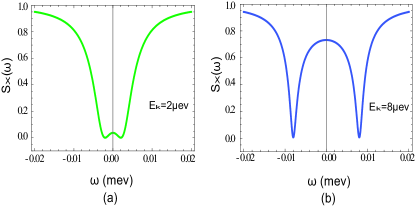
Figure 2: The squeezing spectrum at a given in-plane momentum $\vec{k}$ when $E(\vec{k})>\gamma_{\vec{k}}/2$. There exist two minima in the spectrum when the photon frequency resonate with the well defined quasi-particles. Near the resonance, the squeezing ratio is so close to zero that it can not be distinguished in the figure. (a) When $E(\vec{k})=2\mu eV$, the two peaks are still not clearly separated. (b) When $E(\vec{k})=8\mu eV\gg\gamma_{\vec{k}}/2$, the quasi-particles are well defined which lead to the two well defined resonances with the width $\delta_{2}(\vec{k})$ given in the text.

(2) Large momentum regime $k>k^{\ast}$: $E(\vec{k})>\gamma_{\vec{k}}/2$.

From Eqn.6, we can see that the maximum squeezing happens at the two resonance frequencies $\omega_{k}=\mu\pm[E^{2}(\vec{k})-\gamma_{\vec{k}}^{2}/4]^{1/2}$ where

$$S_{X}(\vec{k},\omega_{\min}) = (\frac{\epsilon_{\vec{k}}}{E(\vec{k})})^{2}=\frac{\hbar k^{2}}{\hbar^{2}k^{2}+4M\bar{n}V_{d}(\vec{k})}$$

$$\cos 2\phi(\vec{k},\omega_{\min}) = 1$$ (9)

In this case, $\phi(\vec{k},\omega_{\min})=0$. In sharp contrast to the low momentum regime discussed above, the resonance positions depend on $E(\vec{k})$, this is because the quasiparticle is well defined in the large momentum regime only power . From Eqn.9, we can see that increasing the exciton mass, the density, especially the exciton dipole-dipole interaction will all benefit the squeezing at the two resonances.

The $\omega$ dependence of $S_{X}(\omega)$ in Eqn.6 is drawn in Fig.2. When $E(\vec{k})>(Q_{\vec{k}}+\sqrt{1+Q_{\vec{k}}})\gamma_{\vec{k}}/2$, the line width of the each peak in Fig.2 is $\delta_{2}(\vec{k})=\sqrt{E^{2}(\vec{k})-\frac{\gamma_{\vec{k}}^{2}}{4}+\gamma_{\vec{k}}Q_{\vec{k}}E(\vec{k})}-\sqrt{E^{2}(\vec{k})-\frac{\gamma_{\vec{k}}^{2}}{4}-\gamma_{\vec{k}}Q_{\vec{k}}E(\vec{k})}$ where $Q_{\vec{k}}=\sqrt{3+\frac{4\bar{n}V_{d}(\vec{k})}{\epsilon_{\vec{k}}}}$. It is easy to see that $\delta_{2}\sim\gamma_{\vec{k}}Q_{\vec{k}}$ which is equal to the exciton decay rate $\gamma_{\vec{k}}$ multiplied by a prefactor $Q_{\vec{k}}$. When $E(\vec{k})<(Q_{\vec{k}}+\sqrt{1+Q_{\vec{k}}})\gamma_{\vec{k}}/2$, the two peaks are too close to be distinguished. It is important to observe that the two widths $\delta_{1}(\vec{k})$ and $\delta_{2}(\vec{k})$ not only depend on $\gamma_{\vec{k}}$, but also the interaction $\bar{n}V_{d}(\vec{k})$. This is in sharp contrast to the widths in the ARPS and EDC inpower which only depend on $\gamma_{\vec{k}}$.

The angle dependence of both $E(\vec{k})>\gamma_{\vec{k}}/2$ and $E(\vec{k})<\gamma_{\vec{k}}/2$ are drawn in the same plot Fig.3a for comparison. Both the squeezing spectrum in Eqn.6 and the rotated phase $\phi$ in Eqn.5 can be measured by phase sensitive homodyne detections book1 .

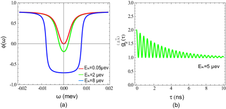
Figure 3: (a) The squeezing angle dependence on the frequency when $E(\vec{k})<\gamma_{\vec{k}}/2$ corresponding to Fig.1b and $E(\vec{k})>\gamma_{\vec{k}}/2$ corresponding to Fig.2a,2b. When $E(\vec{k})<\gamma_{\vec{k}}/2$ the squeezing angle is always non-zero. Near the resonance, the angle is so close to zero that it can not be distinguished in the figure. Only when $E(\vec{k})>\gamma_{\vec{k}}/2$ and the photon frequency resonate with the well defined quasi-particles, the squeezing angle is zero. Away from the resonance, the angle becomes negative. (b)The two photon correlation functions between $\vec{k}$ and $-\vec{k}$ against the delay time $\tau$.

IV The two photons correlation functions and photon statistics.

The quantum statistic properties of emitted photons can be extracted from two photon correlation functionsglauber . The normalized second order correlation functions of the output field for the two modes at $\vec{k}$ and $-\vec{k}$ are

$$g_{2}^{(\vec{k})}(\tau)=\frac{\left\langle a_{\vec{k}}^{out\dagger}(t)a_{\vec{k}}^{out\dagger}(t+\tau)a_{\vec{k}}^{out}(t+\tau)a_{\vec{k}}^{out}(t)\right\rangle_{in}}{\left|G_{1}(0)\right|^{2}}$$ (10)

and

$$g_{2}^{(\pm\vec{k})}(\tau)=\frac{\left\langle a_{\vec{k}}^{out\dagger}(t+\tau)a_{\vec{k}}^{out}(t+\tau)a_{-\vec{k}}^{out\dagger}(t)a_{-\vec{k}}^{out}(t)\right\rangle_{in}}{\left|G_{1}(0)\right|^{2}}$$ (11)

where the $G_{1}(\tau)=\langle a_{\vec{k}}^{out\dagger}(t+\tau)a_{\vec{k}}^{out}(t)\rangle_{in}$ is the single photon correlation function power . The second order correlation function $g_{2}^{(\pm\vec{k})}(\tau)$ determines the probability of detecting $n_{-\vec{k}}$ photons with momentum $-\vec{k}$ at time $t$ and detecting $n_{\vec{k}}$ photons with momentum $\vec{k}$ at time $t+\tau$. By using Eqn.2, we find

$$g_{2}^{(\vec{k})}(\tau) = 1+e^{-\gamma_{\vec{k}}\tau}[\cos(E(\vec{k})\tau)+\frac{\gamma_{\vec{k}}}{2E(\vec{k})}\sin(E(\vec{k})\tau)]^{2}$$

$$g_{2}^{(\pm\vec{k})}(\tau) = g_{2}^{(\vec{k})}(\tau)+e^{-\gamma_{\vec{k}}\tau}\frac{E^{2}(\vec{k})+\frac{\gamma_{\vec{k}}^{2}}{4}}{\bar{n}^{2}V_{d}^{2}(k)}$$ (12)

It turns out that the second correlation functions are independent of the relation between $E(\vec{k})$ and $\gamma_{\vec{k}}/2$. We only draw $g_{2}^{(\pm\vec{k})}(\tau)$ in the Fig.3b. When $\tau=0$ the two photon correlation function are $g_{2}^{(\vec{k})}(0)=2$, so just the mode $\vec{k}$ alone behaves like a chaotic light. This is expected because the entanglement is only between $-\vec{k}$ and $\vec{k}$. In fact, $g_{2}^{(\pm k)}(0)=2+\frac{E^{2}(\vec{k})+\frac{\gamma_{\vec{k}}^{2}}{4}}{\bar{n}^{2}V_{d}^{2}(\vec{k})}>g_{2}^{(\vec{k})}(0)=2$. So it violates the classical Cauchy-Schwarz inequality book1 which is completely due to the quantum nature of the two mode squeezing between $\vec{k}$ and $-\vec{k}$.

From Fig.3b, we can see that the two photon correlation function decrease as time interval $\tau$ increases which suggests quantum nature of the emitted photons is photon bunching and the photo-count statistics is super-Poissonian. It is easy to see that the envelope decaying function is given by the exciton decay rate $\gamma_{\vec{k}}$ shown in Fig.1b, while the oscillation within the envelope function is given by the Bogoliubov quasi-particle energy $E(\vec{k})$ shown also in Fig.1b. The $g_{2}^{(\pm\vec{k})}(\tau)$ can be measured by HanburyBrown-Twiss type of experiment book1 where one can extract both $E(\vec{k})$ and $\gamma_{\vec{k}}$.

V Conclusions and Perspectives

In conventional non-linear quantum optics, the generation of squeezed lights requires an action of a strong classical pump and a large non-linear susceptibility $\chi^{(2)}$. The first observation of squeezed lights was achieved in non-degenerate four-wave mixing in atomic sodium in 1985 fourwave . Here in EHBL, the generation of the two mode squeezed photon is due to a complete different and new mechanism: the anomalous Green function of Bogoliubov quasiparticle which is non-zero only in the excitonic superfluid state. The very important two mode squeezing result Eqn.7 is robust against any microscopic details such as the interlayer distance $d$, exciton density $\bar{n}$, exciton dipole-dipole interaction $V_{d}(q)$ and the exciton decay rate $\gamma_{\vec{k}}$. The applications of the squeezed state include (1) the very high precision measurement by using the quadrature with reduced quantum fluctuations such as the $X$ quadrature in the Fig.1b and Fig.2 where the squeeze factor reaches very close to $0$ at the resonances (2) the non-local quantum entanglement between the two twin photons at $\vec{k}$ and $-\vec{k}$ can be useful for many quantum information processes. (3) detection of possible gravitational waves grav . All these various salient features of the phase sensitive two mode squeezing spectra and the two photon correlation functions along normal and titled directions studied in this paper can map out completely and unambiguously the nature of quantum phases of excitons in EHBL such as the ground state and the quasi-particle excitations above the ground state. Both the squeezing spectrum in Fig.1b, Fig.2 and the rotated phase $\phi$ in Fig.3a can be measured by phase sensitive homodyne detections. The two photon correlation functions in Fig.3b can be measured by HanburyBrown-Twiss type of experiments. It is important to perform these these new experiments in the future to search for the most convincing evidences for the existence of exciton superfluid in the EHBL. The results achieved in this paper should also shed lights on how photons interact with cold atoms momfer ; vortexfer ; feshbach .

It was well known that a 2D superfluid at any finite temperature was given by the Kosterlitz-Thouless (KT) physics. Namely, at any non-zero temperature, there is no real BEC ( no real symmetry breaking ), only algebraic order where the correlation function decays algebraically. But the gapless superfluid mode with a finite superfluid density survives at finite temperatures upto the KT transition temperature. So the the condensate at $\vec{k}=0$ at $T=0$ will disappear at any finite $T$, so the properties of the photons emitted along the normal direction at $T=0$ studied in Ref. 10 need to be re-investigated at any finite $T$. This manuscript focused on the interaction between the photons and the Bogoliubov mode at tilted directions $\vec{k}\neq 0$, because the Bogoliubov mode is just the gapless superfluid mode which survives at finite temperatures until to the KT transition temperature, so we expect the results achieved in this manuscript will also survive at finite temperatures. How it will change near the KT transition temperature is an open problem to be discussed in a future publication. In all the experiments butov , the excitons are confined inside a trap , so there still could be a real BEC at finite temperature inside a trap. So the effects of trap also will also be investigated in a future publication.

ACKNOWLEDGEMENTS

We are very grateful for C. P. Sun for very helpful discussions and encouragements throughout the preparation through this manuscript. J. Ye’s research at KITP was supported in part by the NSF under grant No. PHY-0551164, at KITP-C was supported by the Project of Knowledge Innovation Program (PKIP) of Chinese Academy of Sciences. J.Ye thank Fuchun Zhang, Jason Ho, A. V. Balatsky, Jiangqian You, Yan Chen and Han Pu for their hospitalities during his visit at Hong Kong university, Ohio State university, LANL, Fudan university and Rice university.

References

- (1) C. A. Regal, M. Greiner, and D. S. Jin, Phys. Rev. Lett. 92, 040403 (2004).
- (2) M. W. Zwierlein, J. R. Abo-Shaeer, A. Schirotzek, C. H. Schunck, W. Ketterle, NATURE, 435, 1047 (2005).
- (3) For reviews, see Cheng Chin, Rudolf Grimm, Paul Julienne, Eite Tiesinga, arXiv:0812.1496.
- (4) Yu. E. Lozovik and V. I. Yudson, Pis’ma Zh. Eksp. Teor. Fiz. 22, 556 (1975) [JETP Lett. 22, 274 (1975)]
- (5) L. V. Butov, et al, Nature 417, 47 - 52 (2002); Nature 418, 751 - 754 (2002); C. W. Lai, et al Science 303, 503-506 (2004). D. Snoke, et al Nature 418, 754 - 757, 2002; D. Snoke, Nature 443, 403 - 404 (2006). R. Rapaport, et al, Phys. Rev. Lett. 92, 117405 (2004); Phys. Rev. B 72, 075428 (2005).
- (6) U. Sivan, P. M. Solomon, and H. Shtrikman, Phys. Rev. Lett. 68, 1196 - 1199 (1992). J. A. Seamons, D. R. Tibbetts, J. L. Reno, M. P. Lilly, Appl. Phys. Lett., 90, 052103, (2007).
- (7) Jinwu Ye, Jour. of Low Temp. Phys: 158, 882, (2010).
- (8) A. Olaya-Castro, F. J. Rodr guez, L. Quiroga, and C. Tejedor, Phys. Rev. Lett. 87, 246403 (2001).
- (9) Jonathan Keeling, L. S. Levitov, and P. B. Littlewood, Phys. Rev. Lett. 92, 176402 (2004).
- (10) Jinwu Ye, T. Shi and Longhua Jiang, Phys. Rev. Lett. 103, 177401 (2009).
- (11) R. J. Glauber, Phys. Rev. 130, 2529 (1963).
- (12) D. F. Walls and G. J. Milburn, Quantum Optics, Springer-Verlag, 1994.
- (13) Jinwu Ye and Longhua Jiang, Phys. Rev. Lett. 98, 236802 (2007), Jinwu Ye, Phys. Rev. Lett. 97, 236803 (2006). Jinwu Ye, Annals of Physics, 323 (2008), 580-630.
- (14) See EPAPS Document No. E-PRLTAO-103-002946 for the derivation of this input-output relation.
- (15) R. E. Slusher, et al Phys. Rev. Lett. 55, 2409 - 2412 (1985).
- (16) For recent development, see K. Goda, et al Nature Physics 4, 472 - 476 (2008).