University of Torino
Department of General Physics
Ph.D. Thesis in Astrophysics
 

Numerical approaches
to star formation and SuperNovae energy feedback
in simulations of galaxy clusters
 
Author: Martina Giovalli Supervisors:
Prof. Antonaldo Diaferio
Dr. Giuseppe Murante

Introduction

If a century ago, Astronomy concerned almost completely the description of the dynamics of objects that we could see, the situation has now reversed, with most of the astronomers more interested in how a certain observed situation might have come to be. To this end, numerical techniques have become standard tools for studying a wide range of cosmological and astrophysical problems.

Among the many open issues in modern Astronomy, galaxy formation is certainly one of the most important and studied. The physics of gravity only, which rules the formation and evolution of the large scale structure of the universe in a Cold Dark Matter cosmology, is sufficient to explain a number of relevant observations, ranging from the Cosmic Microwave Background Radiation power spectrum to the statistical properties of the distribution of galaxy and galaxy cluster. On the other hand, observed properties of galaxies (e.g. morphologies, luminosities, colours, stellar ages, Tully-Fisher relation), both in clusters and isolated galaxies, are not satisfactorily accounted for without considering a number of other astrophysical processes, in addition to the already complex interaction of nonlinear gravitational evolution and dissipative gas dynamics.

Observed cluster of galaxies are, in fact, composed by three main distinct components, dark matter, diffuse gas and stars, which have a completely different physics behind. Numerical codes following both dark matter and baryonic particles are now commonly used, but they still have shortcomings, mainly for two reasons. The first one is the enormous resolution needed, for example, to simultaneously follow the birth of stars and the Inter-Stellar Medium physics, and the large scale physics responsible for structure formation. The second one deals with the complexity of the involved physics. For example, the physics of the Inter-Stellar Medium (ISM) and the related star formation and energy feedback processes are currently not understood in full detail.

To deal with such problems, numerical simulation codes often resort to simplified, sub-grid models of the complex hydrodynamical and astrophysical processes working at scales where star formation takes place. Even then, detailed and satisfactory numerical models of galaxy formation and evolution, which starts from the formation of cosmic structures and self-consistently includes gas dynamics, star formation, SuperNovae (SNe) energy feedback and all the pertinent processes are still lacking.
Therefore, it is of paramount importance to improve the sub-grid treatment of the ISM physics in numerical simulation, paying particular attention to the feedback processes that arise from the energetic activity of massive dying stars, and taking place through winds, ionising photons and SNe explosions followed by the creation and propagation of hot expanding pressure fronts (SNe super-bubbles). This energy input is, in fact, believed to be the fundamental mechanism which shapes and sustains the Inter-Galactic Medium, thus preventing the “cooling catastrophe” typically found in Cold Dark Matter cosmologies and producing global galactic winds and “fountains” which can be observed in the real Universe. Finally, such an energy provides a source of heating for the Intra Cluster Medium, especially at the centre of established cooling flows, whose importance in the global galaxy cluster energy budget has to be carefully estimated.

The aim of this Thesis is thus to investigate different numerical approaches and to introduce a new, physically-based sub-grid model for the ISM physics, including a treatment of star formation and Type II supernovae energy feedback (MUPPI, MUlti-Phase Particle Integrator). Our model follows the ISM physics using a system of ordinary differential equations, describing mass and energy flows among the different gas phases in the ISM inside each gas particle. The model also includes the treatment of SNe energy transfer from star-forming particles to their neighbours. We will show in this Thesis how this model is able to reproduce observed ISM properties, while also providing an effective thermal energy feedback and responding to variations in the local hydrodynamical properties of the gas, e.g. crossing of a spiral density wave in a galaxy disk.

This thesis work is organised as follows:

Chapter 1

we provide the basics of the cosmological framework upon which this thesis is based. We begin by introducing the Hot Big-Bang theory and the theory of structure formation. We then pose particular attention on describing some of the observed physical properties of galaxy clusters, among which the diffuse stellar light. We finally introduce some open questions (and some possible answers) which are still unresolved in this field of Astronomy, focusing our attention on the role covered by supernovae feedback.

Chapter 2

we provide a review on existing star formation and supernovae feedback models. We first describe the numerical code GADGET 2, in which we implemented our novel algorithm MUPPI (Chapter 4). After reviewing the more relevant star formation models existing in literature, we describe the analytical model for the ISM by Monaco 2004, upon which MUPPI is based.

Chapter 3

we present our published results on the study of the formation mechanism of the diffuse stellar component in a cosmological hydrodynamical simulation. After describing the numerical simulations and the techniques for galaxy identification we use, we present the link between galaxy histories and the formation of the diffuse light. Finally, we discuss the dynamical mechanisms that unbind stars from galaxies in clusters and compare with the statistical analysis of the cosmological simulation we performed. We performed such work using the effective model for star formation and feedback (Springel & Hernquist 2003).

Chapter 4

we present the novel algorithm for the Interstellar Medium evolution, MUPPI (MUltiPhase Particle Integrator), whose implementation in GADGET2 has been the principal work of the present PhD thesis. We first describe how the model is initialised; then we give details on the model core and on all the processes regulating the evolution of the Interstellar Medium; finally, we account for the supernova energy redistribution from star-forming gas particles to their neighbours. In two appendices, we show the flow charts of MUPPI model and of GADGET-2 code.

Chapter 5

we present and discuss the results we obtained by using MUPPI with our reference set of parameters in various initial physical conditions, i.e. an isolated model of the Milky-Way, a model of a typical dwarf galaxy and two isolated non-rotating cooling-flow halos, equivalent to those used for the Milky-Way and the dwarf-like galaxy, but not containing any galaxy. Finally we show our test on the behaviour of MUPPI when we change numerical resolution and the most important model parameters.

Chapter 1 Basics of the cosmological framework

The evolution of the world can be compared to a display of fireworks that has just ended; some few red wisps, ashes and smoke. Standing on a cooled cinder, we see the slow fading of the suns, and we try to recall the vanishing brilliance of the origin of the worlds.’ Lemaître.

During last century, two observative discoveries have revolutionised our view of the Universe: the Expansion of the Universe in 1929 by Edwin Hubble and the Cosmic Microwave background in 1965 by Arno Penzias and Robert Wilson.
A relevant implication of the Hubble discovery is the formulation of the Cosmological Principle, which states that “On sufficiently large scales the Universe is both homogeneous and isotropic”, namely there are no special directions and no special places in the Universe. Since little was known empirically about the distribution of matter in the Universe, Einstein thought that the only way to put theoretical cosmology on a firm footing was to assume there was a basic simplicity to the global structure of the Universe enabling a similar simplicity in the local behaviour of matter. So first cosmologists had to content themselves with the construction of simplified models based on the guiding Cosmological Principle, with the hope of describing some general aspects of the Universe.
Since the Hubble discovery, many cosmological models have been proposed to describe the birth and evolution of the Universe. In the early 1960, there were mainly two rival theories of cosmogony: the Big Bang theory, which proposes that the universe was created in a giant explosion, and the Steady-state theory, which denies any beginning or end, being the Universe infinite and matter within it continuously created. The debate between these two philosophically opposite ideas, was over in 1965 with the detection of the Cosmic Microwave Background (CAB) radiation. The Big Bang theory was the clear winner for the simple reason that the steady-state model did not predict and could not reasonably account for the presence of the cosmic background radiation. On the other side, the Big Bang theory not only predicted the background radiation but required it.
Thanks to the remarkable progresses achieved by cosmological observations, the formulation of cosmological models became much more reliable. Our current knowledge of the birth and evolution of the Universe and of the objects it contains is based on the Hot Big-Bang theory, or the standard cosmological model.
Even though the Hot Big bang Theory has been succesfull in predicting and explaining a high number of observed phenomena, there is still a number of unresolved questions of a rather fundamental nature.
First there is the issue of Dark Matter.
About 80 years ago, Fritz Zwicky by studying the motion of galaxies in the Coma cluster found that such cluster must contain much more mass than can be seen in its galaxies. This was the first indication of the existence of some form of invisible matter. In fact, the mass estimated by the number of stars belonging to the cluster was lower than that needed for reproducing the observed velocities. But was just in the 70s that the existence of the dark matter was posited. At that time, astronomers demonstrated that the outer parts of spiral galaxies rotate much faster than theory would predict. If galaxies consisted only of luminous matter, they would quickly fly apart. The only plausible explanation for such behaviour is that galaxies and clusters contain a healthy dose of dark matter that provides the gravitational glue needed to hold them together. It was just early in the 1980s that most astronomers became convinced by the presence of the dark matter.
Anyway, its nature still remains uncertain. Some observational evidences outlined the following properties of the Dark Matter:

Collisionless

the interaction cross-section between dark matter particles (and between dark matter and ordinary matter) is so small as to be negligible for densities found in dark matter halos (Ostriker & Steinhardt 2003).

Cold

dark matter particles have low velocity dispersions (assumed to contain no internal thermal motions, i.e. they are cold); this could be due to the fact that DM decoupled from ordinary matter in the early Universe when was already non relativistic or that DM has never been in thermal equilibrium with the other components. Cold Dark Matter made small fluctuations in the density field to grow for a long time before the decoupling of matter from radiation occurred. When the matter era begun, the ordinary matter has been rapidly drawn to the dense clumps of dark matter and then formed the observed structures (Ostriker & Steinhardt 2003).

Non-baryonic

The COBE satellite detected non-vanishing temperature anisotropies in the CMB angular distribution (Bennet et al. 96). These anisotropies generated in the presence of small primordial density fluctuations at the recombination epoch. According to the current and most reliable theory of structure formation, these fluctuations serve as the seeds of all current structures in the Universe. Moreover, to form the observed large-scale structure through purely gravitational processes, the amplitude of the fluctuations in the matter density at decoupling must have exceeded a minimum value. It is demonstrable that quantum fluctuations of solely baryonic matter could not generate the observed structures without living a different imprint in the CMB. Furthermore, the abundances of primordial chemical elements show that baryons can not constitute more than some percent of the critical density. Otherwise, the predicted abundances would not agree with observations.

These properties define the Cold Dark Matter (CDM) model. The presence of such a large amount of unobserved matter forms a major challenge for present day cosmology.

A further enigma is presented by the presence of a mysterious and elusive all-pervading dark energy, which is thought to account for 73$\%$ of the total energy content of the universe (see below). Even though speculations about its nature are plenty, it basically remains a mystery. In fact, dark energy does not absorb nor emits any light and remains early uniformly spread throughout the space, on the contrary with the dark matter which instead collapses with ordinary matter during the process of galaxy formation.

At present the universe contains a wealth of structures on all scales. Examples include our planet, the Earth, the stars, the Milky Way as well as other galaxies. On a Megaparsec scale we find the largest structures presently known to us: the galaxy clusters. Here galaxies are grouped into huge and nearly spherical concentrations which may contain up to thousands of galaxies. These dense galaxy clusters are inter-conned by highly anisotropic filamentary and wall-like structures. These wide structures may extend over more than a hundred Megaparsec and are called super-clusters. In between clusters and super-clusters of galaxies there are large regions almost devoid of galaxies. These are usually called voids. The emergence of these structures in a otherwise perfectly isotropic and homogeneous universe is explained by postulating that in the early ages of the universe very small density fluctuation were present. The most accepted structure formation theory states that the continued action of gravity made these small fluctuations to grow, giving rise to the structures we presently observe. This gravitational instability, known as the Jeans instability (Sec. 1.2), is now the cornerstone of the standard cosmological model for the origin and evolution of galaxies and large scale structures.
In the following sections, we briefly review some of the necessary astronomical background for the questions addresses in this PhD Thesis.

1.1 The Standard Cosmology or the Hot Big Bang theory

When Albert Einstein in 1915 proposed his theory of gravitation (i.e. the general relativity) and the equations describing the dynamics of the universe, it was still believed that the universe was static and that the Milky Way was the entire universe. Thus Einstein could not explain why resolving his equations he found that the universe should be expanding or contracting, something entirely incompatible with the current notion of static universe. It was just after Edwin Hubble’s brilliant observations (1922, 1929) that the modern science of cosmology was born.
Since on large scales the strongest force of Nature is gravity, the most important part of any physical descriptions of the Universe is a theory of gravitation. Our best current theory of gravitation is Einstein’s General Theory of Relativity (1915). All modern cosmological models are based on Einstein equations.
General relativity (GR, hereafter) is a metric theory of gravity. Since gravitation in GR is transformed from being a force to being a property of space-time (i.e. gravity is a manifestation of the local curvature of space), all modern cosmological models also require a description of the space-time geometry.

The Einstein field equations relate the curvature of the space to matter and energy and are given by

$$R_{ij}-\frac{1}{2}g_{ij}R=\frac{8\pi G}{c^{4}}T_{ij}+\frac{\Lambda}{c^{2}}g_{ij}$$ (1.1)

where $R_{ij}$ and $R$ are the Ricci tensor and Ricci scalar respectively, $T_{ij}$ is the energy-momentum tensor and $\Lambda$ is the cosmological constant. The left-hand term (the Einstein tensor) holds all the necessary informations for describing a non-Euclidean space. In cosmology, the tensor describing the matter distribution which is of greatest relevance is that of a perfect fluid:

$$T_{ij}=(p+\rho c^{2})U_{i}U_{j}-pg_{ij}$$ (1.2)

where $p$ is the pressure, $\rho c^{2}$ is the energy density (including the rest-mass energy), and $U_{k}$ is the fluid four-velocity.
Substituting the $RW$ form of metric and the perfect-fluid tensor into the field equations yields to the Friedmann Cosmological Equations (1922)

$$\frac{\ddot{a}}{a}=-\frac{4\pi G}{3}\Big{(}\rho+\frac{3p}{c^{2}}\Big{)}+\frac{\Lambda}{3}$$ (1.3)

for the time-time component and

$$\frac{\dot{a}^{2}}{a^{2}}=\frac{8\pi G\rho}{3}-\frac{kc^{2}}{a^{2}}+\frac{\Lambda}{3}$$ (1.4)

for the space-space component. Here $\rho$ is the mass density and $p$ the pressure. Given an equation of state, we can solve the above equations. Since the Universe is approximated to be an ideal perfect fluid, the equation of state is given by:

$$p=\omega\rho c^{2}$$ (1.5)

where the parameter $\omega$ is a constant which lies in the range $0\leq\omega\leq 1$. There are three main cases:

• $\omega=0$ $\rightarrow$ $p=0$ dust universe, matter dominated

• $\omega=\frac{1}{3}$ $\rightarrow$ $p=\frac{1}{3}\rho c^{2}$ radiative universe, radiation dominated

• $\omega=-1$ $\rightarrow$ $p=-\rho c^{2}$ De Sitter universe, vacuum dominated

The Belgian priest Georges Lemaître, independently from Friedmann, discovered solutions to Einstein equations (Eq. 1.1) and also presented the new idea of an expanding Universe. Moreover, extrapolating backwards in time, he saw that an expanding universe should have had a beginning in an extremely hot and dense phase: the first hint at the Big Bang in the history of Science. Soon after, in 1929, Lemaître’s theoretical ideas were confirmed when Edwin Hubble discovered that galaxies recede from us with a velocity which increases with increasing distance (the Hubble flow, see next paragraph).
Without doubt, this discovery was one of the greatest scientific revolutions in human history.

Under the assumption the universe is homogeneous and isotropic (the Cosmological principle), the field equations admit the Robertson-Walker metric

$$ds^{2}=cdt^{2}-a(t)^{2}[\frac{dr^{2}}{1-Kr^{2}}+r^{2}(d\theta^{2}+\sin^{2}\theta d\varphi^{2})]$$ (1.6)

where we have used spherical polar coordinates: $r$, $\theta$ and $\phi$ are the comoving coordinates; $K$ is the curvature parameter; $t$ is the proper time; $a(t)$, the expansion factor, is a function to be determined in the following which as the dimensions of a length and defines the spatial extent of the expanding universe. The coordinates are comoving with the expanding background, which means that the position r of a point can be written as r = $a(t)\textbf{x}$, where x is called the comoving position. The expansion factor at the present time has been normalised to one ($a(t_{0})=1$) for convenience. The curvature parameter $k$ parametrises the global geometry of the universe, which thus can be closed ($k>$ 0), flat ($k$ = 0) or open ($k<$ 0).

The expansion of the Universe, modifies the proper distance between galaxies. For this reason, the velocity of objects in the Universe is given by two different components:

$$\boldsymbol{v}=v_{H}+\boldsymbol{v}_{p}\equiv Hd+\frac{dx(t)}{dt}\cdot a(t)$$ (1.7)

where

• $v_{p}$ is the peculiar velocity, the velocity component due to the gravitational attraction of other objects;

• $v_{H}$ is the Hubble flow, i.e. the recessional velocity from the observer given by the expansion factor $a(t)$: $H(t)$=$\frac{\dot{a}(t)}{a(t)}$ is called the Hubble parameter

There has always been some uncertainty in the value of the Hubble constant $H_{0}$, i.e. the measured present expansion rate of the universe, with the result that usually cosmologist usually still parametrise it in terms of a dimensionless number $h$, where:

$$h=\frac{H_{0}}{100Kms^{-1}Mpc^{-1}}$$ (1.8)

The same expansion provokes the spectral redshift of both baryons and photons, which in turn lower their frequencies and lose energy as they propagates through the space-time.
Plugging $ds^{2}=0$ (null geodesic for a light ray) in the $RW$ metric (Eq. 1.6) gives the cosmological redshift

$$z=\frac{a_{0}}{a}-1$$ (1.9)

The evolution of the Universe depends not only on the total density $\rho$ but also on the individual contributions from the various components present. We denote the contribution due to the ith component to the total density as

$$\Omega_{i}=\frac{\rho_{i}}{\rho_{c}}$$ (1.10)

where

$$\rho_{c}=\frac{3H^{2}_{0}}{8\pi G}$$ (1.11)

is the critical density, the density sufficient to halt the expansion at t = $\infty$.

Different cosmological models are selected depending on the value of a set of cosmological parameters. Constraints of cosmological parameters have been placed so far using data coming from different types of observations. The basic set of cosmological parameters is shown in Tab. 1.1.

Parameter	Symbol	Value
Hubble constant	$h$	0.73 $\pm$ 0.03
Total matter density	$\Omega_{m}$	$\Omega_{m}h^{2}$ = 0.134 $\pm$ 0.006
Baryon density	$\Omega_{b}$	$\Omega_{b}h^{2}$ = 0.023 $\pm$ 0.001
Cosmological constant	$\Omega_{\Lambda}$	$\Omega_{\Lambda}$ = 0.7
Power spectrum normalisation	$\sigma_{8}$	0.9
Spectral index	n	1.0

Table 1.1: Key cosmological parameters, as deduced by data of different nature

The cosmological model defined by the current set of cosmological parameters is called standard model. Its main aim is to provide the more accurate description of the actual and high-redshift Universe, as indicated by various observational data.
The cosmological constant $\Omega_{\Lambda}$ plays a fundamental role in modern cosmology, as well as the density parameters $\Omega_{m_{i}}$= $\frac{\rho_{m_{i}}}{\rho_{c}}$, where $\rho_{m_{i}}$ is the density of the various components of the mass-energy: baryons, radiation, dark matter and neutrinos. There has been a conspicuous number of observational studies devoted to the calculation of the density parameter $\Omega_{m}$ = $\sum_{i}\Omega_{m_{i}}$ of the Universe and all of them indicate the presence of a remarkable quantitative of dark matter (Sakharov & Hofer 2003).
Since the end of nineties (Perlmutter et al. 1999, Mullis et al. 2003), type Ia Supernovae (among the most important cosmological distance indicators, resulting from the violent explosion of a white dwarf star) have been used for precision estimation of cosmological parameters: in fact, the relation existing between the observed flux and their intrinsic luminosity depends on the luminosity distance $d_{L}$, which in turn depends on the cosmological parameters $\Omega_{m}$ and $\Omega_{\Lambda}$. The SNe Ia data alone can only constrain a combination of $\Omega_{m}$ and $\Omega_{\Lambda}$. The CMB data indicates flatness, i.e. $K=0$ $\rightarrow$ $\Omega_{m}$ + $\Omega_{\Lambda}$ $\sim$ 1); estimates of the energy density resulting from the distribution of matter, $\Omega_{m}$, sum of the contributions of baryons and dark matter, provide $\Omega_{m}\sim$0.3. When these data are analysed together, a component contributing for the 70% to $\Omega$ ($\Omega_{\Lambda}\sim$0.7) is found: a force of unknown nature, the dark energy. From the FLRW equations it can be seen that such a component acts as a repulsive gravity at large scales, whose characteristics are very similar to a fluid with negative pressure. The cosmological constant is its simpler example.
Dark energy does not absorb neither emits any light and remains nearly uniformly spread throughout the space, on the contrary with the dark matter which instead collapses with ordinary matter during the process of galaxy formation. The net effect of the presence of such a component is to cause an accelerated expansion of the expansion factor $a(t)$ since the moment it begins to dominate over the others.
The theoretical and observational framework briefly reviewed here provides the so-called Concordance Model, whose parameters are summarised in Tab. 1.1.

A brief history of the Universe

By inventing general relativity, Einstein introduced not only the possibility that spacetime might be bent, but also the possibility that it might be punctured (before his theory spacetime could be treated just as a continuum). Anyhow, within the context of a classical theory of gravitation (i.e. GR), it is not possible to discuss the history of the universe meaningfully for instants less than the Planck time i.e. the time it would take a photon travelling at the speed of light in vacuum to cross a distance equal to the Planck length which is defined as the scale at which quantum effects (estimated by the Heinsenberg uncertainty principle) have the same order of magnitude of GR effects (estimated using the Schwarzschild radius):

$$t_{P}=(Gh/c^{5})^{1/2}=1.35\cdot 10^{-43}sec.$$ (1.12)

Thus we can describe the Universe since the Planck Era ($10^{49}$ Gev, $t_{P}$, T $\geq 10^{12}$K) from a primordial quantum fluctuation in the density field. Between the epochs when the Universe was $10^{-35}$ and $10^{-33}$ seconds old, there has been a post Big-Bang phase of cosmic inflation, during which the vacuum energy density was dominating over the energy density of the Universe. In this phase the expansion factor $a(t)$ increased exponentially, allowing a small causally connected region (with dimension $\sim H(t)^{-1}$) to inflate to a large region containing our universe (with dimension $\approx cH_{0}(t)^{-1}$). Quantum primordial fluctuations have been consequently magnified to cosmic size giving rise to a primordial spectrum of cosmological fluctuations whose characteristics depend upon the parameters of the model employed. These tiny perturbations seeded the formation of structure in the later universe. Inflation is at the moment more a paradigm than a precise theory; many different inflation models are known which produce reasonable primordial fluctuation spectra.
In the Standard Cosmological Model, the nucleosynthesis of light elements begin at the start of the radiative era ($t\sim$ 1 min), at a temperature $T=10^{9}K$, when positron-electron annihilation transferred a lot of energy to photons. During this epoch, the temperature of the universe falls to the point where atomic nuclei can begin to form.
At $t_{eq}\sim 10^{5}$ years (equivalence era), matter and radiation reach the same density: the Universe is a plasma of protons, electrons and photons.
Some time later, at $t_{rec}\sim 3\cdot 10^{5}$ years (recombination), electrons start to combine with nuclei: hydrogen and helium atoms begin to form and the density of the universe falls. The universe, lacking free electrons to scatter the photons, suddenly became transparent to radiation. The liberated photons started streaming freely in all directions: the Cosmic Microwave Background (CMB) was born.

According to the most reliable large scale structure formation theory, between the ephocs when the Universe was 1 Gyr and 10 Gyr old, small inhomogeneities created during inflation grow and through processes of gravitational accretion gave rise to galaxies, cluster and super-cluster of galaxies. In the next section, we review the basics of the theory of structure formation.

1.2 Theory of structure formation

According to the Hot Big Bang model, collisionless dark matter particles dominates the mass density of the Universe. In this picture, dark matter clumps grow by gravitational collapse and hierarchical aggregation of even less massive systems. Galaxies form at the centres of this haloes, where gas condenses, cools and forms stars once it becomes sufficiently dense. Groups and clusters of galaxies form as haloes aggregate into larger systems. This process, resulting in a gradual building-up of successively larger structures by the clumping and merging of smaller-scale structures, is called hierarchical structure formation.
Although at sufficiently large scales the universe may be considered homogeneous and isotropic, at smaller scales it contains all kinds of structures. How could such structures emerge in a universe if, according to the Cosmological principle, it is perfectly homogeneous and isotropic? The more accreditated answer is given by the gravitational instability theory or Jeans theory: at very early stages the universe was not perfectly homogeneous, but instead small fluctuations were about. The Jeans theory describes how these small density fluctuations have grown with respect to the global cosmic background into the wealth of structures observed today. Jeans (1902) demonstrated that, starting from an homogeneous and isotropic “mean” fluid, small fluctuations in the density,$\delta$$\rho$, and in the velocity, $\delta v$, could evolve with time. These fluctuations grow if the stabilizing effect of pressure is much smaller then the tendency of the self-gravity to induce collapse.
The basilar equations governing the evolution of a nonrelativistic, self-gravitating fluid, in its proper frame of reference, are:

$$\frac{\partial\rho}{\partial t}+\boldsymbol{\nabla}\cdot(\rho\boldsymbol{u})=0\qquad\textrm{The continuity equation}$$ (1.13)

which gives the mass conservation,

$$\frac{\partial\boldsymbol{u}}{\partial t}+(\boldsymbol{u}\cdot\boldsymbol{\nabla}u)=-\frac{1}{\rho}\boldsymbol{\nabla}p-\boldsymbol{\nabla}\boldsymbol{\Phi}\qquad\textrm{The Euler equation}$$ (1.14)

the equation of motion, which gives the relation between the acceleration of the fluid element and the gravitational force, and

$$\nabla^{2}\Phi=4\pi G\rho\qquad\textrm{The Poisson equation}$$ (1.15)

which relates the matter distribution to the gravitational field.
The most convenient coordinates to use for cosmology are the comoving coordinates

$$\textbf{r}=a(t)\textbf{x}$$ (1.16)

and the peculiar velocity is:

$$\boldsymbol{v}=a(t)\boldsymbol{x}$$ (1.17)

In terms of these coordinates, density fluctuations $\delta$(t,x) are expressed as,

$$\delta(t,\boldsymbol{x})=\frac{\rho(t,\boldsymbol{x})}{\bar{\rho}(t)}-1$$ (1.18)

where $\bar{\rho}(t)$ is the average value of the density field $\rho(t,\boldsymbol{x}$. The peculiar gravitational potential $\phi$(t,x) is defined as:

$$\phi(t,\boldsymbol{x})=\boldsymbol{\Phi}+\frac{1}{2}a\ddot{a}\mid\boldsymbol{x}\mid^{2}$$ (1.19)

In comoving coordinates, equations  1.13 - LABEL:poi simplify to the following:

$$\dot{\delta}+\frac{1}{a}\boldsymbol{\nabla}\cdot[(1+\delta)\boldsymbol{v}]=0$$ (1.20)

$$\dot{\boldsymbol{v}}+\frac{1}{a}(\boldsymbol{v}\cdot\boldsymbol{\nabla})\boldsymbol{v}+\frac{\dot{a}}{a}\boldsymbol{v}=-\frac{1}{\rho a}\boldsymbol{\nabla}p-\frac{1}{a}\boldsymbol{\nabla}\phi$$ (1.21)

$$\nabla^{2}\phi=4\pi G\bar{\rho}a^{2}\delta$$ (1.22)

The hierarchical buildup of cosmic structures follows the evolution of tiny primordial fluctuations in the density field according to Eq. 1.20 - 1.22.
During its earliest phases and at large scales, the Universe is usually assumed to be homogeneous. When the fluctuations are still small ($\delta<<1$, linear regime), equations 1.20- 1.22 can be linearised by neglecting all terms which are of second order in the fields $\delta$ and v as:

$$\dot{\delta}+\frac{1}{a}\boldsymbol{\nabla}\cdot\boldsymbol{v}=0$$ (1.23)

$$\dot{\boldsymbol{v}}+\frac{\dot{a}}{a}\boldsymbol{v}=-\frac{c^{2}_{s}}{a}\boldsymbol{\nabla}\delta-\frac{1}{a}\boldsymbol{\nabla}\phi$$ (1.24)

$$\nabla^{2}\phi=4\pi G\bar{\rho}a^{2}\delta$$ (1.25)

where, in Eq. 1.24, $c^{2}_{s}\equiv(\partial p/\partial\rho)$ is the sound speed.
Transforming Eq. 1.23 - 1.25 in the k space, using the Fourier transforms, equation 1.23 becomes:

$$\ddot{\delta}_{\boldsymbol{K}}+2\frac{\dot{a}}{a}\dot{\delta}_{\boldsymbol{K}}+(\frac{c^{2}_{s}k^{2}}{a^{2}}-4\pi G\bar{\rho})\delta_{\boldsymbol{K}}=0$$ (1.26)

If the sign of the third term is positive, $\delta_{\boldsymbol{K}}$ represents a monotone growing solution. This condition is equivalent to the Jeans Gravitational Instability Criterion: if the wavelength of the fluctuation $\lambda$= 2$\pi/k$ is greater then the Jeans length, defined as

$$\lambda_{J}\equiv c_{s}\sqrt{\frac{\pi}{G\bar{\rho}}}$$ (1.27)

where $\bar{\rho}$ is the enclosed mass density, then the effect of self-gravity is stronger then the stabilising effect of pressure. The Jeans length characterises the maximum scale a sound wave can reach by propagating throughout the medium, within a dynamical time.
Being our Universe dominated by collisionless dark matter, $\lambda_{J}$ can be neglected ($c_{s}\sim 0$). In this contest, the evolution equation describing perturbations on scales of cosmological relevance can be approximated as:

$$\ddot{\delta}_{\boldsymbol{K}}+2\frac{\dot{a}}{a}\dot{\delta}_{\boldsymbol{K}}-4\pi G\bar{\rho}\delta_{\boldsymbol{K}}=0$$ (1.28)

where the Hubble drag term $2\dot{a}/a\dot{\delta}_{\boldsymbol{K}}$ describes the counter-action of the expanding background on the perturbation growth.
For a given set of cosmological parameters, the evolution of $a(t)$ is completely specified and equation 1.28 can then be solved. Two independent solutions are obtained, one growing and one decaying. The decaying solution becomes negligible with time.
As long as the evolution is linear, a generic perturbation can be represented as a superposition of plane waves (with wave vector k) which evolve independently of each other starting from a primordial density field assumed to be Gaussian.
Fundamental quantities of the linear perturbation theory are the density contrast (Eq. 1.18) and its Fourier representation

$$\delta_{\boldsymbol{K}}=\frac{1}{V}\int d\boldsymbol{x}\delta(\boldsymbol{x})e^{i\boldsymbol{k}\cdot\boldsymbol{x}}$$ (1.29)

Since $\delta_{\boldsymbol{K}}$ is a complex variable, we can rewrite it as function of two real variables: the amplitude $D_{k}$ and the phase $\phi_{k}$

$$\delta_{\boldsymbol{k}}\equiv D_{\boldsymbol{k}}e^{i\phi_{\boldsymbol{k}}}=Re(\delta_{\boldsymbol{k}})+iIm(\delta_{\boldsymbol{k}})$$ (1.30)

Substituting the expression 1.30 for $\delta_{\boldsymbol{k}}$ into Eq. 1.28 and following the time evolution of the real and the imaginary part, the amplitude $D_{k}$ evolves as the growing solution coming from the linear theory (the decaying mode rapidly goes to zero) while the phase $\phi_{k}$ rapidly converges to a constant value.
If the probability distribution for the real and imaginary part of $\delta_{\boldsymbol{k}}$ follows a Gaussian statistics, in a homogeneous and isotropic Universe, then $\bar{\delta}_{k}=0$.
The Fourier phases $\phi_{\textbf{k}}$ have a random distribution and, defining the power spectrum of perturbations as $P(k)=\langle\Arrowvert\delta_{\boldsymbol{K}}\Arrowvert^{2}\rangle$, the variance of the fluctuation field $\sigma^{2}$ $\equiv$ $\langle$$\delta^{2}$$\rangle$ gives the measure of the inhomogeneities, variance that with volume going to infinity is:

$$\sigma^{2}=\frac{1}{2\pi^{2}}\int_{0}^{\infty}P(k)k^{2}dk$$ (1.31)

It is usual to assume that the power spectrum $P(k)$, at least within a certain interval in $k$, is given by a power law

$$P(k)=AK^{n}$$ (1.32)

where A is the normalisation and the exponent $n$ is the spectral index, which can be determined from observations of the CMB (see Table 1.1). The convergence of the variance in 1.31 requires that $n>-3$ on large scales ($k\rightarrow 0$) and $n<3$ on small scales ($k\rightarrow\infty$). Moreover, since the model of structure formation is hierarchical, i.e. small structures form first then merge to form larger object, it has to be $n>-3$.
At the end of inflation and after the entrance in the cosmological horizon, the perturbation power spectrum $P(k)$ is modulated by the physical processes characterising the evolution of the Universe. The net effect of these processes is to change the shape of the original power spectrum $P_{0}(k)$ in a manner described by a simple function of the wave-number, the transfer function $T(k)$:

$$P(k)=A[\frac{D(t)}{D_{0}(t)}]^{2}T^{2}(k,t_{f})P_{0}(k)$$ (1.33)

where $D(t)$ describes the growing model of perturbations according to the adopted cosmological framework. In the case of the concordance model,

$$D(a)=\frac{5}{2}H_{0}^{2}\Omega_{m}\frac{\dot{a}}{a}\int\frac{da^{\prime}}{\dot{a}^{\prime 3}}$$ (1.34)

where

$$\frac{\dot{a}}{a}=H_{0}[\frac{\Omega_{m}}{a^{3}}+\Omega_{\Lambda}+\frac{1-\Omega_{m}-\Omega_{\Lambda}}{a^{2}}]^{1/2}$$ (1.35)

The shape of the power spectrum is essentially fixed once the matter $\Omega_{m}$ and baryon $\Omega_{bar}$ density parameters and the Hubble parameter $H_{0}$ are specified (Eisenstein & Hu 1999). However, its normalisation A (defined in Eq. 1.32) can only be fixed through a comparison of observational data of the large scale structure of the Universe or of the anisotropies of the CMB. One possible parametrisation of this normalisation is through the quantity $\sigma_{8}$, which is defined as the variance of the fluctuation field computed at the scale $R=8h^{-1}Mpc$

$$\sigma_{8}^{2}=\frac{<\delta M^{2}>}{<M>^{2}}\equiv 0.9$$ (1.36)

where M is the average mass contained in a sphere having radius $8h^{-1}Mpc$. The historical reason for this choice of the normalisation scale is that the variance of the galaxy number counts, within the first redshift surveys, was observed to be about unity inside spheres of that radius (e.g. Davis & Peebles 1983). The value of $\sigma_{8}$ is obtained from mass and galaxy distribution on galaxy cluster surveys. In this way, the power spectrum is normalised over relatively small scales. The value of the $\sigma_{8}$ is thus given by:

$$\sigma_{8}^{2}=\frac{1}{2\pi^{2}}\int_{0}^{\infty}P(k)W^{2}(kR_{8})k^{2}dk$$ (1.37)

where $W^{2}(kR)$ is a filter function which selects the contributions to the Fourier amplitudes at the assigned scale $R_{8}h^{-1}Mpc$. Substituting the power spectrum $P(k)$ given by Eq. 1.32, we obtain a value for $A$, being the other unknown parameters fixed by the cosmological model.
As the dense regions become denser and the density contrast approaches $\delta\sim 1$, the linear approximation begins to break down and a more detailed treatment, using the full theory of gravity, becomes necessary. The complexity of the physical behaviour of fluctuations in the non linear regime makes it impossible to study the details exactly using analytical methods. For this task one must resort to numerical simulation methods. In the next chapter (Ch. 2), we will extensively review the major numerical techniques to compute the nonlinear evolution of gravitational instabilities and the hydrodynamical processes describing the gas dynamics, processes which became necessary once one needs to properly follow the evolution of luminous matter.
The nonlinear evolution of an inhomogeneity can be computed exactly without resorting to numerical simulations just in the case it has some particularly simple form, as we shall see in the following.

The spherical top-hat collapse

The first step in modelling the large-scale evolution of matter into non-linear structure is a description of the ’microscopic’ case: the collapse of a single spherical region at constant density into a self-gravitating halo, via a model known as spherical top hat collapse. Although the restrictive assumptions, this model serves as a very useful guideline to describe the process of evolution and formation of virialised DM halos. In the following, we just recall some background about the spherical top-hat collapse model, for a detailed review, see Peebles 1993, Peacock 1999, Coles & Lucchin 2002, Borgani 2006 and references therein.
The halo model describes the formation of a collapsed object by solving for the evolution of a sphere of uniform over-density $\delta$ in a smooth background of density $\bar{\rho}$. The over-dense region evolves as a positively curved Friedmann-Lemaître-Robertson-Walker (FLRW) universe whose expansion rate is initially matched to that of the background. After reaching the maximum expansion, the perturbation then evolves by detaching from the general Hubble expansion and then re-collapses, reaching virial equilibrium supported by the velocity dispersion of DM particles. This happens at the virialisation time $t_{vir}$, at which the perturbation meets by definition the virial condition $E=K+U=-K$, being $E$, $K$ and $U$ the total, the kinetic and the potential energy respectively. In an Einstein-de Sitter (EdS) model ($\Omega_{m}=1$) the over-density at $t_{vir}$ is

$$\Delta_{\rm vir}=\frac{\rho_{p}}{\rho}\sim 178$$ (1.38)

which is usually approximated to $\Delta_{\rm vir}=200$ for a typical DM halo which has reached the condition of virial equilibrium. $\Delta_{\rm 200}$ is often used as a threshold parameter in the Press-Schechter (PS) theory (Press & Schechter 1974, Sheth, Mo & Tormen 2001) for predicting the shape and evolution of the mass function of bound objects.

1.3 Physical properties of galaxy clusters

Nearby galaxy clusters provides important constraints on the amplitude of the power spectrum at cluster scale (e.g. Rosati et al. 2002 and references therein), on the linear growth rate of density perturbations and thus on the matter and dark energy density parameters. Observations of galaxy clusters provide other fundamental constraints on the determination of cosmological parameters. For example, clustering properties (the correlation function and the power spectrum) of their distribution provide direct measurements on the shape and amplitude of the underlying DM distribution power spectrum; the estimation of the baryon fraction in nearby galaxy clusters provides constraints on the matter density parameter. That is why galaxy clusters are now the best astrophysical laboratories for investigating the correctness of the current cosmological model.

In the following section, we will briefly review the basic observational properties of galaxy clusters.

Clusters of galaxies are the largest virialised objects in the Universe and, therefore, outline the network of the distribution of visible matter in the Universe. Clusters were first identified as large concentrations in the projected galaxy distribution (Abell 1958, Zwicky et al. 1966 and Abell et al. 1989). They arise from the gravitational collapse of the highest peaks (with size $\sim$ 10 Mpc) of the primordial matter density field in the hierarchical scenario for the formation of structures (e.g. Peeble 1993, Coles & Lucchin 2002). The scientific importance of studying galaxy clusters resides in their marking the transition between two distinct regimes in the study of the formation of cosmic structures: on one hand, the large scale, driven by gravitational instability of the DM particles; on the other hand, the galaxy scale, ruled by the combined action of gravity and complex hydrodynamical and astrophysical processes (e.g. cooling, star formation, energy feedback by SNe).
Clusters of galaxies are used both as cosmological tools and as astrophysical laboratories (see Rosati et al. 2002 and Borgani & Guzzo 2001 for a review). While the evolution of the population of galaxy clusters and their overall baryonic content provide powerful constraints on cosmological parameters, the physical properties of the intra-cluster medium (ICM) and their galaxy population give fundamental insights on astrophysical-scale problems.

The first observations showed that galaxy clusters are associated with deep gravitational potential well and comprised galaxies with velocity dispersion $\sigma_{v}$ = $10^{3}$ km $s^{-1}$. Defining the crossing time for a cluster of size $R$ as

$$t_{cr}=\frac{R}{\sigma_{v}}\sim 1\big{(}\frac{R}{1Mpc}\big{)}\big{(}\frac{\sigma_{v}}{10^{3}kms^{-1}}\big{)}Gyr$$ (1.39)

and, given the Hubble time $t_{H}\sim 10h^{-1}$Gyr, one can easily deduce that such a system has enough time in its internal region ($\leq 1$ Mpc) to dynamically relax, on the contrary with the surroundings ($\sim 10$ Kpc). Assuming virial equilibrium, from this type of analysis one typically obtains for the cluster mass

$$M\cong\frac{R\sigma_{v}^{2}}{G}\cong\big{(}\frac{R}{1h^{-1}Mpc}\big{)}\big{(}\frac{\sigma_{v}}{10^{3}kms^{-1}}\big{)}^{2}10^{15}h^{-1}M_{\odot}$$ (1.40)

Smith (1936) first discovered in his study of the Virgo cluster that the mass implied by cluster galaxy motions was largely exceeding that associated with the optical component. This was confirmed by Zwicky (1937) and was the first evidence of the presence of dark matter.
Clusters are now believed to be made out of three main ingredients: non-collisional dark matter ($\approx 80\%$), hot and warm diffuse baryons ($\approx 15\%$) and cooled baryons (stars $\approx 5\%$). As cosmic baryons collapse following the dynamically dominant dark matter, a thin hot gas permeating the cluster gravitational potential well is formed, as a result of adiabatic compression and accretion shocks generated by supersonic motions during shell crossing and virialisation. For a typical cluster mass of $10^{14}$-$10^{15}$ $M_{\odot}$ this gas reaches temperatures of several $10^{7}$ K, becomes fully ionised, and therefore emits via thermal bremsstrahlung in the X-ray band. Observations of clusters in the X-ray band have became a standard tool for studying the ICM properties and moreover provide an efficient and physically motivated method of identification.

1.3.1 X-ray properties

X-ray surveys with the ROSAT satellite, supplemented by follow-up studies with ASCA and Beppo-SAX, have allowed an assessment of the evolution of the space density of clusters out to z $\simeq 1$ and the evolution of the physical properties of the intra-cluster medium out to z $\simeq$ 0.5. In the following, we briefly outline the fundamental properties of galaxy clusters and the key X-ray observations about them.
Observations of galaxy clusters in the X-ray band have revealed a substantial fraction, $\sim\!15\%$, of the cluster mass to be in the form of hot diffuse gas, permeating its potential well. If this gas shares the same dynamics as member galaxies, then it is expected to have a typical temperature

$$k_{B}T\simeq\mu m_{p}\sigma_{v}^{2}\simeq 6\left({\sigma_{v}\over 10^{3}\,{\rm km\,s^{-1}}}\right)^{2}{\rm keV}\,,$$ (1.41)

where $m_{p}$ is the proton mass and $\mu$ is the mean molecular weight ($\mu=0.6$ for a primordial composition with a 76% fraction contributed by hydrogen).

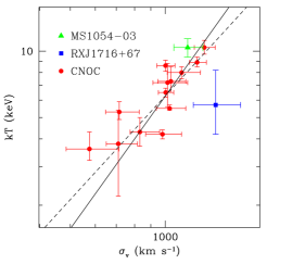
Figure 1.1: (Left) The relation between galaxy velocity dispersion, $\sigma_{v}$, and ICM temperature, $T$, for distant ($z>0.15$) galaxy clusters. Velocity dispersions are taken from Carlberg et al. (1997a)) for CNOC clusters and from Girardi & Mezzetti (2001)) for MS1054-03 and RXJ1716+67. Temperatures are taken from Lewis et al. (1999) for CNOC clusters, from Jeltema et al. (2001) or MS1054-03 and from Gioia et al. (1999) for RXJ1716+67. The solid line shows the relation $k_{B}T=\mu m_{p}\sigma_{v}^{2}$, and the dashed line is the best–fit to the low–$z$ $T$–$\sigma_{v}$ relation from Wu et al. (1999). (Right) The low-$z$ relation between X-ray luminosity and the mass contained within the radius encompassing an average density $200\rho_{c}$ (from Reiprich & Böhringer 2002). The two lines are the best log–log linear fit to two different data sets indicated with filled and open circles.

Observational data for nearby clusters (e.g. Wu et al. 1999) and for distant clusters (see Figure 1.1) roughly follow the above relation for the gas temperature. This correlation indicates that the assumption that clusters are relaxed structures in which both gas and galaxies feel the same dynamics is reasonable. Anyway, there are some exceptions that reveal the presence of a more complex dynamics.

At high energies, the ICM behaves as a fully ionised plasma, whose emissivity is dominated by thermal bremsstrahlung. The pure bremsstrahlung emissivity is a good approximation for $T\gtrsim 3$ keV clusters, but a further contribution from metal emission lines should be taken into account when considering cooler systems (e.g. Raymond & Smith 1977). By integrating the above equation over the energy range of the X-ray emission and over the gas distribution, one obtains X-ray luminosities $L_{X}\sim 10^{43}$-$10^{45}\,{\rm erg\,s^{-1}}$. These powerful luminosities allow clusters to be identified as extended sources out to large cosmological distances.

The condition of hydrostatic equilibrium connects the local gas pressure $p$ to its density $\rho_{\rm gas}$ according to

$${dp\over dR}\,=\,-{GM(<R)\rho_{\rm gas}(R)\over R^{2}}\,.$$ (1.42)

By substituting the equation of state for a perfect gas, $p=\rho_{\rm gas}k_{B}T/\mu m_{p}$ into the above equation, one can express the total gravitating mass within R as

$$M(<R)\,=\,-{k_{B}TR\over G\mu m_{p}}\,\left({d\,\log\rho_{\rm gas}\over d\log R}+{d\,\log T\over d\log R}\right)\,.$$ (1.43)

At redshift $z$, we have $M\propto R^{3}\bar{\rho}_{0}(1+z)^{3}\Delta_{vir}(z)$, where $R$ is the virial radius, $\bar{\rho}_{0}$ is the mean cosmic density at present time and $\Delta_{vir}(z)$ is the mean overdensity within a virialized region. For an Einstein–de-Sitter cosmology, $\Delta_{vir}$ is constant and therefore, for an isothermal gas distribution, Equation (1.43) implies $T\propto M^{2/3}(1+z)$. By measuring quantities such as $\rho_{\rm gas}$ and $T$ from X-ray observations, one can easily derive the mass of the selected cluster. Thus, in addition to providing an efficient method to detect clusters, X-ray studies of the ICM allow one to quantify the total gravitating cluster mass, which is the quantity predicted by theoretical models for cosmic structure formation.

A popular description of the gas density profile is the $\beta$–model,

$$\rho_{g}(r)\,=\,\rho_{g,0}\,\left[1+\left({r\over r_{c}}\right)^{2}\right]^{-3\beta/2},$$ (1.44)

which was introduced by Cavaliere & Fusco–Femiano (1976); see also Sarazin 1988, and references therein) to describe an isothermal gas in hydrostatic equilibrium within the potential well associated with a King dark-matter density profile. The parameter $\beta$ is the ratio between kinetic dark-matter energy and thermal gas energy. This model is a useful guideline for interpreting cluster emissivity, although over limited dynamical ranges. Now, with the Chandra and Newton-XMM satellites, the X-ray emissivity can be mapped with high angular resolution and over larger scales. These new data have shown that Equation 1.44 with a unique $\beta$ value cannot always describe the surface brightness profile of clusters (e.g. Allen et al. 2001).

Kaiser (1986) described the thermodynamics of the ICM by assuming it to be entirely determined by gravitational processes, such as adiabatic compression during the collapse and shocks due to supersonic accretion of the surrounding gas. As long as there are no preferred scales both in the cosmological framework (i.e. $\Omega_{m}=1$ and power–law shape for the power spectrum at the cluster scales), and in the physics (i.e. only gravity acting on the gas and pure bremsstrahlung emission), then clusters of different masses are just a scaled version of each other, because bremsstrahlung emissivity predicts $L_{X}\propto M\rho_{\rm gas}T^{1/2}$, $L_{X}\propto T_{X}^{2}(1+z)^{3/2}$ or, equivalently $L_{X}\propto M^{4/3}(1+z)^{7/2}$. Furthermore, if we define the gas entropy as $S=T/n^{2/3}$, where $n$ is the gas density assumed fully ionized, we obtain $S\propto T(1+z)^{-2}$.

It was soon recognized that X-ray clusters do not follow these scaling relations. The observed luminosity–temperature relation for clusters is $L_{X}\propto T^{\alpha}$, where $\alpha\sim 3$ for $T\gtrsim 2$ keV, and possibly even steeper for $T\lesssim 1$ keV groups. This result is consistent with the finding that $L_{X}\propto M^{\alpha}$ with $\alpha\simeq 1.8\pm 0.1$ for the observed mass–luminosity relation (e.g. Reiprich & Böhringer 2002; see right panel of Figure 1.1). Furthermore, the low-temperature systems are observed to have shallower central gas-density profiles than the hotter systems, which turns into an excess of entropy in low–$T$ systems with respect to the $S\propto T$ predicted scaling (e.g. Ponman et al. 1999, Lloyd–Davies et al. 2000).

1.3.2 Breaking of the scaling relations: the importance of non-gravitational heating

A possible interpretation for the breaking of the scaling relations assumes that the gas has been heated at some earlier epoch by feedback from a non-gravitational astrophysical source (Evrard & Henry 1991). This heating would increase the entropy of the ICM, place it on a higher adiabat, prevent it from reaching a high central density during the cluster gravitational collapse and, therefore, decrease the X-ray luminosity (e.g. Balogh et al. 1999, Tozzi & Norman 2001, and references therein). For a fixed amount of extra energy per gas particle, this effect is more prominent for poorer clusters, i.e. for those objects whose virial temperature is comparable with the extra–heating temperature. As a result, the self–similar behavior of the ICM is expected to be preserved in hot systems, whereas it is broken for colder systems. Both semi–analytical works (e.g. Cavaliere et al. 1998, Balogh et al. 1999, Wu et al. 2000; Tozzi et al. 2000) and numerical simulations (e.g. Navarro et al. 1995, Brighenti & Mathews 2001, Bialek et al. 2001 Borgani et al. 2001a) converge to indicate that $\sim 1$ keV per gas particle of extra energy is required. A visual illustration of the effect of pre–heating is reported in Figure 1.2, which shows the entropy map for a high–resolution simulation of a system with mass comparable to that of the Virgo cluster, for different heating schemes (Borgani et al. 2001b). The effect of extra energy injection is to decrease the gas density in central cluster regions and to erase the small gas clumps associated with accreting groups.

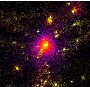
Figure 1.2: Map of gas entropy from hydrodynamical simulations of a galaxy cluster (from Borgani et al. 2001a). (Left): gravitational heating only. (Right): entropy floor of 50 keV/cm² imposed at $z=3$, corresponding to about 1 keV/part. Light colors correspond to low entropy particles, and dark blue corresponds to high–entropy gas.

The gas-temperature distributions in the outer regions of clusters are not affected by gas cooling. These temperature distributions have been studied with the ASCA and Beppo–SAX satellites. General agreement about the shape of the temperature profiles has still to be reached (e.g. Markevitch et al. 1998, White 2000, Irwin & Bregman 2000). De Grandi & Molendi (2002) analyzed a set of 21 clusters with Beppo–SAX data and found the gas to be isothermal out to $\sim 0.2R_{\rm vir}$, with a significant temperature decline at larger radii. Such results are not consistent with the temperature profiles obtained from cluster hydrodynamical simulations (e.g. Evrard et al. 1996, Borgani et al. 2003), thus indicating that some physical process is still lacking in current numerical descriptions of the ICM. Deep observations with Newton–XMM and Chandra will allow the determination of temperature profiles over the whole cluster virialized region.

Cooling in the Intra Cluster Medium

In order to characterize the role of cooling in the ICM, it is useful to define the cooling time–scale, which for an emission process characterized by a cooling function $\Lambda_{c}(T)$, is defined as $t_{cool}=k_{B}T/(n\Lambda(T))$, $n$ being the number density of gas particles. For a pure bremsstrahlung emission: $t_{cool}\simeq 8.5\times 10^{10}{\rm yr}\,(n/10^{-3}{\rm cm}^{-3})^{-1}\,(T/10^{8}K)^{1/2}\,.$ (e.g. Sarazin 1988). Therefore, the cooling time in central cluster regions can be shorter than the age of the Universe. A substantial fraction of gas undergoes cooling in these regions, and consequently drops out of the hot diffuse, X-ray emitting phase. Studies with the ROSAT and ASCA satellites indicate that the decrease of the ICM temperature in central regions has been recognized as a widespread feature among fairly relaxed clusters (see Fabian 1994, and references therein). The canonical picture of cooling flows predicted that, as the high–density gas in the cluster core cools down, the lack of pressure support causes external gas to flow in, thus creating a superpositions of many gas phases, each one characterized by a different temperature. Our understanding of the ICM cooling structure is now undergoing a revolution thanks to the much improved spatial and spectral resolution provided by Newton–XMM. Recent observations have shown the absence of metal lines associated with gas at temperature $\lesssim 3$ keV (e.g. Peterson et al. 2001, Tamura et al. 2001), in stark contrast with the standard cooling flow prediction for the presence of low–temperature gas (e.g. Böhringer et al. 2002a, Fabian et al. 2001a).

Radiative cooling has been also suggested as an alternative to extra heating to explain the lack of ICM self–similarity (e.g. Bryan 2000, Voit & Bryan 2002). When the recently shocked gas residing in external cluster regions leaves the hot phase and flows in, it increases the central entropy level of the remaining gas. In the meanwhile, gas “cools off” the hot phase: the decreased amount of hot gas in the central regions causes a suppression of the X-ray emission (Pearce et al. 2000, Muanwong et al. 2001). This solution has a number of problems. Cooling in itself is a runaway process, leading to a quite large fraction of gas leaving the hot diffuse phase inside clusters. Analytical arguments and numerical simulations have shown that this fraction can be as large as $\sim 50\%$, whereas observational data indicates that only $\lesssim 10\%$ of the cluster baryons are locked into stars (e.g. Bower et al. 2001, Balogh et al. 2001). This calls for the presence of a feedback mechanism, such as supernova explosions (e.g. Menci & Cavaliere 2000, Finoguenov et al. 2000, Pipino et al. 2002; Kravtsov & Yepes 2000) or Active Galactic Nuclei (e.g. Valageas & Silk 1999, Wu et al. 2000, Yamada & Fujita 2001), which, given reasonable efficiencies of coupling to the hot ICM, may be able to provide an adequate amount of extra energy to balance overcooling. We will summarize feedback mechanisms on Sec. 1.4.2 and  1.4.3.

1.3.3 The diffuse light in galaxy clusters

A significant stellar component of galaxy clusters is found outside of the galaxies. The standard theory of cluster evolution is one of hierarchical collapse, as time proceeds, clusters grow in mass through the merging with other clusters and groups. These mergers as well as interactions within groups and within clusters strip stars out of their progenitor galaxies.
In this section, we review the basic properties and observed characteristics of the optical diffuse light in clusters. In Chapter 3 we will show how studying this intracluster component in cosmological simulations of galaxy clusters can inform hierarchical formation models as well as tell us something about physical mechanisms involved in galaxy evolution within clusters.

The first reference in the literature about the diffuse light in cluster of galaxies was given by Zwicky (1951): “One of the most interesting discoveries made in the course of this investigation [in the Coma cluster] is the observation of an extended mass of luminous intergalactic matter of very low surface brightness. The objects which constitute this matter must be considered as the faintest individual members of the cluster. [We report] the discovery of luminous intergalactic matter concentrated generally and differentially around the center of the cluster and the brightest (most massive) galaxies, respectively”. This is a perfect characterization of the optical diffuse light in cluster: extended, low surface brightness and around the center of the cluster.

The characteristics of this diffuse stellar component published by Zwicky (1951, 1957, 1959) were qualitative: it has an extension of around 150 kpc, the color index is rather blue and produces a local absorption of light of the order of six tenth of a magnitude.

The first published attempt to obtain a value for the surface brightness $\mu$ of the faint intergalactic matter in Coma corresponds to de Vaucouleurs (1960). He reported an upper limit of $\mu$ $>$ 29.5 mag arcsec^-2. With this value, de Vaucouleurs reasons out that “a stellar population composed exclusively of extreme red dwarfs of mass M$<0.1$ M_⊙ and absolute magnitudes $M(pg)>+15$ would, in principle, give a mass-to-light ratio (M/L) ratio of the order measured in Coma. While such stars are known to exist in the neighborhood of the sun, it seems very difficult to admit that they could populate intergalactic space with the required density and to the exclusion of all other stars of slightly greater mass. Thus, de Vaucouleurs concludes that the mass of the intergalactic matter is not enough to account for the mass value estimated through the virial theorem.

Before the CCD detectors were widely used, most of the observations and study of the diffuse light in clusters was carried out in the Coma cluster (e.g. Abell (1965); Gunn (1969)) and in other rich clusters (e.g. the Virgo cluster: Holmberg (1958); de Vaucouleurs (1969)). The first accurate measurements of the diffuse light in Coma dated back to the beginnig of the nineties thanks to the introduction of the CCD photometry (Bernstein et al. 1995).

Observing the Intra Cluster Light (ICL) is quite problematic, first of all because it is expected to be extremely faint (about 25–26 mag arcsec^-2). Than, there a number of problems associated to the use of CCD’s, among them we review the following:

• ICL is expected to be extremely faint, thus detections are subjected to spurios effects, intrumental scattering and contamination due to bright stars or faint galaxies;

• if the cleanliness of the telescope optics is not correct enough, some of the results that we could ascribe to the intracluster light would be masked or spoiled;

The most important characteristics associated with the diffuse light in clusters of galaxies can be summarized as follows:

$\boldsymbol{Luminosity}$ It shows a wide range. The intracluster light can represent between the 10% and the 50% of the total light of the region where it is detected. Schombert (1988) finds some correlation, but faint, between the luminosity of the cD envelope and that of the underlying galaxy. This correlation can hint that the process of formation of the brightest cluster galaxy (BCG) has some reflection in the origin of its envelope.

$\boldsymbol{Color}$ Different authors have report various results. Valentijn (1983) in $B-V$ and Scheick & Kuhn (1994) in $V-R$ find blueward gradients that vary between 0.1 to 0.6 mag drop. Schombert (1988) in $B-V$ doesn’t find any evidence of strong color gradients or blue envelopes colors. Finally, Mackie (1992) in $g-r$ reports a reddening at the end of the envelopes, in one case of the order of 0.15 mag.

$\boldsymbol{Structure}$ Schombert (1988) and Mackie, Visvanathan & Carter (1990) find a apparent break in the surface brightness profile of the underlying cD galaxies. According to Schombert (1988), this break is found near the $24V$ mag arcsec^-2 but there are no sharp changes in either eccentricity or orientation between the galaxy and the envelope. However, Uson et al. (1991) and Scheick & Kuhn (1994) don’t see such a break in their studies. Reinforcing the idea of common evolutive processes, Schombert (1988) and Bernstein et al. (1995) find that the diffuse light, globular cluster density and galaxy density profiles seem to have similar radial structure.

Basically, there are three processes that could be responsible for the origin of the ICL. According to the first one, ICL originates from stars lying in the outer envelopes of galaxies. Sometimes the extension of the diffuse light is so large (several core radius) that is hard to believe that these stars are gravitationally bound to any galaxy, and probably, they are stripped material after the interaction between galaxies. This could be the case in Cl 1613+31 (Vílchez–Gómez et al. 1994a). Also, it could be that the stars have born directly in the intergalactic medium from a cooling flow, for example (Prestwich & Joy 1991).
According to the second process, ICL is given by dwarf galaxies and globular clusters. Part of the light in the intergalactic medium in distant clusters, where it is not possible to resolve dwarf galaxies and globular clusters, can have this origin. Nevertheless, Bernstein et al. (1995) have measure in the Coma cluster a diffuse light apart from dwarf galaxies and globular clusters.
Finally ICL can originate from light scattered by intergalactic dust. The existence of dust in rich clusters of galaxies as established by Zwicky (1959) or Hu (1992) would suggest the production of diffuse scattered light.

There are al least three theories that try to elucidate what is the origin and evolution of cD envelopes. None of them offers a complete picture of the problem.

Stripping theory

This theory was initially proposed by Gallagher & Ostriker (1972). According with this theory, the origin of the envelope is on the debris due to tidal interactions between the cluster galaxies. These stars and gas are then deposited in the potential well of the cluster where the BCG is located. This process begins after the cluster collapse and the envelope grows as the cluster evolves. The fact that different cD envelopes show different color gradients can be explained as the result of different tidal interaction histories: in some clusters the tidal interactions involve mainly spirals, but in others, early type galaxies are the source material (Schombert 1988). The main problem to this hypothesis is the difficulty to explain the observed smoothness of the envelopes as the timescale to dissolve the clumps is on the order of the crossing time of the cluster (Scheick & Kuhn 1994).

Primordial origin theory

This hypothesis, suggested by Merrit (1984), is similar to the previous one but, in this case, the process of removing stars from the halos of the galaxies was carried out by the mean cluster tidal field and took place during the initial collapse of the cluster. The BCG, due to its privileged position in relation with the potential well, gets the residuals that make up its envelope. However, this picture is difficult to reconciliate with the fact that there are cD’s with significant peculiar velocities (Gebhardt & Beers 1991) as well as with the smoothness of the diffuse light either the envelope is affixed to the cD or fixed and the cD is moving through it. Moreover, if the origin of the diffuse light is primordial, how can we explain the observation of blue color gradients in some envelopes, supposed little activity after virialization?

Mergers

Villumsen (1982, 1983) found that after a merger with the BCG, and under special conditions, it is possible to form an halo similar to that present in cD galaxies since there is a transfer of energy to the outer part of the mergers resulting an extended envelope. Although this theory reproduces the profile observed for the envelopes, it is not possible to accomplish for the luminosities and masses seen for the diffuse light. However, in poor clusters where there are cD-like galaxies without a clear envelope this mechanism can play a more important role (Thuan & Romanishin 1981; Schombert 1986).

1.4 Open questions in galaxy formation

After a decade of spectacular breakthroughs in physical cosmology, the focus has now been shifted away from determining cosmological parameters towards attacking the problem of galaxy formation. Consequently, the origin and evolution of galaxies are one of the current major outstanding questions of astrophysics.
Galaxy formation is driven by a complex set of physical processes with very different spatial scales. Radiative cooling, star formation and supernovae explosions act at scales less than 1 pc, but they affect the formation of the whole galaxy (Dekel & Silk, 1986). Active Galactic Nuclei act on galaxy scale and thus are thought to be play a fundamental role in regulating galaxy evolution. In addition, large–scale cosmological processes, such as gas accretion through cosmic filaments and galaxy mergers, control the general galaxy assembly.
Galaxies are, in their observable constituents, basically large bound systems of stars and gas whose components interact continually with each other by the exchange of matter and energy. The interactions that occur between the stars and the gas, most fundamentally the continuing formation of new stars from the gas, cause the properties of galaxies to evolve with time, and thus they determine many of the properties that galaxies are presently observed to have. Star formation cannot be understood simply in terms of the transformation of the gas into stars in some predetermined way, however, since star formation produces many feedback effects that control the properties of the interstellar medium, and that thereby regulate the star formation process itself. A full understanding of the evolution of galaxies therefore requires an understanding of these feedback effects and ultimately of the dynamics of the entire galactic ecosystem, including the many cycles of transfer of matter and energy that occur among the various components of the system and the magnetohydrodynamical (MHD) instabilities that regulate the cooling flow in hot galaxy clusters.
A comprehensive review on star formation and related topics (molecular clouds, triggering mechanisms, energy injection by SNe) will be given along chapters 2 and 3 by means of numerical models. In the following we first give some clues on the role that galactic magnetic field may have on the dynamics of galaxy formation and finally summarize the most accreditated form of energy feedback which are considered as an alternative to extra heating in explaining the lack of ICM self–similarity (see Sec. 1.3.2).

1.4.1 Galactic magnetic fields

Magnetic fields may significantly influence the structure and evolution of Inter Stellar Medium (ISM hereafter). This has been proven extensively by local magnetohydrodynamic (MHD) simulations of the ISM (Mac Low et al. 2005, Balsara et al.2004, de Avillez & Breitschwerdt 2005, Piontek & Ostriker 2007, Hennebelle & Inutsuka 2006) and by observations (e.g. Beck 2007, Crutcher 1999). On a larger scale, simulation are quite close to having the resolution necessary to properly describe the magnetic field components down to the observed scales. Cosmological MHD simulations have been done in SPH (e.g. Dolag 1999, 2002, 2005) in the context of galaxy cluster formation and in Eulerian-code simulations (e.g. Brüggen et al. 2005, Li et al. 2006).
The main open question in galactic MHD concerns the origin and the evolution of the magnetic field (MF) in galaxy clusters. Besides the variety of the possible contributors, the corresponding generated MF will be compressed and amplified by the process of structure formation. There are basically three main classes of models for the origin of cosmological MF:

• MF are produced “locally” at relatively low redshift ($z\sim$2–3) by galactic winds (e.g. Völk & Atoyan 2000) or Active Galactic Nuclei (e.g. Furlanetto & Loeb 2001);

• MF seeds are produced at higher redshifts, before galaxy clusters form gravitationally bound systems; the origin could still be starburst galaxies and AGN but at earlier times ($z\sim$ 4–5) ot seeds may have a comological origin;

• MF seeds are produced by the so–called Biermann battery effect (Kulsrud et al. 1997; Ryu, Kang & Biermann 1998). In few words, merger shocks generated during the hierarchical structure formation process give rize to small thermionic electric currents which in turn may generate MFs.

Supported by simulations of individual events/environments like shear flows, shock/bubble interactions or turbolence/merging events, all the above different models of seed MFs predict a super–adiabatic amplification of the MF. Anyhow, none of the present simulations include the creation of MF by all the feedback processes happening with the Large Scale Structure (e.g. radio bubbles, AGNs, galactic winds, etc.). Moreover, all the simulation done so far neglect radiative losses and thus the corresponding increase in density in the central parts of the clusters which would lead to a further MF amplification.
Following the dynamics of galaxies in cosmological simulation is a real challenge within LSS simulations. It is expected that once these limitations will be overcame, the dynamical impact of the MF on regions likes the cooling flows at the centre of galaxy clusters will be significant and will eventually contribute to solve important remarkable enigmas.

1.4.2 Active Galactic Nuclei feedback

Many galaxies reveal an active nucleus, a compact central region from which one observes substantial radiation that is not the light of stars or emission from the gas heated by them. Active Nuclei emit strongly over the whole electromagnetic spectrum, including the radio, X–ray, and $\gamma$–ray regions where most galaxies hardly radiate at all. The most powerful of them, the quasars, easily outshine their host galaxies. Many have luminosities exceeding $10^{12}$$L_{\odot}$ and are bright enough to be seen most of the way across the observable Universe.
In the standard model of AGN, cold material close to the central Black Hole (BH) forms an accretion disk. Dissipative processes during accretion transport matter inward and angular momentum outward, while causing the accretion disk to heat up. The radiation from the accretion disk excites cold atomic material close to the BH and this radiates via emission lines. At least some accretion disks produce jets, twin highly collimated and fast outflows that emerges form close to the disk.
The accretion process release huge amounts of energy to their surroundings, in various forms:

• in luminous AGN (Seyfert nuclei and quasars) the output is mostly radiative: this radiation can affect the environment through radiation pressure and radiative heating;

• in most accreting BH the kinetic energy output is as important as the radiative one, due to the presence of strong winds and jets.

In all cases, it is also present a significant output of energetic particles (“cosmic rays”, relativistic neutrons and neutrinos).
In the following we recapitulate the various forms of energy injection that we hinted above and their plausible effects on the gas surrounding an AGN:

Radiation Pressure

: exerts a force on the gas via electron scattering, scattering and absorption on dust, photoionisation or scattering in atomic resonance lines;

Radiative heating

: gas exposed to ionising radiation from AGN tends to undergo and abrupt transition from the typical CII region temperature $\sim 10^{4}$K, to a higher temperature and ionisation state when $P_{gas}$/$P_{rad}$ falls below some critical value. The main effect on the surrounding are mass evaporation from clouds, elimination of cool ISM phase, modification of ISM phase structure.

Kinetic energy

: when charged particles cross shock waves generated by jets in radio galaxies and by outflows in accreting BH, they are expected to lose considerable energy as they move out of the denser regions and of the radiation field. However, the exact mechanism of “cosmic rays” acceleration in Ages is still not known.

As we reviewed in this section, AGN feedback effects (enormous on the basis of energetic arguments) depend sensitively on both the form of feedback and the detailed structure of the environment. While the efficiency of feedback due to radiation is often small, the kinetic energy injected by Ages tends to be trapped inside the ambient medium, leading to a higher efficiency. For a deep description of AGN feedback mechanisms we address the reader to Begelman 2001.
Recent X-ray observations show that radio galaxies can blow long lasting “holes” in the ICM, and may offset the effects of radiative losses, providing a possible interpretation for the entropy “excess” with respect to the self-similar expectations and a possible source of heating for reproducing the break at the bright end of the luminosity function. As discussed in Sec. 1.3.2, it has been proposed that the entropy excess results from some universal external pre–heating process (AGN, population III stars, etc.) that occurred before most of the gas entered the dark halos. Alternatively, the hot gas in groups may be heated internally by Type II supernovae when the galactic stars form.

1.4.3 Type II Supernovae energy feedback

Stars more massive than about nine times the mass of the Sun become internally unstable and violently explodes as they end their lives, turning into a type II supernova or core-collapse supernova. By dying, they create and disperse their stardust, including the elements with masses near that of oxygen, and inject in the surrounding medium approximately $10^{51}$ erg. Therefore, the formation of massive stars leads to a number of negative feedback effects including ionisation, stellar winds, and supernovae explosion that reduce the efficiency of star formation by destroying star–forming clouds and dispersing their gas before most of it has been turned into stars. The physics behind these star formation related processes is in general poorly understood. Feedback processes arguably have the largest impact on the form of the theoretical predictions for galaxy properties, while at the same time being among the most difficult and controversial phenomena to model.
The initial motivation for invoking SNe feedback was to reduce the efficency of star formation in low mass haloes, in order to flatten the slope of the faint end of the predicted galaxy luminosity function and make it in line with observations (Cole 1991; White & Frenk 1991). In current simulations of hierarchical galaxy formation models, there are two main physical mechanisms that can transfer energy from SNe to the surrounding medium:

• Kinetic feedback: the energy released by the supernova is directly injected to surrounding gas via outwards velocity kicks. This causes cold gas to be ejected from the parent galaxy, mimicking the effect of a supernova driven wind (Larson 1974, Dekel & Silk). Ejection of cold gas out of star forming regions has been proven to be very efficient in lowering the star formation rate;

• Thermal feedback: the energy from the supernova heats the interstellar medium (katz 1992). This causes the ablation of cold clouds and a net reduction of the star formation efficiency.

In the following chapters we will study in detail the type II SNe feedback physics from the numerical point of view. The aim of the present PhD Thesis, in fact, is to investigate different numerical approaches and to introduce a new, physically-based sub grid model of star formation and SNII energy feedback.

Chapter 2 Numerical techniques for galaxy formation simulations

An important issue in theories of galaxy formation is the relative importance of purely gravitational processes (as N-Body effects, clustering, etc..) and of gas-dynamical effects involving dissipation and radiative cooling. White $\&$ Rees 1978.

Structure formation refers to a fundamental problem in physical Cosmology. When inhomogeneities in the matter field are still very small, we can describe the evolution of perturbations using simple linear differential equations. The complexity of physical behaviour of fluctuations in the non-linear regime makes it impossible to study the details exactly using analytical methods. For this reason, numerical simulations and semi–analytical models have became standard tools for studying galaxy formation.
A detailed understanding of galaxy formation in cold dark matter scenarios remains a primary goal of modern astrophysics. While the large scale range physics is sufficient to describe a number of observations, using almost solely gravitational forces, the scales relevant for galaxy formation requires many physical processes to be considered in addition to the already complex interaction of nonlinear gravitational evolution and dissipative gas dynamic. Observed cluster of galaxies are, in fact, composed by three distinct components, dark matter, diffuse gas and stars, which have a different physics behind. Codes following both DM and baryonic particles already exist but they still have short comings, mainly for two reasons: the lack of resolution and the complexity of the involved physics. In fact, if from one side we need to account for star formation physics, acting on small scales, from the other we need to consider large–scale cosmological processes, such as gas accretion through cosmic filaments and galaxy mergers, which instead control the general galaxy assembly. For example, the typical size of a cold gas cloud is about 10 – 100 pc, while that of a galaxy like the Milky Way is of order 20 kpc, and that of a galaxy cluster is of order 1 Mpc. Following in details the whole dynamical range is too computationally expensive, so usually one resort to simplified models of the complex hydrodynamical and astrophysical processes working at the interstellar medium scales (see Sec. 2.3).

2.1 N-body and SPH codes

Given the initial conditions (which depend on the adopted cosmological model), the purpose of any cosmological code is to follow the evolution of density fluctuations from the linear regime (up to $z\sim 50-100$) till the actual time ($z=0$). It is possible to represent part of the expanding Universe as a “box”containing a large number N of point masses interacting through their mutual gravity. To start a numerical simulation one has first to decide about the size of the box the evolution of which should be simulated. For a given number of particles (which is limited by the power of the computer) this is always a compromise between higher mass resolution (smaller boxes) and a representative volume of the Universe (larger box). The Universe is assumed to be homogeneous on scales larger than the box size by means of periodical boundary conditions.
Numerical N-body techniques offer a simple and effective tool for describing the dynamical evolution of self-gravitating systems and for investigating non-linear cosmological gravitational evolution. A number of numerical techniques are available at the present time; they differ, for the most part, only in the way the forces on each particle are computed. Whereas N-body simulations are applied to a wide range of different astrophysical problems, the most appropriate technique to use depends on the specific context. In the following we briefly describe some of the most popular methods. For a comprehensive review on simulation techniques for cosmological simulations see e.g Dolag et al. 2008.

Direct sum (Particle-Particle, PP)

the gravitational interaction is computed by summing directly the (pairwise) contributions of all the individual particles to calculate the Newtonian forces. Despite its accuracy, direct summation requires a prohibitive computational cost (i.e. computing time $t$ scales as $N^{2}$) and is thus of difficult application in large scale numerical simulations.

Particle-Mesh (PM) methods

are the fastest scheme for computing the gravitational field. The forces are solved by assigning mass points to a regular grid and then solving Poisson’s equation on it in the Fourier space The use of a regular grid naturally provide periodic boundary conditions and allows one to use Fast Fourier Transform (FFT) methods to recover the potential, which leads to a considerable increase in speed ($t\sim N_{g}\log N_{g}$, where $N_{g}$ is the number of grid points). This method is well suited for cosmological simulations since allows the use of a large number of particles but the force resolution is given by the finite spatial size of the mesh which can’t be infinitely large. A substantial increase in spatial resolution can be achieved by using a hybrid “particle-particle-particle-mesh” method, which solves the the short range forces by direct summation (PP) but uses the mesh to compute those of longer range (PM). This scheme is usually called $P^{3}M$ ($PP+PM$) and achieves a good compromise between computational cost and accuracy of the solutions coming from PP and PM methods. In high density regions, however, the PP method dominates, degrading the code performance. If this is the case, the adaptive $P^{3}M$ method defines a number of sub-grids over which the PM computation is repeated, thus limiting the use of PP summation.

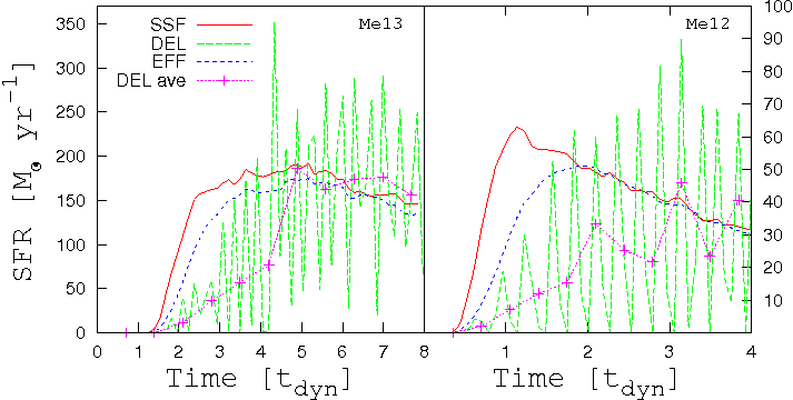
Figure 2.1: Schematic illustration of the Barnes & Hut (1986) oct-tree in two dimensions. The particles are first enclosed in a square (root node). This square is then iteratively subdivided into four squares of half the size, until exactly one particle is left in each final square (leaves of the tree). In the resulting tree structure, each square can be the progenitor of up to four siblings. Taken from Springel et al. 2001.

Tree codes

the computational domain is recursively partitioned into a hierarchy of cells containing one or more particles. Every cell which contains more than one particle is divided into $2^{3}$ sub-cells. If any of the resulting sub-cells contains more than one particle, that cell is subdivided again (see Fig. 2.1). The essence of a tree code is the recognition that the gravitational potential of a distant group of particles can be well-approximated by a low-order multipole expansion. In a tree code, a set of particles is arranged thus in a hierarchical system of groups that form of a tree structure. Thus, when the force on a particular particle is computed, the force exerted by distant particles is treated using the coarsely grained distribution contained in the higher level of the tree, the force being consequently approximated by their lowest multipole moments. In this way, the computational cost for a complete force evaluation can be reduced to ${\cal O}(N\log N)$ (Appel, 1985). In Sec. 2.2.1, we will study in detail the tree algorithm implemented in the GADGET-2 code Springel 2005. The greatest problem with such codes is that, although they run quite quickly in comparison with particle-mesh methods with the same resolution, they do require considerable memory resources. Moreover implementing periodic boundary conditions is much more difficult than in PM codes. Periodic boundary conditions for tree codes are usually obtained by a numerical technique called “Ewald summation” (Ewald, 1921).

Following the non-linear gravitational evolution of collisionless dark matter however is not enough if one aims to obtaining precise informations on the distribution of luminous matter. In this case, collisionless dynamics must be coupled to gas dynamics.
The fundamental equations regulating the evolution of a collisional fluid (gas) are, in comoving coordinates:

$$\frac{\partial}{\partial t}(\frac{\rho_{b}}{\bar{\rho_{b}}})+\frac{1}{a}\boldsymbol{\nabla}\cdot\boldsymbol{v_{b}}=0$$ (2.1)

$$\frac{\partial\boldsymbol{v_{b}}}{\partial t}+\frac{1}{a}\boldsymbol{v_{b}}\cdot\boldsymbol{\nabla}\boldsymbol{v_{b}}+H\boldsymbol{v_{b}}=-\frac{1}{a\rho_{b}}\boldsymbol{\nabla}p+\boldsymbol{g}$$ (2.2)

where $\rho_{b}$ is the density of baryons, $\bar{\rho_{b}}$ is the average density of baryons, $\boldsymbol{v_{b}}$ is the peculiar velocity, $p$ the pressure, $a$ the scale factor e $\boldsymbol{g}$ the gravitational field.
An equation for energy or entropy has to be added to the above equations. Outside shocks, the equations for thermal energy and entropy evolution can be written respectively as:

$$\frac{\partial U}{\partial t}+\frac{1}{a}\boldsymbol{v_{b}}\cdot\boldsymbol{\nabla}U=\frac{p}{a\rho_{b}}\boldsymbol{\nabla}\cdot\boldsymbol{v_{b}}+\frac{1}{\rho_{b}}(\Gamma-\Lambda)$$ (2.3)

$$\frac{\partial S}{\partial t}+\frac{1}{a}\boldsymbol{v_{b}}\cdot\boldsymbol{\nabla}S=\frac{1}{p}(\Gamma-\Lambda)$$ (2.4)

where $\Gamma$ and $\Lambda$ are respectively the heating and the cooling rates.
For a perfect gas with specific heat $c_{v}$

$$U=\frac{p}{[(c_{v}-1)\rho_{b}]}\qquad\textrm{thermal energy per unit mass}$$ (2.5)

$$S=(c_{v}-1)^{-1}ln(p\rho_{b}^{-c_{v}})\qquad\textrm{entropy per unit mass}$$ (2.6)

To close the system, an equation of state relating the thermodynamical variables needs to be specified. This is:

$$P=(\gamma-1)\rho U$$ (2.7)

where $\gamma=\frac{5}{3}$ is the adiabatic exponent for a monoatomic ideal gas.
Due to the non-linear nature of the equations of hydrodynamics, exact solutions of these equations are rarely found.
There are two principle algorithms in common use to follow the hydrodynamics of gas in an expanding universe: particle based, Lagrangian schemes, which employ a technique called smoothed particle hydrodynamics (SPH, Lucy, Gingol & Monaghan 1977, Monaghan 1992; Couchman, Thomas & Pearce 1995; Gnedin 1995; Springel & Hernquist 2003; Wadsley, Stadel & Quinn 2004) and grid based, Eulerian schemes (e.g. Ryu et al. 1993; Cen & Ostriker 1999). We here focus on Lagrangian scheme, for a description of grid-based methods see e.g. Dolag et al. 2008.
In smoothed particle hydrodynamics (SPH) one typically represents the fluid as a set of particles in the same way as in the N-body gravitational case, described before in this section. SPH is thus an extension of N-body techniques, making simple its integration in pre-existing cosmological codes.
The basic idea characterising SPH is to discretise the fluid by mass elements: fluid variables, such as baryonic density, temperature and velocity, are evolved using particle with constant mass. Since SPH is a Lagrangian method, equation 2.1 (the mass continuity equation) can be neglected. The thermodynamics variables $q$ are estimated by a smoothing kernel $W$ from which we obtain:

$$q(\boldsymbol{x})=\sum_{i=1}^{N}q_{i}W(\boldsymbol{x}-\boldsymbol{x}_{i},h)$$ (2.8)

where $q_{i}$ is the studied quantity and ${\vec{x}_{i}}$ its position while $h$ is the smoothing length. This method consists in assuming that the quantities are “smoothed” into a region of finite dimension, centred on each particle, rather than being punctiform. The summation  2.8 extends only over particles lying within a cutoff radius proportional to $h$. Usually $h$ is taken to be proportional to $\rho_{b}^{-1/3}$: in this way, we are sure to include in the above summation at least $N_{SPH}$= 30-40 particles. In this case, the number of particles inside smoothing radius $h$ is nearly equal to $N_{SPH}$. Alternatively, adaptive smoothing lengths $h_{i}$ of each particle are defined such that their kernel volumes contain a constant mass for the estimated density, i.e. smoothing lengths and densities obey the equation:

$$\frac{4\pi}{3}h_{i}^{3}\rho_{i}=N_{\small SPH}\bar{m}$$ (2.9)

where $N_{\small SPH}$ is the typical number of smoothing neighbours and $\bar{m}$ is an average particle mass.
SPH has some special advantages over the traditional grid-based methods, the most important among which is its adaptive Lagrangian nature: SPH follows the motion of the fluid and thus is not affected by the arbitrariness of the particle distribution. In practical terms, this means that most of the computing effort is directed towards places where most of the particles are. An important disadvantage of SPH is that it has to rely on an artificial viscosity for supplying the necessary entropy injections in shocks (see Sec. 2.2.2). On the contrary, Mesh-codes offer superior resolving power for hydrodynamical shocks. However, static meshes are only poorly suited for the high dynamic range encountered in cosmology.

2.2 GADGET-2

GADGET (GAlaxies with Dark matter and Gas intEracT, Springel et al. 2001) is a freely available, parallel code which uses the standardised MPI communication interface.
GADGET computes gravitational forces with a hierarchical tree algorithm (optionally in combination with a particle-mesh scheme for long-range gravitational forces) and represents fluids by means of smoothed particle hydrodynamics (SPH). The code can be used both for studies of isolated self-gravitating systems, and for cosmological simulations. Both the force computation and the time stepping of GADGET are fully adaptive.
A complete review of its features is given in a number of articles by its author, Volker Springel, so we will refer to them for all the details about the code. In the following, we will give a brief summary of the physics implemented in GADGET.

2.2.1 Collisionless dynamics

In an expanding background Universe, DM and stars are commonly treated as collisionless fluids and are described by the collisionless Boltzmann (or Vlasov) equation (CBE), which in comoving coordinates becomes:

$$\frac{\partial f}{\partial t}+\frac{{\vec{p}}}{ma^{2}}{\vec{\nabla}}f-m{\vec{\nabla}}\Phi\frac{\partial f}{\partial{\vec{p}}}=0\qquad\qquad\textrm{CBE}$$ (2.10)

where $a$ is the scale factor describing the spatial extent of the Universe, $f({\vec{x}},{\vec{p}},t)$ is the phase–space distribution function of the fluid and ${\vec{\nabla}}\Phi$ is the solution to the Poisson equation (Eq. 1.15). The fluid is thus represented in the phase space by a finite number N of tracer particles which are integrated along the characteristic curves of the CBE.
The gravitational attraction between particles is expressed in terms of the Newton’s equations of motion. In order to suppress large-angle scattering in two-body collisions, GADGET introduces a softening into the gravitational potential at small separations, which effectively introduces a lower spatial resolution cut-off.
As we mentioned before, the gravitational force is described by a tree code (see Sec. 2.1), where particles are arranged in a hierarchy of groups. The authors employed the Barnes and Hut (BH,1986) tree construction: the computational domain is hierarchically partitioned into a sequence of cubes, where each cube contains eight siblings, each with half the side-length of the parent cube. The tree is constructed such that each node (cube) contains one particle or is the progenitor to further nodes (see Fig. 2.1), in which case the node carries the monopole and quadrupole moments of all the particles that lie inside the cube.
The force computation then proceeds by “walking” the tree and summing up the appropriate force contributions form tree nodes. In the standard BH tree walk, the multipole expansion of a node of size $l$ is carried out if the distance $r$ of the point of reference to the centre-of-mass of the cell satisfies:

$$r>\frac{l}{\theta}\,,$$ (2.11)

where $\theta$ is an accuracy parameter which plays the role of a angle of view. If a node fulfils the criterion (2.11), the tree walk along this branch can be terminated, otherwise it is ‘opened’, and the walk is continued with all its siblings. For smaller values of the opening angle, the forces will in general become more accurate, but also more costly to compute. The geometric criterion  2.11 can therefore cause high errors in the force computation and does not guarantee a sufficient accuracy, so that other conditions must be fulfilled. We leave a complete discussion to Springel 2001, 2005.

2.2.2 Hydrodynamics

The gas, defined as perfect and non-viscous, is described by the SPH method.
The computation of the hydrodynamic force and the rate of change of internal energy proceeds in two phases. In the first phase, new smoothing lengths $h_{i}$ are determined for the active particles (these are the ones that need a force update at the current time-step), and for each of them, the neighbouring particles $j$ inside their respective smoothing radii are found. The Lagrangian nature of SPH arises when this number of neighbours is kept either exactly, or at least roughly, constant. This is achieved by varying the smoothing length $h_{i}$ of each particle accordingly.
Having found the neighbours, the SPH density is estimated as

$$\rho_{i}=\sum_{j=1}^{N}m_{j}W_{ij}(|r_{i}-r_{j}|,h_{i})$$ (2.12)

where $W_{ij}$ is the SPH smoothing kernel (see below).
In the second phase, the actual forces are computed.

Entropic formulation of SPH

In the conventional implementation of SPH (Monaghan 1992), the hydrodynamical equations are implemented using the thermal energy as an independent variable: while total energy is manifestly conserved, the same is not true for the entropy. Moreover the thermal energy version of SPH leads to substantial overcooling in halos that are resolved with up to a few thousand particles. Under low resolution conditions, the cooling rates of the gas are substantially overestimated, behaviour that may in part explain why cosmological SPH simulations predict more gas cooling than is expected based on simple analytic models (Pearce et al. 2001; Benson et al. 2001). Moreover, in hierarchical scenarios of structure formation, larger systems will inherit this problem if their progenitors suffered from overcooling. A further problem of the standard implementation of SPH is that point-like energy injection in the ISM, as those due to SNe feedback, can lead to unphysical negative temperatures. Hernquist (1993) has shown that, using the “energy” implementation of SPH, it is not possible to conserve simultaneously energy and entropy.
GADGET employs a new formulation of SPH which conserves energy and entropy (when appropriate) by construction, in which the dynamical equations are given as a function of entropy (Springel & Herquist, 2002). In this new implementation, the equations describing the evolution of a fluid are expressed as:

Discretisation of the equation for entropy evolution

$$\frac{dA_{i}}{dt}=-\frac{\gamma-1}{\rho_{i}^{\gamma}}L(\rho_{i},u_{i})+\frac{1}{2}\frac{\gamma-1}{\rho_{i}^{\gamma-1}}\sum_{j=1}^{N}m_{j}\Pi_{ij}\boldsymbol{v_{ij}}\nabla_{i}\bar{W_{ij}}$$ (2.13)

where $A(s)=u\frac{\gamma-1}{\rho^{\gamma-1}}$ is the entropic function, $\gamma$ is the adiabatic index, $L(\rho_{i},u_{i})$ is the emissivity per unit volume (introduced to describe external sinks or sources of energy due to radiative cooling or heating), $\Pi_{ij}$ denotes the artificial viscosity, $W_{ij}$ is the smoothing kernel (see below) and $v_{ij}$ is the relative velocity between fluid elements $i$ and $j$. The artificial viscosity term (Steinmetz, 1996) is introduced to take into account numerical effects due to gas shocks.

Equation of motion

$$\frac{d\boldsymbol{v_{i}}}{dt}=-\sum_{j=1}^{N}m_{j}[f_{i}\frac{P_{i}}{\rho_{i}^{2}}\nabla_{i}W_{ij}(h_{i})+f_{i}\frac{P_{j}}{\rho_{j}^{2}}\nabla_{i}W_{ij}(h_{j})]$$ (2.14)

where the $f_{i}$ are defined by:

$$f_{i}=(1+\frac{h_{i}}{3\rho_{i}}\frac{\partial\rho_{i}}{\partial h_{i}})$$ (2.15)

As mentioned before, an artificial viscosity term is incorporated for handling of shocks. The evolution of the corresponding “artificial” viscous force is given by:

$$\frac{d\boldsymbol{v_{i}}}{dt}\mid_{visc.}=-\sum_{j=1}^{N}m_{j}\Pi_{ij}\nabla_{i}\bar{W_{ij}}$$ (2.16)

This term added to acceleration  2.14, allows to completely describe the shocks. The resulting dissipation of kinetic energy is exactly balanced by a corresponding increase in thermal energy if the entropy is evolved according to equation (2.13).

The smoothing kernel used in GADGET is of the form:

$$W(r,h)=\frac{8}{\pi h^{3}}\left\{\begin{array}[]{ll}1-6(\frac{r}{h})^{2}+6(\frac{r}{h})^{3},&0\leqslant\frac{r}{h}\leqslant\frac{1}{2}\\ 2(1-\frac{r}{h})^{3},&\frac{1}{2}<\frac{r}{h}\leqslant 1,\\ 0,&\frac{r}{h}>1.\end{array}\right.$$ (2.17)

The entropic formulation of SPH solves satisfactorily (but not completely) some problems of the standard implementation. It provides one of best technique for modelling the process of point-like energy injection, which is relevant for certain feedback algorithms. It also reduces artificial overcooling in poorly resolved halos by a factor of $\sim$ 2 with respect to the standard implementation.
A more complete physical treatment of radiative heating/cooling and of energy feedback in GADGET is given in the following section.

2.2.3 Cooling and star formation

A proper modelling of the formation and evolution of the luminous component of galaxies is known to be an hard task. In order to properly describe the large number of physical processes involved in the interstellar medium (ISM) dynamics, we need to couple the already complex interaction of non-linear gravitational evolution and dissipative gas dynamics to a treatment for radiative heating and cooling and for the coagulation and fragmentation of molecular cold clouds.

Radiative cooling

On the contrary with dark matter, gas can cool via a number of mechanisms (see, for example, the discussion in Kauffmann & White 1994). The relative importance of the various mechanisms depends upon the conditions in the universe at the time the gas is cooling and the temperature of the gas. The principal cooling channels are: (i) Inverse Compton scattering of CMB photons by electrons in the hot halo gas (independent from density and temperature); (ii)Bremsstrahlung radiation as electrons are accelerated in an ionised plasma; (iii) decay/excitation of rotational or vibrational energy levels in molecular hydrogen through collisions.
Gas undergoing radiative cooling plays a key role in the process of star formation, since it rules the collapse of gas in the dark matter potential wells.
In GADGET, the equation regulating the energy loss per unit mass due to radiative cooling is given by:

$$(\frac{du}{dt})_{cool}=-\frac{\Lambda_{net}(\rho,T)}{\rho}$$ (2.18)

The authors have computed the cooling function $\Lambda_{net}(\rho,T)$ from the radiative processes appropriate for a primordial plasma of hydrogen and helium, neglecting variations in the metalicity of the gas as described in Katz et al. (1996). The suffix “net” denotes that the cooling function accounts for the presence of an external UV background field, which the authors take to be a modified Haardt & Madau (1996) spectrum. In high density regions, where radiative cooling is strong, the cooling times can become shorter than the dynamical free-fall timescale. In this case, the gas cools so quickly that dynamical processes are unable to adjust the pressure distribution: pressure support is lost and the gas undergoes a rapid collapse, causing the so-called “cooling catastrophe” and the subsequent formation of cold dense knots of gas.

White & Rees (1978) proposed a solution to this problem: energy released from stars in the course of their evolution would act as a negative feedback on the gas, thus limiting its cooling rate and associated star formation.
In the ISM, the gas exists in a wide range of density and temperature states (e.g. McKee & Ostriker 1977) and may thus be considered as a multiphase system resulting from the interplay of processes such as gravity, hydrodynamics, star formation, shocking by SNe and stellar winds, magnetic fields , cosmic rays, chemical enrichment and dust formation (Field 1965; Ferrara et al. 1995; Efstathiou 2000). Each process introduces its own length and time scales which often differs by orders of magnitude form those of the galaxy as a whole. As a result, a realistic description of the galactic environment is one of the most outstanding challenges in modern theoretical physics.

Effective hybrid multiphase Star Formation model

Springel & Hernquist (2003, SH03) named their treatment of star formation and feedback a “hybrid” method because it does not attempt to explicity resolve the spatial multiphase structure of the ISM on small scales, but rather makes the assumption that important aspects of the global dynamical behaviour of the ISM can be characterised by an effective “sub-resolution” model that uses only spatially averaged properties to describe the medium. The ISM is depicted as a fluid containing condensed cold clouds in pressure equilibrium with an ambient hot gas. The basic processes driving mass exchanges between the hot and the cold phase are: star formation, cloud evaporation due to SNe, cloud growth due to cooling and finally processes leading to the development of galactic winds.

There are two variants of the SH03 multi-phase model: one “explicit” where the treatment of mass and energy exchange among the different gas phases is followed explicitly and one “effective”, where the ISM sub-grid properties are derived each time-step from equilibrium solutions of equations describing the self-regulated SF. In the following we describe the effective SH03 model, being the one used in this PhD work. Within the effective star formation model, SH03 assumes that conditions for self-regulated star formation always hold without following the response of the star formation and feedback physics to variations of the thermodynamics state of the gas particle from one timestep to the following. The star forming particle thus passes from an equilibrium solution to the next one in a very short time, given by an external decay time parameter. The model provides the mass fraction in cold clouds x = ${\rho_{c}}/{\rho}$ and the density threshold $\rho_{\rm thr}$ for the onset of star formation. A detailed account of the star formation algorithm is presented in SH03, below we summarise the main features of the model. In the following description, $\rho_{h}$ denotes the local density of the hot ambient gas, $\rho_{c}$ is the density of cold clouds, $\rho_{\star}$ the density of stars, and $\rho=\rho_{h}+\rho_{c}$ is the total gas density. The average thermal energy per unit volume of the gas is then written as $\epsilon=\rho_{h}u_{h}+\rho_{c}u_{c}$, where $u_{h}$ and $u_{c}$ are the energy per unit mass of the hot and cold components, respectively.

The density threshold is fixed by requiring that the specific internal energy of a gas particle having a temperature of $10^{4}$ K is equal to the effective specific internal energy given by the model. In our runs, this corresponds to a gas numerical density $n_{\rm thr}\sim 0.25$ cm^-3. Once a gas particle density is above the star formation threshold it becomes eligible to form stars. In this PhD thesis work, we used the values suggested by SH03 for all parameters.

Star formation converts cold clouds into stars on a characteristic timescale $t_{\star}$. A mass fraction $\beta$=0.1 of these stars are short-lived and instantly die as SNe. Calling $\rho_{c}$ the average density of the cold gas, this process is described by the equation:

$$\frac{d\rho_{\star}}{dt}=(1-\beta)\frac{\rho_{c}}{t_{\star}}\qquad\qquad\textrm{\small{STAR FORMATION}}$$ (2.19)

The star formation rate (SFR) of a gas particle of mass m is given by:

$$\dot{M_{\star}}=(1-\beta)x\frac{m}{t_{\star}}$$ (2.20)

$x$ being the fraction of gas in cold clouds.

In addition to returning gas to the hot phase of the ISM, SNe also release energy $\epsilon_{\rm SN}$. Given the adopted Salpeter IMF, EFF expects an average return of energy per unit mass in formed stars of $\epsilon_{\rm SN}=4\cdot 10^{48}$ erg $M_{\odot}^{-1}$. This energy is injected into the hot phase, whose density and internal energy are $\rho_{h}$ and $u_{h}$. The heating rate due to SNe is then:

$$\frac{d}{dt}(\rho_{h}u_{h})\mid_{\rm SN}=\beta u_{\rm SN}\frac{\rho_{c}}{t_{\star}}\qquad\qquad\textrm{\small{SNe ENERGY FEEDBACK}}$$ (2.21)

where $u_{\rm SN}\equiv(1-\beta)\beta^{-1}\epsilon_{\rm SN}$ is the specific energy released by one SN.

Exploding supernovae, besides directly heating the ambient hot phase, evaporate the cold clouds residing inside the supernova-generated bubbles , essentially by thermal conduction. This can be described by:

$$\frac{d\rho_{c}}{dt}\mid_{EV}=A\beta\frac{\rho_{c}}{t_{*}}\qquad\qquad\textrm{\small{EVAPORATION}}$$ (2.22)

The efficiency $A$ of the evaporation process is expected to be a function of the local environment. In this work, $A$ is et to 1000.
The process by which cold clouds come into existence and grow is driven by radiative cooling (described above in this section). SH03 assume that a thermal instability operates in the region of coexistence between the cold and the hot phases, leading to mass exchanges among them. This mass flux is described by:

$$\frac{d\rho_{c}}{dt}\mid_{TI}=-\frac{\rho_{h}}{dt}\mid_{TI}=\frac{1}{u_{h}-u_{c}}\Lambda_{net}(\rho_{h},u_{h})\qquad\textrm{\small{CLOUD GROWTH due to COOLING}}$$ (2.23)

Temperatures of and total volumes occupied by the hot and cold phases are assumed to remain constant during cloud growth.

Quantitatively, the evolving rates of hot and cold masses can be written as:

$$\frac{d\rho_{c}}{dt}=-\frac{\rho_{c}}{t_{*}}-A\beta\frac{\rho_{c}}{t_{*}}+\frac{1-f}{u_{h}-u_{c}}\Lambda_{net}(\rho_{h},u_{h})$$ (2.24)

$$\frac{d\rho_{h}}{dt}=\beta\frac{\rho_{c}}{t_{*}}+A\beta\frac{\rho_{c}}{t_{*}}-\frac{1-f}{u_{h}-u_{c}}\Lambda_{net}(\rho_{h},u_{h})$$ (2.25)

The energy budget of the gas is thus given by:

$$\frac{d}{dt}(\rho_{h}u_{h}+\rho_{c}u_{c})=-\Lambda_{net}(\rho_{h},u_{h})+\beta\frac{\rho_{c}}{t_{*}}u_{SN}-(1-\beta)\frac{\rho_{c}}{t_{*}}u_{c}$$ (2.26)

where $u_{SN}=(1-\beta)/\beta\epsilon_{SN}$, otherwise defined as a “supernova temperature” $T_{\rm SN}=2\mu u_{\rm SN}/(3K)\sim 10^{8}{\rm K}$.
The above equation can be splitted into two separate relations for the energy of the hot and cold phase:

$$\frac{d}{dt}(\rho_{c}u_{c})=-\frac{\rho_{c}}{t_{*}}u_{c}-A\beta\frac{\rho_{c}}{t_{*}}u_{c}+\frac{(1-f)u_{c}}{u_{h}-u_{c}}\Lambda_{net}$$ (2.27)

$$\frac{d}{dt}(\rho_{h}u_{h})=\beta\frac{\rho_{c}}{t_{*}}(u_{SN}+u_{c})+A\beta\frac{\rho_{c}}{t_{*}}u_{c}-\frac{u_{h}-fu_{c}}{u_{h}-u_{c}}\Lambda_{net}$$ (2.28)

The equation for the energy of the hot phase after some calculus becomes:

$$\rho_{h}\frac{d}{dt}(u_{h})=\beta\frac{\rho_{c}}{t_{*}}(u_{SN}+u_{c}-u_{h})-A\beta\frac{\rho_{c}}{t_{*}}(u_{h}-u_{c})-f\Lambda_{net}$$ (2.29)

which gives the evolving equation for the temperature of the hot phase. It is easy to show from the previous equation that the internal energy of the hot phase is set by:

$$u_{h}=\frac{u_{\rm SN}}{1+A}+u_{c}$$ (2.30)

where $u_{c}=2\cdot 10^{44}$ erg $M_{\odot}^{-1}$ is the internal energy of the cold phase (assumed to be at 1000 K) and $A=(\rho/\rho_{\rm thr})^{-0.8}\cdot\beta$ is the efficiency of evaporation. Deviations from this temperature decay on a timescale $\tau_{h}=t_{\star}\rho_{h}/(\beta(A+1)\rho_{c})$, therefore, provided SF is rapid compared to adiabatic heating and radiative cooling, the temperature of the hot phase will be maintained at the value set by Eq. 2.30, independent of $t_{\star}$ and on the thermodynamics of the gas as given by its SPH evolution.
A further interesting features of SH03 model is that it leads to a self-regulated cycle of SF, where the growth of clouds is balanced by their evaporation owing to SNe feedback.

In order to help simplify the model, in the effective version of the SH03 model, the build-up of the stellar component is not described ‘smoothly’, as in the explicit one, but probabilistically. Given a time-step $\Delta t$, a new star particle of mass $m_{\star}$ = $m_{0}/N_{G}$ is spawned once a random number drawn uniformly from the interval [0,1] falls below:

$$p_{\star}=\frac{m}{m_{\star}}\bigg{\{}1-exp\bigg{[}-\frac{(1-\beta)x\delta T}{t_{\star}}\bigg{]}\bigg{\}}$$ (2.31)

Here $m_{0}$ is the initial gas mass of the SPH particle and $N_{G}$ (set to $N_{G}$=4 in our runs) gives the number of “generations” of stars that each particle may form. Each star particle always gets a mass $m_{0}/N_{G}$. This approach is quite mandatory to avoid both an uncontrolled multiplication of the number of particles and an artificial dynamical coupling of the gas with the stars.

Galactic winds

Galactic winds and outflows may be a fundamental mechanism in regulating star formation on galactic scales (Scannapieco, Ferrara & Broadhurst 2000). In fact, winds can reheat and trasport collapsed material from the center of a galaxy back to its extended dark matter halo and therefore can help to reduce the overall cosmic star formation rate to a level consistent with observational constraints. Moreover, galactic winds may help in solving the “overcooling” problem, provided that they can expel sufficient quantities of gas from low-mass galaxies. For these reasons, the SH03 model has been extended to account for galactic winds driven by star formation.
The wind model can be summarized as follows. First, the disk mass-loss rate that goes into wind, $\dot{M}_{w}$ is proportional to the star formation rate itself $\dot{M}_{\rm w}=\eta\dot{M}_{\star}$, where $\eta$ is the wind efficiency. This assumption is based on observational evidences (Martin 1999) and tells nothing about the ability of this gas to escape from the potential well. Second, it is assumed that the wind carries a fixed fraction $\chi$ of the supernova energy. The wind velocity is thus obtained by equating the kinetic energy in the wind with the energy input by supernovae,

$$\frac{1}{2}\dot{M_{w}}v_{w}^{2}=\chi\epsilon_{SN}\dot{M_{*}}$$ (2.32)

and it is equal to:

$$v_{w}=\sqrt{\frac{2\beta\chi u_{SN}}{\eta(1-\beta)}}$$ (2.33)

All the star forming gas particles can enter the wind if chosen by the probabilistic criterion given by Eq. 2.31. The net effect of the wind is to remove cold gas from the potential well, thus halting star formation.
When wind particles depart from the inner parts of the star-forming regions, their kinetic energy is thermalized inside the region itself due to hydrodynamical interactions. To let the wind particles to freely escape from star-forming dense regions, a “decoupling” mechanism of the wind particles from the hydrodynamical interactions is provided (see Sec. 2.3.2 for the Della Vecchia & Schaye 2008 “coupled” wind model).

2.3 Modelling star formation and SNe energy feedback

Including astrophysical processes in simulations such as radiative cooling of the gas, star formation and energy feedback from SuperNovae (SNe) (see Dolag et al. 2008), is a hard task for several reasons. The physics of star formation is complex and currently not understood in full detail. Moreover, the ISM besides being multi-phase is also multi-scale; the dynamical range needed to simultaneously resolve the formation of cosmic structures and the formation of stars is huge, since the former process happens on Mpc scales at densities of 10^-7 atoms ${\rm cm^{-3}}$ and the latter on parsec scales at typical densities greater than 100 atoms ${\rm cm^{-3}}$. This calls for resolving seven orders of magnitude in length scale, and about ten orders of magnitude in density. This can only get worse if we aim at following directly the process of star formation. As a consequence, numerical simulations commonly use simple “sub-grid” prescriptions (Yepes et al. 1997, SH03, Marri & White 2003, Scannapieco et al. 2006, Booth et al. 2006) for example to reduce the required dynamical range and account for star formation and SN energy feedback, thus hiding the complexity of the star formation process. Early attempts to introduce stellar feedback into simulations (Baron & White 1987, Cen & Ostriker 1992, Katz 1992, Navarro & White 1993) showed that if SN energy is deposited as thermal energy onto the star-forming gas particle, it is quickly dissipated through radiative cooling before it has any relevant effects. In fact, the characteristic timescale of radiative cooling at the typical density of star-forming regions is far shorter then the free-fall gravitational timescale (Katz 1992). Several solutions have been proposed to solve this over-cooling problem. One possibility consists in depositing SNe energy in the form of kinetic energy instead of thermal energy (see e.g.Navarro & White 1993 and SH03). A different solution simply consists in turning off radiative cooling of the star-forming gas particle when SN energy is given to it (Gerritsen & Icke 1997, Thacker & Couchman 2000, Governato et al. 2007).

Such prescriptions are motivated on physical grounds, and usually tested against observations of local spiral galaxies; for instance, the Kennicutt law $\rho_{\star}\propto\rho^{n}$ (Kennicutt et al. 1998), which relates the surface densities of gas and star formation rate (SFR), must be recovered in simulations with star formation prescriptions. Since the ’50, ${\rm n}=1.5$ has been widely used as a gross estimate of the rate of star formation in very different environments.

2.3.1 Simple Star Formation Models

The advantage of self-consistent numerical simulations over semi-analytic models is that of being able to provide a consistent description of the evolution of the structures in the non-linear regime. As a consequence, physical processes related to the evolution of the dissipative component can be included and modelled upon a more physical basis.
Since it is difficult to arrive at a realistic star formation algorithm, several authors include simple schemes to transform the cold dense gas into stars. Among them, the most widely known is Katz (1992,1996) star formation and feedback algorithm, which we briefly summarise in the following paragraph.

A phenomenological conversion of gas into stars (Katz 1992,1996)

Katz (1996, KA96) use an easily parameterised scheme that incorporates most of the known gross properties of star formation without invoking a detailed mechanism and thus ignoring the multiphase physics of the ISM.
In this scheme the criteria for a gas particle to become eligible for star formation are:

• (i) It is part of a convergent flow, i.e. the gas forming a star should be in a in regions that are in a state of collapse.

• (ii) It is Jeans-unstable, i.e. $\frac{h_{i}}{c_{i}}>\frac{1}{\sqrt{4\pi G\rho_{i}}}$ where $h_{i}$ is the particle smoothing length and $\rho_{i}$ is the local particle density.

• (iii) Its density is greater than $n_{min}=0.1$ cm^-3

• (iv) Its temperature is colder than 3$\cdot 10^{4}$ $\rm K$

Once all the above conditions are satisfied, the rate at which gas is converted into stars (i.e. the SFR) is given by:

$$\frac{d{\rho_{\star}}}{dt}=c_{\star}\frac{\rho}{t_{\rm dyn}}$$ (2.34)

where $c_{*}$ is a constant star formation efficiency parameter and $t_{\rm dyn}$ is the dynamical time of the particle:

$$t_{\rm dyn}=\bigg{(}\frac{1}{4\pi G\rho}\bigg{)}^{1/2}$$ (2.35)

Note that the star formation efficiency simply depends on the gas density.
As in the SH03 model, also Katz (1996) uses a probabilistic method for forming new star particles (see Eq. 2.31). The masses of newly created star particle and its parent gas particle are further adjusted for stellar mass loss form SNe. The author, in fact, supposes that a mass fraction $\beta$ of these stars are short-lived and instantly die as SNe. In addition to adjusting the mass of the particles, SNe also add heat: their energy is directly injected in the star-forming gas particle. As soon as a gas particle enters the star formation regime, its energy is updated taking into account the incremental amount of energy, $\Delta E$, introduced by the SNe in the time-step $dt$:

$$\Delta E=\epsilon_{\rm SN}\beta\dot{M_{\star}}dt$$ (2.36)

where $\epsilon_{\rm SN}$ is the SN energy per solar mass returned to the gas.

2.3.2 Multiphase Star Formation Models

As we hinted at along previous sections, the problem of star formation can be dealt with algorithms which explicity modelize the multi-phase structure of the ISM. In the following, we summarise some multi-phase SF models existing in the literature which are particularly relevant to the star formation and feedback model implementation (${\rm MUPPI}$) which we will present in Chapter 4 (Giovalli et. al 2008, in preparation).

The promotion scheme for SN energy feedback (Scannapieco et al. 2006)

Scannapieco et al., 2006 (SC06), have implemented a new scheme for chemical enrichment and energy feedback by SNe in the GADGET-2 code (see Sec. 2.2 for a detailed description) but they do not use its original effective model for star formation and feedback (SH03, described in Sec. 2.2.3). In brief, gas particles become eligible to form stars if they are denser then a physical threshold density $\rho_{th}=7\cdot 10^{-26}$$g$ $cm^{-3}$ and lie in a convergent flow ($\nabla\vec{v}<0$). For these particles, they assume a star formation rate per unit volume equal to:

$$\dot{\rho_{\star}}=c\frac{\rho}{t_{dyn}}$$ (2.37)

where $c=0.1$ is the star formation efficiency and $t_{dyn}=1/\sqrt{4\pi G\rho}$ is the dynamical time. New stellar particles are created according to the stochastic approach of SH03. It is beyond the scope of this work to go into detail on the chemical enrichment model (see [116], SC05). We are indeed interested on the treatment of the multiphase structure of gas particles and on the promotion scheme for depositing the energy feedback by SNe.

One of the main innovation brought by SC06 SPH multiphase scheme (similar to that presented by [82]), relates to the selection of neighbours. Here gas particles with very different thermodynamic variables do not see each other as neighbours, i.e. the model decouples phases with very different entropies. This allow hot, diffuse gas to coexist with cold, dense gas without introducing any ad-hoc characteristic scales, thus leading to the natural formation of a multiphase structure in the gas composition.
For what concerns the feedback model, the SC06 scheme resorts to a an explicit segregation of the gas surronding a star particle with exploding SNe into a cold dense phase and a diffuse phase. The cold phase consists of gas with T $<8\cdot 10^{4}K$ and $\rho>0.1\rho_{th}$, while the rest of the gas is considered to belong to the hot phase, even if much of it may be cold.
The amount of energy injected by each newly formed solar mass of stars is supposed to come both from SNII and SNIa explosions. At each timestep, the number of exploding SNII is calculated by adopting an IMF and by assuming that stars with mass greater than 8$M_{\odot}$ end their lives as SNII after $\sim 10^{6}$yr. For estimating the SNIa number, the authors adopted an observationally motivated relative rate with respect to SNII (see SC05). Each SN explosion is assumed to release $10^{51}$erg in the ISM.
The SN energy produced by a single star particle is then distributed to neighbouring gas particle taking into explicit account if they belong to the hot or to the cold phases. Neighbours residing in different phases receive a different fraction of the SN energy: a fraction $\epsilon_{h}$ is instantaneously thermalized in the hot phase, a fraction $\epsilon_{r}$ is immediately radiated away by the cold phase while the remaining fraction of the SN energy $\epsilon_{c}$ is accumulated by the cold phase in a reservoir $E_{res}$. The value of $\epsilon_{c}$ has been adjusted to $0.5$ so as to reproduce the observations of star-forming systems. Once the accumulated energy becomes high enough to modify the thermodynamic properties of a cold particle in such a way that its new properties will resemble that of the local hot environment, they promote the cold particle, dumping its energy reservoir into its internal energy. In practise, the authors require the promoted particle to have an entropic function at least as high as the mean of those of its hot neighbours ($A_{Avg}^{hot}$), i.e. in terms of specific energy:

$$E_{res}>E_{prom}=\frac{\gamma}{\gamma-1}m_{i}\Big{[}A^{hot}_{Avg}(\rho^{hot}_{Avg})^{\gamma-1}-A_{i}\rho_{i}^{\gamma-1}\Big{]}$$ (2.38)

This leads to

$$A_{new}>A_{Avg}^{hot}$$ (2.39)

where the new value for entropy $A_{new}$ is calculated assuming that the energy of the particle after promotion will be its actual energy plus the reservoir $E_{res}$. The promotion scheme for distributing energy feedback by SNe ensures that the receiving gas particles will remain hot at least as long as nearby material, since, after being promoted, gas particles will have thermodynamic properties matching those of its local hot environment.
The authors tested their SNe feedback model on a set of idealized simulation of the formation of disc galaxies. They found their scheme to be efficient in regulating star formation by reheating cold gas and generating winds. Furthermore, their scheme can reproduce the Kennicut relation if the star formation efficiency parameter is fixed to $c=0.01$.

Galactic outflows with kinetic supenovae feedback (Dalla Vecchia $\&$ Schaye 2008)

In Sec. 2.2.3 we described the recipe for galactic winds implemented in the kinetic feedback model by SH03. Here wind particles are stochastically selected from all the star forming particles in the simulation and thus are not constrained to be neighbours of newly-formed stars, i.e. the feedback is not local. Another important aspect of the SH03 recipe is that hydrodynamical forces on the wind particles are temporarly switched off (for 50 Myr), so that wind particles can “freely” travel outside the disc without being influenced by the pressure forces exterted by and on the surronding gas. Dalla Vecchia & Schaye 2008 (DS08 hereafter) have implemented a variation of the SH03 recipe in which winds are local and not decoupled hydrodynamically. These authors showed that (ram) pressure forces exterted by expanding SN bubbles have indeed a quite dramatic effect on the ISM structure and on the galactic winds themselves. In the following, we give a brief summary on the novelty brought by DS08 to the SH03 kinetic feedback model.
As in Aguirre et al. (2001) and SH03, the kinetic feedback is entirely specified by the initial mass loading $\dot{M_{w}}=\eta\dot{M_{*}}$ (with $\eta=2$) and the wind velocity $v_{w}=600$ $km$ $s^{-1}$. The wind carries a fixed fraction of the SN energy, $f_{w}=\eta v^{2}_{w}/2\epsilon_{SN}$. Using the “top-heavy” Chabrier (2003) initial mass function (IMF), the value of $\epsilon_{SN}$ is $\sim 1.8\cdot 10^{49}$ $\rm ergM_{\odot}^{-1}$ i.e. the wind carries about the forty per cent of the overall supernova energy input while the remainder is assumed to be lost radiatively. Once a star particle reaches an age $t_{SN}$=$3\times 10^{7}$ yr, it is allowed to inject kinetic energy into its surrounding by kicking one or more neighbours. On the contrary with the non-locality of SH03 stochastic approach, DS08 select new wind particles still stochastically but considering only the neighbouring gas particles of each newly spawned star particle. Thus, a probability of becoming a wind particle

$$P_{w}=\eta\frac{m_{*}}{\sum_{i=1}^{N_{ngb}}m_{g,i}}$$ (2.40)

is associated with each neighbour, where $m_{*}$ is the mass of the star particle, $m_{g,i}$ the mass of gas particle $i$, $N_{ngb}$ the number of neighbours ($N_{ngb}$= 48 in their runs), and the sum is over all gas particle that are not already wind particles.
The authors tested their kinetic feedback scheme on simulations of isolated disc galaxies of masses $10^{10}$ (dwarf) and $10^{12}$ (massive) $M_{\odot}h^{-1}$. They found that their prescription causes a strong reduction of the SFR and has a dramatic impact on the morphology of the galaxies. The differences between the predictions for the DS08 scheme (coupled wind particles) and the SH03 model (decoupled wind particles) are remarkable:

• Decoupled wind has almost no effect on the morphology of the disc;

• Coupled wind model slightly increases the size of the gas disk, while the decoupled one continuously shrinks the disk.

• Coupled winds generate a large bipolar outflow from the dwarf galaxy and a galactic fountain in the massive galaxy while the decoupled wind produces isotropic outflows in both cases.

Molecular cloud regulated star formation: a model for cloud formation using sticky particles (Booth et al. 2006)

Motivated by the fact it is not (yet) possible to reasonably resolve the Jeans scale for molecular clouds in galaxy simulations and that the formation of cold clouds is crucial for star formation, Booth et al. 2006 (BTO06) introduced a new prescription for SF and feedback. BTO06 scheme aims to mimic the interstellar multiphase medium using a different approach than the ones we describe before. Instead of adopting implicit differential equations for regulating the interactions between phases (SH03, SC06, DV08) or explicity decoupling SN heated gas from the surrounding (Thacker & Couchman, 2000), BTO06 decouples the cold molecular phase from the hot phase. This is achieved by following the ambient phase with a hydrodynamical simulation, whereas the cold phase uses a statistical model that encapsulates the physics relevant to the formation and evolution of cold clouds. The model works as follows. When a thermally instable gas particle is identified i.e. when $\rho>\rho_{th}\equiv$ 1 $cm^{-3}$ and $T<T_{h}\equiv 10^{5}$K, the gas particle begins to be converted to molecular clouds. The authors used a temperature threshold to prevent gas heated by SNe in dense regions from collapsing straight to the cold phase. If the gas particle does not fulfil the threshold for entering the cold state, than it goes to ordinary radiative cooling. When the amount of mass in the molecular phase in a particle reaches the resolution limit of the simulation a separate sticky particle is created, representing a Giant Molecular Cloud (GMC) containing many sub-resolution clouds.
Molecular clouds interact only gravitationally with the other phases in the simulation and are governed by a different set of rules than the ambient medium. Clouds are assumed to be approximately spherical objects that grow as mass is added to them as

$$r_{c}=r_{ref}(\frac{M_{c}}{M_{ref}})^{\alpha_{c}}=36(\frac{M_{c}}{10^{5}M_{\odot}})^{\alpha_{c}}$$ (2.41)

where $M_{ref}$, $r_{ref}$ and $\alpha_{c}$ are set by comparison with observations of molecular clouds in nearby galaxy M33 (Wilson & Scoville 1990). Lower and upper mass bounds are respectively 100 $M_{\odot}$ (Monaco 2004) and $10^{6}M_{\odot}$ (i.e $M_{sf}$, beyond which clouds are converted into stars). Thus, each cloud contains an entire mass spectrum of “multiple“clouds statistically inside, where the evolution of the mass function is based on the Smoluchowsky (1916) equation of kinetic aggregation. This coagulation is driven by the coagulation kernel $k(m_{1},m_{2})$ that represents the formation rate of clouds with mass m = $m_{1}$ + $m_{2}$

$$K=<v_{app}\Sigma>_{v}$$ (2.42)

where $v_{app}$ is the relative velocity of the clouds, $\Sigma$ is the collision cross section. The product of the approach velocity and the collision cross section is averaged over the distribution of relative velocities. To model the cooling of sub-resolution molecular molecular clouds the authors assumed that if:

$v_{app}$ $>$ $v_{stick}$

the clouds merge

$v_{app}$ $<$ $v_{stick}$

the clouds collide, bouncing back with relative velocity a fraction $\eta$ of the initial approach velocity

The free parameter $v_{stick}$ represents the maximum relative cloud velocity for mergers, which has been calibrated to 7 $kms^{-1}$ in order to reproduce the observed Schmidt law.
As soon as a cloud with mass $m$ $>$ $M_{sf}$ forms, it is assumed to collapse on a very short timescale (10 Myr, see Böhringer et al. 2002). A fraction $\epsilon_{*}$ of its mass is converted into stars imposing a star formation rate given by the Schmidt law while the rest is in part disrupted by SN feedback, photodisintegration and winds and part fragmented into the smallest allowed clouds. Only energy feedback form type II SNe is included and the mechanism by which it is implemented is briefly explained as follows. Each star of mass $M>8M_{\odot}$ releases $10^{51}$ ergs in thermal energy when undergoes a SN event. The SN explosion has been modelled using the Sedov solution for blast waves (Sedov 1959). According to this solution, if at time $t=0$ we release an amount of energy $E_{b}$, then after a time $t$ the blast wave will have a radius

$$r_{b}=\frac{E_{b}}{\rho_{h}}^{1/5}t^{2/5}$$ (2.43)

The gas particle that inherits the SN energy $E_{b}$ is chosen randomly among the neighbours, thus each SN explosion can be approximated as an injection of energy at a single point in space. Moreover, the BSO06 scheme does not transfer all the SN energy to gas particles at each timestep. For each ambient gas particle, the authors calculate the porosity

$$Q=\frac{V_{B}}{V_{A}}$$ (2.44)

where $V_{B}=4\pi/3$ $\Sigma(r_{b})^{3}$ is the total volume of SN bubbles in this particle and $V_{A}=4\pi/3$ $h^{3}$ is the volume associated with gas particles. If $Q$ is above a given limit, the ambient phase is heated, otherwise the available SN energy is carried over the next timestep. This procedure is to ensure that the ambient phase is heated only when hot SN bubbles make up a significant fraction of the volume.
Another important ingredient of any model which aims to describe the ISM structure is the thermal conduction, which has two primary effects on the surroundings:

• smooth out the temperature and the density profiles inside SN remnants

• evaporate the cold clouds

In BSO06 feedback model, those effects are implemented as follows. In order to smooth the temperature after a SN explosion, the temperature of the interior of the blast wave $T_{b}$ is assumed to be constant and equal to the mean temperature of the blast

$$T_{b}\rtimes(r_{b})^{-3}(n_{b})^{-1}(E_{b})$$ (2.45)

where $n_{b}$ is the mean density inside the blast. The authors treated the evaporation of clouds taking into specific account that the evaporation is different if the clouds reside in the ambient medium or inside a SN bubble. Then, for a cloud of mass $M_{cloud}$ residing in a porous medium, the cloud mass loss rate is described by:

$$\dot{M_{cloud}}=-Q\dot{M}_{bubble}-(1-Q)\dot{M}_{ambient}$$ (2.46)

where $\dot{M}_{bubble}$ and $\dot{M}_{ambient}$ give respectively the rate of mass loss for a cloud inside a SN bubble and situated in the ambient medium. With the explicit assumption that the temperature $T_{b}$ remains constant over a timestep, BSO06 derived the following expression for the evaporation of a cloud with mass $M_{i}$ to the mass $M_{f}$, over a time $\Delta t$:

$$M_{f}=(M_{i}^{1-\alpha_{c}}-\lambda\Delta t)^{1/(1-\alpha_{c})}$$ (2.47)

The authors tested the effectiveness of this thermal conduction implementation and proved that their model efficiently destroys smaller clouds, even if its effects on larger cloud is far less dramatic.
The authors tested the sticky particle star formation model to three different types of simulation: a simple one zone model (i.e. a static periodic box with no mass outflows) for calibrating the free parameters, the rotating collapse of a gas and dark matter sphere, and a model of an isolated Milky Way-like galaxy. They found that many observed properties of disk galaxies are reproduced well, including the molecular cloud mass spectrum., the Schmidt law, the molecular fraction as a function of radius and finally the appearance of a galactic fountain.

The Stinson 2006 star formation scheme with delayed radiative cooling

While in SH03 SN energy sets the internal energy of the star-forming gas particle (see Eq. 2.30), in KA96 SN feedback energy is directly added to the particle internal energy. Since star formation occurs in dense regions, where typical timescales for radiative cooling are very short, this injected energy tends to be quickly radiated away. As a consequence, thermal feedback does not have a large effect on the large-scale hydrodynamics.

As mentioned before, one possible method to alleviate the overcooling problem is to turn off radiative cooling for some time when the SN energy is deposited (Gerritsen & Icke 1997, Thacker & Couchman 2000, Stinson et al. 2006). The motivation behind this approach is to mimic the adiabatic expansion phase of SN remnants, maintaining high temperature and pressure in the gas surrounding the explosion so as to allow it to expand and sweep the surrounding cold gas.

This has two main effects on the gas particles surrounding the SN explosion: first, besides cooling star formation is also quenched; second, the gas absorbs energy coming from SNe and adiabatically expands, flowing toward less dense regions; this further delays star formation even when the quenching phase is over.

Stinson et al. 2006 (ST06) have implemented a revised version of the delayed radiative cooling scheme on top of the KA96 model. Here after a gas particle spawns a star particle, ST06 first estimate the available SN energy as:

$$\Delta E_{\rm SN}=\epsilon_{\rm SN}\cdot\beta M_{*}$$ (2.48)

where $M_{*}$ is the mass of the star particle that has just been spawned, $\epsilon_{\rm SN}$ is the specific energy released by one SN and $\beta$ is the fraction of stars which instantaneously die as SNe. ST06 then estimate the radius $r_{\rm lim}$ of the current blast-wave as the radius of the sphere containing a factor $\eta$=0.3 of the mass of stars that go SNe in one time-step ($M_{\rm SN}$) and having an average density $\rho$

$$r_{\rm lim}=\left(\frac{3\eta M_{\rm SN}}{4\pi\rho}\right)^{1/3}\;.$$ (2.49)

The gas particles within the sphere of radius $r_{\rm lim}$ from the star-forming particle receive a fraction $\Delta E_{\rm SN,i}$ of the total feedback energy $\Delta E_{\rm SN}$. This fraction is computed as

$$\Delta E_{\rm SN,i}=\frac{m_{i}\cdot W(|r_{i}-r_{*}|,r_{\rm lim})\Delta E_{\rm SN}}{\rho_{i}}$$ (2.50)

where $W$ is the SPH kernel. Note that the authors use the same SPH kernel used in the hydrodynamics , so farther particles get an energy fraction which is significantly lower than the ones nearer to the newly formed star. Immediately after deposition, ST06 disable cooling for the selected gas particles for a time $\tau$=30 Myr..
In Governato et al. 2007, the ST06 ”adiabatic” feedback has been applied to cosmological simulations and has been proved to be even more effective than kinetic feedback in producing an extended disk component.

The role of runaway stars in modelling stellar feedback (Ceverino & Klypin)

As a last example, we describe the Ceverino & Klypin (arXiv 2007) approach for dealing with supernovae feedback. Instead of artificially stopping cooling when SN energy is deposited (see previous section) or using a sub-resolution model of the multiphase ISM (see Sec. 2.3.2), these authors resolve that multiphase ISM and, moreover, add to its dynamics the spreading effect of runaway stars.
According to Ceverino & Klypin 2007 (hereafter CK07), the main problems of current simulations of galaxy formation derive from the lack of the necessary resolution and the use of too simplified models of the complex hydrodynamic processes in the multiphase ISM. Therefore, they developed a model for SNe explosions and stellar winds without the ad-hoc assumptions typically used on stellar feedback and run it on parsec scale (35 pc) simulations of a piece of a galactic disk. In the following we outline the basic ingredients of CK07 model.
The thermodynamical state of the gas depends on two competing processes: heating from stellar feedback and cooling from radiative processes. In the first law of thermodynamics, these two competing processes appear as source and sink terms,

$$\frac{du}{dt}+p\nabla\cdot\mathbf{v}=\Gamma-\Lambda$$ (2.51)

CK07 assume that the feedback heating has an effect on the ISM only when it dominates over radiative cooling, i.e. when $\Gamma\geq\Lambda$.
The heating rate from stellar feedback in a volume element $V$ is modelled as the rate of energy losses from a set of single stellar populations present in that volume:

$$\Gamma=\frac{1}{V}\sum_{i}M_{i}\Gamma^{\prime}(t_{i}),$$ (2.52)

where $M_{i}$ and $t_{i}$ are the mass and the age of each single stellar population.
The radiative cooling is followed with the model described in Kravtsov (2003), which accounts for temperatures in the range $10^{2}$ K $<T<10^{9}$ K. The authors point out how a model of cooling below $10^{4}$ ${\rm K}$ (given by molecular and atomic transitions, and metallicity dependent) is fundamental for the efficiency of the stellar feedback.
The biggest novelty brought by CK07 is anyway the treatment of runaway stars. These authors believe that is crucial to understand where and how the energy from massive stars is released back to the ISM. 10-30% of massive stars is in fact found in the field, away from typical star-forming regions (Gies 1987; Stone 1991). Their velocity dispersion is about 30 km s^-1, but can reach peculiar velocity as large as 200 km s^-1 (Hoogerwerf et al. 2000). The importance of runaway stars is that they may help to spread the effect of stellar feedback, giving the fact that they usually explode as supernovae in low-density regions. This is an effect found in nature (Stone 1991), which enhances the feedback.
Once these effects are implemented into cosmological simulations, galaxy formation proceeds more realistically. For example, CK07 do not have the overcooling problem and produce cold clouds, hot super-bubble and galactic chimneys. However, this picture is only reproduced if the resolution is high enough to resolve the physical conditions of densities and temperatures of molecular clouds: CK07 cosmological simulations reach a resolution of 35 pc, which is 10 times better than the typical resolution found in previous cosmological simulations (Sommer-Larsen et al. 2003; Abadi et al. 2003; Robertson et al. 2004; Brook et al. 2004; Okamoto et al. 2005; Governato et al. 2007). We note however that such an extreme resolution is obtained at the cost of using a small (10 Mpc) cosmological volume. Most important, from the published preprint, it is not clear if they succeeded in bringing the simulation up to redshift $z=0$, since the lowest reported results refer to $z=3.4$.

2.4 The Monaco 2004 model: an example of semi-analytical approach

As described in the previous sections, different approaches have been developed over the years in order to link the observed properties of the luminous component of galaxies to those of the dark matter haloes in which they reside. Among these, semi-analytical models (SAMs) of galaxy formation have developed into a flexible and widely used tool that allows a fast exploration of the parameter space and an efficient investigation of the impact of varying the physical assumptions.
While the processes dominant in the large-scale range are succefully addressed in numerical simulations of whole galaxies, the intermediate and small scales (the ones where star formation and feedback act) are ”sub-grid” physics and are treated with simple heuristic models (see previous sections). In this framework (semi-)analytic work can give a very useful contribution in selecting the physical processes that are most likely to contribute to feedback.

In what follows, we present the (semi-)analytic ISM, SF and SNe feedback model by P. Monaco 2004 (MO04 hereafter). For a detailed description of the physics implemented see MO04. We believe that this model provides a starting point for constructing a realistic grid of feedback solutions to be used in galaxy formation codes.

2.4.1 Star Formation and feedback by steps

The ISM is depicted as a two phase medium in pressure equilibrium and it is described by four components: cold and hot phases, stars and the external halo. Star formation related events are assumed to take place through a chain of processes. In the following we describe these steps. All distances are given in pc, masses in $h^{-1}{\rm M}_{\odot}$, times in yr, temperatures in K, gas densities in cm^-3, average densities in M_⊙ pc^-3, surface densities in M_⊙ pc^-2, energies in $10^{51}$ erg, mechanical luminosities in $10^{38}$ erg s^-1, mass flows in M_⊙ yr^-1, energy flows in $10^{51}$ erg/yr. Pressures are divided by the Boltzmann constant $k$ and given in K cm^-3. The subfix $\rm c$ denotes cold phase quantities, while subfix $\rm h$ denotes hot phase ones.

PRESSURE EQUILIBRIUM

The densities $n$ and filling factors $f$ of the two phases are determined by pressure equilibrium, i.e.

$$n_{h}T_{h}=n_{c}T_{c}$$ (2.53)

where $T$ is the temperature, from which we obtain the filling factor of the cold phase as:

$$f_{c}=\frac{1}{1+\frac{F_{\rm h}}{1-F_{\rm h}}\frac{\mu_{c}}{\mu_{h}}\frac{T_{h}}{T_{c}}}\,,$$ (2.54)

where $\mu$ is the mean molecular weight and $F_{h}=M_{h}/(M_{c}+M_{h})$ is the fraction of hot gas.

FRAGMENTATION OF THE COLD PHASE

It is assumed that the self-gravitating clouds are reasonably stable (in the sense that they are not significantly reshuffled by turbulence) within one or two dynamical times.
The cooled or infalled gas fragments into clouds (subfix $\rm cl$) with a mass spectrum assumed to be a power law:

$$N_{cl}(m_{cl})dm_{cl}=N_{0}(m_{cl}/1{\rm M}_{\odot})^{-\alpha_{cl}}dm_{cl}$$ (2.55)

where $N_{0}$ is a normalisation constant and $\alpha_{cl}$ is the typical radius of the cloud in pc.
The mass function of clouds is truncated both at low ($m_{l}$) and high ($m_{u}$) masses. At the high mass end, the mass function is truncated by gravitational collapse, because clouds that form stars are quickly destroyed. At low masses, clouds are easily destroyed, for example by photo-evaporation.

CRITICAL MASS FOR CLOUDS

The collapse is triggered in clouds larger than the Jeans mass. In the absence of turbulence and magnetic fields, the $M_{thre}$ for collapse is fixed by the Bonnor-Ebert criterion (Ebert 1955; Bonnor 1956) and depends on external pressure $P_{ext}$. If the external pressure is fixed to the thermal one (no kinetic pressure support), the criterion reduces to the classical Jeans mass:

$$m_{\rm J} \simeq 1.18\frac{c_{\rm s,c}^{4}}{\sqrt{G^{3}\mu_{shape}^{3}P_{\rm ext}}}$$

$$\simeq 20.3\,T_{c}^{3/2}n_{c}^{-1/2}\mu_{c}^{-2}\mu_{shape}^{-3/2}\ {\rm M}_{\odot}$$

The parameter $\mu_{shape}$ is a free parameter and takes into account non-spherical collapsing cloud. In the following we adopt $\mu_{shape}$ = 1.

COAGULATION OF COLD CLOUDS

Clouds larger than the Jeans mass are continually created by kinetic aggregation (coagulation) of smaller clouds. The approach followed for treating cloud coagulation is that of Cavaliere, Colafrancesco & Menci (1991, 1992). In brief, the coagulation of clouds is driven by a kernel:

$$K=\bar{\rho}_{\rm c}\left\langle\left\langle\Sigma_{\rm coag}v_{\rm ap}\right\rangle_{\rm v}\right\rangle_{\rm m}$$ (2.57)

where $v_{\rm ap}$ is the approach velocity while $\Sigma_{\rm coag}$ (Saslaw 1985) is the cross-section for the coagulation of two clouds (denoted by 1 and 2):

$$\Sigma_{\rm coag}=\pi(a_{1}+a_{2})^{2}\left(1+2G\frac{(m_{1}+m_{2})}{a_{1}+a_{2}}\frac{1}{v_{\rm ap}^{2}}\right)$$ (2.58)

where $a$ is the radius of the cloud. The first term on the right-hand side accounts for geometric interaction while the second one for resonant interactions. In the following we will neglect the resonant interaction contributions.
The time-scale for coagulation is set from the Smoluchowski equation for kinetic aggregations (see Cavaliere et al. 1992):

$$t_{\rm coag}=\left(\frac{4\pi}{3}\right)^{2/3}\frac{1}{\pi}\bar{\rho}_{\rm c}^{-1/3}(\frac{\rho_{\rm c}}{\bar{\rho}_{\rm c}})^{2/3}\frac{m_{\rm J}^{1/3}}{\langle v_{\rm ap}\rangle}$$ (2.59)

while the time at disposal for cloud accretion (i.e. time necessary to a Jeans mass cloud to be destroyed) is related to the dynamical time:

$$t_{dyn}=\sqrt{\frac{3\pi}{32G\rho_{\rm c}}}\simeq 5.15\times 10^{7}(\mu_{c}n_{c})^{-1/2}\ {\rm yr}$$ (2.60)

The author allows mass accretion to persist for 2 $t_{dyn}$ because soon after star formation is triggered, early feedback from young stars destroys the cloud in less than 1 dynamical time. Thus, the upper mass cut-off is fixed as:

$$m_{\rm u}=m_{\rm J}\left(1+\frac{2t_{dyn}}{3t_{\rm coag}}\right)^{3}$$ (2.61)

The mass of the typical collapsing cloud is then:

$$M_{cc}=\frac{\int_{m_{\rm J}}^{m_{\rm u}}m_{cl}N_{cl}(m_{cl})dm_{cl}}{\int_{m_{\rm J}}^{m_{\rm u}}N_{cl}(m_{cl})dm_{cl}}$$ (2.62)

and the fraction of cold gas presently available for star formation is:

$$f_{coll}=\frac{\int_{m_{\rm J}}^{m_{\rm u}}m_{\rm cl}N_{\rm cl}(m_{\rm cl})dm_{\rm cl}}{\bar{\rho}_{\rm c}}$$ (2.63)

The total number of collapsing clouds is:

$$n_{cc}=f_{coll}\frac{M_{cold}}{M_{cc}}$$ (2.64)

Coagulation of small clouds is a physically motivated mechanism to explain the growth of cold clouds. In fact, cooling alone is not going to produce clouds larger than the Jeans mass.

STAR FORMATION AND EARLY FEEDBACK

Early feedback from massive stars can destroy the collapsed cloud before the bulk of type II SNe has exploded. In fact, due to the dense environment, the net effect of the first SNe is that of collapsing again the diffuse material heated up by SuperNova Remnants (SNRs). After a few SNe, most gas is re-collapsed into cold clouds with a low filling factor: the diffuse phase has such a low density that SNRs can now emerge from the cloud before cooling.
The author assumes that each SN releases $10^{51}$${\rm erg}$ in the ISM and that all this energy is used for driving the SN Super Bubble (SB, see next paragraph). A fraction $f_{evap}$ is assumed to evaporate to the temperature $T_{evap}$, while the rest (amounting to a fraction $1-f_{\star}-f_{evap}$) is re-collapsed into cold clouds. The reference values are $f_{evap}$= 0.1 and $T_{evap}$= $10^{6}\ K$.

At last, the contribution of a single collapsing cloud to the global star formation rate is:

$$\dot{m}_{\rm sf}=f_{\star}\frac{M_{cc}}{t_{dyn}}$$ (2.65)

SUPER BUBBLES

Given the fact that SNRs soon percolate into a single SB, it is assumed that all the SNe exploding in a cloud will drive a single SB into the ISM (see Mac Low & McCray 1988).
Stars are formed with a given Initial Mass Function (hereafter IMF) that must be specified. For the model the only information needed is the mass of stars formed for each supernova, $M_{\star.SN}$. One SN is associated to each $>8\ {\rm M}_{\odot}$ star. the number of SNe that explode in a collapsing cloud and the resulting rate are:

$$N_{sn}=f_{\star}\frac{M_{cc}}{M_{\star,SN}}$$ (2.66)

$$R_{sn}=f_{\star}\frac{M_{cc}}{t_{life}M_{\star,SN}}$$ (2.67)

where $t_{life}$ is the difference between the lifetime of a 8$M_{\odot}$ star and that of the largest star, i.e. $t_{life}$ is the lifetime of an 8-$M_{\odot}$ star.
The mechanical luminosity of the SB is then $L_{\rm mech}=L_{38}\times 10^{38}\ {\rm erg\ s}^{-1}$, where:

$$L_{38}=\frac{10^{13}R_{sn}E_{51}}{1\ {\rm yr}}$$ (2.68)

In a two-phase medium, the SB expands into the more pervasive hot phase. The cold clouds will pierce the blast, but this will reform after the cold cloud has been overtaken (McKee & Ostriker 1977; Mac Low & McCray 1988; Ostriker & McKee 1988).
The evolution of the SB is described following the model of Weaver et. al (1977).
There are mainly two stages:

1^st STAGE: ADIABATIC

the hot phase is shock-heated by the blast.
This phase is called “Sedov expansion”. Briefly, the gas begins to be swept up, while not cooling efficiently due to a too high temperature. As the SB expands, the temperature falls. Ions begins to acquire bound electrons and radiative cooling starts.
This stage ends when post shocked mass elements begin to cool, with cooling time sets by:

$$t_{\rm cool}=3kT/n_{h}\Lambda(T)$$ (2.69)

2^nd STAGE: SNOWPLOUGH

the swept mass collapses into a thin cold shell.
The emission of the SNRs becomes dominated by line emission from the outer part of the shell (rather than by the interior). This shell acts like a snowplough, making the swept ISM collapse into it. The interior gas is mainly cold and thus provides no pressure to drive the expansion. Anyway, some of the hot gas will remain inside the bubble, pushing the snowplough with its pressure. In the Pressure Driven Snowplough (PDS) phase, the amount of ISM swept by the SB that is collapsed into the shell is estimated as a fraction of the internal material for which $t_{cool}<{\rm t}$.
The explosion of the last SN marks the exhaustion of energy injection into the SB, so the evolution after this event should follow that of a SNR.
There are some processes such the thermo-evaporation of the clouds that are difficult to be modelled analytically and thus have been neglected.

THE FATE OF SBs

SBs can end in two ways: ($\small{1}$) being confined by external pressure; ($\small{2}$) blowing out of the system.
The CONFINEMENT case takes place at $t_{conf}$ when the shock speed is equal to the external, thermal one. After confinement, the blast dissolves in the hot phase or the shell fragments because of instabilities. Then the hot phase mixes with the interior hot gas. As long as $t_{conf}<\ t_{life}$ ( where $t_{life}$ is the lifetime of a 8$M_{\odot}$ star particle) many other SNe explode after $t_{conf}$: this will allow the creation of secondary bubbles.
The BLOWOUT case takes place when the SB overtakes the vertical scale-height $H_{eff}$ of the system, defined as (MacLow & McCray 1988; Koo & McKee 1992):

$$H_{eff}\equiv\frac{1}{\rho_{0}}\int_{0}^{\infty}\rho_{\rm h}(z)dz$$ (2.70)

where $z$ is the vertical direction (that for which $H_{eff}$ is minimal) and $\rho_{0}=\rho_{\rm h}(z=0)$. The SB does not stop immediately after blow-out, as the rarefaction wave that follows blow-out must have time to reach the blast travelling in the midplane. At blow-out, part of the hot interior gas of the SB escapes to the halo while the swept gas receives momentum from the blast in the radial direction. The blowing-out gas is that contained in a double cone with opening angle $\theta$, calculated from $cos\theta=H_{eff}/R_{fin}$ where $R_{fin}$ is the final radius of the SB. Neglecting the gas residing outside the cone (shaded areas in Fig. 2.2), the fraction of gas that is blown out is

$$f_{bo}=\left\{\begin{array}[]{lll}\frac{1}{2}[H_{eff}/R_{fin}-(H_{eff}/R_{fin})^{3}]&{\rm if}&R_{fin}>H_{eff}\\ 0&{\rm if}&R_{fin}<H_{eff}\end{array}\right.$$ (2.71)

Note that here the gas remains in the halo, it is not expelled out of the system. With this simple model, that contains no free parameters, the fraction $f_{bo}$ ranges from 0 to $\sim$0.2; this is roughly consistent with Mac Low & McCray (1988) and Mac Low, McCray & Norman (1989), who report that most of the internal hot gas remains in the disc.

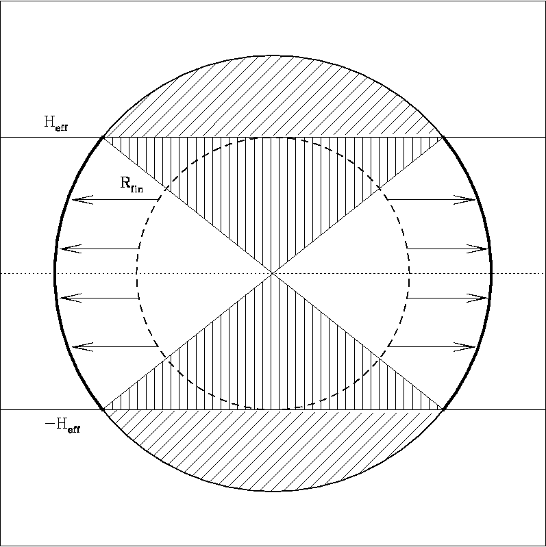
Figure 2.2: Geometrical model for blow-out. The SB starts blowing out when its radius is equal to $H_{eff}$, but continues to expand for one sound crossing time, finally reaching the radius $R_{fin}$. The two polar cups (diagonal-shaded regions), defined by the intersection of the final SB and the two planes at $H_{eff}$, are assumed to be devoid of matter. All the matter present in the double cone (vertical-shaded regions) with an aperture equal to that of the polar cups receives a radial momentum that allows it to blow-out into the halo. Taken from MO04.

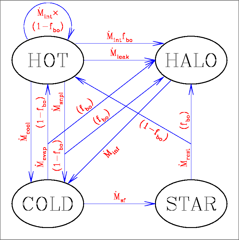
Figure 2.3: Mass flows between the four components described in the model. Arrows denote the flows connected to infall ($\dot{M}_{inf}$), star formation ($\dot{M}_{sf}$), restoration ($\dot{M}_{rest}$), cooling ($\dot{M}_{cool}$), evaporation ($\dot{M}_{evap}$), snowplows ($\dot{M}_{snpl}$), leak-out ($\dot{M}_{leak}$) and the rate at which the hot phase is engulfed by SBs ($\dot{M}_{int}$). Blow-out takes mass by a fraction $f_{bo}$ from the internal, evaporation, snowplow and restoration mass flows. Taken from MO04.

2.4.2 The system of equations

MASS FLOWS

Fig. 2.3 shows all the mass flows between the different components that are taken into account.
Cold gas continually infalls from the halo:

$$\dot{M}_{inf}=\frac{\dot{M}_{halo}}{t_{inf}}\,,$$ (2.72)

where $t_{inf}$ is the infall time-scale.
The hot phase cools at the rate $t_{cool}$, and thus the cooling mass is modelled as:

$$\dot{M}_{cool}=f_{cool}\frac{M_{hot}}{t_{cool}}\,,$$ (2.73)

where $f_{cool}$ is a free parameter regulating the fraction of the gas that is allowed to cool, while $t_{cool}$ is calculated from Eq. 2.69.
While the cold phase is easily confined even by a modest gravitational well, the hot phase is generally able to leak out of the volume $V$ to the halo. This is described as:

$$\dot{M}_{leak}=\frac{M_{hot}}{t_{leak}}\,$$ (2.74)

where $t_{leak}=\sqrt{3/d}\frac{H_{eff}}{c_{\rm s,h}}$ is the timescale connected to this leak-out, with $d$ equal to one if the leak-out is in one preferential direction, 3 if it is spherically symmetric.
The SFR is due to the contribution from the total number of collapsing clouds. Therefore cold gas is converted into stars at the rate:

$$\dot{M}_{sf}=f_{star}f_{coll}\frac{M_{cold}}{t_{dyn}}\,$$ (2.75)

A fraction $f_{rest}$ is instantaneously restored to the hot phase:

$$\dot{M}_{rest}=f_{rest}\dot{M}_{sf},.$$ (2.76)

This flux is responsible for chemical enrichment; this equation implies instantaneous recycling.
The rate at which the mass of collapsing clouds is evaporated back to the hot phase is:

$$\dot{M}_{evap}=f_{evap}\frac{\dot{M}_{sf}}{f_{\star}}$$ (2.77)

At the final time $t_{fin}$ each SB has swept a mass $M_{\rm sw}(t_{fin})$, of which a part $M_{\rm int}(t_{fin})$ is in hot internal gas and the rest $M_{snpl}$ is in the snowplow. The rate at which the hot phase becomes internal mass of a SB is:

$$\dot{M}_{int}=N_{cc}\frac{M_{\rm int}(t_{fin})}{t_{dyn}}\,,$$ (2.78)

while the rate at which it gets into a snowplow is:

$$\dot{M}_{snpl}=N_{cc}frac{M_{\rm sw}(t_{fin})-M_{\rm int}(t_{fin})}{t_{dyn}}\,.$$ (2.79)

We recall that a fraction $f_{bo}$ (Eq. 2.71) of the swept material and of the restored and evaporated mass is blown-out to the halo. If we define $\dot{M}_{bo}=f_{bo}(\dot{M}_{evap}+\dot{M}_{rest}+\dot{M}_{int}+\dot{M}_{snpl})$, the system of equations that describes the mass flows is:

$$\begin{array}[]{lcl}\dot{M}_{cold}&=&\dot{M}_{inf}+\dot{M}_{cool}-\dot{M}_{sf}-\dot{M}_{evap}+(1-f_{bo})\dot{M}_{snpl}\\ \dot{M}_{hot}&=&-\dot{M}_{cool}-\dot{M}_{snpl}-\dot{M}_{leak}-f_{bo}\dot{M}_{int}+(1-f_{bo})(\dot{M}_{evap}+\dot{M}_{rest})\\ \dot{M}_{\star}&=&\dot{M}_{sf}-\dot{M}_{rest}\\ \dot{M}_{halo}&=&-\dot{M}_{inf}+\dot{M}_{leak}+\dot{M}_{bo}\\ \end{array}$$ (2.80)

Mass conservation is guaranteed by the condition $\dot{M}_{hot}+\dot{M}_{cold}+\dot{M}_{star}+\dot{M}_{halo}=0$.

ENERGY FLOWS

We here focus on the flows regulating the energy $E_{hot}$ of the hot component, which moreover determines $T_{h}$. The total energy released by SNe is:

$$\dot{E}_{sn}=N_{cc}\frac{E_{51}N_{sn}}{t_{dyn}}$$ (2.81)

Four different processes lead to energy losses:

$$\dot{E}_{cool}=\frac{E_{hot}}{t_{cool}}\qquad\qquad\qquad\qquad\textrm{\small{COOLING}}$$ (2.82)

$$\dot{E}_{snpl}=\dot{M}_{snpl}T_{h}\frac{3}{2}\frac{k}{\mu_{h}m_{p}}\qquad\qquad\textrm{\small{SNOWPLOUGH}}$$ (2.83)

$$\dot{E}_{cool}=f_{bo}\dot{M}_{int}T_{h}\frac{3}{2}\frac{k}{\mu_{h}m_{p}}\qquad\qquad\textrm{\small{BLOWOUT}}$$ (2.84)

$$\dot{E}_{cool}=\frac{E_{hot}}{t_{leak}}\qquad\qquad\qquad\qquad\textrm{\small{LEAK-OUT}}$$ (2.85)

The energy budget of the SB $E_{sb}$ is in part given to the ISM as thermal energy, and in part as kinetic energy, which is transformed into turbulence and then partially thermalized.
The SNe feedback energy injected in the ISM is modelled according to the physical stage of the SB.
In the blow-out regime,

$$\dot{E}_{sn}=(1-f_{bo})\left(N_{cc}\frac{E^{th}_{sb}+E^{kin}_{sb}}{t_{dyn}}+\do M_{evap}T_{evap}\frac{3}{2}\frac{k}{\mu_{h}m_{\rm p}}\right)$$ (2.86)

where the first term at the right hand side models the energy the ISM received by the SB, while the second describes the energy connected to the evaporated mass.
In the adiabatic confinement regime, all the energy is given to the ISM:

$$\dot{E}_{fb}=\dot{E}_{sn}$$ (2.87)

In the PDS regime,

$$\dot{E}_{fb}=N_{cc}\frac{1}{t_{dyn}}(E^{th}_{sb}+E^{kin}_{sb}+f_{pds}E_{\rm rest})$$ (2.88)

the ISM receives the thermal and kinetic energy of the SB.
Finally, the equation regulating the energy flows in the hot component is :

$$\dot{E}_{hot}=-\dot{E}_{cool}-\dot{E}_{leak}+\dot{E}_{sb}-\dot{E}_{bo}-\dot{E}_{snpl}$$ (2.89)

In this section, we have listed the mass and energy flows implemented in the MO04 model. Describing the processes regulating the metal flows is beyond the scope of this work, we address the reader to MO04 for further reading.

In order to highlight its predictive power, MO04 ran the model in a Milky-Way-like system with the assumption that the SN bubbles are in the blow-out regime (see Sec. 2.4.1). In this case, the main characteristic of the ISM of the Galaxy are broadly reproduced, but, with respect with previous models, here parameters such as the efficiency of feedback or the Schmidt-law are consistently predicted by the model. Moreover, the MO04 model distinguishes from the previous ones because does not restrict to self-regulated, equilibrium solutions and neglects the global structure of the galaxy. It presents a rich variety of solutions with a relatively limited set of parameters. Although the turbulent nature of the ISM is not explicitly taken into account, the model is thought to give a good approximation to the solution of the feedback problem.

The MO04 model can thus construct a realistic grid of feedback solutions to be used in galaxy formation codes, either semi-analytic or numeric. For these reasons, we decided to implement the MO04 model into the GADGET-2 code (see Chapter 4).

In Monaco et al. 2007, the MO04 multiphase analytic model for supernovae feedback has been coupled to a model for the evolution of the DM haloes (thus turning into a semi-analytical model) and has been proven to be in line with the predictions of the other semi-analytical or N-body models.

2.5 Implementation and comparison of different ISM models in Gadget-2

Star formation prescriptions for numerical simulations (e.g. see previous sections for some examples) are motivated on physical grounds, and usually tested against observations of local spiral galaxies. In cosmological simulations the physical state of the star-forming gas can be very different from that of spiral galaxies: it can reside at the centre of cooling flows, forming or not forming a thin disk depending on the angular momentum content of the gas itself. The main physical difference between these two cases is the way gas is supported: in the disk case, gas is cold and dense, and its distribution is supported by its angular momentum, while in the cooling flow case the gas is partially pressure-supported. In a cosmological simulation, of course, a range of intermediate situation may and will happen. Among the many different star formation and feedback prescriptions proposed in the literature, we consider here three models that, in our opinion, give a good sampling of the possible numerical choices, namely the multi-phase effective model of SH03 (see Sec. 2.2.3), an implementation of the simple model by KA96 (see Sec. 2.3.1) and an implementation of the Thacker & Couchman 2000 prescription (TC00) that takes into account the improvement proposed by Stinson et al. 2006 (see Sec. 2.3.2). We only address feedback in the form of thermal energy, we do not consider kinetic feedback.

The TC00 model deserves some discussion: it is known to work very well for the formation of galaxy disks in cosmological simulations, so we decided to test it in non-rotating or cluster-like halos. In its original implementation, after a star formation event the algorithm distributes SN energy to all the SPH neighbours (typically 32 particles) and then disables their radiative cooling for a time $\tau$=30 Myr. This ad-hoc assumption mimics the adiabatic phase of the propagation of a SN remnant, avoiding a quick radiative loss of the deposited energy. These authors found that, compared to their previous scheme of thermal and kinetic feedback, this model allows to better conserve angular momentum of their spiral galaxies. A problem with this method is that the SPH smoothing radius, and with it the number of gas particles involved in the “adiabatic phase”, strongly depends on resolution. Stinson et al. 2006 removed this resolution-dependence problem by suitably computing how many gas particles have their cooling disabled. In Governato et al. 2007, the Stinson et al. 2006 feedback recipe was used in a cosmological simulation of a disk galaxy and was proven to be very efficient in reducing the loss of angular momentum: this feedback model produces more extended disks with smaller bulges and the right trend of star formation history with galaxy mass. Besides, the simulated galaxies lie close to the observed baryonic Tully-Fisher relation.

2.5.1 Numerical methods

We use the GADGET-2 code, a parallel Tree+SPH code (Springel 2005) with a fully adaptive time-step algorithm. The version of the code that we use adopts an SPH formulation with entropy conserving integration and arithmetic symmetrisation of the hydrodynamical forces (SH03), and includes radiative cooling computed for a primordial plasma with vanishing metalicity.

As mentioned in the Introduction, we address three different star formation and feedback models. The first one is the original GADGET-2 effective model for star formation and feedback (EFF). It is based on a simple model for the multi-phase structure of the star-forming gas on the small scales which are not resolved in cosmological simulation. The second one (simple star formation, SSF) is an implementation of that described in KA96, a single-phase model for star formation and SNe feedback which is described in Sec. 2.3.1. The third one is an implementation of Stinson et al. 2006, starting from SSF, consists in turning off radiative cooling for a fixed amount of time after a star formation episode (delayed cooling, DEL).

For simplicity, we do not consider any type of kinetic feedback, because none of the schemes we use has a self-consistent prescription for it, so it would be implemented as an independent prescription applied on top of the sub-grid model. The EFF, SSF and DEL models have been previously presented in Sec. 2.2.3, Sec. 2.3.1 and Sec. 2.3.2. In the following, we adopt values of $\rho_{\rm tr}$ corresponding to a number density of $n_{\rm thr}$=0.25 cm${}^{-3}h^{-3}$ and $T_{\rm thr}$= $2\cdot 10^{4}$ K .

2.5.2 Simulations

We run simulations with the three star formation and feedback models for three configurations, two isolated, non-rotating halos and a cosmological cluster-sized halo.

For the two isolated halos, we set up initial conditions for our models as in Viola et al. 2008, considering objects whose DM component has a Navarro, Frenk & White (1996, 1997) density profile. Gas pressure is computed using the universal gas-density and temperature profiles derived by Komatsu & Seljak 2001. They make three assumptions: (1) the gas is in hydrostatic equilibrium within the gravitational potential of the DM halo (as described in Suto et al. 1998; (2) the slopes of the DM and gas density profiles are equal at the virial radius, thus fixing the gas thermal energy; (3) the gas follows a constant polytrophic equation of state; we use the value $\gamma_{p}$=1.18, for the effective polytrophic index. Initial positions of DM and gas particles are assigned by Monte-Carlo sampling the analytical density profiles of DM and gas. To create an equilibrium configuration for the DM halo, we assign initial velocities of the DM particles by assuming a local Maxwellian approximation (Hernquist 1993). The width of the distribution, which gives the velocity dispersion of the DM particles, is obtained by solving Jeans’ equation. Regarding gas particles, because the gas is in hydrostatic equilibrium, particles are assigned zero velocities and their internal energy is set according to the computed temperature profile. This procedure allows to generate configurations that are in approximate equilibrium, so, before switching on cooling, star formation and feedback, we let the system evolve for two dynamical times, so as to start from a truly relaxed state.

With this procedure we generate two halos, having masses of $10^{13}$ $h^{-1}{\rm M}_{\odot}$, typical of a $z$=0 poor galaxy group, and $10^{12}$ $h^{-1}{\rm M}_{\odot}$, typical of an isolated galaxy. Virial radii are computed as $r_{200}$, the radius for which the average density is 200 times the critical density at $z$=0. Concentrations of the two halos are chosen respectively as $c_{\rm NFW}$=6.3 and $c_{\rm NFW}$=7.25, given by the relation between mass and concentration provided by NFW (1997). Both halos are sampled with 6 x $10^{4}$ DM and gas particles inside $r_{200}$; the profiles are extrapolated to several virial radii so as to have pressure support at the virial radius. We assume the baryon fraction to be $f_{\rm bar}$=0.19. We set the Plummer-equivalent softening to be $2.64\ h^{-1}$ kpc, the value suggested by Power et al. 2003, for Me12.

For Me13, we rescale the softening to $5.7\ h^{-1}$ kpc. We assume the minimum value for the SPH smoothing length to be 0.5 times that of the gravitational softening; we also set the number of the SPH neighbours $N_{\rm ngb}$ to be 32. In all runs we set the initial angular momentum to zero. The main characteristics of these halos are summarised in Table 2.1. Since the overdensity used to define the virial radius is constant ($\Delta\rho=200\rho_{c}$), $t_{\rm dyn}$ (Eq. 2.35) takes a value of 0.56 Gyr for both halos.

We evolve Me12 for 4 dynamical times and Me13 for 8 dynamical times; the difference is due to the longer time needed by the larger object to reach a similar evolutionary stage when compared with the smaller one.

The third configuration used in this paper is a DM halo taken from a cosmological simulation. We use the initial conditions of the object labelled CL4 of Borgani et al. 2006 at the “medium” resolution: the mass of a DM particle is $1.5\cdot 10^{9}$ $h^{-1}{\rm M}_{\odot}$, the mass of a gas particle is $2.3\cdot 10^{8}$ $h^{-1}{\rm M}_{\odot}$, and the Plummer-equivalent softening is $5$ $h^{-1}$ proper kpc from $z$=0 to $z$=2 and is kept fixed in comoving coordinates for $z$$>$2. The background cosmology is a flat $\Lambda$CDM cosmological model with $\Omega_{m}$=0.3, $h$=0.7, $\sigma_{8}$=0.8 and $\Omega_{b}$=0.04. The initial conditions were produced using the Zoomed Initial Condition technique (Tormen et al. 1997; see Borgani et al. 2006 for further details). At redshift $z$=0, our selected cluster has a mass of $\approx 1.6\cdot 10^{14}$ $h^{-1}{\rm M}_{\odot}$ within $R_{\rm vir}\approx 1.1$ $h^{-1}$ Mpc, defined as the radius enclosing an overdensity of $\approx 100$ times the critical density, as predicted by the spherical collapse model in our assumed cosmology. It therefore contains $\approx 9\cdot 10^{4}$ DM and gas particles, a number which is comparable to that adopted for our isolated runs. In the spirit of this work, in this cosmological run we do not model SNIa, kinetic feedback, metalicity of the gas and metal cooling. We only keep into account the effect of a uniform redshift-dependent UV radiation background (Haardt & Madau 1996).

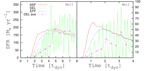
Figure 2.4: SFRs as a function of time (in units of $t_{\rm dyn}$) for simulations of isolated halos with the three studied models: EFF (short-dashed line), SSF (solid line) and DEL (long-dashed).The left panel shows Me13 SFRs up to $8t_{\rm dyn}$ and the right panel the Me12 SFRs up to $4t_{\rm dyn}$(see text). We resampled the Me13 and the Me12 DEL SFRs (dotted line) with a constant time interval equal respectively to 0.13 $t_{\rm dyn}$ and 0.08 $t_{\rm dyn}$.

	$M_{200}$	$r_{200}$	$c_{\rm NFW}$	$m_{\rm DM}$	$m_{\rm gas}$
Me13	$10^{13}$	350	6.3	$1.3\cdot 10^{8}$	$3.1\cdot 10^{7}$
Me12	$10^{12}$	162	7.25	$1.3\cdot 10^{7}$	$3.1\cdot 10^{6}$
CL4	$1.6\cdot 10^{14}$	1100	—	$1.5\cdot 10^{9}$	$2.3\cdot 10^{8}$

Table 2.1: Main properties of the simulated halos. In all runs, we used 6*$10^{4}$ DM particles and as many gas particles inside $r_{200}$. Column 1: halo name. Column 2: mass enclosed in within $r_{200}$ in $h^{-1}{\rm M}_{\odot}$. Column 3: value of $r_{200}$ in $h^{-1}$ kpc. Column 4: NFW concentration. Column 5: mass of a DM particle in $h^{-1}{\rm M}_{\odot}$. Column 6: mass of a gas particle in $h^{-1}{\rm M}_{\odot}$.

2.5.3 Results

In this Section we compare SFRs, phase diagrams, density and temperature profiles obtained simulating our Me13, Me12 and CL4 halos with the EFF, SSF ad DEL star formation and feedback schemes described above.

Run	EFF	SSF	DEL
Me13 ($4t_{\rm dyn}$)	0.07	0.08	0.01
Me12 ($4t_{\rm dyn}$)	0.33	0.35	0.08
Me13 ($8t_{\rm dyn}$)	0.22	0.23	0.08
CL4 ($z$=0)	0.27	0.25	0.19

Table 2.2: Gas cold fraction (mass of stars over mass of baryons) for Me13 and Me12 within $r_{200}$ and for CL4 within $r_{vir}$. We show results for Me13 and Me12 at $4t_{\rm dyn}$, Me13 at $8t_{\rm dyn}$, CL4 at $z$=0.

Isolated halos: star formation rates

In Fig. 2.4 we show SFRs for EFF, SSF, and DEL simulations of the two isolated halos Me13 and Me12, evolved for $8t_{\rm dyn}$, and $4t_{\rm dyn}$ respectively.

Regarding Me13 (left panel), in both EFF and SSF schemes star formation starts after $\approx 1.3t_{\rm dyn}$, when the cooling flow is established and the gas in the central part of the objects is dense and cold enough to become star-forming. The behaviour of star formation in these two schemes is similar, with SSF forming $\approx$10% more stars than EFF. At $6t_{\rm dyn}$, a similar SFR of slightly less than $\approx$150 M_⊙ yr^-1 is achieved, slowly declining with time while the gas is consumed. Feedback in the EFF scheme is thus only slightly more efficient than in the SSF one, and this causes a slightly slower rise of star formation.

The DEL scheme shows a different behaviour. The SFR grows much more slowly than in EFF and SSF schemes, and at $4t_{\rm dyn}$ it is still 30% lower on average, reaching the other two curves at At 8$t_{\rm dyn}$. Clearly, the DEL scheme is efficient in suppressing star formation in this object. But the most noticeable property of this SFR curve is that it is intermittent and spiky.

The right panel of Fig. 2.4 shows the SFRs for Me12. Also in this case, the onset of star formation is quicker for the SSF scheme, and the SFR is $\approx$25% higher in SSF than in EFF at its peak. After $2t_{\rm dyn}$ the EFF and SSF schemes do converge to the same SFR, which then decreases with time. Again, DEL shows an intermittent behaviour, and, on average, a much slower rise in SFR; it reaches the SFR of the other two schemes, on average, only after $3t_{\rm dyn}$; later on, oscillations are visible even for the average value of the star formation curve.

Note that EFF and SSF SFRs converge for Me13 and Me12 at different times. The dynamical time of the halos is the same, but the cooling times are shorter for Me12 and thus its evolution is faster.

The spiky behaviour of star formation in the DEL scheme is due to the fact that many particles simultaneously cool down and reach the star formation threshold at the same time. These particles spawn stars simultaneously, getting energy and stopping from cooling. All the star-forming gas is thus prevented from further star-forming for 30 million years. After that time gas cools and condenses, crosses again the threshold and the cycle is repeated, involving new gas which has cooled in the meanwhile.

Cold fractions (defined as the mass in stars divided by the total baryon mass within the virial radius) for the three schemes in the Me13 and Me12 cases after 4 $t_{\rm dyn}$ are listed in Table 2.2, where we also list the cold fractions after 8 $t_{\rm dyn}$ for Me13. Consistently with what discussed above, SSF scheme is the most efficient model in converting gas into stars, EFF scheme in only slightly less efficient. On the other hand, due to its intermittent behaviour, cold fractions in DEL model are very low, about one tenth of EFF and SSF in the Me13 case and about one quarter in Me12 at the end of the simulations.

These results confirm the well-known result that thermal feedback is not efficient in models like EFF and SSF, while the DEL model is very effective at suppressing star formation, but at the cost of a strongly intermittent behaviour.

Isolated halos: thermodynamics

To achieve a better physical understanding of the differences among our three feedback schemes, we investigate the phase diagrams ($\rho$ versus $T$) of gas particles We use the effective temperature for the EFF scheme, since it is the pertinent one as far as hydrodynamics is concerned.

Fig. 2.5 and 2.6 show phase diagrams for the Me13 and Me12 halos. We show both halos for sake of completeness, but all conclusions that are drawn from Me13 are confirmed by Me12, so we will concentrate on the more massive halo. The upper left panel of Fig. 2.5 shows the phase diagram for Me13 with the EFF model after $4t_{\rm dyn}$. Here we only consider gas particles lying in the inner 20 $h^{-1}$ kpc of the halo. This diagram is populated in two main regions: hot, low-density particles flowing toward the halo centre (the cooling flow) populate the upper-left corner, denser and colder particles, the ones in the multi-phase regime, are visible in a tight relation at $T\sim 10^{5}$ K. Only a few particles join the two regions, tracing a cooling path at intermediate densities and temperatures. The effective temperature of the star-forming gas particles is set by the weighted average of the hot phase energy (given by Eq. 2.30) and the cold phase energy (which is fixed), so it is higher than $T\approx 10^{4}$ K, which is where the cooling function drops, and is a function of the density through the multi-phase model. This density-temperature relation is sharply truncated at the density where the probability of spawning a star becomes nearly unity. Because particles heated by feedback would populate the upper-right corner of this diagram, this demonstrates that, in absence of kinetic winds, feedback in the EFF model only acts in rising the temperature of the star-forming particles.

The upper right panel of Fig. 2.5 shows the same plot for the SSF scheme. This time the star-forming particles cool down to $\approx 10^{4}$ K; due to the short cooling times at such high densities, SN energy given to gas particles is almost completely uneffective at populating the upper-right corner of the diagram.

The lower panels shows two phase diagrams for the DEL scheme. For Me13 we have chosen two different times: $t=3.8t_{\rm dyn}$ (lower left panel), corresponding to a phase of quenched star formation, and $t=4t_{\rm dyn}$ (lower right panel), corresponding to a peak of star formation. For Me12, shown in Fig. 2.6, the chosen times are $t=3.6t_{\rm dyn}$ and $t=3.9t_{\rm dyn}$. Consistently with the SFRs, at $3.8t_{\rm dyn}$ all particles in the Me13 halo have temperatures higher than the threshold for forming stars, while at $4t_{\rm dyn}$ a large number of particles are dense and cold enough to form stars. At the later time a column of particles with very high density and high temperatures, spanning the range $10^{5}<T<3\cdot 10^{6}$ K, is visible. These particles have just acquired energy from a star formation episode. The acquired energy varies depending on whether the same particle or a neighbour has spawned a star. The $4t_{\rm dyn}$ diagram also shows the trajectory of a single gas particle. This starts at the leftmost end, with high temperature and low density. It cools down to $T\sim 10^{4}$ K and spawns a stars. As a consequence it is heated up to $\sim 10^{6}$ K; a phase of adiabatic expansion follows, caused by the fact that the particle has its cooling stopped. At the final time of the trajectory, $t=4t_{\rm dyn}$, cooling is switched on again. This shows that the heated particles, adiabatically expanding and then cooling, occupy the region at relatively high densities, between $5\cdot 10^{7}$ and $5\cdot 10^{8}$ $h^{2}$ M_⊙ kpc^-3, and temperatures between $10^{5}$ and a few times $10^{6}$ K. During the cooling phase of the particle its trajectory in the phase diagram shows a “bump” in which both temperature and density rise. This is due to a weak shock caused by its interaction with high-density particles which are adiabatically expanding. These weak shocks cause the density to increase gradually after each star formation burst. Indeed, Fig. 2.5 shows that DEL star-forming particles have higher densities than EFF and SSF ones.

In the outer part of the halo, the phase diagram of Me13 (Fig. 2.5) do not show any difference among the three schemes, confirming that in such relatively massive halos differences in star formation and feedback do influence only the very inner, star-forming region. This is different in the less massive Me12 halo (Fig. 2.6), where the DEL feedback model shows some influence on the external parts.

Figure 2.5: Phase diagrams ($T$ versus $\rho$) for gas particles of Me13 simulations. Only particles in the inner 20 $h^{-1}$ kpc are shown. Upper panels show the EFF (left) and SSF (right) models at $4t_{\rm dyn}$. Lower panels show the DEL model at $3.8t_{\rm dyn}$ (left) and $4t_{\rm dyn}$ (right).

Figure 2.6: Phase diagrams ($T$ versus $\rho$) for the gas particles for Me12 after. Panels are as in Figure 2.5; lower panels are at $3.6t_{\rm dyn}$ (left) and $3.9t_{\rm dyn}$ (right).

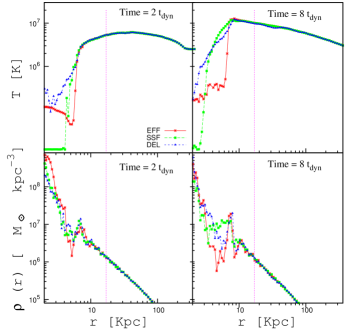
Figure 2.7: Me13 gas density (bottom panels) and temperature (top panels) profiles at $2t_{\rm dyn}$ (left) and $8t_{\rm dyn}$ (right) for the three models studied. The vertical line marks the scale corresponding to three softening lengths.

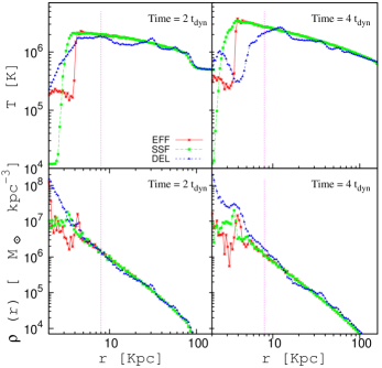
Figure 2.8: Me12 gas density (bottom panels) and temperature (top panels) profiles at $1t_{\rm dyn}$ (left) and $4t_{\rm dyn}$ (right) for the three models studied. The vertical line marks the scale corresponding to three softening lengths.

In Fig. 2.7 we show gas temperature (effective temperature for the EFF model) and density profiles for the Me13 case after $2t_{\rm dyn}$, when all SFRs are still growing and differences among models are more marked, and $8t_{\rm dyn}$, where models give convergent values. The vertical line marks three softening scales; smaller structures are not properly resolved.

No significant differences among the three models are visible at the scales that are well resolved in this simulation. At small distances temperatures drop to $10^{4}$ K in the SSF and to $\sim$$10^{5}$ K both for EFF and DEL, in the first case as the effect of the multi-phase model, in the second case as an effect of the delayed cooling. The density profiles show that at sub-softening scales DEL density is higher than the other two models, consistently with what inferred from the phase diagrams.

Analogously to Fig. 2.7, Fig. 2.8 shows temperature and density profiles for the Me12 halo at $2$ and $4t_{\rm dyn}$. The general behaviour is similar to the Me13 case, with the difference that wiggles are present in the DEL profiles. These are compression waves propagating through the outer halo as a consequence of the efficient and intermittent energy injection from SNe. These are not visible in the more massive Me13 halo, which is also characterised by a higher virial temperature.

In conclusion, the most relevant differences among models are restricted to the central, sub-softening regions where star formation occurs. The effects of stellar feedback are visible on the halo gas component only for the smaller halo and for the efficient feedback scheme. This is in line with the well-known finding that stellar feedback cannot influence the thermodynamics of the intra-cluster medium (Borgani et al. 2004, Kay et al. 2007, Nagai et al. 2007).

We also performed several numerical tests on our isolated halos, to assess the stability of our results with respect to the details of the implementation and to the resolution. In particular, we verified on the Me13 halo that using 10 times more particles does not change either the intermittent behaviour of the star formation rate in the DEL case or its low star formation efficiency. Therefore, also with higher resolution, the star formation is delayed when compared with the EFF scheme.

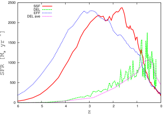
Figure 2.9: SFRs as a function of redshift in $t_{\rm dyn}$ for the cosmological CL4 simulations with the three models studied. Symbols are as in Figure 2.4.

Cosmological case

Fig. 2.9 shows the SFRs for the CL4 cluster. For the EFF, SSF and DEL models, star formation peaks respectively at redshift $z$$\sim$3 $\sim$1.7 and $\sim$0.7. Regarding this last model, the typical spiky SFR is visible only at low redshift, and this is due to the fact that star formation at high redshift is averaged over many progenitors; when, at low redshift, the most massive progenitor dominates the mass distribution, the spiky character of the star formation becomes visible.

Cold fractions at $z$=0 for the three cases are reported in Table 2.2: SSF and EFF lock many baryons (27% and 25%) in the stellar component, while DEL gives a lower figure of $\sim$19%.

Fig. 2.10 and 2.11 show density and temperature profiles at four different redshifts, $z$=2, $z$=1, $z$=0.5 and $z$=0. In this last case no significant differences among the three models are visible at scales larger than three softening lengths. As far as the inner, poorly resolved region is concerned, at low redshift (0 and 0.5) the gas density is lower for EFF and SSF than the DEL cases, simply because more gas has been transformed into stars in the two models. More marked differences are visible at higher redshift (1 and 2) even at resolved scales up to $\sim$40 $h^{-1}$ kpc, especially in the temperature profiles: they clearly show the signature of the different star formation prescriptions used. The behaviour of temperature profiles is overall similar to that shown by the isolated cases, with SSF having cold star-forming gas, EFF having warmer gas with temperatures given by the effective model, and DEL showing the hottest temperature. Moreover, DEL influences the temperature profile to several tens of kpc, in a way that resembles Me12 (Fig. 2.8). Indeed, at such high redshift the mass of the main progenitor is still $\sim 3\cdot 10^{13}h^{-1}$ $h^{-1}{\rm M}_{\odot}$, but with a higher average density that enhances the effect of feedback.

In most cases differences are limited to sub-softening scales, and no relevant difference is visible in any case beyond 50 $h^{-1}$ kpc; moreover, no star formation and feedback model produces a roughly isothermal “cool” core: the temperature peaks at $\sim 20-60\ h^{-1}$ kpc and drops to low values at smaller radii. This is in line with the well-known result that no stellar feedback scheme is able to significantly influence the intra-cluster medium at large scales.

The DEL feedback scheme is able to influence the ICM at some tens of kpc, and to limit the fraction of cold baryons from $\sim$25%, which is incompatible with the typical 10% value of clusters (Balogh et al. 2001, Lin et al. 2003), to a lower value of 19%. However, this is obtained at the cost of severely suppressing star formation at high redshift and moving the peak of SFR to a very low redshift. This is incompatible with the estimated age of cluster galaxies, which form the bulk of their stars at $z>2$.

Other groups, e.g, Governato et al. 2007, didn’t find unrealistic star formation histories when using SF schemes similar to our DEL one. The main difference with our result, is that they simulate the cosmological formation of a galaxy-sized halo, characterised by an early formation epoch and a high spin parameter. The gas there is shock-heated at high redshift, then it cools down and settles in a rotation-supported cold disk with low SFR and consequently a low level of feedback. For a cluster-sized halo, merging is active up to low redshift and no rotation-supported disk forms. As a consequence, the behaviour typical of our non-rotating isolated halos is the predominant one and this causes an unrealistically delayed star 60.

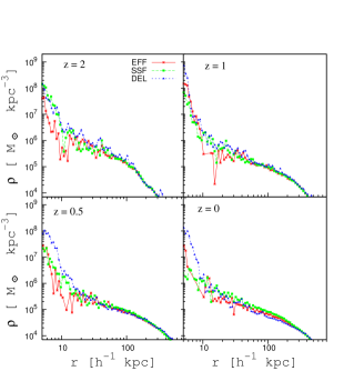
Figure 2.10: Evolution of the gas density in the cosmological run for the three models studied. The vertical line marks the scale corresponding to three softening lengths.

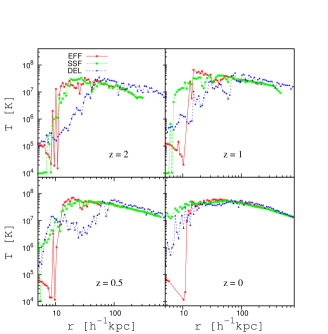
Figure 2.11: Evolution of the gas temperature in the cosmological run for the three models studied. The vertical line marks the scale corresponding to three softening lengths.

2.5.4 Conclusions

In this section, we presented a comparison of different star formation and SNe feedback prescriptions in NFW isolated, non-rotating DM halos of mass $10^{13}$ and $10^{12}$ $h^{-1}{\rm M}_{\odot}$ and in a $1.6\cdot 10^{14}$ $h^{-1}{\rm M}_{\odot}$ cosmological DM halo, using the TREE+SPH code GADGET-2. Usually, such tests of star formation models are performed on disk galaxies, where gas is rotation-supported. Our settings are remarkably different: in our isolated halos a cooling flow is established soon after the beginning of the simulation, and gas is pressure-supported when it is not falling to the centre of the halo. This is similar to what happens in a galaxy cluster, like in our cosmological case. So this represents a complementary test with respect to the standard disk formation tests.

We chose to test the GADGET effective model (EFF, SH03), which is based on a multi-phase description of the gas contained in a particle, an implementation of the scheme proposed by Katz et al. 1996 (SSF, KA96), where feedback energy is given to star-forming particles in the form of thermal energy, and an implementation of Thacker & Couchman 2000 with the improvements of Stinson et al. 2006 (DEL). In this last scheme, after a star formation event, the gas gains energy from SNe explosions and cooling is quenched for a fixed period of time of 30 Myr. For simplicity, we did not consider feedback in the form of kinetic energy.

Our main conclusions are:

• In the EFF and SSF models thermal feedback is inefficient and unable both to limit star formation and to influence the gas dynamics beyond the gravitational softening scale.

• In isolated non-rotating halos, the effect of delaying radiative cooling in a cooling flow is to drastically reduce the amount of formed stars. This happens because the simultaneous cooling of a large amount of gas triggers an intermittency in star formation, with intense episodes followed by periods in which the whole gas is heated up and no star formation is allowed.

• Delaying radiative cooling in a cooling flow when using thermal feedback has little effect on the thermodynamics of the intra-cluster medium at length scales larger than some softening lengths, as expected. Temperature and density profiles do not differ much between runs with delayed and normal cooling. For the smaller isolated halo and for the cosmological halo at moderately high redshift, compression waves are visible in the temperature profiles; they are signatures of the intermittent star formation behaviour.

• A cosmological simulation of formation and evolution of a $\sim 10^{14}$ $h^{-1}{\rm M}_{\odot}$ galaxy cluster, using the DEL scheme, shows trends in SFRs, cold fractions and density and temperature profiles which resembles the one we obtained in our isolated cases.

• In the cosmological simulation, in particular, the peak in the star formation history for the DEL scheme is at a redshift $z<1$, in disagreement with observations. The cold fraction is instead relatively low, 19% at redshift $z$=0; this is due to the late star formation.

• No model is able to produce a roughly isothermal core like those observed in cool-core clusters.

• EFF and SSF schemes gives very similar result also in the cosmological test case with too much gas locked in the stellar component.

We conclude that, while SN feedback in EFF and SSF schemes are not efficient in countering the cooling flow and gas radiative losses at the halo centre, the DEL scheme proves extremely effective at doing so. The cost of it is an unrealistic delay in the star formation history. While star formation and feedback schemes which turn off radiative cooling have proved to be effective at producing realistic disk galaxies in cosmological simulations, caution should therefore being used when utilising similar schemes as general-purpose ones.

Chapter 3 The origin of IntraCluster stars in cosmological simulations of galaxy clusters

Observations of diffuse intracluster light and individual intracluster stars in nearby clusters (Arnaboldi et al. 2002, Arnaboldi et al. 2003, Arnaboldi et al. 2004, Feldmeier et al. 2003, Mihos et al. 2005, Gerhard et al. 2005) and at intermediate redshift (Gonzales et al. 2000, Feldmeier et al. 2004, Zibetti et al. 2005) indicate that a substantial fraction of stars becomes unbound from galaxies as these fall towards the densest parts of their cluster environment.

The radial distribution of the intracluster light (ICL) in galaxy clusters is observed to be more centrally concentrated than that of the cluster galaxies (Zibetti et al. 2005), a result which was predicted from cosmological hydrodynamical simulations of galaxy clusters (Murante et al. 2004, M04 hereafter). Zibetti et al. 2005 also find that the surface brightness of the ICL correlates both with BCG luminosity and with cluster richness, while the fraction of the total light in the ICL is almost independent of these quantities. Other observations indicate an increase of the relative fraction of diffuse stars from the mass scale of loose groups (less than 2 %, Castro-Rodríguez et al. 2003, Feldmeier et al. 2003) to that of Virgo-like clusters ($\approx 5-10$% Feldmeier et al. 2003, Arnaboldi et al. 2003, Mihos et al. 2005) up to the most massive clusters (10-20 % or higher Gonzales et al. 2000, Feldmeier et al. 2002, Gal-Yam et al. 2003, Feldmeier et al. 2004, Krick et al. 2006).

The origin and evolution of this diffuse stellar component (DSC) is currently unknown and several mechanism are being investigated. The ICL may be produced by stripping and disruption of galaxies as they pass through the central regions of relaxed clusters (Byrd $\&$ Valtonen 1990, Gnedin 2003). Other mechanisms are the stripping of stars from galaxies during the initial formation of clusters (Merritt 1984); creation of stellar halos in galaxy groups, that later fall into massive clusters, and then become unbound (Mihos 2004, Rudick et al. 2006); stripping of stars during high–speed galaxy encounters in the cluster environment (Moore et al. 1996). Evidence for ongoing stripping from elliptical galaxies in clusters was presented by Cypriano et al. 2006.

In parallel, numerical simulations have been performed to investigate the properties the DSC in galaxy clusters within the current cosmological models. Napolitano et al. 2003 used Dark-Matter (DM) only simulations, and identified the stellar component using the DM particles as tracers. For the first time, M04 used a $\Lambda$CDM cosmological hydrodynamical simulation, including radiative cooling and star formation, to quantify the amount and the distribution of the DSC in a set of 117 clusters. Willman et al. 2004 and Sommer-Larsen et al. 2005 found a DSC in their simulated single clusters. Willman et al. 2004 discussed the origin of the DSC: they found a correlation between the cluster growth and the increase in the DSC mass, and that both massive and small galaxies contribute to its formation.

Recently, Rudick et al. 2006 performed collisionless simulations where high–resolution model galaxies were inserted in their dark matter halos at a given redshift, and then their common evolution in a cluster was followed from that time on. A DSC was formed, and Rudick et al. 2006 found that the cluster DSC grows with the accretion of groups during the cluster history.

In this work, we focus on the formation mechanism of the ICL in a cosmological hydrodynamical simulation (Borgani et al. 2004, M04). The formation of galaxies and their subsequent dynamical evolution in a time dependent gravitational potential is a direct consequence of the hierarchical assembly process of cosmic structures. Using a large ($192^{3}h^{-3}$ Mpc³) volume simulation, we study a statistically significant ensemble of galaxy clusters and follow how stars become unbound from galaxies during the evolution of clusters as a function of cosmic time. We also address the stability of our results against numerical resolution by carrying out the same analysis on three clusters from this set, which were re-simulated at a substantially improved force and mass resolution.

The plan of the paper is as follows: in Section 3.1 we describe our numerical simulations and in Section 3.2 we give details on the galaxy identification and properties. In Section 3.3 we describe the identification of the diffuse stellar component (DSC). In Section 3.4 we present the link between galaxy histories and the formation of the DSC; in Section 3.5 we discuss how resolution and other numerical effect may affect our results; in Section 3.6 we discuss the dynamical mechanisms that unbind stars from galaxies in clusters and compare with the statistical analysis of the cosmological simulation performed in the previous Sections. In Section 3.7 we summarise our results and give our conclusions.

3.1 The simulated clusters

The clusters analysed in this paper are extracted from the large hydrodynamical simulation (LSCS) of a “concordance” $\Lambda$CDM cosmological model ($\Omega_{m}=0.3$, $\Omega_{\Lambda}=0.7$, $\Omega_{\rm b}=0.019\,h^{-2}$, $h=0.7$ and $\sigma_{8}=0.8$). This simulation is presented in Borgani et al. 2004 and we refer to that paper for additional details. The LSCS is carried out with the massively parallel Tree+SPH code GADGET2 (Springel et al. 2001, Springel 2005), and follows $480^{3}$ dark matter particles and as many gas particles in a periodic box of size $192\,h^{-1}$ Mpc. Accordingly, the mass resolution is $m_{\rm dm}=4.6\times 10^{9}\,h^{-1}M_{\odot}$, $m_{\rm gas}=6.9\times 10^{8}h^{-1}M_{\odot}$ and $m_{\rm star}=3.465\times 10^{8}h^{-1}M_{\odot}$. The Plummer–equivalent softening length for the gravitational force is set to $\epsilon=7.5\,h^{-1}$ kpc, fixed in physical units from $z=0$ to $z=2$, while being fixed in co-moving units at higher redshift. The SPH softening length of the gas is allowed to shrink to half the value of the gravitational force softening. The simulation includes radiative cooling, the effect of a photo–ionising uniform UV background, star formation using a sub-resolution multi-phase model for the interstellar medium (Springel & Hernquist 2003), feedback from supernovae (SN) explosions, including the effect of galactic outflows. The velocity of these galactic winds is fixed to $v_{w}\simeq 340\,{\rm km\,s^{-1}}$, which corresponds to 50$\%$ efficiency for SN to power the outflows.

Clusters are identified at $z=0$ using a standard friends-of-friends (FOF) algorithm, with a linking length of $0.15$ times the mean dark matter inter-particle separation. We identify 117 clusters in the simulation with $M_{FOF}>10^{14}h^{-1}M_{\odot}$. Cluster centres are placed at the position of the DM particle having the minimum value of the gravitational potential. For each cluster, the virial mass $M_{\rm vir}$ is defined as the mass contained within a radius encompassing an average density equal to the virial density, $\rho_{\rm vir}$, predicted by the top–hat spherical collapse model. For the assumed cosmology, $\rho_{\rm vir}\simeq 100\rho_{c}$, where $\rho_{c}$ is the critical cosmic density (e.g. Eke et al. 1996).

To test the effects of numerical resolution on the final results, we select three clusters, having virial masses $M_{\rm vir}=1.6,2.5,2.9\times 10^{14}h^{-1}$M_⊙, and re-simulate them twice with different resolution. While the first, lower-resolution simulation is carried out at the same resolution as the parent simulation, the second simulation had a mass resolution $45\times$ higher, with a correspondingly smaller softening parameter, $\epsilon=2.1\,h^{-1}$ kpc. These re-simulations are performed using more efficient SN feedback, with a wind velocity $v_{w}\simeq 480\,{\rm km\,s^{-1}}$. A detailed description of these re–simulations is provided by Borgani et al. 2006.

3.2 Identifying galaxies in a cluster with SKID

The identification of substructures inside halos is a longstanding problem, which is not uniquely solved. In the present work, we need to identify galaxies in the simulations from the distribution of star particles which fill the volume of the cosmological simulation.

In the LSCS, “galaxies” are defined as self—bound, locally over-dense structures, following the procedure in M04, which is based on the publicly available SKID algorithm (Stadel 2001). At a given redshift, once the star particles have been grouped by SKID, we classify as galaxies only those groups which contain at least 32 bound star particles. There is a degree of uncertainty in the galaxy identification by SKID, as in other similar identification algorithms, which comes in from the assignment of those star particles which are located in its outskirts of each self-bound object. The main advantage of this identification algorithm is that it provides a dynamically–based, automated, operational way to decide whether a star particle belongs to a gravitationally bound object or not. Additional details of the galaxy identification algorithm and on our tests are given in the Appendix.

We expect that, once a self-bound structure of luminous particles has been formed at a given redshift, most of its mass will remain in bound structures, for all subsequent redshifts. However, it may happen that a group of particles classified as a “galaxy” at one output redshift, with a number of particles just above the specified minimum particle threshold for structure identification, may fall below this limit at the next redshift output. This may occur, for example, because the group is evaporated by interaction with the environment. Following Springel et al. 2001, we call structures that can be identified only at one output redshift volatile, and do not consider them further.

All star particles that never belong to any galaxies identified in the selected redshift outputs are also assigned to this volatile class. Such star particles either do not belong to any bound structure already at the first output redshift, at $z=3.5$, or they form in a galaxy and become unbound between two simulation output redshifts. In both cases, since we cannot assign those stars to the history of any galaxies, we cannot determine their dynamical origin.

An important issue in our study concerns the reliability of the simulated galaxy population. If galaxies are under-dense, they can easily lose stars or be completely disrupted as a consequence of numerical effects. In simulations, low-mass galaxies may have typical sizes of the order of the adopted softening parameter, so that their internal mass density is underestimated. Therefore at the low-mass end, we expect that our simulated galaxies will have an internal density which is an increasing function of galaxy mass. On the other hand, numerical effects should be less important for the more massive galaxies.

To investigate this issue, we evaluate the stellar density of all the simulated galaxies at the half-mass-radius, and plot these in Figure 3.1 as a function of the galaxy mass, combining all redshift outputs.

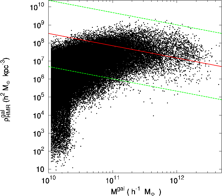
Figure 3.1: The mean galaxy stellar density inside the half-mass-radius as a function of galaxy mass. All galaxies identified in the parent simulation at all 17 redshift outputs areshown. The solid line shows an estimate of the observed galaxy densities from SDSS data (see text). The dotted lines show the densities corresponding to the $3\sigma$ scatter reported in Shen et al. 2003.

For real galaxies, the internal density of (early–type) galaxies is a decreasing function of their mass, as shown most recently by Shen et al. 2003, who measured the size distribution for 140,000 galaxies from the Sloan Digital Sky Survey. We use their measured size distribution to estimate the observed galaxy densities within the half-mass-radius. For this purpose, we take the expressions for a Hernquist profile in Hernquist 1990 to relate Sersic half-light radii to three-dimensional half-mass radii, and then convert the Sersic size-stellar mass relation for early-type galaxies of Shen et al. 2003 to a relation between stellar mass and mean density within the half-mass radius. The solid line in Fig. 3.1 represents the resulting estimate of the mean galaxy density, with the dotted lines limiting the $3\sigma$ scatter of the size distribution as reported in Shen et al. 2003. The dots in Fig. 3.1 show the equivalent mean densities of our simulated cluster galaxies. In what follows, we use the lower $3\sigma$ envelope to estimate the minimum acceptable galaxy densities $\rho_{\rm min}(M_{\rm gal})$. Galaxies with density lower than this minimum density are discarded and also classified as volatile. From Fig. 3.1 we note that the observed trend of decreasing density with increasing mass is recovered in our (lower-resolution) parent simulation for galaxy masses $\raise-2.0pt\hbox{\hbox to0.0pt{\hbox{$\sim$}\hss}\raise 5.0pt\hbox{$>$}\ }10^{11}h^{-1}M_{\odot}$.

In order to quantify the effect of volatile galaxies on our final results, we tested other density thresholds, namely (i) one corresponding to $1\sigma$ scatter in the $R_{e}$ distribution, (ii) a fixed value of $\rho=5\cdot 10^{6}h^{2}M_{\odot}$/kpc³, as well as (iii) a galaxy mass threshold, $M=6\cdot 10^{10}h^{-1}M_{\odot}$. Our results remain qualitatively unchanged when either of these criteria is adopted.

3.3 Identifying the Diffuse Stellar Component

The star formation model implemented in our simulations is based on a gas–density threshold criterion (Springel & Hernquist 2003). This ensures that stars can only form inside existing gravitational potential wells, so that star formation does not take place outside DM halos. Thus DSC stars must have become unbound from their parent galaxies sometime after their formation. Therefore in our analysis, we define as diffuse stellar component (DSC) all those star particles which (i) do not belong to any self-bound galaxy at $z=0$, (ii) were part of a non-volatile structure at earlier redshifts whose density exceeded the minimum density for its mass as defined above.

In surface brightness measurements of the DSC, sometimes a distinction is attempted between the component associated with the halo of the central dominant (cD) galaxy and the intra–cluster light, which fills the whole cluster region. Quoting from Uson et al. 1991: ”whether this diffuse light is called cD envelope or diffuse intergalactic light is a matter of semantics: it is a diffuse component distributed with elliptical symmetry at the canter of the cluster potential”. In our analysis, we will not make such a distinction: all star particles that do not belong to any self-bound galaxy at $z=0$, including the cD galaxy identified by SKID, are part of the diffuse stellar component if they were once part of a non-volatile, above minimum-density structure.

The part of the DSC contributed by galaxies which have a central density lower than $\rho_{\rm min}$ is not considered in our analysis, because it is most likely affected by numerical effects. These low-density structures include a population of extremely low–density objects found by SKID at the very low mass end, many of them representing a mis–identification of SKID due to their small number of particles ($<100$). However, by discarding the contribution from low-density and volatile galaxies, we may also neglect a possibly genuine contribution to the DSC from a population of low–mass galaxies. Because of this, our estimate of the diffuse light fraction in the simulated clusters may be an underestimate, although we believe the corresponding bias to be relatively small; we shall discuss this issue in Sec. 3.5.

Figure 3.2 shows the fraction $F_{\rm DSC}=M^{*}_{\rm DSC}/M^{*}_{\rm tot}$, where $M^{*}_{\rm DSC}$ is the stellar mass in the DSC and $M^{*}_{\rm tot}$ is the total stellar mass found within $R_{\rm vir}$ for each cluster in the parent simulation, as a function of the cluster mass. In this computation, the diffuse star particles from volatile galaxies have been discarded. We report on the fractions of DSC stars in all the steps of our selection procedure in Table 3.1.

Consistent with the results shown in M04, we find: 1) The fraction of DSC relative to the total stellar light in clusters increases with cluster mass, albeit with a large scatter, and 2) the DSC fraction in the simulated clusters is in the range $0.1<F_{\rm DSC}^{obs}<0.4$. Both results are broadly consistent with the observed trends and values (Arnaboldi et al. 2004, Aguerri et al 2005, Aguerri et al. 2006); however, a direct comparison between observed and measured values of $F_{\rm DSC}$ is only qualitative, because simulations provide the volume–averaged mass fraction directly, while this is not true with the observed DSC fractions.

Figure 3.2: The fraction of stellar mass in the DSC relative to the total stellar mass as a function of the cluster virial mass. Dots are for the 117 clusters in our parent simulation. The crosses show the average values of this ratio in different mass bins, with the error bars indicating the r.m.s. scatter within each bin.

3.4 Tracing the origin of the DSC

The large set of simulated clusters extracted from the cosmological simulation allows us to perform a statistical study of the origin of the DSC. From Fig. 3.2, it is clear that clusters with similar mass can have rather different amounts of DSC at $z=0$. For this reason, we will first address the general trends in the origin of the DSC that are independent of the characteristics and dynamical history of individual clusters, such as the redshift at which the most of the DSC becomes unbound, and from which galaxies the intracluster stars mainly originate. We will then investigate whether significant differences in the production of the DSC can be found between clusters belonging to different mass classes, and discuss the robustness of our results against numerical resolution.

We study the origin of the DSC by adopting the following strategy: we follow back in time all the particles in the DSC component at $z=0$ within each cluster’s virial radius and associate them with bound structures present at any earlier redshifts. For all clusters and the 17 redshift outputs (from $z=0$ to $z=3.5$), we compile the list of all galaxies as described in Sect. 3.2. Subsequently, for each DSC particle at $z=0$, we check whether it belong to any of these galaxies at earlier redshift. If no galaxy is found, the DSC particle is discarded, because we cannot establish its origin. If a galaxy is found, then there are three options:

• This galaxy has a central density larger than the adopted threshold and it belongs to the “family tree” of a galaxy identified at $z=0$ (see the next subsection); the DSC particle is then associated with that family tree.

• This galaxy has a central density larger than the adopted threshold, but it does not belong to a family tree of any galaxy at $z=0$; the DSC particle is then considered to come from a “dissolved” galaxy.

• This galaxy has a central density below the adopted threshold and is thus considered as “volatile”; the DSC particle is then discarded.

In this way, the progenitors of all retained DSC particles can be found.

3.4.1 Building the family trees of galaxies

We build the merger trees of all galaxies identified at $z=0$, and refer to them as “family trees” to distinguish them from the standard DM halo merger trees.

The “family trees” are built as follows. For each output redshift $z_{i+1}$ of the simulations, we follow all the DM, star and gas particles within the virial radius of the identified cluster at $z=0$. We build catalogs of all galaxies from the corresponding star and DM particles distributions. For a given galaxy identified at redshift $z_{i+1}$, we tag all its star particles and track them back to the previous output redshift $z_{i}$. We then make a list of the subset of all identified galaxies at $z_{i}$ which contain the tagged particles belonging to the specified galaxy at $z_{i+1}$.

We define a galaxy $G_{i}$, at output redshift $z_{i}$, to be progenitor of a galaxy $G_{j}$ at the next output redshift $z_{i+1}$ if it contains at least a fraction $g$ of all the stars ending up in $G_{j}$. The definition of progenitor depends on the fraction $g$. Our tests show that the number of galaxies identified as progenitors is stable for $g$ values varying in the range 0.3–0.7. The value adopted for our analysis is $g=0.5$, which is the same value adopted in several reconstructions of the DM halo merger trees presented in the literature (Kauffmann 2001, Springel et al. 2001, Wechsler et al. 2002).

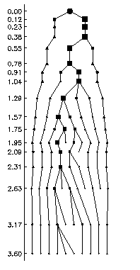
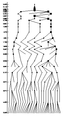
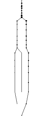
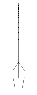
Figure 3.3: Left: Family tree of the cD galaxy of cluster A in the low-resolution simulation (see Table 3.1). Right: Family trees of the cD galaxy, the third-most massive galaxy, and a lower-mass galaxy in the high-resolution re-simulation of the same cluster. – The size of symbols is proportional to the logarithm of the mass of the galaxies at the corresponding redshift. Shown on the vertical axis on the left are the output redshifts used to reconstruct the family trees; these are different in both simulations. A galaxy in these trees is considered a progenitor of another galaxy if at least 50% of its stars are bound to its daughter galaxy, according to the SKID algorithm. Many more galaxies can be identified in the high-resolution simulation at similar redshift. The cD family tree is characterised by one dominant branch with a number of other branches merging into it, at both resolutions. Squares and triangles represent our classification of “merging” and “stripping” events, see Section 3.4.6. Circles correspond to redshift at which the galaxy is not releasing stars to the DSC.

We then build the family trees for all galaxies found at $z=0$ in all the 117 clusters of our sample. Given the adopted mass threshold of 32 star particle per galaxy, this amounts to an overall number of 1816 galaxies at redshift $z=0$, and 71648 galaxies in all redshift outputs.

Figure 3.3 shows the family tree of the cD galaxy of a cluster having virial mass $M{\rm vir}=1.6\times 10^{14}h^{-1}M_{\odot}$ (cluster A in Table 3.1). The cD galaxy family tree is complex and resembles a typical DM halo merger tree, with the cD being the result of a number of mergers between pre–existing galaxies. Other galaxies have a much simpler formation history, with fewer or no mergers of luminous objects. This is illustrated in the right part of Fig. 3.3 which shows merger trees from the high-resolution re-simulation of the same cluster, for the cD galaxy, the third-most massive galaxy in the cluster, and a low-mass galaxy. In more massive clusters, galaxies whose family trees are intermediate between that of the cD and the third-most massive galaxy can also be found. They are however among the most massive galaxies in their cluster, and they are often the most massive galaxy of an infalling subcluster, which has not merged completely with the main cluster yet.

Once the family trees of all galaxies in our clusters at $z=0$ are built, we then analyse the formation history of the DSC.

3.4.2 The epoch of formation of the DSC

Figure 3.4: Fraction of star particles found in the DSC at redshift $z=0$ which are already in the diffuse component at redshift $z$, for all clusters in our set. The inset show the same curves in logarithmic coordinates.

As already discussed, the star formation model used in our simulations implies that stars can only form inside existing gravitational potential wells, so that all DSC stars must have become unbound from their parent galaxies sometime after their formation. In Fig. 3.4, we plot the fraction of star particles in the DSC at $z=0$ which are already in the DSC at redshift $z$. The bulk of the DSC is created after $z\approx 1$, when on average only $\approx 30$ per cent of $z=0$ DSC star particles already reside outside their parent galaxies, with significant cluster-to-cluster variations. However, from the inset of Fig. 3.4 we note that the production of the DSC follows a power-law, thus implying that it is a cumulative process which, on average, does not have a preferred time scale. Willman et al. 2004 found a similar result based on the analysis of their high–resolution simulation of a single cluster, with a continuous growth of the DSC fraction and no preferred epoch of formation.

No statistically significant correlation is found between the fraction of DSC at $z=0$ and a number of possible tracers of the dynamical history of the cluster, such as the concentration of the NFW profile, the number of (DM–halo) major mergers, or the epoch of the last major merger. This suggests that the process of formation of the DSC is more related to the local dynamics of the interactions between galaxies and the group/cluster environment, rather than to the global dynamical history of the cluster.

3.4.3 DSC and the history of galaxies

We now proceed to establish which galaxies are the main contributors to the formation of the DSC. For each DSC star particle at $z=0$, we look for a $G_{j}$ galaxy at $z_{i}$ to which it last belonged. When this galaxy is found, we check whether the galaxy $G_{j}$ is associated with the family tree of a galaxy $G_{k}$ at $z=0$. If so, then the DSC star particle is associated with the “family tree” of the galaxy $G_{k}$. If the $G_{j}$ galaxy at $z_{j}$ is not associated with the family tree of any $G_{k}$ galaxies at $z=0$, but its family tree ends at $z_{j+m}$, then the DSC star particle is associated with a dissolved galaxy. If no bound structure is found, then the particle is associated with a volatile structure, and it is not considered in the subsequent analysis.

As a next step, we compute what fraction of the DSC particles comes from the family trees of galaxies at $z=0$, as a function of the binned galaxy mass at $z=0$, $M_{\rm gal}(z=0)$. Then the DSC mass $M^{*}_{\rm DSC}(M_{\rm gal})$ obtained for each $M_{\rm gal}(z=0)$ bin is normalised by the total stellar mass of the respective cluster. The total fraction $F_{\rm DSC}$ for each cluster is finally given by the sum over all contributions from all galaxy masses at $z=0$.

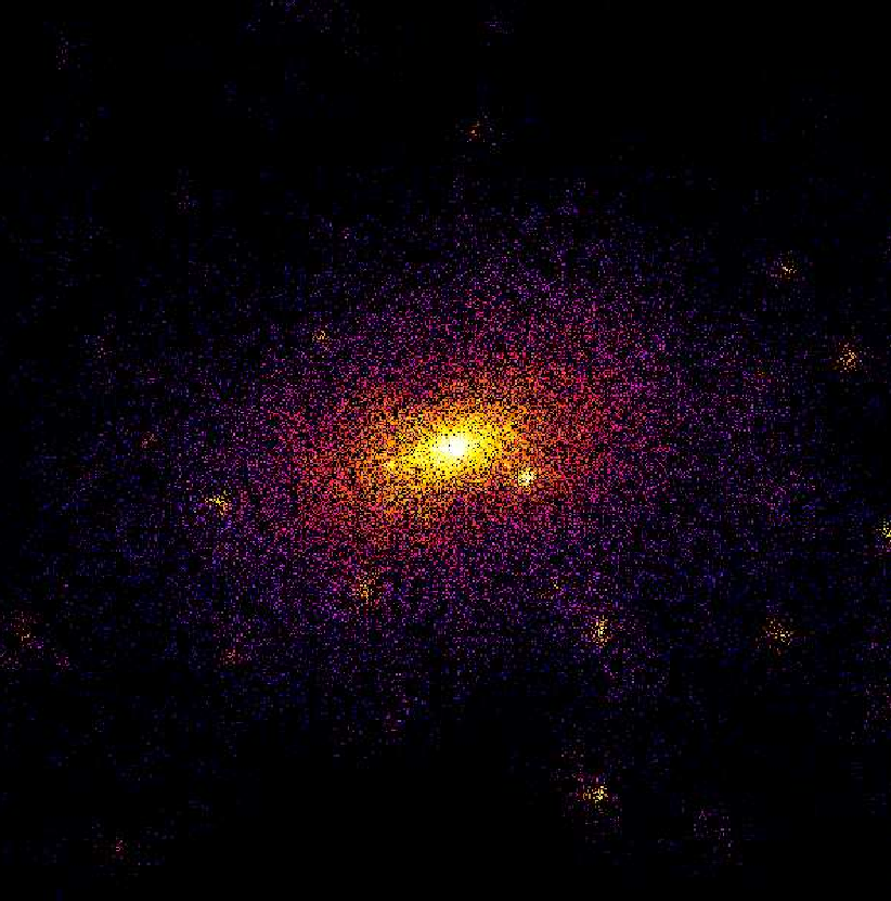
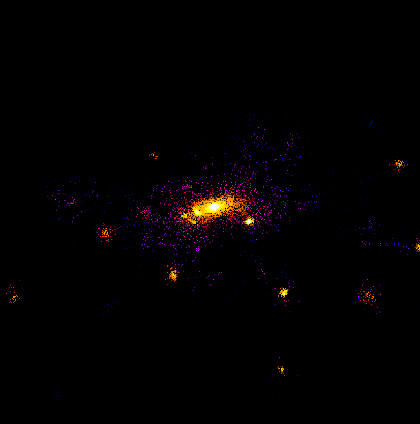
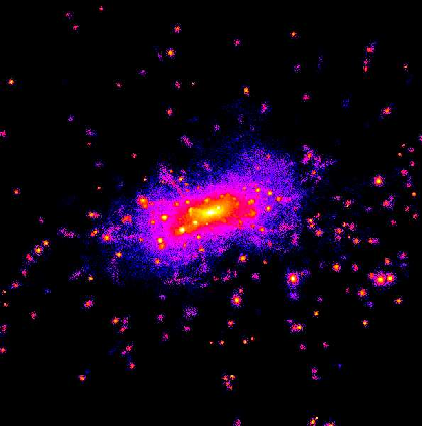
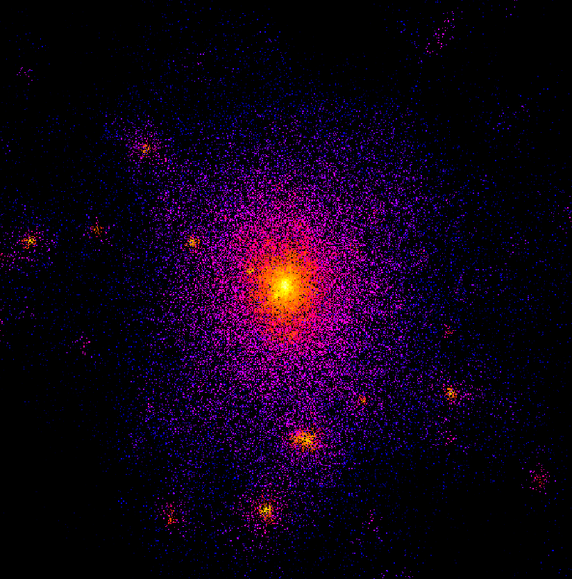
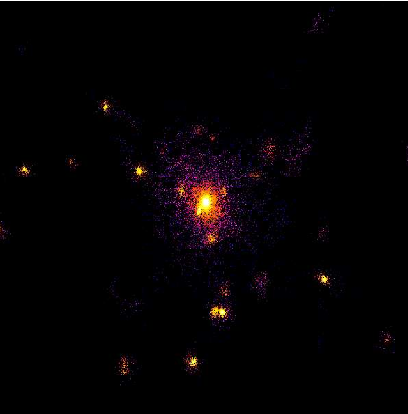
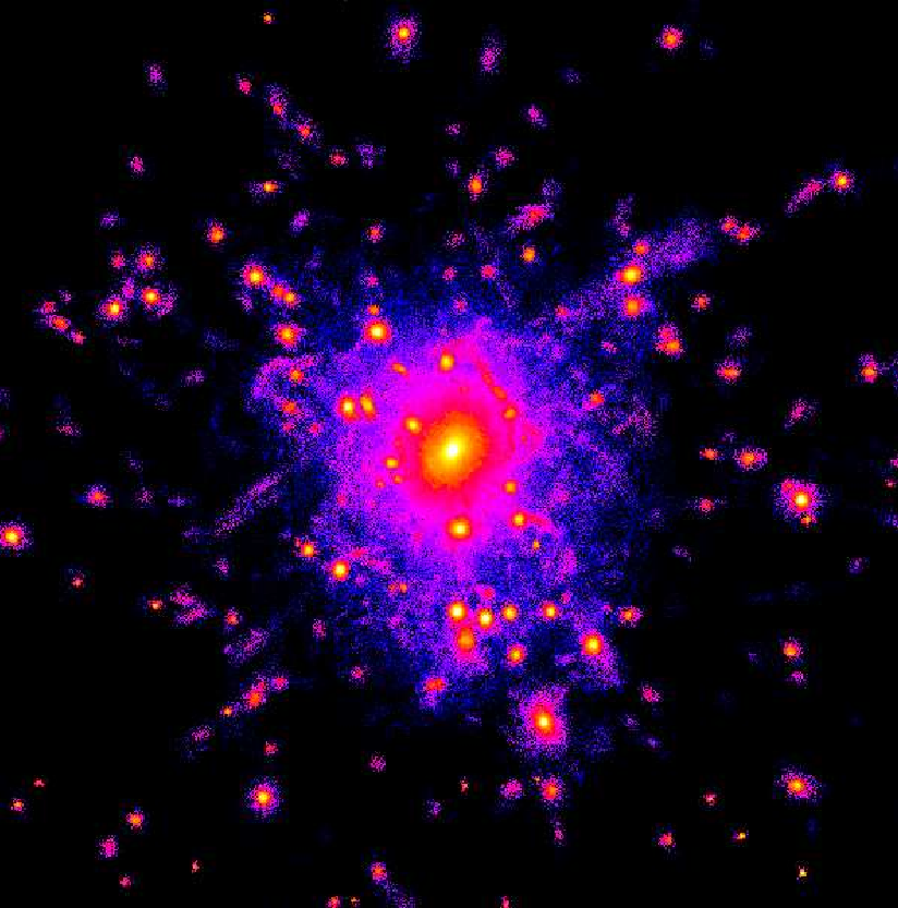
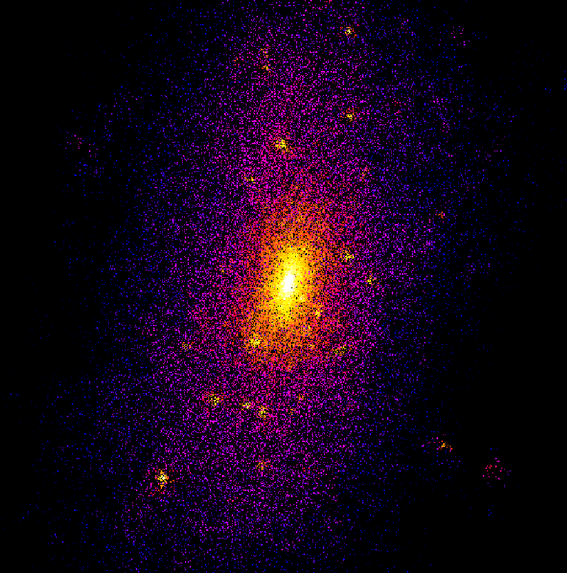
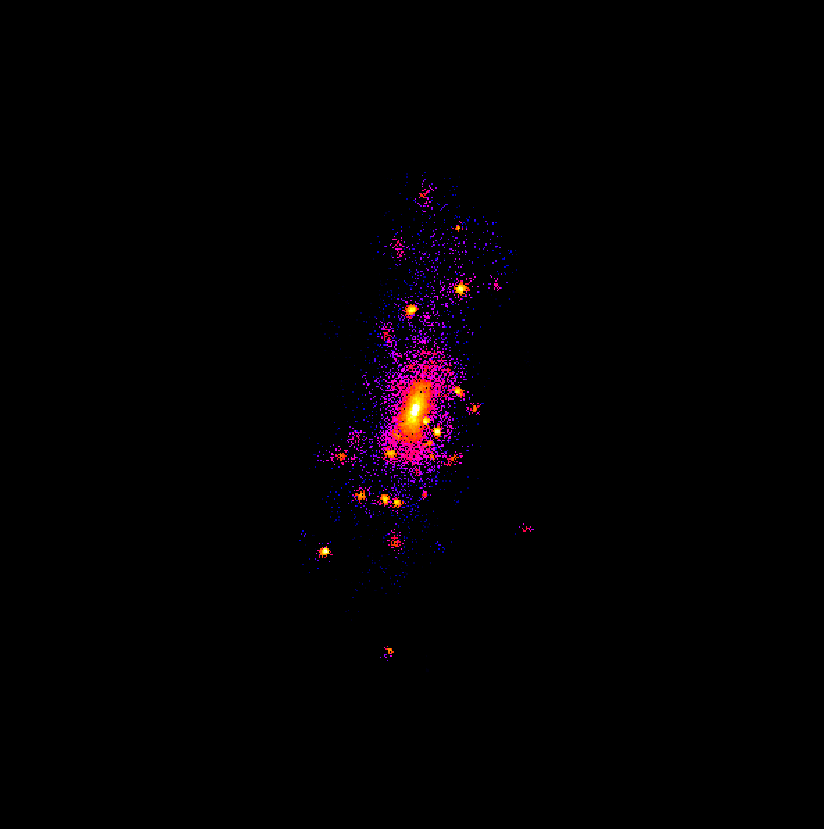
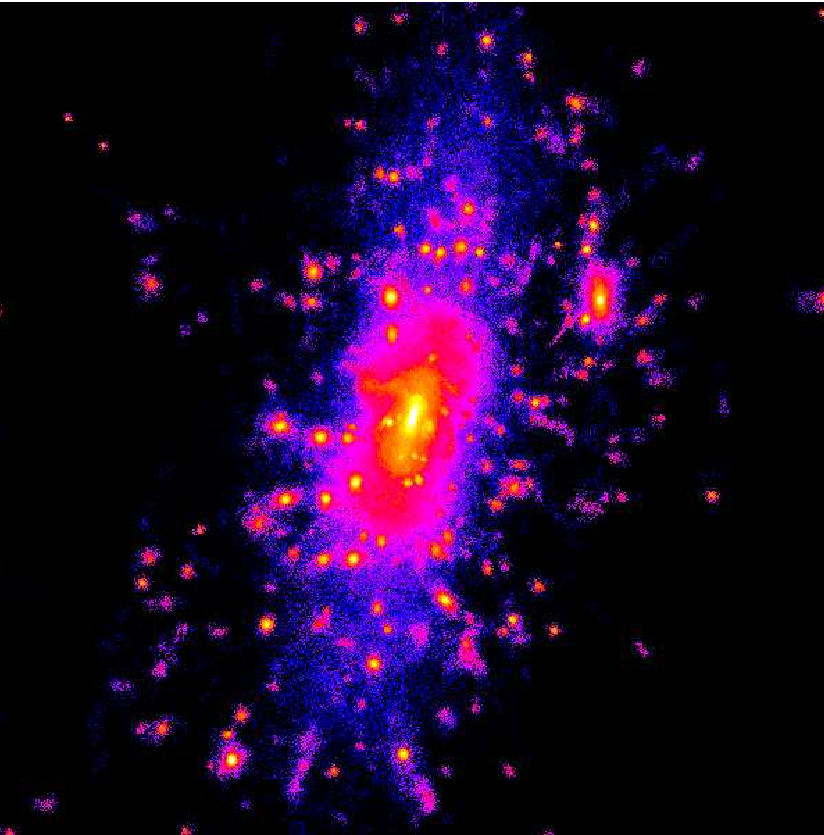
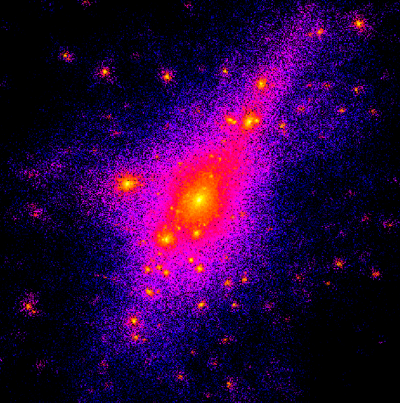
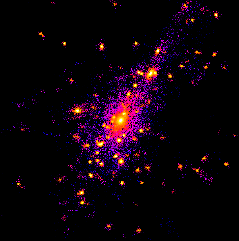
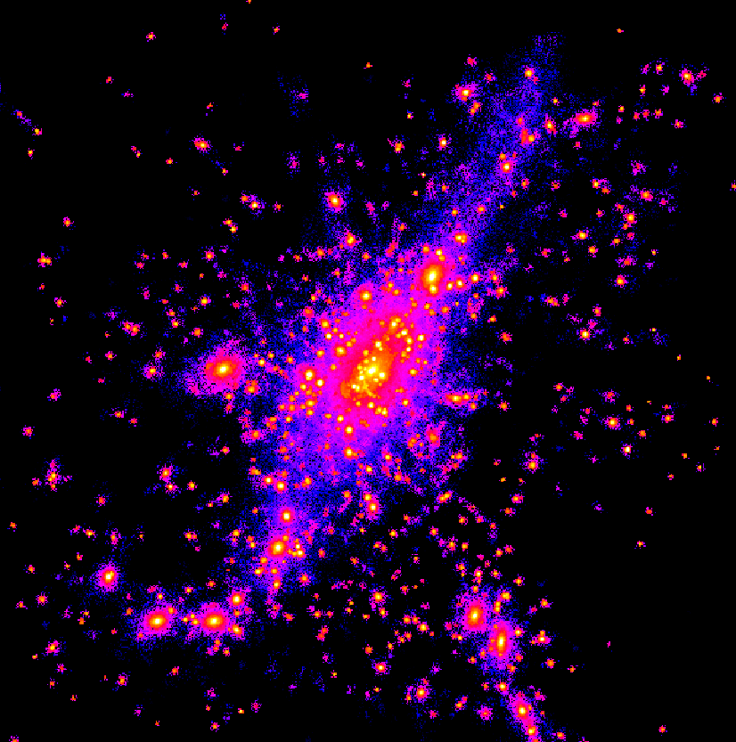
Figure 3.5: The distribution of the dark matter (left panels) and of the stars (canter panels) for clusters (A), (B), (C), (D) from the cosmological simulation, and the distribution of stars in the high-resolution re-simulations of the same four clusters (right panels), all at redshift $z=0$. The frames are $3h^{-1}$ Mpc on a side in the first three rows and $6h^{-1}$ Mpc in the last row, corresponding to $\approx 2R_{\rm vir}$ for the four clusters (see Table  3.1). They show density maps generated with the SMOOTH algorithm, applied separately to the DM and star particle distributions. Colour scale is logarithmic and different for DM and stars: from $10^{-0.5}$ to $10^{5}$ times critical density and from $10$ to $10^{6}$ times critical density for stars and DM particles, respectively.

3.4.4 Standard resolution simulation - 4 exemplary clusters

We discuss the results of this analysis for the four clusters shown in Figure 3.5. The figure shows the density distribution of DM and star particles in the four clusters, and also the distribution of star particles in the high-resolution re-simulation of these clusters. The main characteristics of these clusters are given in Table 3.1. The galaxies identified by SKID correspond to the densest regions plotted in yellow in this Figure.

These four clusters cover a wide range of masses (see Table 3.1), and the two intermediate mass clusters B and C have very different dynamical histories: cluster B experienced a major merger at $z\approx 1$, while cluster C is undergoing a merger event at $z=0$ which began at $z\approx 0.2$.

Figure 3.6: Histograms of the fraction of DSC star particles identified at $z=0$, associated with the family trees of $z=0$ galaxies of different masses: $F_{\rm DSC}(M_{\rm gal})=M^{*}_{\rm DSC}(M_{\rm gal})/M^{*}_{\rm tot}$. Results are reported for the four clusters shown in Figure 3.5 (see also Table 3.1). We use 10 galaxy mass bins, logarithmically spaced, from $M_{\rm min}=1.1\times 10^{10}h^{-1}M_{\odot}$ to $M_{\rm max}=3.1\times 10^{12}h^{-1}M_{\odot}$. The leftmost column in each panel gives the contribution from dissolved galaxies, regardless of their mass. It is the mass range only for sake of clarity. For these 4 clusters, the only family tree contributing to the rightmost column is that associated with the BCG.

Figure 3.7: Histograms of the relative contribution to the DSC from the formation history of galaxies belonging to 10 $M_{\rm gal}(z=0)$ mass bins, for the entire set of clusters in the simulation, and as a function of cluster mass. Upper left panel: average over the whole 117 cluster set. Upper right panel: average over the 71 least massive clusters. Lower right panel: average over the 11 most massive clusters. Lower left panel: average over the 35 intermediate–mass clusters. We use 10 $M_{\rm gal}(z=0)$ mass bins, logarithmically spaced from $M_{\rm min}=1.1\times 10^{10}h^{-1}M_{\odot}$ to $M_{\rm max}=3.1\times 10^{12}h^{-1}M_{\odot}$. The leftmost column in each panel represents the contribution from dissolved galaxies, regardless of their mass. The rightmost column in each panel shows the contribution from the history of the single most massive galaxy of each cluster, regardless of its actual mass.

In Fig. 3.6, the histograms show the mass fractions of the DSC associated with the family trees of $M_{\rm gal}(z=0)$ galaxy for these four clusters. From Fig. 3.6, we can draw the following picture for the origin of the DSC:

• The bulk of the DSC comes from the formation history of the most massive galaxy, except in the most massive cluster D;

• Dissolved galaxies give a significant contribution in two out of the four clusters (clusters B,D);

• All other galaxy family trees provide either a small (clusters A–C) or modest (cluster D) contribution to the DSC.

Label	$M_{\rm vir}$	$R_{\rm vir}$	$F_{\rm DSC}^{\rm all}$	$F_{\rm DSC}$	$F_{\rm DSC}^{\rm vol}$	$F_{\rm DSC}^{\rm dis}$	$F_{\rm DSC}^{\rm ng}$
	[$10^{14}h^{-1}M_{\odot}$]	[$h^{-1}$ kpc]
A	1.6	1200	0.33	0.20	0.11	0.02	0.02
B	2.5	1290	0.36	0.21	0.12	0.10	0.05
C	2.9	1350	0.45	0.27	0.14	0.04	0.04
D	13.0	2250	0.45	0.22	0.23	0.06	0.00
Ave	–	–	0.34	0.18	0.09	0.04	0.07

Table 3.1: Virial masses, viral radii, and DSC fractions for the four clusters A–D shown in Fig. 3.5. The fraction shown in the column 4, $F_{\rm DSC}^{\rm all}$, includes the contribution from low-density galaxies. The $F_{\rm DSC}$ value in column 5 is obtained omitting the particles unbound from low-density galaxies. For completeness we report the fraction $F_{\rm DSC}^{\rm vol}$ of discarded particles from low-density or volatile structures in column 6; the fraction $F_{\rm DSC}^{\rm dis}$ of star particles from dissolved galaxies in column 7, which corresponds to the leftmost columns in the histograms of Figs. 3.6 and 3.7; the fraction $F_{\rm DSC}^{\rm ng}$ of star particles that never belonged to any galaxy in column 8. The last row of the table reports the average DSC fractions for the whole sample of 117 clusters.

In the case of the most massive D cluster, a significant contribution to the DSC comes from intermediate–mass galaxies. Willman et al. 2004 also found in their simulation of one cluster with mass similar to our cluster D, that galaxies of all masses contributed to the production of the DSC. Our results suggest that when the cluster statistics is enlarged, such cases are rare; in our set this is the case in 3 clusters out of the 11 most massive ones from the whole set of 117 clusters.

Furthermore, Figure 3.5 shows that cluster D is still dynamically young, with a number of massive substructures both in the DM and in the star particle distribution. This is probably the main reason why the DSC formation in this cluster is not dominated by the most massive galaxy: the sub–clumps contain galaxies of various masses which experienced several mergers in their history, producing a significant amount of DSC. This is also confirmed by the analysis of the family trees of the galaxies belonging to this cluster: 12 of the 85 identified galaxies had more than one merger in their history, while usually only one or two galaxies in each cluster are found to have a complex family tree.

In the other 3 clusters, the largest fraction of the DSC star particles is associated with the formation history of the cluster’s most massive galaxy. Cluster B also shows a large contribution coming from dissolved galaxies: perhaps this suggests that the tidal field associated in this cluster was more efficient in disrupting galaxies rather than stripping some of their stars.

Our analysis so far does not exclude that some fraction of the DSC at $z=0$ is produced in subclusters or groups, such as suggested by Rudick et al. 2006. In fact, the analysis of cluster D suggests that this does happen. If these sub-clusters or groups migrate to the centre of the cluster and finally merge, our procedure would associate the DSC particles unbound from these structures with the family tree of the cD at $z=0$.

However, if tidal stripping of the least–bound stars in all galaxies were the main mechanism for the production of the DSC, we would expect a more similar fraction of DSC star particles from all galaxy masses.

3.4.5 Standard resolution simulation - statistics for 117 clusters

We now turn to the statistical results for the whole set of 117 clusters. In Figure 3.7 we show the contributions from the same galaxy mass bins as before, but averaged over all clusters and over different cluster mass ranges. To obtain our average values, we sum the mass of diffuse star particles in all clusters in the appropriate galaxy mass bin and normalise it to the total stellar mass of all clusters. This procedure creates a “stacked-averaged” cluster. The average value of the diffuse light fraction is $<F_{\rm DSC}>=16\%$ of the total stellar mass.

In the upper left panel of Fig. 3.7, showing the fractional contributions from galaxy mass bins averaged over the whole cluster set, the rightmost column represents the contribution from the clusters’ BCGs only. The value of the mass for this class is arbitrary; this bin has been plotted separately since the masses of the BCGs increase with cluster mass and, therefore, BCGs in different clusters can belong to different mass bins. This effect is clearly visible in the upper right panel of Fig. 3.7, which refers to the less massive clusters in our set. For these clusters, the BCGs fall into two mass bins, with the majority of them falling in the second most massive bin.

The other three panels of Fig. 3.7 show the same relative contributions when the average is performed over (i) the 11 most massive clusters (lower right panel, $M_{\rm vir}>4\times 10^{14}h^{-1}M_{\odot}$ with $<F_{\rm DSC}>=19\%$), (ii) the 35 clusters having intermediate mass (lower left panel, $2\times 10^{14}<M_{\rm vir}<10^{14}h^{-1}M_{\odot}$ with $<F_{\rm DSC}>=18\%$), and (iii) the 71 least massive clusters (upper right panel, $M_{\rm vir}<2\times 10^{14}h^{-1}M_{\odot}$ with $<F_{\rm DSC}>=13\%$). These average values show a weak trend with cluster mass in the production of the DSC. As a further test, we have divided clusters according the amount of the DSC fraction itself. This analysis also confirms that the dominant contribution to the DSC comes from the BCG family tree, independent of $F_{\rm DSC}$ as expected, given the weak relation between $F_{\rm DSC}$ and cluster mass. We also find that the contribution from dissolved galaxies is slightly higher for clusters with $<F_{\rm DSC}>$ greater than $25\%$.

The results shown in Fig. 3.7 are consistent with the previous analysis of the four clusters: the bulk of the DSC is associated with the galaxies in the family tree of the most massive galaxy of each cluster. Galaxies in the family trees of smaller $z=0$ mass bins contribute only few tenths of the fraction from the BCG family tree.

Dissolved galaxies also contribute significantly to the DSC, but it is possible that their estimated contributions are affected by some numerical effects. In fact, if the analysis is restricted to galaxies whose density is within $1\sigma$ of the observed galaxy density estimate (Section 3.2), then the contribution to the $F_{\rm DSC}$ from the BCG rises to $\approx 76\%$, while that from dissolved galaxies drops to $\approx 8\%$. As expected, most “dissolved galaxies” are those with low densities, which indicates that their contribution to the DSC may be affected by the limits in numerical resolution. This needs further work to be properly understood.

3.4.6 Merging and stripping in galaxy family trees

Figure 3.8: The fraction of DSC stars arising in the “merger” part, $F_{\rm DSC}^{\rm mrg}/F_{\rm DSC}$, and in the “stripping” part, $F_{\rm DSC}^{\rm strp}/F_{\rm DSC}$, of the galaxy family trees, as a function of their $z=0$ galaxy mass class (solid and dashed lines, respectively). The asterisks mark the values for the contribution from the BCG family tree only. See text for details.

As shown in Fig. 3.3, the BCG is the galaxy that experiences the largest number of luminous mergers during its assembly, and it often has the most complex family tree in a cluster. Our result that a large fraction of DSC is associated with the BCG supports a scenario where mergers release stars from their parent galaxies to the intracluster space.

To investigate this further, we estimate the fraction of DSC particles associated with the merger part of the family trees, and with the stripping part of the family trees, as follows. We define a DSC star particle to arise from a merger at redshift $z_{j}$ if the galaxy it was last bound to has more than one progenitor at $z_{j-1}$. The DSC particles coming from the progenitors at $z_{j-1}$ are also defined as arising from a merger. We take a DSC star particle to be unbound through stripping if the galaxy it was last bound to at redshift $z_{j}$ has only one progenitor at $z_{j-1}$. The different parts of the family trees are indicated in Fig. 3.3, where the squares represent the merger part of the tree, triangles the stripping part, while circles mark the part of the tree where no stars are released to the DSC.

In Fig. 3.8, we show the fraction of the DSC star particles which arise from the merger part of the family tree, as a function of the final galaxy mass. For high–mass galaxies, most of the DSC originates from the merger part of their family trees. Low mass galaxies, on the other hand, lose stars only via stripping. After each merger between massive galaxy progenitors, up to $30\%$ of the stellar mass in the galaxies involved has become unbound. This large fraction perhaps indicates that many of these mergers take place either in strong tidal fields generated by the mass distribution on larger scales, or just before the merger remnants fall into their respective cluster.

Combined with the result that most of the DSC star particles are associated with the family trees of the most massive galaxies, the fact that most of the DSC is released during merger events implies that the bulk of the DSC originates in the merger assembly of the most massive galaxies in a cluster. The more standard picture for the formation of the DSC, in which all galaxies lose their outer stars while orbiting in a nearly constant cluster gravitational potential, is not confirmed by current cosmological hydrodynamic simulations. It appears that strong gravitational processes, linked to the formation of the most massive galaxies in the cluster and to mergers between luminous objects, are the main cause for the creation of the DSC.

A further mechanism possibly at work is the complete disruption of galaxies, which also takes place preferentially in the cluster central regions. In our cosmological simulation this formation mechanism for the DSC is likely to be enhanced by numerical effects, which tend to produce under-dense galaxies. We address this issue below when we discuss our high-resolution simulations of the clusters in Fig. 3.5.

3.4.7 cD Halo vs Intracluster Light

So far, we have made no attempt to distinguish between a component of DSC associated with the unbound halos of the central cD galaxies, and a more cluster-wide DSC. Our definition of the DSC includes stars in the cluster central regions and a part of these may well be in the form of cD halos (see the Appendix). Independent of how well a distinction between these two components can be made, one might expect that the fraction of DSC stars that comes from the merging tree of the BCG would be most concentrated towards the cluster centre. To shed some light on this question, we show in Fig. 3.9 the same analysis for the average over all galaxy clusters in the simulation as in Fig. 3.7, but now excluding all DSC particles residing in the central $250h^{-1}$ kpc around their cluster centres. The remaining total DSC fraction drops to about $6\%$, less than half of the total, reflecting the steep radial profile of the DSC (Murante et al. 2004, Zibetti et al. 2005. For $R>250h^{-1}$kpc, the family trees of the most massive galaxies still provide the largest contribution to the DSC (per mass bin), but the cumulative contributions from family trees of less massive galaxies now dominates the BCG component by a factor $\sim 2$. At the same time, the relative contribution from dissolved galaxies increases. The lower panel of Fig. 3.9 shows the same analysis but now excluding DSC particles within $0.5R_{\rm vir}$. In this case, the $<F_{\rm DSC}>$ drops to $\sim 1\%$, with the fraction from the BCG family tree now similar to that from other galaxies.

Since the BCG halo is likely to be less extended than $250h^{-1}$ kpc, our interpretation of the results in Fig. 3.9 is that the merger part of the most massive galaxy family tree in each cluster contributes substantially to the DSC also outside the cD halo. However, at radii $250h^{-1}\mbox{kpc}<R<0.5R_{\rm vir}$, the cumulative contribution from the family trees of other massive galaxies dominates the DSC. Presumably, these are the most massive galaxies within subgroups, which fell into the cluster and brought in their own DSC, but which have not yet had time to merge with the BCG. This interpretation is consistent with the simulation results of Willman et al. 2004, Rudick et al. 2006. Only in the outskirts of clusters, at $R>0.5R_{\rm vir}$, we find that the DSC particles come preferentially from the stripping part of family trees from all galaxy mass bins.

The relevance of merger events for the formation of the DSC may explain why diffuse light is more centrally concentrated than galaxies, in both observations (Zibetti et al. 2005, Arnaboldi et al. 2002) and in simulations (M04, Willman et al. 2004, Sommer-Larsen et al. 2005). Stars from accreted satellite galaxies form extended luminous halos around massive galaxies (Abadi et al. 2006), and if these massive galaxies end up concentrated to the cluster centre, their diffuse outer envelopes would preferentially contribute to the DSC in the cluster centre.

Our results on the origin of the DSC are also consistent with the predictions by D’Onghia et al. 2005 that simulated fossil galaxy groups have a larger amount of intra–group stars than normal groups. Indeed, if fossil groups are the dynamically most evolved groups, then their galaxies had more time to interact and build up the central elliptical galaxy ( see e.g. D’Onghia et al. 2005). The number of galaxy–galaxy mergers in groups appears to be closely related to the amount of DSC liberated (Sommer-Larsen 2006). A direct comparison of our results with Willman et al. 2004 is difficult because of their re-normalisation of the simulated galaxy luminosities in order to fit the observed luminosity function, but these authors also concluded that luminous galaxies provide a substantial contribution to the DSC.

Figure 3.9: The same as in Fig. 3.6, averaging over all clusters, but excluding the DSC star particles inside $R=250h^{-1}$ kpc (upper panel) and inside $0.5R_{\rm vir}$ of each cluster (lower panel).

3.5 High resolution simulations and the effects of numerical resolution on the formation of the DSC

To address the stability of our results against mass and force resolution, we have re-simulated three clusters extracted from the cosmological box (A,B,C from Table 3.1) with 45 times better mass resolution and $\simeq 3.6$ times smaller gravitational softening. A detailed presentation of these re-simulations is given in Borgani et al. (2006). Galaxies formed in these high-resolution simulated clusters have densities similar to those shown in Fig. 3.1 for masses larger than $\approx 10^{11}h^{-1}M_{\odot}$, and the low–density tail seen in Fig. 3.1 is shifted towards lower masses, in accordance with the better resolution.

We carry out our study of the DSC in these three clusters following the procedure described previously, discarding DSC star particles contributed from under-dense and volatile structures. In Fig. 3.10, we show the fractions of DSC star particles identified at $z=0$ and originating from the history of galaxies belonging to different mass bins. The full columns refer to the analysis of the high–resolution simulations of the three clusters, while the open columns show the results from Fig. 3.7 for the low-resolution simulations.

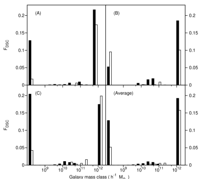
Figure 3.10: Histograms of the fraction of the $z=0$ DSC particles associated with galaxy family trees in 15 $M_{\rm gal},(z=0)$ mass bins, for the three clusters re–simulated at high–resolution (filled columns), and in the standard–resolution (empty columns, cf. Fig. 3.6). The mass bins are logarithmically spaced, from $M_{\rm min}=2\times 10^{8}h^{-1}M_{\odot}$ to $M_{\rm max}=3.1\times 10^{12}h^{-1}M_{\odot}$. The leftmost columns show the contribution from dissolved galaxies, regardless of their mass. Upper-left, upper-right and lower-left panels show the comparison for clusters (A), (B), (C), respectively; the lower-right panel show the average for these three clusters.

In the clusters simulated with high resolution, the results on the origin of the DSC are consistent with what we found for the standard resolution. The DSC builds up in parallel with the formation of the most massive galaxies in the cluster. The amount of DSC star particles produced during the history of all other galaxies is still negligible when compared with the contribution from the most massive cluster members. With the increase in resolution, more DSC stars now come from dissolved galaxies in clusters A and C, and an increasing number comes from the family tree of the cD in clusters A and B.

Another question is whether the results on the DSC are affected by the efficiency of the kinetic feedback from SNe. To address this point, we re-simulate cluster A at the resolution of the cosmological box, with (i) the same feedback efficiency and (ii) the speed of the galactic ejecta set to zero. We find very similar results in the strong and weak feedback cases: no significant contribution from intermediate mass galaxies, 7.5% and 8.7% of the DSC coming from dissolved galaxies, and 89.7% and 87.1% of the DSC originating from the history of the BCG, respectively.

However, the overall fraction of intracluster stars in these three clusters changes between our low-resolution and high-resolution simulations. Once the star particles from volatile and under-dense galaxies are discarded, the fraction of DSC within the virial radius of clusters A, B and C is $F_{\rm DSC}=0.37,0.28,0.41$ in the high resolution simulations, compared with $F_{\rm DSC}=0.20,0.21,0.27$ in the standard resolution case. The overall increase of the DSC fraction at high-resolution is mostly, but not only, related to an increase in the fraction of DSC from dissolved lower-mass galaxies (see Fig. 3.10).

This result is not in contradiction with Sommer-Larsen 2006 finding that the DSC fraction in his simulations remains constant when the resolution is increased. This is because in the Sommer-Larsen 2006 simulations the numerical resolution is increased without adding the corresponding higher frequencies in the initial power spectrum. Then the number of low-mass galaxies and (small–object) mergers does not increase significantly, and one expects an approximately constant DSC fraction. This suggests that the increase in the DSC fraction in our high-resolution simulations is related to the addition of small objects through the added high-frequency part of the power spectrum.

We expect that the effect of numerical overmerging is reduced at higher resolution (e.g. Borgani et al. 2006 and references therein for a full discussion of this issue), so we must look for other effects that could dominate the disruption of the smaller galaxies. The results from Sommer-Larsen 2006 also rule out a significant effect from stronger tidal shocks during high-speed collisions with low-impact parameters, when galaxies become denser at higher numerical resolution. One possibility is that, when the resolution is increased, the number of numerically resolved mergers increases. On the basis of the results reported above, this could turn into an increased efficiency in the production of the DSC. If so, a solution to the problem could lie in a more realistic feedback mechanism.

Another issue related to the numerical resolution concerns the number of small ($\lg 10^{11}h^{-1}M_{\odot}$) galaxies identified in these simulations. Recent determinations of the K–band luminosity function for galaxies in clusters give a faint–end slope between $\alpha=-0.84$ and $\alpha=-1.1$ Lin & Mohr 2004. The faint end slope of the stellar mass function in our cosmological simulation is flatter than the observed luminosity function: we obtain $\alpha\approx-0.7$, thus implying that we miss a number of small galaxies. A shallower slope of the faint end of the luminosity function is a general problem of numerical simulations like those presented here ( e.g. Willman et al. 2004).

If the number of low–mass galaxies is underestimated in the simulations, then their contribution to the DSC would be affected in the same way. To estimate this effect, we computed how many galaxies we would expect in each mass bin of Fig. 3.7, if the faint end of the stellar mass function was given by $n(M)=K\cdot(M/M_{*})^{\alpha}$, with $\alpha=-0.84$,$-1.1$ and $M_{*}=5\cdot 10^{11}h^{-1}M_{\odot}$. The constant is fixed by requiring that the number of galaxies for a mass $M=2\cdot 10^{11}h^{-1}M_{\odot}$ is the same as in the simulation. This method is similar to the re-normalisation of the luminosity function in Willman et al. 2004. We then assume that the missed galaxies contribute the same relative fraction of their mass to the DSC as the present-day galaxies of similar mass in the simulation, and multiply the fraction $F_{\rm DSC}(M)$ by the ratio of $N(M)/N_{s}(M)$, where $N_{s}(M)$ is the number of simulated galaxies found in the bin and $N(M)$ is the integral of $n(M)$ in the same bin. This correction is applied to each mass bin up to $2\cdot 10^{11}h^{-1}M_{\odot}$. Fig. 3.11 shows the result of this correction when it is applied to the average distribution of $F_{\rm DSC}$ for the whole set of three clusters (lower right panel of Fig. 3.10). The DSC production is still dominated by the contribution coming from the BCGs in the clusters. The effect of such correction is to bring the contribution of the mass bins corresponding to masses $M<10^{11}h^{-1}M_{\odot}$ to the same levels of the others. Correction is stronger for the smaller mass bins. Nevertheless, the contribution of these mass classes to the global $F_{\rm DSC}$ remain small. Note that the increases in $F_{\rm DSC}(M)$ values in the mass bin $\sim 2\cdot 10^{11}h^{-1}M_{\odot}$ is due to a few galaxies with mass $1.5<M<2\cdot 10^{11}h^{-1}M_{\odot}$, whose contribution to the DSC has been corrected. The contribution $F_{\rm DSC}(M)$ from galaxy having masses smaller than $\approx 1.1\cdot 10^{10}h^{-1}M_{\odot}$ in the three re-simulated clusters, where they are resolved, is very small.

A further issue to be considered is that all galaxies are spheroidal at the numerical resolution of these cosmological simulations; indeed, the self–consistent formation of disk galaxies is still a challenge in hydrodynamic $\Lambda$CDM simulations. Are our conclusions on the origin of the DSC likely to be affected by the absence of disk galaxies in our cosmological simulation? Generally, disk galaxies are more vulnerable to tidal forces, but the amount of matter lost in tidal tails is small, unless the tidal field is very strong, whereas elliptical galaxies lose their outer stars more easily. We do not expect that it would make a lot of difference for the amount of DSC released in the merging processes leading to the formation of the cluster BCG galaxies and most of the DSC, if a fraction of the participating galaxies were disk galaxies. However, this needs to be checked once simulations can reproduce disk galaxies. Independent arguments based on tidal stripping from disk galaxies in a semi–analytical model of galaxy formation (Monaco et al. 2006, Monaco et al. 2006) suggest that at most $\sim 10$ per cent of the total stellar mass of each cluster is contributed to the DSC by the “ quiet tidal stripping” mechanism, even for the most massive clusters where observations points toward a larger amount of diffuse stars.

As already discussed in Section 3.2, our force resolution is not enough to resolve the inner structure of the simulated galaxies. As a consequence, their internal density is likely to be underestimated, so that these galaxies are more vulnerable to tidal stripping and disruption than real galaxies. This numerical artifact is not completely removed even in our high resolution re-simulations, where the Plummer–equivalent softening is $\simeq 2h^{-1}$ kpc. Even when simulated galaxies with central densities lower than a chosen threshold are removed, we still find that less massive galaxies are less dense than massive galaxies, at variance with observational results. This probably accounts for most of the contribution to the DSC from dissolved galaxies. If we had more realistic, denser small galaxies in the simulation, this might decrease their contribution to the DSC even more.

We can summarise the discussion of systematics effects in our analysis related to numerical resolution as follows:

1. Our conclusion, that the formation of the DSC is intimately connected with the build–up of the cluster’s BCG, is confirmed in higher numerical resolution simulations;

2. this conclusion appears insensitive to the limitations of current simulations in reproducing low-mass galaxies, disk galaxies, and the faint-end luminosity function;

3. resolving galaxies with smaller masses in the high-resolution simulations does not have a strong effect on the formation and evolution of the DSC;

4. the global value of $F_{\rm DSC}$ depends on resolution, and it increases in simulated clusters with higher resolution. The value of this fraction has not converged yet, in the range of numerical resolution we examined.

Figure 3.11: Corrections to $F_{\rm DSC}$ to account for the low–mass end of the galaxy mass function. The solid line is the uncorrected $F_{\rm DSC}$; the dashed and the dotted lines give the corrected value when the low–mass end of the galaxy cluster stellar mass function has a slope $\alpha=-0.84$ and $\alpha=-1.1$, respectively.

3.6 How do stars become unbound? On the origin of the diffuse stellar component

In cosmological hydrodynamic simulations, stars form in galaxies. The DSC is built up from stars that are dissolved from their parent galaxies. This is an ongoing process linked to the accretion of substructure (see above and also Willman et al. 2004); in fact, most of the DSC originates at relatively recent redshifts. Stars may be added to the DSC through a number of dynamical processes, listed here in the approximate time sequence expected during the infall of a significant subcluster:

1. Tidal stripping of the preexisting diffuse stellar population from the in-falling subcluster or group: The DSC in the substructure, generated by dynamical processes in the substructure, is added to the DSC of the main cluster when both structures merge.

2. Stripping from extended galaxy halos created in substructures: In subclusters or galaxy groups, galaxy interactions occur with lower relative velocities and are thus generally more damaging than in interactions with the high relative velocities typical for galaxy clusters. Interactions or mergers within substructures may create loosely bound stellar halos which are stripped from their parent galaxies and the substructure when entering the cluster tidal field (Mihos et al. 2004, Rudick et al. 2006). This stripping may be delayed when the merging in the subcluster happens before its accretion, or immediate when the galaxy interactions occur already deep in the tidal field of the main cluster.

3. Tidal shocking and stripping during merger with the cD galaxy: The massive galaxies in the substructure generally interact with the cluster centre and the cD galaxy on near-radial orbits (see Figure 3.12). In a high-speed encounter of a massive galaxy with the cD, stars from both galaxies may gain sufficient energy to be (almost) tidally unbound from their parent galaxies. The tidally shocked stars from the intruder are then subsequently unbound by the ambient tidal field or further tidal shocks, remaining at similar orbital energies as their mother galaxy had at the time. Those from the cD galaxy become part of the cD envelope. The process may happen several times as the intruder galaxy orbit decays by dynamical friction. This mechanism is related to the cannibalism scenario for the growth of the cD galaxy, described in Ostriker & Hausman 1977, Merritt 1995 and others; however, here the dynamical friction appears to be more effective, presumably due to the large dark matter mass associated with the infalling substructure.

4. Tidal dissolution of low-density galaxies: These galaxies may enter high-density regions of the cluster along their orbits, such as the dark matter cluster centre, and dissolve completely if of sufficiently low density.

5. Tidal stripping in galaxy interactions: Stars may be torn out from galaxies during tidal interactions along their orbits in the cluster, and be dissolved from their parent galaxies by the cluster tidal field. The participating galaxies survive as such. Galaxies of all masses are affected. The last two processes together are often described as harassment (Moore et al. 1996).

The statistical results of the previous sections allow us to put some constraints on the relative importance of these various processes, and to identify further work needed to clarify the origin of the diffuse stellar population in galaxy clusters. These results can be summarised as follows.

• Most of the DSC is liberated from galaxies in the merger tree of the most massive, central galaxy in the cluster, i.e., simultaneously with the build-up of this galaxy.

• If only the fraction of the DSC outside $250{\rm kpc}$ from the cluster centre, i.e., outside the cluster dominant galaxy’s halo, is considered, the contribution from the BCG family tree is comparable to that from other massive galaxies. Only outside $\sim 0.5R_{\rm vir}$ do galaxies of all masses contribute to the DSC.

• There is a further, sizable contribution to the DSC in the simulations, from dissolved galaxies. However, the fraction of DSC stars from dissolved galaxies depends directly on the simulations’ ability to faithfully represent the lower mass galaxies, and is seen to vary strongly with the resolution of the simulation. This contribution to the DSC is thus currently uncertain; the prediction from the simulations is likely to overestimate the contribution of dissolved galaxies to the ICL in observed clusters.

• About 80% of the DSC that comes from the merger tree of the cD galaxy, is liberated shortly before, during, and shortly after major mergers of massive galaxies. About 20% is lost from these galaxies during quieter periods between mergers.

• In each significant merger, up to $30\%$ of the stellar mass in the galaxies involved becomes unbound.

• Most of the DSC is liberated at redshifts $z=0-1$.

These results imply that the main contribution to the DSC in our simulations comes from either tidal shocking and stripping during mergers with the cD galaxy in the final cluster (mechanism iii), and/or from merging in earlier subunits whose merger remnants later merge with the cD (i, ii). The traditional tidal stripping process (v) appears to contribute only a minor part of the DSC but may be the dominant process for the small fraction of the DSC that ends up at large cluster radii.

Further work is needed to see which of the channels (iii) or (i,ii) is the dominant one, and whether in the latter the contribution of the preexisting DSC in the accreted subclusters (i) dominates over that from extended galaxy halos (ii). The work of Willman et al. 2004 and Rudick et al. 2006 shows that the contribution from infalling groups is important but the division between the channels (i) and (ii) is not clear. In this case, our results imply (a) that merging must have been important in these groups, and (b) that the massive galaxies in the infalling groups that carry most of the final DSC will mostly have merged with the BCG by $z=0$, so that the tidal shocking and stripping process (iii) will play some role as well. The description of D’Onghia et al. 2005 and Sommer-Larsen 2006 of fossil groups as groups that are older than other groups, in a more advanced evolutionary stage with a dominant elliptical galaxy, and with a larger fraction of DSC, suggests dense, evolved groups as promising candidates for contributing significantly to the cluster DSC. One recent observational result that also fits well into this picture of accreting groups that have already had or are having their own merger events, is the observation of Aguerri et al. 2006 that the DSC fraction in Hickson groups correlates with the elliptical galaxy fraction in these groups.

Certainly it is clear from our results that the formation of the cD galaxy, its envelope, and the DSC in galaxy clusters are closely linked. Further analysis is required to determine whether these components are dynamically distinct, and what kinematic signatures can be used to distinguish between them in observations of cD clusters.

Figure 3.12: Typical projected orbit of a galaxy ending in a major merger with the cD galaxy; here in cluster A at redshift 0.269.

3.7 Conclusions

In this paper, we have studied the origin of the diffuse stellar component (DSC) in galaxy clusters extracted from a cosmological hydrodynamical simulation. We identified galaxies in 117 clusters with the SKID algorithm, tracing each of them back in time at 17 different redshifts from $z=3.5$ to $z=0$. This allowed us to build the family tree of all galaxies identified at $z=0$ in all clusters. We find that all BCGs are characterised by complex family trees, which resemble the merging trees of DM halos. At the resolution of our simulation, only a small number of massive galaxies other than the BCGs undergoes several mergers during their past history. The majority of galaxies never have mergers, or only one at very early redshift.

Because of the star formation criteria employed in the simulation, all stars found in the DSC at $z=0$ were born in galaxies and later dissolved from them. We track each DSC star particle back to the last redshift when it still belonged to a galaxy, and thus link it to the dynamical history of this galaxy. We exclude all DSC star particles from the analysis which arise from volatile and under-dense galaxies; the latter being defined relative to the observational mass–radius relation of early type galaxies by Shen et al. 2003. The main results of our analysis can be summarised as follows.

• The formation of the DSC has no preferred redshift and is a cumulative power–law process up to redshift $z=0$. We find that $\simeq 70$ per cent of the DSC is formed after redshift $z=1$.

• We find a weak increase of the final amount of DSC stars with the mass of the cluster, but no significant correlation with the global dynamical history of the clusters.

• For all but the 3 most massive clusters, DSC star particles come mainly from the family tree of the most massive (BCG) galaxy. I.e., the formation of the DSC goes largely in parallel with the build-up of the BCG galaxy.

• Most DSC star particles become unbound during merging phases along the formation history of the BGCs, independent of cluster mass.

• Masking the inner 250 $h^{-1}$ kpc of each cluster, in order to exclude the cD halo from the analysis, does not qualitatively change the emerging picture.

¿From these results we conclude that the bulk of the DSC star particles are unbound from the galaxy in which they formed by the tidal forces acting before, during, and shortly after merging events during the formation history of the BCGs and other massive cluster galaxies. Only in the outskirts of clusters, $R>0.5R_{\rm vir}$, we find that galaxies of many different masses provide comparable contributions to the DSC , which is similar to a “quiet stripping” scenario, but the actual mass in DSC stars in these regions is small.

The formation of the BCG in these simulations is related to many mergers which begin early in the history of these galaxies and continue all through $z=0$. As discussed in the previous section, it is reasonable to infer that the massive elliptical galaxies, which merge with the BCGs, are contributed by infalling groups, which have already generated their own DSC and/or loosely bound halos, as found by Willman et al. 2004 and Rudick et al. 2006. Part of the cluster DSC will also be generated by the tidal shocking and stripping during the merger of these massive galaxies with the BCG itself; the relative importance of these processes is yet to be established.

Since the fraction of diffuse light stars contributed by each accreting group depends on the details of the dynamical history of the group itself, such a mechanism for the generation of the DSC can hide a direct link with the formation history of the clusters. This may be the reason why we do not detect a clear correlation between the $z=0$ DSC fraction and the cluster formation history.

At the resolution of our (and other similar) simulations, it is not yet possible to resolve the inner structure of low-mass galaxies. We have taken this into account in our analysis by discarding all DSC particles from galaxies with densities below a threshold set by observations. In addition, there are well-known problems in cosmological simulations with forming disk galaxies, and with reproducing the galaxy luminosity function. These issues clearly introduce some uncertainty in the discussion of the origin of the DSC in hydrodynamic $\Lambda$CDM simulations. We find that the global amount of DSC in our simulations increases with numerical resolution and has not yet converged in the best simulations. Thus a straightforward comparison of observed DSC fractions with numerical simulations is not possible yet. On the other hand, massive galaxies are well-resolved in our simulations, and we believe that our main new result, that a major fraction of the DSC in galaxy clusters is dissolved from massive galaxies in merging events, is a robust one.

APPENDIX A: Identifying cluster galaxies with SKID

For the purposes of the present work, we need a dynamical and automated way to identify galaxies in the simulations. Our galaxies must be self—bound structures, locally over-dense, and we need an operational procedure to unambiguously decide whether a star particle at a given redshift belongs to an object or not. For this reason, we follow the procedure adopted in M04 and use the publicly available SKID algorithm (Stadel 2001) and apply it to the distribution of star and dark matter particles.

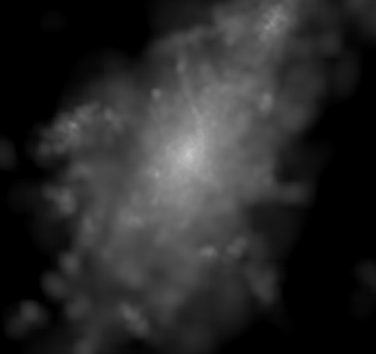
Figure 3.13: Surface density map of the DSC found in cluster D, when three values of $N_{\rm sm}$ are used (left panel) and when only one is used (right panel).

Figure 3.14: Velocity dispersions in the central part of cluster A, simulated at our higher resolution. Solid lines: stars belonging to SKID galaxies; long-dashed lines: DSC stars; dotted lines: DM particles; short-dashed lines: cD stars. Upper panel shows the results for the SKID analysis performed with a value of $\tau=20h^{-1}$ kpc, centre panel for $\tau=10h^{-1}$ kpc, lower panel for $\tau=6h^{-1}$ kpc.

The SKID algorithm works as follows:

• An overall density field is computed from the distribution of all available particle species, generally DM, gas and star particles. The density is estimated with a SPH spline–kernel, using a given number $N_{\rm sm}$ of neighbour particles. In the following we only include DM and star particles.

• The star particles are moved along the gradient of the density field in steps of $\tau/2$. When a particle begins to oscillate inside a sphere of radius $\tau/2$, it is stopped. In this way, $\tau$ can be interpreted as the typical size of the smallest resolved structure in the distribution of the star particles.

• When all star particles have been moved, they are grouped using a friends-of-friends (FOF) algorithm applied to the moved particle positions. The linking length is again $\tau/2$.

• The gravitational potential and binding energy of each group identified in this way is computed by accounting for all the particles inside a sphere centred on the centre of mass of the group and having radius $2\tau$ (for the moved star particles, their initial positions are used in the computation of the potential). The binding energies of individual particles are then used to remove from the group all the star particles which are recognised as unbound, in an iterative way: the centre of mass of the group and its potential are recomputed after a particle has been discarded.

• Finally, we retain such a SKID–group of stars as a galaxy if it contains at least 32 particles after the removal of unbound stars. The exact value of this number threshold is unimportant, but the smaller the threshold is, the higher is the probability of identifying as “galaxy” a random set of neighbouring star particles. Using 32 particles correspond to a mass threshold of $M=1.1\times 10^{10}h^{-1}M_{\odot}$ for the cosmological simulation.

The resulting set of objects identified by SKID depends on the choice of two parameters, namely $\tau$ and $N_{\rm sm}$. After many experiments and resorting to visual inspection in a number of cases, we find that a complete detection of bound stellar objects requires the use of a set of different values of $N_{\rm sm}$. Using only one value for $N_{\rm sm}$ results in “missing” some galaxies. We use $N_{\rm sm}=16,32,64$, and define a galaxy to be the set of star particles which belong to a SKID group for any one of the above $N_{\rm sm}$ values. If a star particle belongs to a SKID group for one value of $N_{\rm sm}$ and to another group for a different $N_{\rm sm}$, then the groups are joined and are considered as a single galaxy. All star particles not linked to any galaxies are considered to be part of the diffuse stellar component in the cluster. The left panel of Fig. 3.13 shows the surface density map of the DSC, as identified for our cluster D when all the three values of $N_{\rm sm}$ are used. In the right panel, we show the same map obtained using only $N_{\rm sm}=32$. In the latter, the bright spots correspond to “missed” galaxies.

$\tau$ roughly corresponds to the size of the smallest resolved structure, and we adopt

$$\tau\approx 3\epsilon$$

which is the scale where the softened force becomes equal to the Newtonian force. We have tested this choice by visual inspection in a number of clusters, and by performing an analysis of the velocity dispersions for the stars belonging to SKID galaxies and to the DSC. Fig. 3.14 shows the velocity dispersions for various components, namely the stars in galaxies, the stars in the DSC, the stars in the cD galaxy and the DM particles, for our cluster A (re-simulated at our higher resolution) when the value of $\tau$ is varied. The velocity dispersions are computed in spherical shells centred on the cluster centre, defined as the position of the DM particle having the minimum gravitational potential. For this high-resolution simulation, our fiducial choice is $\tau=6h^{-1}$ kpc. In the bottom panel of Fig. 3.14, the spikes in the velocity distribution of the stars in galaxies (the solid curve) at $R>100h^{-1}$ kpc correspond to SKID objects; no prominent spikes or bumps appear in the velocity dispersion profile for the DSC (long-dashed line), meaning that no structures in velocity that might correspond to “missed” galaxies are present in this component. Also, the value of the velocity dispersions for DSC and DM particles (dotted line) stay within $\approx 20$ % from each other, as expected when both component sample the same gravitational cluster potential.

When a larger value is used ($\tau=10h^{-1}$ kpc), spikes begins to appear in the DSC velocity dispersion curves, indicating that some objects, or part of them, are missed by the algorithm. This is especially clear for the spike at $R\approx 100h^{-1}$ kpc, which is present both in the velocity dispersion of stars in galaxies and in the velocity dispersion of the DSC, and clearly indicates that a fraction of stars in some galaxies have been mis-assigned to the diffuse component. Also, the discrepancy between DSC and DM velocity dispersions begins to grow, and the velocity dispersion of cD stars gets unrealistically large, $\sigma_{v}>500$ km/s. This happens because some low–speed DSC stars begin to be assigned to the cD, whose typical star particle velocities are even lower, thus increasing the velocity dispersion of the cD star population. The situation gets worse it the value of $\tau$ is increased to $20h^{-1}$ kpc.

We have performed a similar analysis on some clusters taken from our cosmological set, where the fiducial value from eq. (A.1) is $\tau=20h^{-1}$ kpc. Again, increasing $\tau$ to larger values results in having structures in the velocity space of the DSC, presumably due to missed objects. We conclude that the scaling (A.1) gives good results for the SKID galaxy identification, while keeping $\tau$ fixed to a given value (e.g. $20h^{-1}$ kpc) when the force resolution is varied is not a good choice.

When analysing particle distributions at redshift $z>0$, we keep fixed the value of $\tau$ in co-moving coordinates, thus allowing the minimum physical size of our object to decrease with increasing redshift. While this does not obey equation (A1), $\tau$ never becomes less than $\epsilon$. The effect is probably to slightly increase the amount of “volatile” galaxies at higher redshifts. Again, this choice was tested by visual inspection and by analysing the velocity dispersion distributions.

Also, we note that at high redshift ($z>1$) the distribution of gas particles inside star–forming proto–clusters often contains adjacent clumps of star particles. Applying SKID to such distribution results in “galaxies” composed of two or more of such clumps, which instead should be considered as separate galaxies. For this reason, we choose to use only DM and star particles for the galaxy identification.

Chapter 4 MUPPI - Multiphase particle integrator

In chapter 2, we presented various algorithms to include star formation and SN energy feedback in cosmological simulation (Sec. 2.3) and in semi-analytical models (Sec. 2.4). In this chapter, we present a novel algorithm, MUPPI (MUltiPhase Particle Integrator), a modified version of the Monaco 2004 (MO04, Sec. 2.4) analytic ISM, Star Formation and SNe feedback model, whose implementation in the GADGET-2 code (as a routine substituting the original star formation function, see Sec. 2.2.3) has been the principal work of the present PhD Thesis. The version of the GADGET code we use adopts an SPH formulation with entropy conserving integration and arithmetic symmetrisation of the hydrodynamical forces (see Sec. 2.2.2) and includes radiative cooling computed for a primordial plasma with vanishing metallicity.
One of the major problems of current simulations of galaxy formation is how to address the complex hydrodynamical processes in the multiphase interstellar medium (Ceverino & Klypin, 2008?). The insertion of a physically motivated model for star formation and SN feedback in place of a set of phenomenological recipes is the main novelty brought by MUPPI to the current SF models for simulations of galaxy formation. In MUPPI, in fact, the ISM dynamics depends only on local thermodynamical conditions, i.e. we don’t use equilibrium solutions to describe the ISM evolution. The “equilibrium” approach is instead taken for example in the GADGET-2 effective star formation model (Sec. 2.2.3). This means that MUPPI not only follows the non equilibrium phase at the onset of multi-phase regime, but also the response to changes in the local thermodynamics, e.g. pressure and/or temperature changes due to compressions/rarefactions and shocks. A detailed description is given in the following sections.
The organisation of the present chapter is as follows. In Sec. 4.1, we report how we initialise the model; in Sec. 4.2 we describe the model core and thus all the processes involved in regulating the ISM during and after star formation; finally, we account for the SNe energy redistribution in Sec. 4.3. In Appendix  4.A, we list the employed parameters; in Appendix  4.B we depict the flow chart of the MUPPI code and of the GADGET-2 code, highlighting the routines that have been changed by the MUPPI implementation.

4.1 Model equations and initialisation

The ISM gas is found in at least two forms: cold clouds of neutral atomic or molecular hydrogen and hot ionised hydrogen near hot young stars. These two inter-penetrating components have similar pressure but very different temperature and density ranges (McKee & Ostriker 1977, Efstathiou 2000).

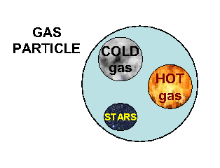
Figure 4.1: Schematic illustration of a MUPPI gas particle.

We follow the assumption that each gas particle is composed by a star component and by two gas phases, a hot and a cold one (denoted respectively by subscripts $h$ and $c$), which are in thermal pressure equilibrium, i.e.

$$n_{h}\cdot T_{h}=n_{c}\cdot T_{c}$$ (4.1)

Here and in the following $n$ denotes the number density, e.g. $n_{h}=M_{h}/(\mu_{h}\cdot mp)$, where $m_{p}$ is the proton mass, $\mu_{h}=4/(5\cdot f_{HI}+3)=0.6$ and $\mu_{c}=4./(3.\cdot f_{HI}+1.)=1.2$ are the molecular weights, with $f_{HI}$ the fraction of neutral hydrogen. Note that we kept the temperature of the cold phase fixed to $T_{c}=10^{3}$K. At a given timestep, a gas particle enters the multiphase regime if it full fills both a density, $\rho>\rho_{\rm thr}$, and a temperature threshold, $T<T_{\rm thr}$. In the present work, we adopt values of $\rho_{\rm thr}$ corresponding to a number density of $n_{\rm thr}$ = 0.25 cm^-3 and $T_{\rm thr}$ = $5\cdot 10^{4}$ K. Multiphase particle quantities are then initialised using the current values for the gas particle mass $M_{p}$, specific internal energy $E_{int}$ and volume

$$V_{p}=\frac{M_{p}}{\rho}$$ (4.2)

The hot and cold mass fraction ($F_{h}$= 0.999 and $F_{c}$ = 0.001) set initial values for the hot, $M_{h}$, and the cold mass, $M_{c}$. The particle should be completely in the hot phase at the onset of multi-phase regime; we set the value of $F_{c}$ to 0.001 only to avoid numerical instabilities in Ordinary Differential Equations (ODE) integration. Then, the initial temperature and, consequently, the energy of the hot phase are evaluated as:

$$T_{h}=\frac{E_{int}\cdot M_{p}}{\frac{3}{2}k\frac{M_{h}}{\mu_{h}m_{p}}}-\frac{M_{c}}{M_{h}}\frac{\mu_{h}}{\mu_{c}}T_{c}$$ (4.3)

$$E_{h}=\frac{3}{2}k\cdot\frac{M_{h}}{\mu_{h}m_{p}}T_{h}$$ (4.4)

At the first time step, MUPPI only performs initialisation, then the particle exits the model and goes back to GADGET. The next timestep, if it still fulfils the multiphase thresholds, it is allowed to enter the MUPPI core routine if the first exit condition is not met:

$$\rho_{out}<\frac{\rho_{\rm thr}}{1.5}\qquad\qquad\textrm{}$$ (4.5)

This is to avoid gas particles which are almost outside the star forming region (because part of a galactic fountain for example) to evolve the model and thus update their stellar mass component, besides all the other multiphase quantities. We verified, in fact, that without this exit condition, gas particles may spawn stars when they are already far away from the star forming region.
If no other exit conditions are met, a particle stays in the multi-phase stage for a time $t_{fin}$ = 2$t_{dyn}$, where $t_{dyn}$ is defined below (Eq. 4.17). After $t_{fin}$, the giant molecular cloud to which the particle belongs is considered to be destroyed. We use as an estimate of $t_{dyn}$ its value when the cold fraction reaches 99$\%$; after that Eq. 4.17describes the dynamical time of the rising molecular gas phase, rather than that of the parent GMC.

Similarly to MO04, we model the interplay among the three phases with a system of ODEs describing the various mass and energy flows which involve each phase. From the same work, we adopt the following equations:

$$\dot{M}_{\star}=\dot{M}_{SF}-\dot{M}_{re}\qquad\qquad\qquad\textrm{\small{MASS IN STARS}}$$ (4.6)

$$\dot{M}_{c}=\dot{M}_{cool}-\dot{M}_{sf}-\dot{M}_{ev}\qquad\qquad\textrm{\small{COLD MASS}}$$ (4.7)

$$\dot{M}_{h}=-\dot{M}_{cool}+\dot{M}_{re}+\dot{M}_{ev}\qquad\qquad\textrm{\small{HOT MASS}}$$ (4.8)

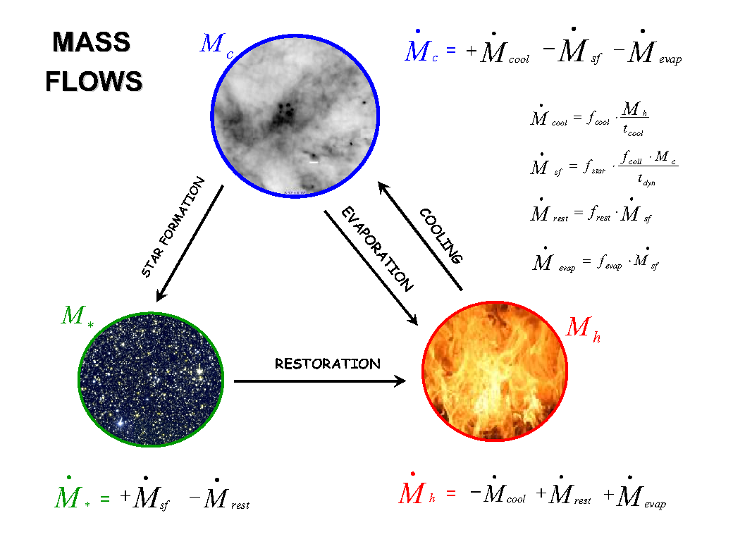
Figure 4.2: Schematic illustration of the mass flows between the different phases.

A schematic view of the mass flows among the different phases is given in Fig. 4.2.
The energy of the cold phase is kept constant at a temperature $T=100K$. The energy of the hot phase instead evolves according to:

$$\dot{E}_{h}=\dot{E}_{SN}-\dot{E}_{cool}+\dot{E}_{hyd}\qquad\qquad$$ (4.9)

where the first term on the right hand side describes the non-gravitational energy injected by exploding supernovae, the second term the radiative energy losses by cooling ($\dot{E}_{cool}=E_{h}/t_{cool}$) and the third term the energy change due to the hydrodynamics, introduced by the thermodynamical conditions of the medium after the gas particles evolved of our model (see Sec. 4.2.5).
We describe each term of the above equations ( 4.6 -  4.9) in the next sections.

4.2 Model core

After initialisation, the multiphase gas particle evolution is followed by integrating the ODEs for mass and energy flows using an adaptive step size fourth-order Runge-Kutta (RK4) algorithm. The RK4 routine propagates a solution over an interval ($x_{2}-x_{1}$) by combining the informations from several Euler-style steps and then using this information to match a Taylor series expansion up to some higher order (see e.g “Numerical recipes in C. The art of scientific computing” for a technical account). The integration is taken from $x_{1}=0$ to the current GADGET timestep $x_{2}=\Delta t$ with initial stepsize $h=\Delta t/100$. In particular situation, it could happen that the RK4 stepsize becomes similar to the cooling time, $t_{cool}$, thus compromising the code ability in closely follow the hydrodynamical changes. Therefore before entering the RK4 routine, we check if $h>t_{cool}/5$, then the stepsize is set to $h=t_{cool}/5$.
Once inside the RK4 derivative function, the code computes over the timestep $h$ the solutions $M_{c}$, $M_{c}$, $M_{*}$ and $E_{h}$ to the MUPPI differential equations describing star formation and feedback related physics. This is achieved at first by directly computing the current values for the following quantities: the hot and cold filling factors,

$$f_{h}=\frac{1}{1.0+\frac{F_{c}}{F_{h}}\cdot\frac{\mu_{h}}{\mu_{c}}\cdot\frac{T_{c}}{T_{h}}}\qquad\qquad f_{c}=1-f_{h}$$ (4.10)

the volumes occupied by the hot and the cold phases,

$$V_{h}=V_{p}\cdot f_{h}\qquad\qquad V_{c}=V_{p}\cdot f_{c}$$ (4.11)

and finally the densities of the hot and cold component

$$\rho_{h}=M_{h}/V_{h}\qquad\qquad\rho_{c}=M_{c}/V_{c}$$ (4.12)

We use the GNU-Scientific Libraries (GSL) to perform the integration over the whole code timestep $\Delta T$. When convergence is reached, the model exits the RK4 routine and goes back to the main code. During such integration, two more exit conditions are posed:

$$M_{h}<M_{c}/10^{9}\qquad\qquad$$ (4.13)

which check if the gas particle is “freezing”, thus becoming depleted of hot phase and not able to sustain a multi-phase gas anymore, and

$$f_{c}<10^{-18}\qquad\qquad$$ (4.14)

which controls if the gas particle is depleted of the cold phase. If these cases are true, the gas particle exists the RK4 routine and goes back to the main code. Soon after, all its multiphase quantities are set at zero and the particle exits MUPPI.

In the next paragraphs, we describe the physical processes and flows between the gas phases and the star mass.

4.2.1 The formation of molecular clouds

The original MO04 paper tries to model the formation of giant molecular clouds (GMC). In numerical simulations, often one gas particle has a mass lower than that of a typical GMC, and thus it makes no sense to follow the formation of GMCs inside it. Thus, we use instead a phenomenological prescription for describing the amount of molecular gas and the consequent star formation.

Blitz & Rosolowsky (2006) showed that the ratio of atomic to molecular gas in galaxies is primarily determined by the interstellar gas pressure $P_{ext}$. Following their work, the fraction $f_{\rm mol}$ of atomic hydrogen (which is directly connected with the star formation rate) present in the cold phase is calculated as:

$$f_{\rm mol}=\frac{1}{1+4(\frac{P_{0}}{P_{ext}})}$$ (4.15)

where $P_{0}=10^{4}$ (normalised to observed values found in the Milky Way) and $P_{ext}=P_{th}+P_{kin}$ is the total pressure exerted by the gas on the ISM. The thermal pressure $P_{th}$ is mainly powered by the thermal energy injected by SN explosions (Mc Low 2002) while the kinetic term $P_{kin}$ is mainly driven by cold cloud turbulence. We modelled the kinetic pressure in MUPPI with a simple prescription, thus considering separate contributions from thermal and kinetic pressure, and verified that results are substantially unchanged with respect to the formulation ( 4.15). We dropped such kinetic pressure model not to add one more free parameter in MUPPI.

4.2.2 Star formation

Once the fraction $f_{\rm mol}$ has been computed, star formation begins. The rate at which cold gas transforms into stars, i.e. the star formation rate (SFR), is evaluated as:

$$\dot{M}_{SF}=f_{\star}\cdot\frac{f_{\rm mol}\cdot M_{c}}{t_{dyn}}$$ (4.16)

where $f_{\star}$ gives the fraction of star forming gas effectively converted into stars. The fraction $f_{\rm mol}$ multiplied by the cold mass $M_{c}$ gives the amount of gas available for star formation, i.e. the molecular gas, $M_{mol}$. We assume that star formation proceeds on the order of the dynamical time given by:

$$t_{dyn}=\sqrt{\frac{3\pi}{32G\rho_{\rm c}}}\backsimeq 5.15\cdot 10^{7}\sqrt{\mu_{c}\cdot n_{c}}yr$$ (4.17)

A fraction $f_{re}$ (0.2 in our runs) of cold gas involved in star formation is immediately restored to the hot phase:

$$\dot{M}_{re}=f_{re}\cdot\dot{M}_{SF}$$ (4.18)

Note that here we just build up stellar mass, we don’t spawn star particles. This is eventually done after exiting the MUPPI routine, when the computation goes back to GADGET and the probabilistic method described by Eq. 2.31 is invoked to form new star particles. The star formation rate calculated by MUPPI is adopted in the probabilistic method.

4.2.3 The cold and the hot masses

The replenishment of the cold phase is counteracted by star formation (Eq. 4.16), which depletes the cold gas reservoir, and by evaporation of the cold collapsing gas back to the hot phase due to SN explosions.
The rate at which gas cools from the hot phase is assumed to be:

$$\dot{M}_{cool}=\frac{M_{h}}{t_{cool}}$$ (4.19)

where $t_{cool}$ is the radiative cooling time derived from the GADGET-2 cooling function which uses tabulated cooling rates given by Sutherland & Dopita (1993). If the multiphase gas particle under exam has a temperature lower than $T=10^{4}K$, we fit the cooling time with the following expression:

$$t_{cool}^{fit}=t_{cool}\cdot(\frac{T}{T_{cf,0}})^{-3}$$ (4.20)

where $T_{cf,0}=1.78\cdot 10^{4}K$. We made this approximation because the original GADGET cooling function dies at $T=10^{4}K$.

A future development of MUPPI will consist in consistently including molecular and atomic cooling, down to $T$ = 100 K. Moreover, when metallicity of gas will be available thanks to the integration of MUPPI with the chemical evolution model implemented by Tornatore et al. 2004 and already present in the code, we will also include the dependence of gas cooling upon its metallicity. The fit implemented here to follow cooling at temperatures lower than 1000 K is only needed to avoid instabilities at the onset of multi-phase regime, when the particle may have low temperatures and the energy feedback from SNe is not yet active. We verified that using different kind of fits doesn’t substantially change our results.

As a first source of early SN feedback, we suppose that collapsing clouds are evaporated back to the hot phase by exploding supernovae with a rate given by:

$$\dot{M}_{ev}=f_{ev}\cdot\dot{M}_{SF}$$ (4.21)

where $f_{ev}$ is 0.1 in our runs. This term is inserted in the equation regulating the hot gas mass evolution in order to take into account the effects of thermal conduction at the interface between the cold and the hot mass. Again, the integration of MUPPI and the Tornatore et al. 2004 scheme will allow us to also consider SNIa energy contribution to the hot phase.

4.2.4 Supernova feedback energy

We suppose that SNe exploding within a star forming gas particle give rise to a super-bubble which propagates in the more pervasive hot phase. As previously depicted in Sec. 2.4.1, we consider two possible feedback regimes following naturally from this setting: the pressure confinement regime, modulated by the fraction $f_{\rm fb,i}$, which gives the amount of thermal energy stopped by the external pressure within the star forming gas particle and the blow out regime, modulated by the parameter $f_{\rm fb,o}$, which describes the energy blowing out of the gas particle which is redistributed among neighbours.
The redistribution of the fraction $f_{\rm fb,o}$ of energy which blows outside the particle is treated by a separate routine, called just after MUPPI (see Sec. 4.3).
In the ODE integrator core, we thus take into account only the fraction of SN energy which remains trapped inside the star forming particle. The heating rate due to SNe is:

$$\dot{E}_{SN}=E_{51}\cdot f_{\rm fb,i}\cdot\frac{\dot{M}_{sf}}{M_{\star,sn}}$$ (4.22)

where $E_{51}=10^{51}$ erg is the canonical value for the energy released by one supernova and $M_{\star,sn}=120M_{\odot}$ is the mass of formed stars per SN.

4.2.5 The SPH/model interface and the term $\dot{E}_{hydro}$

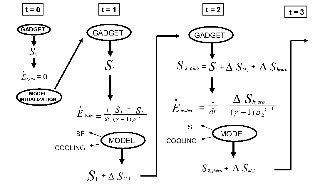
Figure 4.3: Schematic illustration of the interaction of MUPPI with the GADGET SPH; see text for details.

Star formation and cooling change the hydrodynamical conditions of the multiphase particle after the ODE integration. We thus need to introduce a term in which we can store these changes to later inform the SPH.
When a gas particle with entropy $S_{n}$ fulfils the multiphase thresholds and enters MUPPI, its entropy is updated to $S_{n}+\Delta S_{muppi}$. The term $\Delta S_{muppi}$ is evaluated from the mass weighted average energy $E_{ave}$ of the hot and the cold phases, given by:

$$E_{ave}=k\cdot\frac{T_{ave}}{(\gamma-1)\cdot\mu_{med}\cdot m_{p}}$$ (4.23)

where

$$T_{ave}=\frac{\mu_{med}}{M_{c}+M_{h}}\cdot\frac{M_{h}\cdot T_{h}}{\mu_{h}}\frac{M_{c}\cdot T_{c}}{\mu_{c}}$$ (4.24)

and $\mu_{med}=(\mu_{c}\cdot M_{c}+\mu_{h}\cdot M_{h})/(M_{c}+M_{h})$.

At the following timestep ($n+1$) the SPH evaluates the new thermodynamical conditions of the medium $S_{n+1}$, increasing thus the entropy by:

$$\Delta S_{hyd}=S_{n+1}-S_{n}-\Delta S_{muppi}$$ (4.25)

The rate of energy change due to the hydrodynamics is thus:

$$\dot{E}_{hyd}=\frac{1}{dt}\frac{\Delta S_{hyd}}{(\gamma-1)\rho^{\gamma-1}}$$ (4.26)

where $\gamma$ is the adiabatic index. The term $1/(\gamma-1)\rho^{\gamma-1}$ is the SPH factor to convert entropies into energies. The term $\Delta S_{muppi}$ is subtracted in the evaluation of Eq. 4.25 because it would otherwise be computed twice, at timestep $n-1$ directly by MUPPI, and at timestep $n$ since included in $\Delta S_{hyd}$. We note that gas entropy changes in the entropy conserving version of GADGET can happen due to two processes: viscous energy dumping, caused by the artificial viscosity, and hydrodynamic variations in pressure and temperature, due to interaction with surrounding particles. The latter process is physical, e.g. it is extreme during shocks. This term is the one which enables MUPPI to respond to the local hydrodynamical properties of the gas and to their evolution. For a schematic representation, see Fig. 4.3.

4.3 Final steps: storing and redistributing the “blow-out regime” energy

After having found the solutions to the system of ODEs, the computation proceeds in the main code by computing the amount of SNe energy that blows outside the particle (“blow-out regime”) and thus has to be redistributed among particle neighbours.
The total out-flowing thermal energy per particle that needs to be redistributed at a given timestep is calculated as:

$$\Delta E_{SN,o}=E_{51}\cdot f_{\rm fb,o}\cdot\frac{\Delta M_{sf}}{M_{\star,sn}}$$ (4.27)

where $E_{51}=10^{51}$ erg is the energy released by one supernova, $\Delta M_{sf}$ is the mass in stars formed in the timestep and $M_{\star,sn}=120M_{\odot}$ is the mass of formed stars per SN.
Before exiting the main code, we update the SPH entropy by considering the change in internal energy introduced by the evolution of the model core. Afterwards, the code goes back to GADGET and later to the function to redistribute the blow out energy is called.

4.3.1 Thermal energy redistribution

Following the SPH formalism, we define neighbouring particles as those lying within the sphere of radius given by the star forming particle smoothing radius $h_{\star}$. For each SN explosion event, the maximum number of particles that can receive the SN energy is fixed by the number of SPH neighbours ($N_{ngb}=32$). Among the SPH neighbours, we select those which lie within the cone with vertex at the star forming gas particle, axis parallel to the local density gradient $\vec{\nabla}\rho$ and aperture $2\theta=140\pi$ (see Fig. 4.4).

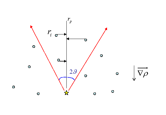
Figure 4.4: Schematic illustration of the energy redistribution mechanism.

We then distribute the energy $\Delta E_{SN,o}$ on the basis of the distance from the neighbour $i$ to the straight line $r_{\vec{\rho}}$, traced by the star forming particle in the opposite direction of the local density gradient. We choose this scheme of energy redistribution to mimic the hot gas flow along the direction of smallest resistance. For simplicity, we only computed the energy exchange and drop the mass flow.

With this scheme, each particle keeps part of its SN energy and gives another part to its neighbours. Thus, the pressure confinement or blow out regime are accounted for by the spatial distribution of particles. In the centre of a disk, for example, particles are heated up by neighbours, their temperature increases, and as a consequence they would tend to evaporate by buoyancy. But they are confined by the pressure of other particle of the disk and the energy stays localised. At the boundary of the disk, a particle taking energy will not be confined, thus it will evaporate, with a velocity which depend by the energy it gains. We will show examples of this process in the next Chapter. We also implemented other energy redistribution schemes, e.g. we tried to assign energy isotropically, or to all neighbours which resides in the semi-sphere opposed to the density gradient. The scheme described here has shown to be the most effective in reproducing the confinement/blow out behaviours of the heated gas. Also, we tried different energy assignment kernel; for example, using the distance from the star forming particle centre instead of $r_{p}$ in Eq. 4.28. Within one energy redistribution scheme, changing the relative energy given to each neighbours does not influence our results.

The SN energy fraction received by a neighbour $i$ is computed as:

$$\Delta E_{SN,i}=\frac{m_{i}\cdot W(|r_{i}-r_{\vec{\rho}}|,h_{\star})\Delta E_{SN,o}}{\rho_{i}}$$ (4.28)

Note that we use the same SPH kernel used in the hydrodynamical calculations, and therefore farther particles get an energy fraction which is significantly lower than the ones lying closer the density gradient vector $r_{\vec{\rho}}$.

4.4 Summary

In this Chapter we have presented MUPPI, MUltiPhase Particle Integrator, our original sub-grid model of the Inter Stellar Medium (ISM) based on the analytical model by Monaco 2004 (see Sec. 2.4), which has been implemented on top of the GADGET-2 code (see Chapter 2, Sec. 2.2).
An illustration of changes in the GADGET code is given in Fig. 4.5; we completely re-wrote the star formation and cooling function, while changes in the hydrodynamics and time stepping functions are less important.

The main feature of this model is that it does not use equilibrium solutions for the ISM evolution (as instead does the original GADGET star formation routine) but, rather, it assumes the ISM dynamics depends only on local properties. Each gas particle, in fact, evolves the model and all its equations by its own: the differential equations for mass and energy flows are thus solved taking in direct account the local thermodynamic conditions.
Of course, since MUPPI changes the thermodynamical properties of gas particles, the SNe energy injection also influences the SPH part of the code. Gas cooling is treated by MUPPI, and only the hot phase gas can cool, thus SNe energy is ṉot immediately radiated away in our model. In fact, the hot phase density is typically very low, since the majority of the gas mass is in the cold phase (see next Chapter); cooling is not very efficient in this condition. Moreover, the hot phase is conserved from a time step to the next one and its physical evolution is computed; e.g., SH03 effective model instead re-evaluate the equilibrium, thus allowing a lot of gas to change its phase as a consequence of SNe energy injection. This makes MUPPI feedback process self consistent and quite effective without the need of introducing an ad-hoc kinetic energy injection.

The implemented chain of processes are as as follows:

• Each gas particle is assumed to be made of hot gas, cold gas and stars where gas phases are in pressure equilibrium;

• The amount of gas available for star formation is given by a phenomenological prescription proportional to the thermal pressure (Blitz & Rosolowsky, 2006)

• The star formation rate gives the number of SNII, whose energy is partly given to the hot phase.

• The evolution of the system is obtained by numerically integrating the system of equation for the mass and energy flows.

• SN energy is released both inside and outside each gas particles. The redistribution of out-flowing energy to neighbouring particles takes place along the least resistance path.

Appendix 4.A APPENDIX I: List of parameters

$n_{h}$ / $n_{c}$	hot/cold number density
$T_{h}$ / $T_{c}$	hot/cold temperature
$m_{p}$	Proton mass
$f_{HI}$	fraction of neutral hydrogen
$\rho_{thr}$	density threshold for multiphase state
$T_{thr}$	temperature threshold for multiphase state
$n_{thr}$	number density threshold for multiphase state
$V_{p}$	total volume of the gas particle
$V_{h}$ / $V_{c}$	hot/cold volume
$M_{h}$ / $M_{c}$	hot/cold phase mass
$F_{h}$ / $F_{c}$	hot/cold mass fraction
$\mu_{h}$ / $\mu_{c}$	hot/cold phase molecular weight
$E_{int}$	internal energy coming from GADGET
$k$	Boltzmann constant
$\rho$	total density of the gas particle
$t_{cool}$	cooling time
$f_{h}$ / $f_{c}$	hot/cold filling factors
$f_{\rm mol}$	fraction of atomic hydrogen
$P_{0}$	pressure normalised to the Milky Way
$P_{ext}$	total pressure (here just thermal)

$M_{*}$	mass in stars
$\dot{M_{*}}$	rate of change of the mass in stars
$\dot{M_{SF}}$	star formation rate
$f_{*}$	efficiency of star formation
$t_{dyn}$	dynamical time
$\dot{M_{re}}$	restoration rate
$f_{re}$	fraction of restored mass
$\dot{M_{cool}}$	cooling rate
$t_{cool}^{fit}$	fit to the cooling time data
$\dot{M_{ev}}$	evaporation rate
$f_{ev}$	evaporated fraction of the star forming cloud
$\dot{E_{SN}}$	SNe heating rate
$f_{\rm fb,i}$	fraction of SNe energy trapped inside the gas particle
$f_{\rm fb,o}$	fraction of SNe energy blowing outside the gas particle
$\dot{M_{\star,sn}}$	mass of formed star per SN
$\dot{M_{c}}$	rate of change of cold mass
$\dot{M_{h}}$	rate of change of hot mass
$\dot{E_{h}}$	net of energy flux of the hot phase
$\dot{E_{cool}}$	rate of energy loss by cooling
$\dot{E_{hyd}}$	rate of energy change due to hydrodynamics
$\Delta E_{SN,o}$	SNe energy to be redistributed in the timestep
$\Delta M_{sf}$	mass in stars formed in the timestep
$\Delta E_{SN,i}$	SNe energy received by neighbour $i$ in the timestep

Appendix 4.B APPENDIX II: Flow charts

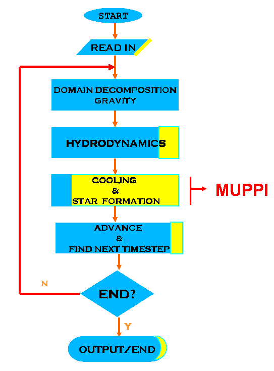
Figure 4.5: Flow chart of the GADGET-2 code. In yellow we highlight how much of the selected routine has been changed due to the insertion of the MUPPI model.

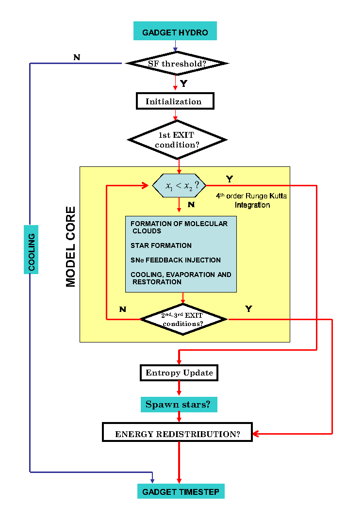
Figure 4.6: Flow chart of the MUPPI code. The illustrated processes are fully described along the present chapter. In particular, processes depicted above the “model core” section are outlined in Sec. 4.1; the model core processes are described in Sec. 4.2.2; the last part is accounted in Sec. 4.3.

Chapter 5 Results

In this section, we present and discuss the results obtained from a set of simulations (see Table  5.1) performed with the code described in Chapter  4. The discussion proceeds as follows. Since one of the fundamental properties that a star formation and feedback model must be able to reproduce is that in Milky Way (MW) like simulations, properties of simulated interstellar medium (ISM) must reproduce observations; in Sec. 5.2 we describe the simulation runs conducted with a MW model and we describe the resulting behaviour. In order to test the MUPPI code behaviour on different initial physical conditions, in Sec. 5.3 we describe the simulations runs done using a dwarf galaxy like model (DW) and two isolated halos, one typical of the MW (CFMW) and one of a dwarf galaxy (CFDW). These last two runs have been carried on to verify if our code works well in very different physical conditions such those found at the centre of cooling flows. We also use a more massive halo, with mass $M$ = $10^{13}M_{\odot}$, which we already described in Chapter 2. In Sec. 5.5 we discuss the simulations conducted with the purpose of assessing the stability of our results with respect to the details of the implementation and to the resolution. In particular we simulated the CFDW with ten times more (HR) and ten times less (LR) gas and dark matter particles (see Tab. 5.1), and the MW in LR. Finally we discuss and summarise our conclusion in Sec. 5.6.

	$f_{fb_{0}}$				$n_{thr}$ [cm${}^{-3}]$				$f_{\rm fb,i}$	$f_{\star}$		res			GDT
	0.0	0.3	0.7		0.05	0.1	0.25		0.05	0.1		HR	LR		EFF	EFF+wind
MW	$\bigstar$	$\bigstar$	$\bigstar$		$\bigstar$	$\bigstar$	$\bigstar$		$\bigstar$	$\bigstar$			$\bigstar$		$\bigstar$	$\bigstar$
CFMW	$\bigstar$	$\bigstar$	$\bigstar$				$\bigstar$
DW	$\bigstar$	$\bigstar$	$\bigstar$		$\bigstar$	$\bigstar$	$\bigstar$									$\bigstar$
CFDW	$\bigstar$	$\bigstar$	$\bigstar$				$\bigstar$					$\bigstar$	$\bigstar$		$\bigstar$	$\bigstar$

Table 5.1: Simulation summary. We show the labels of the initial condition models (see Sec.5.1) vs the characteristics of the simulation runs: the model parameters that have been varied ($f_{fb_{0}}$, $n_{thr}$, $f_{\rm fb,i}$ and $f_{\star}$), the numerical tests done with varying resolution (HR: 10 times better mass resolutionl LR: ten times worse mass resolution) and finally runs done with the original GADGET SF code, with (EFF+wind) and without (EFF) winds (see Sec. 2.2.3).

5.1 Initial Conditions (ICs)

5.1.1 Isolated galaxy models (MW, DW)

Testing the effect of sub-grid models in galaxy formation simulations is best done in numerical realizations of isolated galaxies. These models are constructed on purpose to resemble observed galaxies, with a disk of gas and stars, and optionally a stellar bulge, all embedded in an extended dark matter halo with structural properties (e.g. mass, spin, density profile) consistent with cosmological simulations of the hierarchical growth of CDM halos.
The galaxy models used in this work have been created by Simone Callegari, following the prescription depicted in Springel, Di Matteo & Hernquist 2005. In what follows we review their basic features, for a full description see the referenced paper.
Both MW and DW are generated with near equilibrium distributions of collisionless particles consisting in rotationally supported disc of gas and stars (with spin parameter $\lambda$), a star bulge (not in DW) and a dark matter halo. These different structural components are described by independent parameters (see Tab.). The halo dark matter mass distribution of both MW and DW galaxy models has been modelled with an Hernquist (1990) profile. The disc components of gas and stars have been modellel with an exponential surface density profile having scalelenght $r_{s,d}$. The total mass of the disc, $M_{disk}$, has been computed as a fraction of the total mass of the galaxy. The MW model has also of a spherical star bulge, modelled with an Herquist profile. The bulge scalelenght $r_{s,b}$ is treated as a free parameter parametrized in units of $r_{s,d}$, while the bulge mass $M_{bul}$ is specified as a fraction of the total galaxy mass. In both galaxy models, a fraction $f_{gas}$ of the disc is assumed to be in gaseseos form, the rest in stellar form.

We evolved all galaxy model with non-radiative physics only, i.e. no cooling and star formation, for 10 dynamical times, and verified that our models are numerically stable. We use the non-radiatively evolved models after 4 dynamical times as initial conditions for MUPPI, so as to be sure that MUPPI evolution is not polluted by numerical instabilities.

	$f_{bar}$	$r_{s,d}$	$M_{disk}$	$r_{s,b}$	$M_{bul}$	$f_{gas}$	$\lambda$
MW	0.06	2.9	$2.6\cdot 10^{10}$	0.58	$6.6\cdot 10^{9}$	0.1	0.04
DW	0.05	3.5	$5.6\cdot 10^{9}$	0	0	0.2	0.04

Table 5.2: Main properties of the galaxy models. Column 1: galaxy name. Column 2: radial disc scalelenght in Kpc. Column 3: total mass in the disc (gas + stars) in $M_{\odot}$. Column 4: bulge scalelenght in Kpc. Column 5: mass in the bulge in $M_{\odot}$. Column 6: gas fraction in the disc. Column 7: spin parameter.

5.1.2 Isolated halos (CFMW, CFDW)

The procedure used to generate the initial conditions for the isolated, non-rotating halos is the same reported at the beginning of Sec. 2.5.2. We use a NFW density profile for the DM distribution, instead of an Hernquist one, since the former is suggested by cosmological simulation. We refer the reader to Chap.2 for a full description on the halo ICs generation.

	$M_{200}$	$r_{200}$	$c_{\rm NFW}$	$m_{\rm DM}$	$m_{\rm gas}$
CFMW	$6.6\cdot 10^{11}$	197	12	$3.1\cdot 10^{6}$	$4.2\cdot 10^{5}$
CFDW	$1.1\cdot 10^{11}$	80	13	$5.7\cdot 10^{5}$	$1.4\cdot 10^{5}$

Table 5.3: Main properties of the simulated halos. See Sec. 2.5.2 and text for more significant details. Column 1: halo name. Column 2: mass enclosed in within $r_{200}$ in $M_{\odot}$. Column 3: value of $r_{200}$ in kpc. Column 4: NFW concentration. Column 5: mass of a DM particle in $M_{\odot}$. Column 6: mass of a gas particle in $M_{\odot}$.

With the procedure depicted in Chapter 2, we generated two halos, having the same DM and barionic mass of the Milky Way (CFMW) and of a dwarf galaxy (CFDW); see Tab. 5.3 for a summary on halos main properties. CFMW halo is sampled with 2.5 x $10^{5}$ DM and 1 x $10^{5}$ gas particles inside $r_{200}$, while CFDW with 1.9 x $10^{5}$ DM and 5 x $10^{4}$ gas particles inside $r_{200}$. The baryon fraction is $f_{\rm bar}$=0.05 in CFMW and $f_{\rm bar}$=0.06 in CFDW. We set the Plummer-equivalent softening, following Power et al. 2003, to be $1$ kpc in CFMW and $0.6$ kpc in CFDW for the DM and half those values for the gas. We further assume the minimum value for the SPH smoothing length to be 0.5 times that of the gravitational softening. The number of the SPH neighbours has been set to $N_{\rm ngb}$ to be 32. In all runs we set the initial angular momentum to zero.

We evolved the CFDW runs for 5.5 Gyr, while the CFMW runs have been evolved just for 1 Gyr due to the higher computational cost.

$n_{thr}$	$T_{thr}$	$f_{\star}$	$f_{ev}$	$f_{\rm re}$	$T_{c}$	$t_{\rm fin}$	$P_{0}$	$f_{b_{\rm in}}$	$f_{b_{\rm out}}$
0.25	5 $\cdot 10^{4}$	0.01	0.1	0.2	1000	2$t_{dyn}$	1000	0.02	0.3

Table 5.4: Reference set of parameters. Column 1: number density threshold in cm^-3. Column 2: temperature threshold in K. Column 3: star formation efficiency. Column 4: evaporated fraction of cold cloud. Column 5: restored mass fraction. Column 6: temperature of the cold phase. Column 7: exit condition from the multi-phase state. Column 8: external pressure normalization. Column 9: fraction of SN energy feedback trapped inside the particle. Column 10: fraction of SN energy feedback blowing outside the particle.

5.2 Milky Way

In this section we investigate te effects of MUPPI on simulations of the MW model runned with our reference set of MUPPI parameters (see Tab. 5.4). Here we want to describe the behaviour of the gas when MUPPI is used. We will discuss only the effect of varying $f_{\rm fb,o}$ in this section: a parameter study will be presented in Sec. 5.4.

5.2.1 The Inter Stellar Medium

We start by showing the evolution of the thermodynamical properties of single gas particles lying (a) in the centre of the galaxy and (b) on the disc, at the edge of the star forming region (see Fig. 5.1).

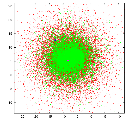
Figure 5.1: The distribution of stars (green) and gas (red) in the xy plane in the initial conditions for simulation of the MW galaxy where we highlight the position of the core (purple) and disc (blue) multi-phase particles studied in Sec.  5.2.1

In Fig. 5.2, we show properties of the central gas particle and in Fig. 5.3 those of the disc gas particle.
At the onset of the simulation, the gas particles undergo a rapid collapse as the cooling begins to act. As soon as the core gas particle fulfills the star formation thresholds and enters MUPPI, its initially hot gas rapidly cools and feeds the cold phase. This is clearly shown by the top panel of Fig. 5.2 where we plot the evolution of the cold, hot and stellar mass. Corresponding to the rapid filling of the cold phase (which soon reaches an equilibrium value) and to the increase of the molecular gas fraction, shown in the central panel, the stellar mass undergoes a fast growth and thus a substantial amount of SNe energy feedback is injected in the medium. This causes a quick jump in the particle hot phase temperature and pressure (shown in the second panel from the top), which respectively reaches $T_{h}\sim 10^{7}$ K and $P/K=7\cdot 10^{4}$ K cm^-3.

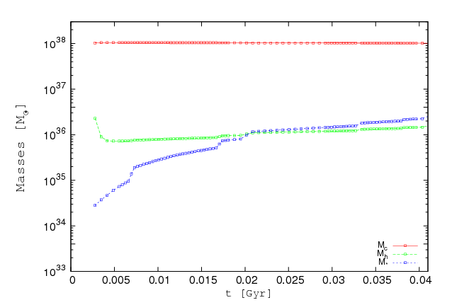
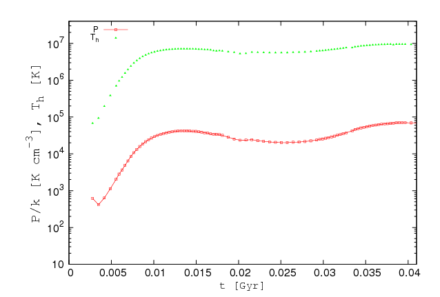
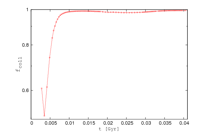
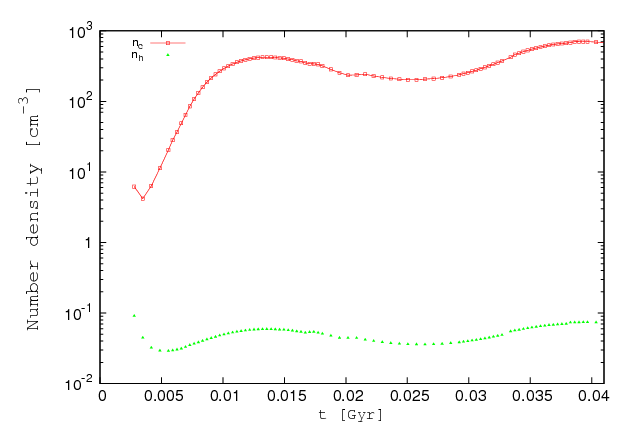
Figure 5.2: The ISM evolution of a gas particle lying in the galaxy core. From the top to bottom, the panels shows the evolution of the cold, hot and star masses in $M_{\odot}$ (first panel); the hot phase temperature in $K$ and the pressure in $Kcm^{-3}$ (second panel); the fraction of molecular gas (middle panel); the gas particle volume in $cm^{3}$ (second-last panel); the cold and the hot number densities in $cm^{-3}$ (bottom panel). See Sec. 5.2.1 for details.

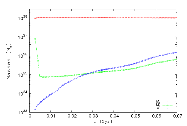
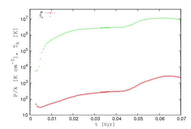
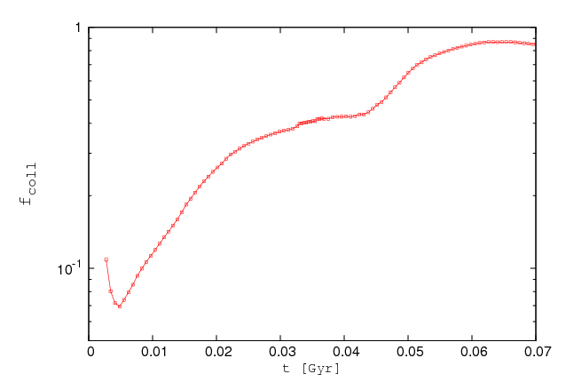
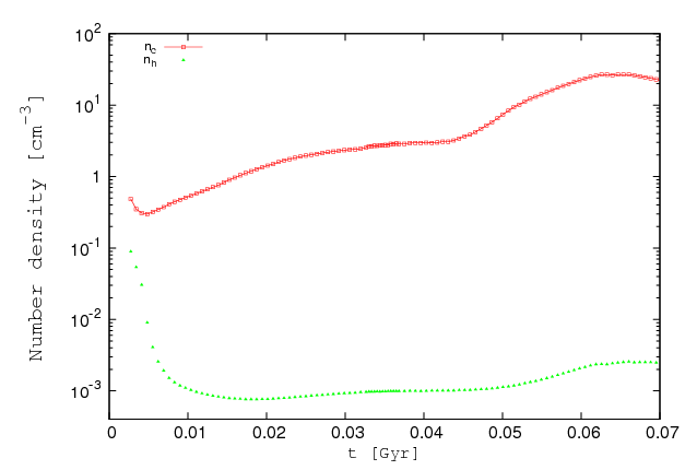
Figure 5.3: Same as in Fig. 5.2 but for a gas particle lying in the disc.

In the third panel from the top, we show the evolution of the fraction of molecular gas ($f_{coll}$, Eq. 4.15): after a sudden decay corresponding to the initial lack of pressure support, this fraction rapidly increases with the pressure and stabilises to a value around unity, with small fluctuations due to the pressure changes. This means that, for this particle, all the cold gas is in the molecular, star-forming form. This is due to the higher value of $P/K$, which is between 10⁴ and 10⁵ K cm^-3. The plot of Fig. 5.2 clearly show how the physics of the ISM inside the particle is driven by the pressure. When $P/K$ increases, $f_{coll}$ and $n_{c}$ increase, giving an higher star formation rate and consequently a stronger energy feedback which causes the temperature of the hot phase to also increase.
On the other hand, the pressure responds to volume changes as it can be seen by comparing trends in the second and in the fourth panel. When volume decreases (compression) the pressure increases and vice-versa. But the volume, as defined by Eq. 4.2, is determined by the SPH evolution; here we have the mechanism which causes the response of the ISM to the local hydrodynamics. In the bottom panel, we show the evolution of the cold and hot number density: the cold one rises as the cold phase is feeded by cooling of hot gas; on the other side the hot number density diminishes. The whole multi-phase stage lasts $\sim$ 40 Myr, then the particle exits the multi-phase regime as imposed by our exit condition (see Sec. 4.1).

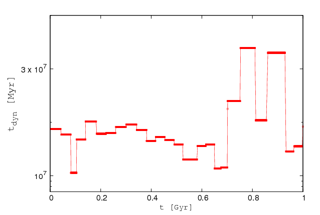
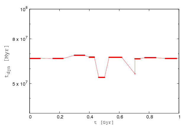
Figure 5.4: Dynamical timescale in Myr for a gas particle residing in the galaxy core (left panel) and for a gas particle in the disc (right panel), in different multi-phase stages during a period of $1$ Gyr.

As depicted in Fig. 5.3, the typical evolution of a gas particle lying in the disc is characterised by a different behaviour with respect to a gas particle lying in the dense central galaxy regions. First of all, being the particle in a colder and less dense zone, its cold phase forms in more timesteps (even if this effect is small), while the general interchange between the various mass phases is instead analogous. The particle pressure (second panel) results much less smaller than that in “core” case. Values of $P/K$, $n_{h}$, $n_{c}$ for this case resamble those observed in the solar neighbourhood. The gas particle we chose is at 6.2 Kpx from the galaxy center. Note that the model generated such an ISM behaviour self-consistently; we don’t impose particular values for $P/K$, $n_{h}$ and $n_{c}$. After 30 Myr since the gas particle entered in multi-phase stage, the volume decreases causing a small increase in pressure which then stays almost constant. Thus star formation increases giving some SNe feedback. This could be due e.g to a spiral arm passing through the position of the particle. The pressure wave causes a rapid increases in the fraction of molecular gas (middle panel) and in the cold number density (bottom panel).

After about 50 Myr, the pressure shows a more significant increase due to the slow piling up of thermal energy given by the star formation. The hot mass increases and this pressurize the particle. The local thermodynamics is not responsable for this effect: from the fourth panel, we can see taht the particle is in an expansion phase. At this point, the star formation boosts and further pressurize the particle, until, at the very end of the multi-phase stage, an expansion driven by the SPH stops the runaway process Such an expansion is caused by MUPPI itself. In fact, this gas particle has an average distance of 0.35 Kpc from the disc plane, and (almost) does not move form this position. Towards the end of the mulit-phase stage, it has an high temperature and enough mass in the hot phase to cause it to flow away from the disc. At the end of the multi-phase stage its distance from the disc plane is already of 0.49 Kpc and the particle has “gone into wind”.
Finally we show in Fig. 5.4, the behaviour of the dynamical time over one Gyr in both the above cases. Both particles enter the multi-phase stage several times during this period. The central gas particle dynamical time takes values between 10 and 30 Myr and it is subjected to changes from one multi-phase stage to the following. On the contrary, the disc gas particle dynamical time is between 50 and 70 Myr, keeping almost a constant value in the various multi-phase stages, due to the calm environment. The only visible oscillation is probably reconducible to the crossing of a spiral arm, which augments the local density and diminishes the dynamical time. The difference in the dynamical time is mainly due to the different initial pressure in the two environments; particles in the hot, dense core shows a faster “metabolism”. However, since the time-step in GADGET is individual and adaptive, and is obviously shorter for particles lying in the center of the galaxy, the number of time-steps spent in MUPPI is of order 100 for all particles, and does not depend much on the environment.

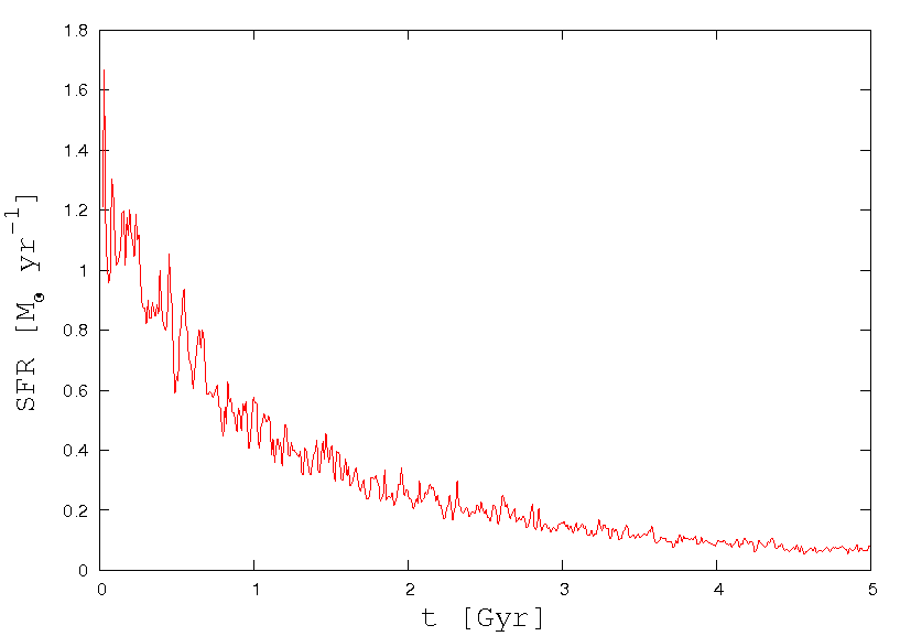
Figure 5.5: Star formation rate as a function of time for the MW model.

5.2.2 Global properties of the gas particles

Immediately after the entrance in MUPPI, i.e. when gas particles fulfills both the thresholds in density $n_{thr}$ and in temperature $T_{thr}$ (see Tab. 5.4), thermally unstable gas in the disk and in the bulge collapses, feeding the cold phase and thus causing a large burst of star formation. Such a burst is due to the sudden turning on of cooling and star formation physics. After about 2 Gyr, the MW galaxy settles down in a quiescent, self-regulated state with a star formation rate of nearly 0.2 $M_{\odot}$ yr^-1, as can be seen in Fig. 5.5. The SFR then slowly decreases as the cold gas is consumed by star formation. From the SFR plot, we thus deduce that MUPPI (with the parameters listed in Tab. 5.4) is able to lead to a self-regulated cycle of SF, where the growth of the cold phase and thus the star formation production are counterbalanced by the SNe feedback effects accounted in MUPPI (see Sec. LABEL:MUPPI:core).

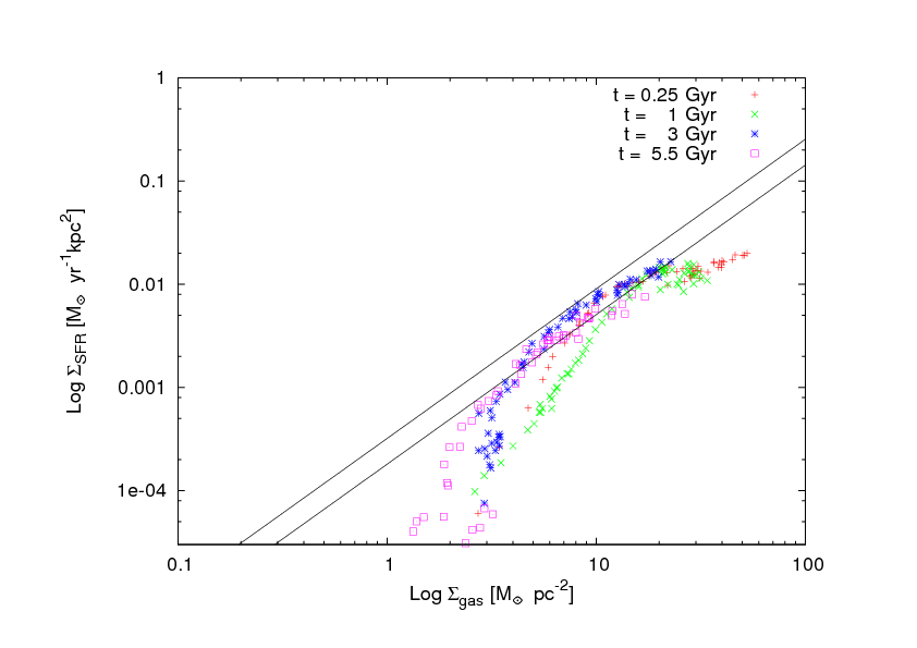
Figure 5.6: Star formation rate density as a function of cold gas surface density for the MW model. The solid lines mark the Schmidt-Kennicut law (1998).

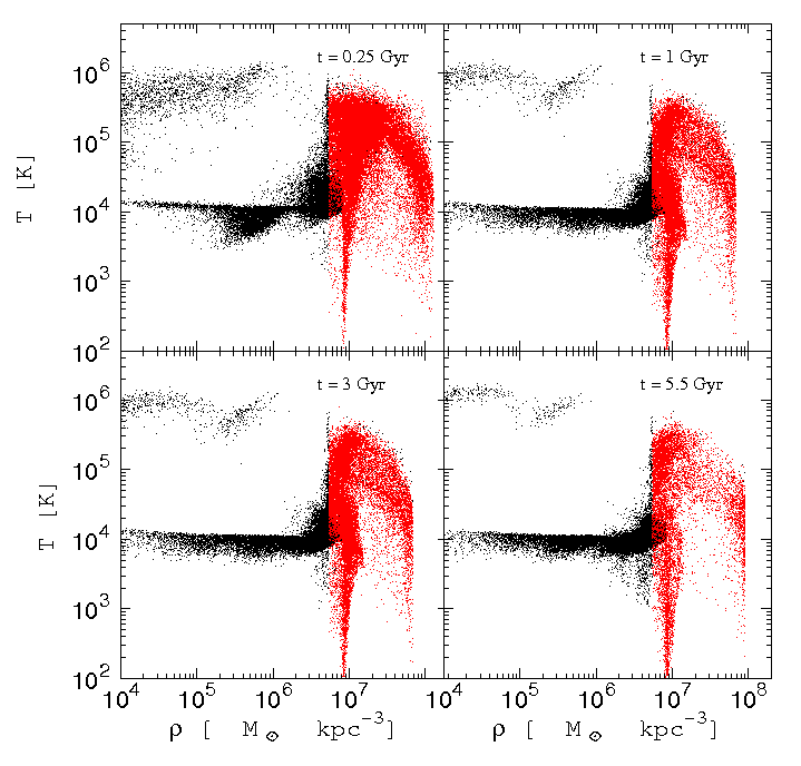
Figure 5.7: MW density-temperature phase diagram for SPH gas particle (black) and MUPPI gas particles (red). See text for details.

Observationally, the surface density of the star formation rate in different galaxies scales non-linearly with the surface density of the total gas. This relation is known as the Kennicutt-Schmidt star formation law: reproducing this relation in galaxy formation simulation is one of the main challenges for galaxy formation models. In Fig. 5.6 we plot the projected star formation rate density as a function of the cold gas surface density, at different times during the evolution of the MW galaxy model.

At the beginning of the simulation ($\approx$1 Gyr), the simulated Kennicut relation is slightly below the observed one, due to the high density reached in the galaxy centre after the prominent initial collapse. Then, the gas is consumed by star formation; in the meanwhile, runaway star formation is prevented by SNe energy feedback, which prevent too much hot gas to radiatively cool down to the cold phase. At later times, our simulated MW is in good agreement with the observed Schimdt-Kennicut (1998) relation, indicated on this plot by two solid lines: a further proof that MUPPI is able to generate a self-regulated ISM. The relation is reproduced at all times, up to the end of the simulation at 5.5 Gyr. Note that we are able to reproduce the star formation cut at low surface densities, while the GADGET effective model with kinetic feedback (i.e., winds) does not (see Fig. 5.14), as we shall see in the following section.

In Fig. 5.7 we show the SPH gas density vs average temperature phase diagram for the MW model at four times for the SPH gas particles (black) and the MUPPI gas particles (red). The diagram is populated in three main regions: gas lying on the disc is visible in a tight relation at $T$ = $10^{4}$ K; in the upper-left corner we see gas particles, once multi-phase, that have been driven outside the galaxy by the SNe feedback and that are now falling back to the galaxy while radiatively cooling. This is the typical behaviour of a galactic fountain. MUPPI gas particles, instead, occupy the dense region of the plot and take different temperatures, from $\sim$10² K to $\sim$5$\cdot 10^{5}$K. In the upper-left diagram (0.25 Gyr), at high densities and low temperatures, we see multi-phase particles which are cooling and probably will soon reach the conditions to spawn a star; note in fact how the number of multi-phase gas particles diminishes through time, due to the ongoing star formation which consumes the gas. Moreover, in the “multi-phase” region are evident gas particle which have been heated by SNe energy feedback but that are still in the multi-phase regime. In the four diagrams the density-temperature relation is sharply truncated at the density where the probability of spawning a star becomes nearly unity, i.e. beyond $\sim$9$\cdot$10⁷$M_{\odot}$kpc^-3.

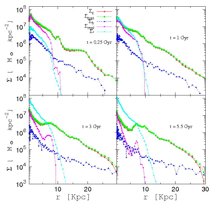
Figure 5.8: MW surface density profiles for stars ($\rho_{\star}$) and our various gas phases, i.e. cold ($\rho_{c}$), molecular ($\rho_{mol}$), hot ($\rho_{h}$)and total gas density ($\rho_{gas}$)

In Fig. 5.8, we show the radial surface density profiles for various components of the MUPPI gas particles at four different times. Here and in the following, we evaluated density profiles using 100 radial bins, equally spaced in $log(r)$, and ranging from 0.5 to 50 kpc. When galaxy models are concerned, we projected the particle positions on the disk plane to obtain surface density profiles. For the isolated halos cases, we instead used 3D radial density profiles. We weighted hot phase gas temperature and numerical density profiles by the hot phase gas mass; cold phase numerical temperature by the cold pase gas mass, and pressure by the total gas mass.

In general, the global behaviour of the gas particles reflect that of the single particles we described in the previous section. At $t$ = 0.25 Gyr (top left panel), the initial strong burst of star formation has just begun, thus the star density $\rho_{\star}$ is low and corrispondently the density of the cold $\rho_{c}$ and molecular phase $\rho_{mol}$ is high, reaching $\sim 3\cdot 10^{7}$ $M_{\odot}$ Kpc^-3. Going further in time, the cold gas phase (together with the molecular phase) slowly undergoes depletion due to star formation while the SN energy injected by the newly born stars rises the temperature of the hot phase thus making radiative cooling

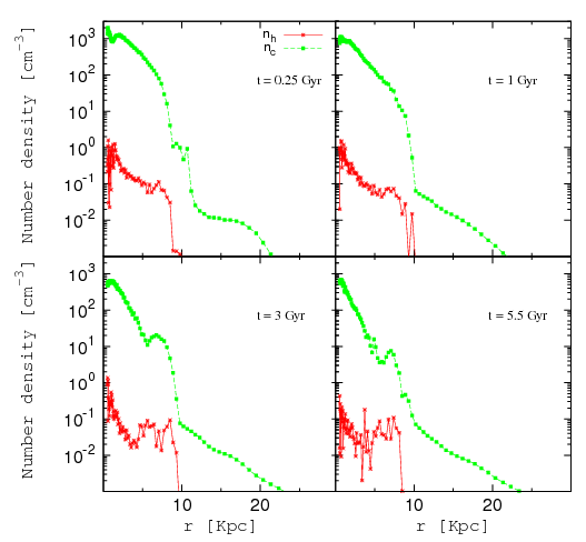
Figure 5.9: MW number density profiles for the cold phase (green) and the hot phase (red).

less efficient and limiting the cold phase replenishment. As observed in Milky Way-like galaxies, the surface gas density become exponential along the disc plane. The behaviour of the molecular phase (regulated by $f_{coll}$) is as expected: in the galaxy core, where the pressure is high, the gas at disposal for star formation is high, while this quantity diminishes while going further along the disc. The hot phase surface density follows the cold phase trend, but 2 orders of magnitudes below: in the core, where the star formation is high and thus is the SNe energy feedback, the gas is efficiently warmed up; towards the galaxy outskirts, the pressure declines leading to a lower star formation rate and thus a less efficient SN feedback injection. The density profile of the stellar mass, while increasing with time, slightly move outwards and, at 5.5 Gyr, extends till 15 Kpc. As shown in Fig. 5.12, MUPPI give rise to a thin stellar disk and to a stellar bulge.

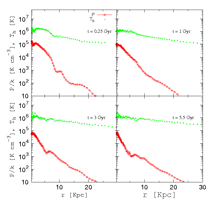
Figure 5.10: Hot temperature profiles (green) and gas pressure profiles for the MW simulation. See text for details.

In Fig. 5.9 we show the number density profiles for the hot and the cold phase at the the usual times. As expected from the surface density profiles described above, the cold number density is much higher than the hot one: it reaches its maximum value in the galaxy centre and rapidly declines till $\sim$ 12 Kpc (nearly the extension of the star forming region), where $n_{c}$ changes slopes and slowly declines along the disc ($n_{c}$ may be defined also for non multi-phase, cold gas). The presence of the bulge reflects in $n_{c}$ values well above $10^{2}$ at scales $r<5$ kpc. Note that at 8 Kpc from the MW centre (approximately the distance of the Sun from the Milky-Way centre), the cold number density value is between 10–100 cm^-3, in agreement with the observed values in the Solar System neighbourhood. For what concerns the hot number density, $n_{h}$ peaks in the centre at $\sim$ 1 cm^-3 and slowly declines till $\sim$ 10 Kpc beyond which $n_{h}$ sharply dimisishes.

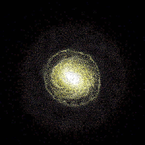
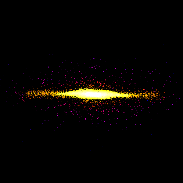
Figure 5.11: The distribution of gas in the xy plane (left panels) and in the xz plane (right panels) from the simulation of the MW galaxy, at 0.25, 1, 3 and 5.5 Gyr (from top to bottom). The frames are $60$ Kpc on a side. Colour scale is logarithmic and scales from $10^{-0.5}$ to $10^{5}$ times critical density.

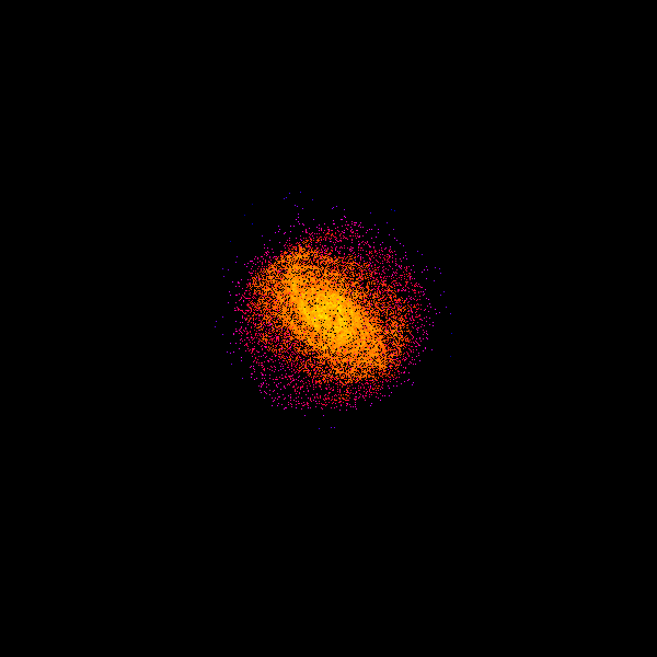
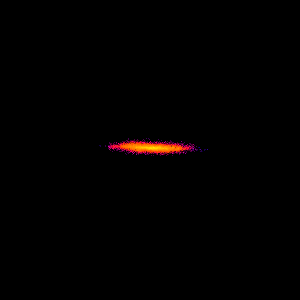
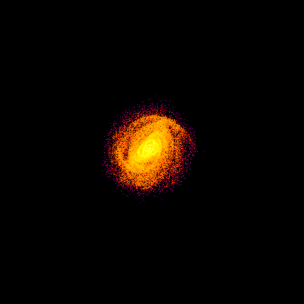
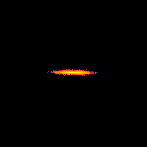
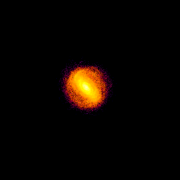
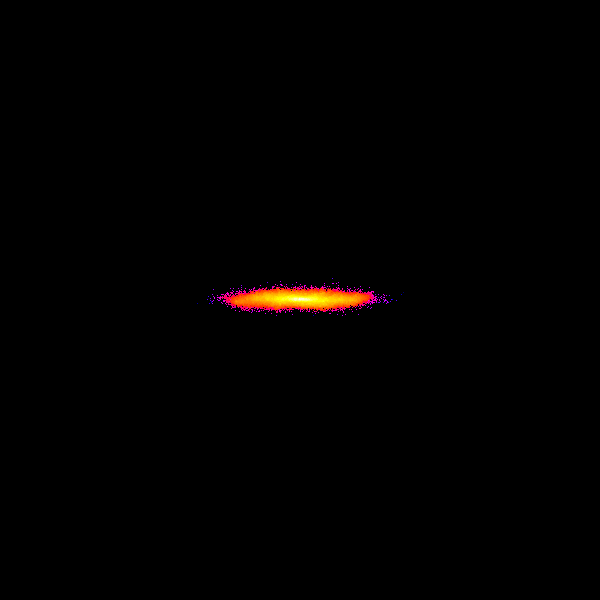
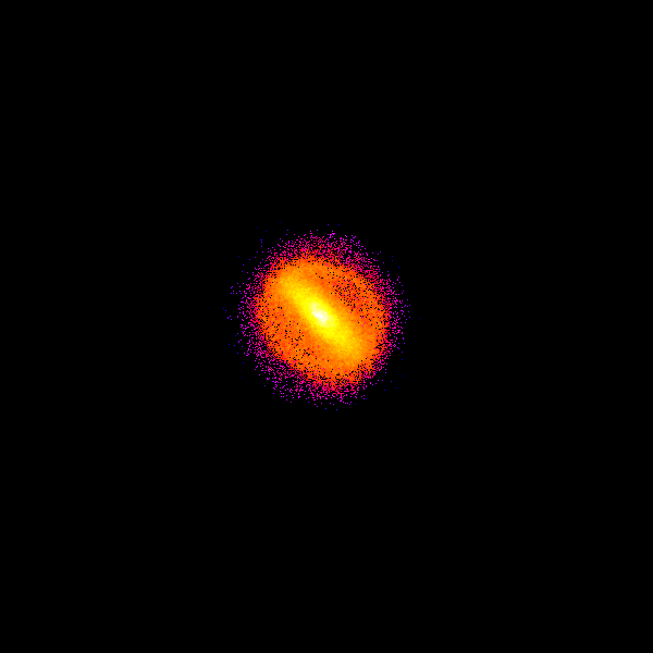
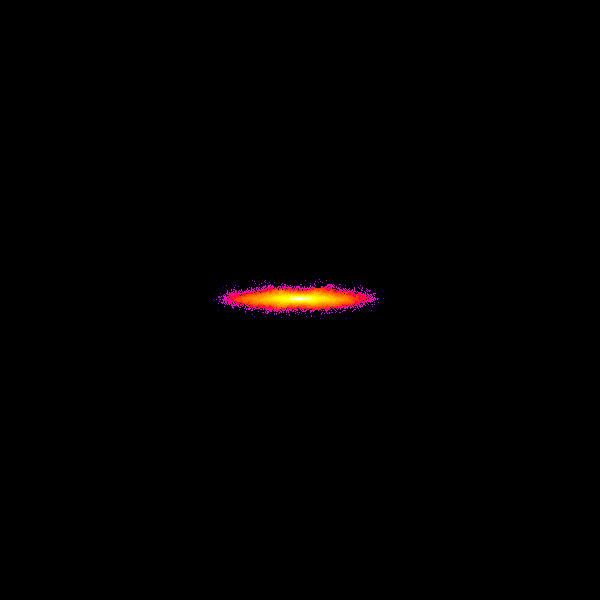
Figure 5.12: The distribution of stars in the xy plane (left panels) and in the xz plane (right panels) from the simulation of the MW galaxy, at 0.25, 1, 3 and 5.5 Gyr (from top to bottom). The frames are $60$ Kpc on a side. They show density maps generated with the SMOOTH algorithm, applied separately to the star particle distributions. Colour scale is logarithmic and scales from $10^{0.5}$ to $10^{7}$ times critical density.

The hot gas in our MW galaxy is almost isothermal with an average temperature of 10⁵–10⁶K, as shown in Fig. 5.10. In this figure we also plotted the total pressure of the SPH gas particles which, at variance with temperature, does vary depending on the position from the centre: while in the bulge the average pressure ranges between 10³–10⁵ K cm^-3, in the disc $P/K$ value is below $\sim$ 5$\cdot$10². Anyway, in the single particle plots (in Fig. 5.2– 5.3) we already noticed the gas isothermal behaviour (in fact, both core and disc particles has a $T_{h}\sim$10⁷) and the differences in pressure depending on the position from the galaxy centre.

5.2.3 Comparison with the GADGET effective model

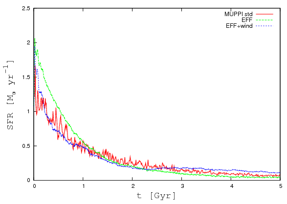
Figure 5.13: Star formation rate as a function of time for the MW model with MUPPI standard set of parameters (red solid line, see Tab. 5.4), and for the GADGET effective model with (blue short dashed line) and without (green dashed line) winds.

We performed a simulation of the MW model using the GADGET effective model (see Sec. 2.2.3) in order to compare MUPPI results (described in the previous section) with those obtained with the original GADGET star formation function.
In Fig. 5.13 we compare the star formation rates obtained simulating the MW model with MUPPI, the effective model(EFF) and the effective model with winds (EFF+W) having velocities equal to 340 km s^-1 (see Eq. 2.33). In all three schemes, star formation starts instantaneously because thermally unstable gas in the disk and in the bulge collapses becoming immediately star-forming. The behaviour of star formation in MUPPI and in EFF+W models is similar, with MUPPI star formation being more spiky then EFF+W. At the onset of the simulation, MUPPI and EFF+W have a SFR of $\approx$ 1.5 M_⊙ yr^-1 while EFF star formation rate is slightly more prominent being $\approx$ 2 M_⊙ yr^-1. After $\approx$ 1 Gyr, the three models converge to the same SFR, which then decreases with time. Note that at final times, the SFR trends are reversed with respect to the beginning: now the EFF+W SFR is slightly higher than EFF while MUPPI stays in the middle: this is due to the fact the higher the SFR the higher the velocity of gas consumption, and thus the faster the star formation is quenched due to the lack of gas supply.
As expected, the EFF model perfectly reproduce the Schmidt-Kennicut star formation relation, since here this relation is imposed by means of the star formation timescale (see Eq. LABEL:GDT:sf_timescale), as shown in Fig. 5.14. Introducing winds in the EFF model changes the results: now the EFF model is able to generate galactic fountains but in the meanwhile is no more able to reproduce the Schmidt-Kennicut law at low surface densities. As we have already discussed, MUPPI can generate galactic fountains and the Schmidt law even at low densities self-consistently (see Fig. 5.6).

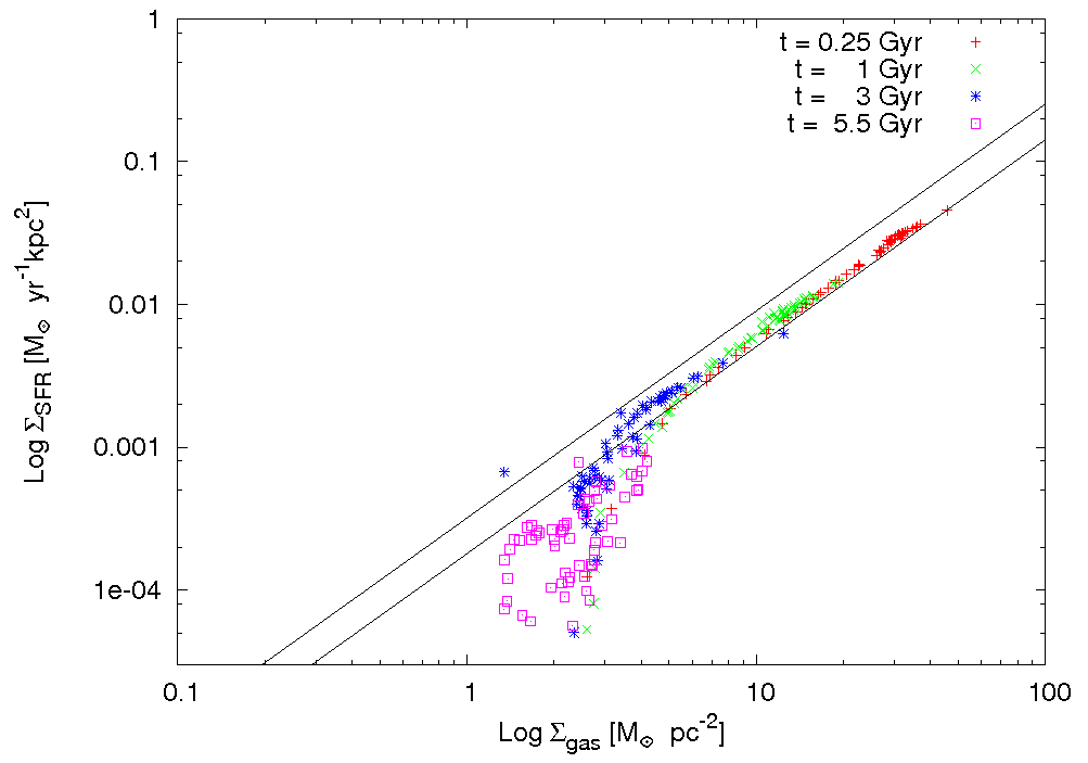
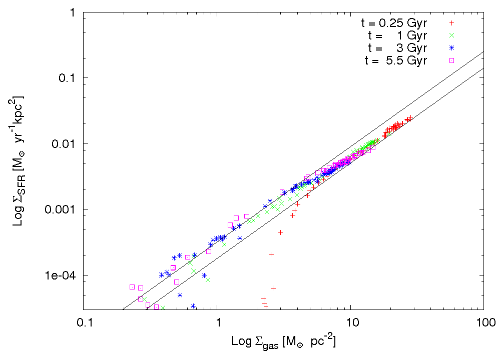
Figure 5.14: Star formation rate density as a function of gas surface density for the MW model with the effective model with winds (right panel) and without winds(left panel). The solid lines mark the Schmidt-Kennicut law (1998).

As a last comparison with the EFF model, we present in Fig. 5.15 the phase diagrams ($T$ vs $\rho$) of the MW with standard EFF star formation (i.e. no winds). We precedently described the same diagram obtained with MUPPI in the previous section. The EFF model phase diagram results drastically different from that of MUPPI (see Fig. 5.7): first of all, in the dense region of the plot, the gas particles follows a tight relation between $T$ and $\rho$, differently with MUPPI gas particles which instead show a larger variety of temperatures corresponding to the density.

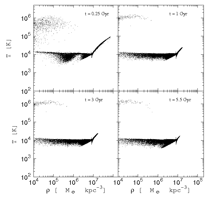
Figure 5.15: Density-temperature phase diagram for gas particle for the MW with the effective model without winds. See text for details.

5.2.4 Varying the blow-out efficiency

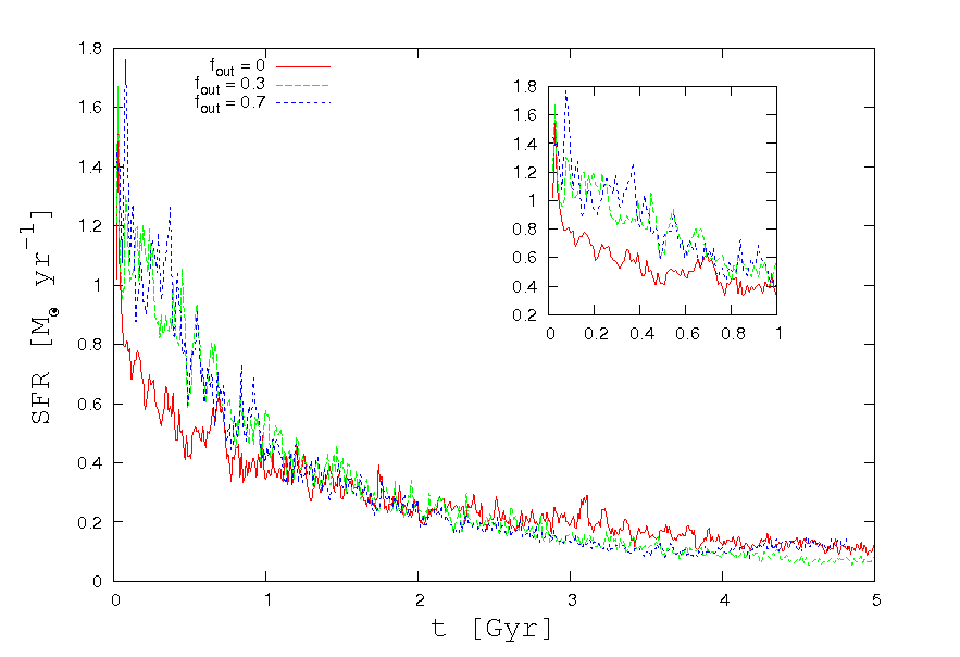
Figure 5.16: Star formation rate as a function of time for the MW model with varying fraction of SNe energy assigned to neighbouring particles. In the insert we focus the plot on the SFR till 1 Gyr since the onset of the situation. See text for details.

The effect of changing the fraction $f_{fb_{0}}$ of the SNe energy that blows outside the gas particle in the SFRs is demonstrated in Fig. 5.16. While the SFR follows the same general trend when increasing $f_{fb_{0}}$ from 0.3 (FB03) to 0.7 (FB07), in the case of zero blow-out efficiency (FB00) the SFR is slightly different. In fact, MUPPI star formation is driven by pressure. Within each MUPPI particle, SNe energy pressurises the hot phase. Part of such energy is provided by SNe exploding inside the particle, but another part comes from neighbouring multi-phase particles. When we set $f_{fb_{0}}=0$, this source of pressurisation is not present and as a consequence, the star formation proceeds much slower.

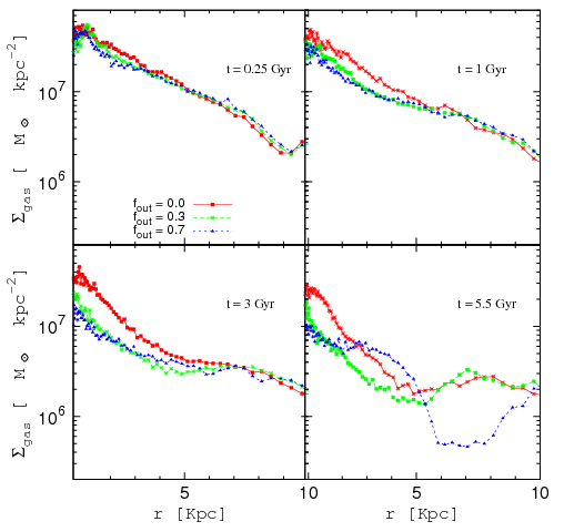
Figure 5.17: Surface density profiles for the MW model with $f_{\rm fb,o}=0.$, $0.3$, $0.7$ for stars ($\rho_{\star}$) and different gas phases, i.e. cold ($\rho_{c}$), molecular ($\rho_{mol}$), hot ($\rho_{h}$) and total gas density ($\rho_{gas}$)

As we can see from Fig. 5.16, runs with non-zero blow-out fraction have an higher star formation efficiency and thus consume much faster the gas supply. At final times the, the trends are reversed with the FB00 run having a larger reservoir of gas to convert in stars than the other two cases. This difference in gas supply between the three runs is confirmed in Fig. 5.17 where we show the surface density profiles at the usual times. If at 0.25 Gyr the profiles are very similar, their behaviour changes with time, with the “blow-out” runs being less dense in the first $\approx$ 8 Kpc from the centre than the FB00 simulation. Note that at 5.5 Gyr the FB07 run shows a density drop between 5 and 10 Kpc, due to the onset of an instability leading to the formation of a very strong bar. Apart the strong bar formation, there is not such a difference at this level in choosing $f_{fb_{0}}$ to be 0.3 or 0.7. Anyway, if one plots the density-star formation rate relationship for the FB07 case as shown in

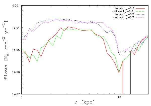
Figure 5.18: Inflow and outflow star rates for the MW model with $f_{\rm fb,o}$ = 0.3 and $f_{\rm fb,o}$ = 0.7.

We also evaluated gas outflows and inflows generated by the hot gas particles heated by SNe energy and floating away from the disk plane. To do this, we calculated how many gas particles lie in a slice with z coordinates $-2<z-1$ kpc and $1<z<2$ kpc. We assign to “outflows” those gas mass particles having negative velocities when z¡0 and positive velocities when z¿0, and to “inflows” the gas particles having opposite behaviour. In Fig. 5.18 we show the resulting mass outflow and inflow as a function of the distance from the centre of the disk for both cases FB03 and FB07. Outflows and inflows have very similar values, being higher for FB07 as expected. This is a tipi-Cal signature of galactic fountains, with heated gas floating away but not escaping, cooling and falling again on the disk.

Fig. 5.19, an important difference with the FB03 run rises: in fact, in FB07 we reproduce the observed Schmidt-Kennicut law worser than in FB03, being the cut at low surface densities too high with respect to observations. This is the main motivation why we have chosen $f_{fb_{0}}$ = 0.3 to be our reference value for modulating the blow-out energy.

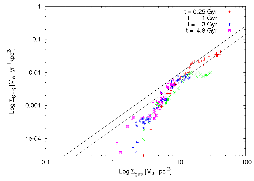
Figure 5.19: Star formation rate density as a function of gas surface density for the MW with $f_{\rm fb,o}$ = 0.7. The solid lines mark the Schmidt-Kennicut law (1998).

5.3 Other cases

5.3.1 Dwarf galaxy

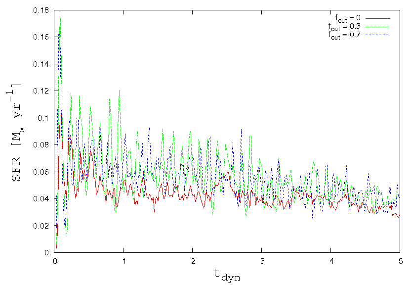
Figure 5.20: Star formation rate as a function of time for the DW model with $f_{\rm fb,o}=0$, $0.3$ and $0.7$. See text for details.

We run a set of simulations with the purpose of assessing how MUPPI behaves on different initial physical conditions. All the numerical parameters of the simulations are the same as in the MW case, except mass resolution and softenings (see Tab. 5.2).

Here we show our results for the DW run. As we did for the MW one, we investigate the SFR history and compare results obtained varying the blowing-out SN energy, as shown in Fig. 5.20. As expected, the SFRs are lower than in the MW run, being the DW galaxy less massive and dense, and thus less pressurised. Again, the FB00 run has the lowest SFR while the FB03 and FB07 show a similar behaviour, with a higher SFR. As in the MW then, turning off the blow-out regime lead to a low pressure ISM and a corresponding low star formation efficiency: the fact the ISM is less pressurised also causes the fraction $f_{coll}$ of molecular gas to decrease. This is similar to what happens at the edges of the MW disk (see Fig. 5.8), and is shown in Fig. 5.21.

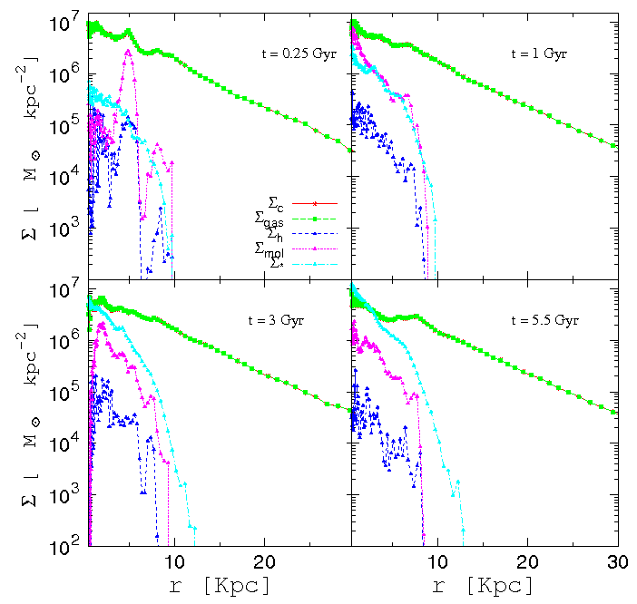
Figure 5.21: DW surface density profiles for stars ($\rho_{\star}$) and different gas phases, i.e. cold ($\rho_{c}$), molecular ($\rho_{mol}$), hot ($\rho_{h}$)and total gas density ($\rho_{gas}$)

Here we show for the FB03 run gas surface density profiles for cold and hot phase, stars, molecular phase and the whole gas; the molecular density profile $\Sigma_{mol}$ evolution is shown as purple lines with triangles. In this case, the amount of molecular gas is always a relatively small fraction of the cold gas, while in the MW case the molecular gas fraction was almost unity in the centre and declined towards the edge of the star forming zone (see Fig. 5.8).

From Fig. 5.21, we see that the DW interplay among different phases and the resulting self-regulated regime is very similar to that found in the MW case, even if all surface densities reach lower values, due to the shallower gravitational potential well produced by the halo in this case.

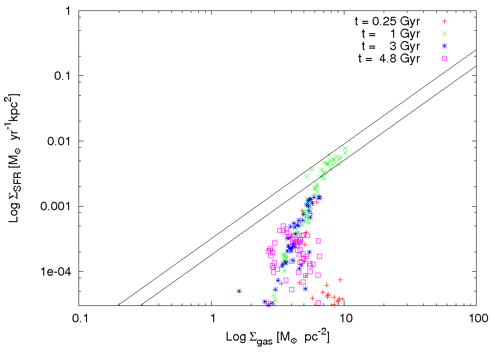
Figure 5.22: Star formation rate density as a function of gas surface density for the DW model. The solid lines mark the Schmidt-Kennicut law (1998).

The density-SFR relation for the FB03 DW galaxy does reproduce only the declining part of the Schmidt-Kennicut relation (see Fig. 5.22); in this case, cold gas surface density high enough to be significantly compared with local observation are only occasionally reached.

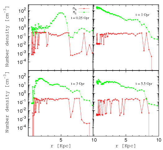
Figure 5.23: DW number density profiles for the cold phase (green) and the hot phase (red).

In order to complete the comparison with the MW galaxy we show in Fig. 5.23 and in Fig. 5.24 the number density profiles and the pressure-temperature evolution. The number density profiles follow very closely the behaviour of the surface density profiles, discussed above and showed in Fig. 5.8. At 0.25 Gyr, a large fluctuation in $n_{c}$ is visible around 5 Kpc from the centre: this bump likely originates due to the initial large burst of star formation which generates a pressure wave propagating through the galaxy disk. This pressure wave is clearly visible from the pressure plot in Fig. 5.24. In the top-left panel of Fig. 5.25 the pressure wave instability generates a ring-like structure around the galaxy centre which disappears later on. This behaviour is caused by the sudden turn-on of cooling and star formation physics and should be regarded as a numerical effect.

As in the MW, the hot gas in our DW galaxy is almost isothermal with an average temperature oscillating between some 10⁵ to 10⁶ K, as shown in Fig. 5.24. The reason why the temperature profile is sharply interrupted is that beyond 10 Kpc there are not multi-phase gas particles. This does not happen to the pressure trend because pressure can be estimated on all the SPH particle.
All the ISM properties we showed in this section closely resemble our result for the MW disk, far from its bulge. Overall, the simulations of the DW galaxy, correctly reproduce the general properties expected for a quiet lighter galaxy, with a less active ISM.

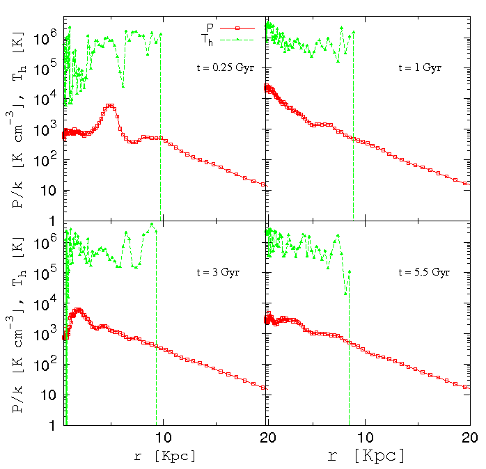
Figure 5.24: Gas pressure profile (red) and temperature profile (green) of the hot phase for the DW galaxy model.

Comparing the distribution of gas at various times for the MW and DW disk (figs…), a difference appears. In the MW case, the gas disk develops long lasting, sharp spiral arms (xy view) and part of the gas is expelled from the disk, and then falls back in fountains (xz view). In the DW case, such an outflow is almost unappreciable, and the xy view shows a more irregular, disturbed structure.

This is due to the difference in the feedback strength. The high pressure, and thus high SFR level and energy feedback, present in the MW, heats the hot phase enough to drive gas particles outside the disk, forming a “thermal wind”. Such particles bring energy away from the plane, then cool down, after exiting the multi-phase stage, and can thus originate fountains.

The pressure in the DW case is not high enough for this to happen; on the other hand, hot gas in the disk still exerts hydrodynamical pressure on neighbours, destabilising the disk structure and carving cavities (resembling SNe super-bubbles) in it.

Figure 5.25: The distribution of gas in the xy plane (left panels) and in the xz plane (right panels) from the simulation of the DW galaxy, at 0.25, 1, 3 and 5.5 Gyr (from top to bottom). The frames are $80$ Kpc on a side. Colour scale is logarithmic and scales from $10^{-0.5}$ to $10^{5}$ times critical density.

Figure 5.26: The distribution of stars in the xy plane (left panels) and in the xz plane (right panels) from the simulation of the DW galaxy, at 0.25, 1, 3 and 5.5 Gyr (from top to bottom). The frames are $80$ Kpc on a side. They show density maps generated with the SMOOTH algorithm, applied separately to the star particle distributions. Colour scale is logarithmic and scales from $10^{0.5}$ to $10^{7}$ times critical density.

5.3.2 Isolated non-rotating haloes

In this section, we describe simulations of isolated non-rotating haloes described in Sec. 5.1.1, evolved using MUPPI.

CFDW

In Fig. 5.27 we show the SFRs obtained by for the CFDW halo varying the fraction of SNe energy blowing out of the gas particle ($f_{\rm fb,o}$ = 0.0, 0.3,0.7) in the MUPPI code. For comparison we also show the SFRs for the GADGET effective model (EFF) and the effective model with winds (EFF+wind). In all runs, star formation starts few Myrs after the onset of the simulation, when the cooling flow is established and core gas is dense and cold enough to fulfil star formation thresholds.

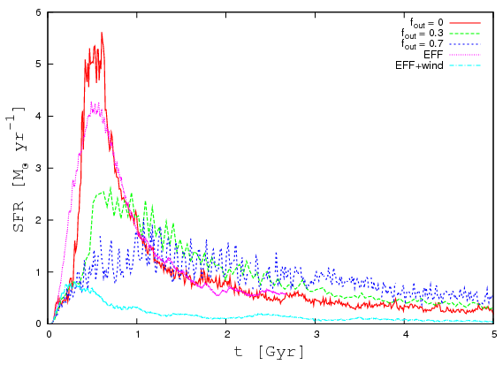
Figure 5.27: Star formation rate as a function of time for the CFDW model simulated with MUPPI, with $f_{\rm fb,o}$ = 0.0; 0.3;0.7 and, for comparison, with the GADGET effective model without winds (EFF) and with winds (EFF+wind). See text for details.

The behaviour of star formation when using MUPPI is reversed, with respect to

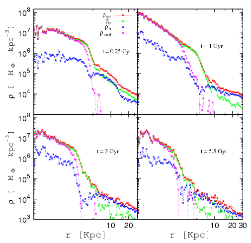
Figure 5.28: CFDW density profiles for cold ($\rho_{c}$), molecular ($\rho_{mol}$), hot ($\rho_{h}$)and total gas density ($\rho_{gas}$).

the results already obtained for the galaxy cases: the more the energy blowing out the multi-phase gas particles, the more the cooling flow is quenched as thus the star formation suppressed. The FB00 run has a large burst of star formation at $\sim$ 0.7 Gyr, leading to a SFR of $\sim$ 5 M_⊙ yr^-1 which, due to gas consumption, rapidly decreases with time. Note that the SFR history of our FB00 model is very similar to that obtained using SH03 effective model without kinetic feedback. In the FB03 and FB07 runs the bursts of star formation are less intense than in the FB00 case. The SFR peak is reduced of a factor $\approx$ 2.5 using FB03 and a factor $\approx 5$ using FB07. Thus, the feedback energy injected in the medium is thus very efficient in countering the cooling flow. As already noted in the “galaxy” tests, these trends are reversed at final times: at 5 Gyr, the FB07 SFR is

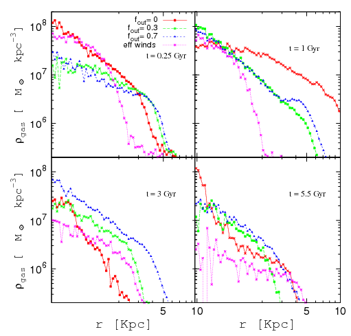
Figure 5.29: Density profiles for the CFDW model with varying fraction of blowing SNe energy for cold ($\rho_{c}$), molecular ($\rho_{mol}$), hot ($\rho_{h}$)and total gas density ($\rho_{gas}$).

slightly higher than FB00 and FB03, being larger the amount of gas which has not yet been converted in stars.
Note adding kinetic winds to the EFF model drastically reduces the efficiency of star formation at all times. The reason for the low EFF+wind SFR is that here the winds are very effective in ejecting gas particles outside shallow potential well of this small halo. Applying the wind scheme to such a low mass halo simply clears it of its gas content, while “thermal” winds generated self-consistently by MUPPI do allow sustained star formation, if at a low rate, till the end of the simulation.
In Fig. 5.28 we show the multi-phase gas particles density profiles at the same times already shown in previous cases, for the FB03 model.

CFMW

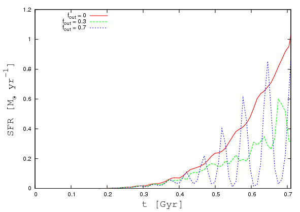
Figure 5.30: Star formation rate as a function of time for the CFMW model simulated with MUPPI, varying $f_{\rm fb,o}$ = 0.0; 0.3;0.7 and, for comparison, with the GADGET effective model without winds (EFF) and with winds (EFF+wind). See text for details.

The general behaviour for the different gas components (i.e. cold, molecular, hot) is that already found in the “galaxy” models, with cold and molecular gas growing in the halo core where a high pressure is reached and hot phase increasing due to the SN feedback injection. The fraction of molecular gas, in particular, resembles what we found for the MW bulge and it is always of order unity up to the edge of the star-forming, multi-phase region. Note how all gas densities grow between 0.25 Gyr and 1 Gyr: in this interval of time, a strong cooling flow is established which feeds the cold and molecular phase, thus igniting a burst of star formation which pressurises the whole region. At 3 Gyr, most of the gas previously collapsed in the galaxy core has been already converted into stars. Since then on, the density profiles of the various gas phases stay approximately constant, in a self-regulated fashion. Also, comparing density profiles of hot and cold gas phases with those obtained in the galaxy runs, we can see that a larger fraction of gas is in the hot phase, similarly to what happens in the bulge of our MW run, while such fraction is much lower in MW disk and in the DW run. This is due to the fact that, in this configuration, external pressure of infalling gas forbids a larger fraction of hot, multi-phase particle to escape the star forming region via buoyancy. More SNe energy thus remains in the zone, and heats a larger amount of gas away from the cold phase. At the same time, each multi-phase gas particle has a higher amount of hot gas and less gas in the cold phase; this is the reason why the trend of SFR with $f_{\rm fb,o}$ is reversed.

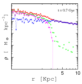
Figure 5.31: CFMW density profiles for ($\rho_{c}$), molecular ($\rho_{mol}$), hot ($\rho_{h}$) and total gas density ($\rho_{gas}$).

In Fig. 5.29 we can further appreciate the efficiency of thermal feedback in MUPPI for the CFDW case and its dependency on the amount of energy transferred outside the multi-phase gas particles to their neighbours. Here we show the total gas density profiles for FB00, FB03, FB07 and EFF+wind runs at four different times. FB00 quickly consumes a large amount of gas, its density profile decreases and gets steeper. The larger the energy given to neighbouring particles, the smaller is the gas consumption, and also the slope of the profile is shallower.

Due to the high cost in computational time, the simulations runs of the CFMW halo has been evolved just till $0.7$ Gyr.
In Fig. 5.30 we present the SFRs obtained by varying the SNe energy blowing out efficiency: the general behaviour is similar to that already found for the CFDW case. The FB07 SFR is intermittent and spiky, because many gas particles reach the conditions for entering the multi-phase star formation regime at the same time and in a high pressure environment, and thus a huge fraction of SN energy feedback is injected in the medium simultaneously, depressing the SFR. When this heated gas cools and condenses, fulfils again the thresholds and the cycle is repeated. We already found a similar behaviour in the simulations ran with an implementation of the Stinson et al. 2006 star formation and feedback scheme, which uses the Thacker $\&$ Couchman (2000) feedback (see Sec. 2.5.3); the difference is that MUPPI is able to “stop” radiative cooling self-consistently, without any ad-hoc artificial assumptions as instead the Stinson 2006 recipe does. However, this spiky SFR behaviour is almost not present when lower fraction of energy are ejected to neighbouring particle.

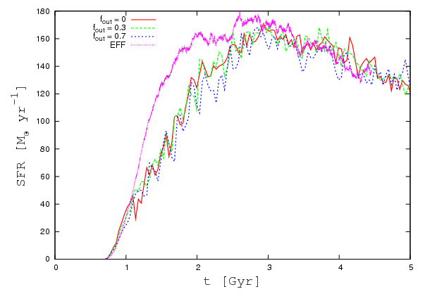
Figure 5.32: Star formation rate as a function of time for the Me13 model simulated with MUPPI, varying $f_{\rm fb,o}$ = 0.0; 0.3;0.7, and, for comparison, with the GADGET effective model without winds (EFF).

As in Fig. 5.28, in Fig. 5.31 we show the density profiles for the different gas components considered in MUPPI. We show here the latest time of out CFWM run only. Here, the star forming zone, where the cold gas phase is dominant and the molecular fraction is high, is confined to the very inner regions of the halo, near to the softening length. But the pressure exerted by infalling, cooling gas is large enough to trap almost all the multi-phase particles heated by the SNe energy feedback. As a consequence, in the centre of the halo a large fraction of the gas is in the hot phase. Such hot gas exerts enough pressure to counter that of the infalling gas: it is again an example of the efficiency of thermal feedback we obtain with MUPPI as far as this mass scales are concerned.

We also run our Me13 cooling-flow halo (See Cap. 2) using MUPPI with our standard parameter set and varying $f_{\rm fb,o}$. In Fig. 5.32 we show the star formation history for cases FB00, FB03, FB07 and for the EFF model already show in Cap. 2. In this case, the effect of increasing the SNe energy fraction transferred to neighbouring particle is not strong. We can appreciate a decrease in the star formation rate at its onset, between 1 and 3 Gyr, with respect to the EFF model case. However, gas density profiles (not shown) are similar for all of such four runs. At this mass scales, SNe energy feedback is not very effective in countering the cooling flow even when MUPPI is used. The general ISM properties we obtain in the Me13 case are similar to those shown for the CFMW one.

5.4 Parameter tests

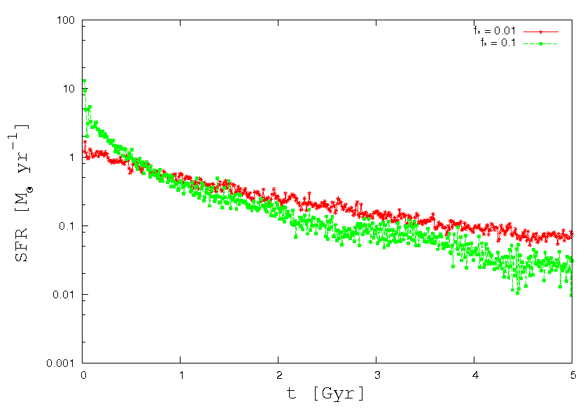
Figure 5.33: Star formation rate as a function of time for the MW model with our reference star formation efficiency $f_{\star}$ = 0.01 and with $f_{\star}$ = 0.1. See text for details.

In order to assess the response of the MW and DW galaxies to the adopted MUPPI parameters we ran a set of simulations varying three of the ten free parameters itemised in Tab. 5.4, i.e. $f_{\star}$, $f_{\rm fb,i}$, $n_{thr}$. We already studied the effect of having different values for $f_{\rm fb,i}$. We set the remaining parameters on the basis of the work of M04, on which our model is based.

When we vary one of such parameters, we keep constant all the remaining ones to their standard values. We first discuss the additional tests done on the MW galaxy. The effect of increasing the star formation efficiency $f_{\star}$ by one order of magnitude (from 0.01 to 0.1) is as expected. In Fig. 5.33 we compare the SFRs obtained by varying $f_{\star}$: at the onset of the simulation, the $f_{\star}$0.1 run is more efficient in forming stars, but at final times, the SF efficiency decreases due to greater consumption of gas if compared to the reference $f_{\star}$ run (i.e. 0.01). In Fig. 5.34 we moreover show the density-SFR relation in the $f_{\star}$0.1 case: the star formation is much more efficient than is observed after 0.25 Gyr since the onset of the simulation; thus the gas supply is consumed rapidly and the density-SFR relation is no more able to satisfy the Schmidt-Kennicut law, forming too many stars at any given surface gas density. Thus, for MUPPI low values of this parameters have to be preferred.

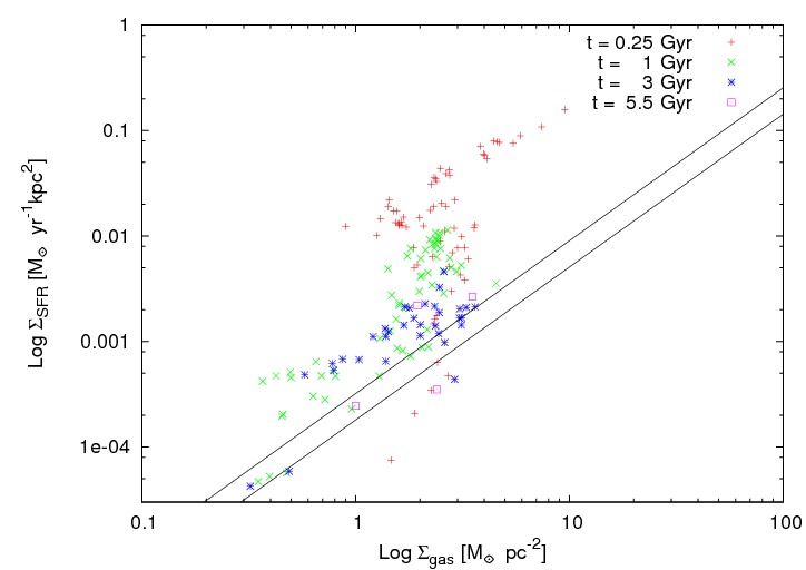
Figure 5.34: Star formation rate density as a function of gas surface density for the MW model with $f_{\star}$ = 0.1. The solid lines mark the Schmidt-Kennicut law (1998).

The last test we performed on the MW galaxy deals with the SN feedback energy. We tested the effect of increasing the fraction $f_{\rm fb,i}$ of SN energy which remains trapped inside the star forming gas particle rather than being ejected outside the gas particle. Note that the the two parameters $f_{\rm fb,i}$, $f_{\rm fb,o}$ are not related, the only requirement being that their sum must be lesser than unity. We consider the SNe energy not accounted for by the sum of $f_{\rm fb,i}$ and $f_{\rm fb,o}$ to be radiated away and lost as far as the ISM is concerned. In Fig. 5.35 we show the density-SFR relation obtained from a simulation where we set $f_{\rm fb,i}=0.05$ (reference value is 0.02). The plot shows that we don’t reproduce the Schmidt-Kennicut law as well as in the reference simulation (see Fig. 5.6). Our SFR at any given cold gas surface density is now lower than observed. Since the SF history has no appreciable differences from the case $f_{\rm fb,i}=0.02$, we deduce that coupling more SNe energy to the ISM inside the particle pressurises it more, giving a higher hot gas phase fraction and a smaller SFR. We thus prefer our reference value $f_{\rm fb,i}=0.05$.

Notice that increasing the star formation efficiency parameter and increasing the amount of energy coupled to the particle ISM modify our Kennicut relation in opposite directions. However, this does not obviously translate in the possibility to vary such two parameters in opposite direction while keeping the star formation history and the resulting Kennicut relation unchanged. E.g., a test run with $f_{\rm fb,i}=0.05$ and $f_{\star}=0.05$ could not give a Kennicut relation in agreement with observations. This is due to the non-linear behaviour of our model, which couples the effect of varying the parameters in a non-straightforward way.

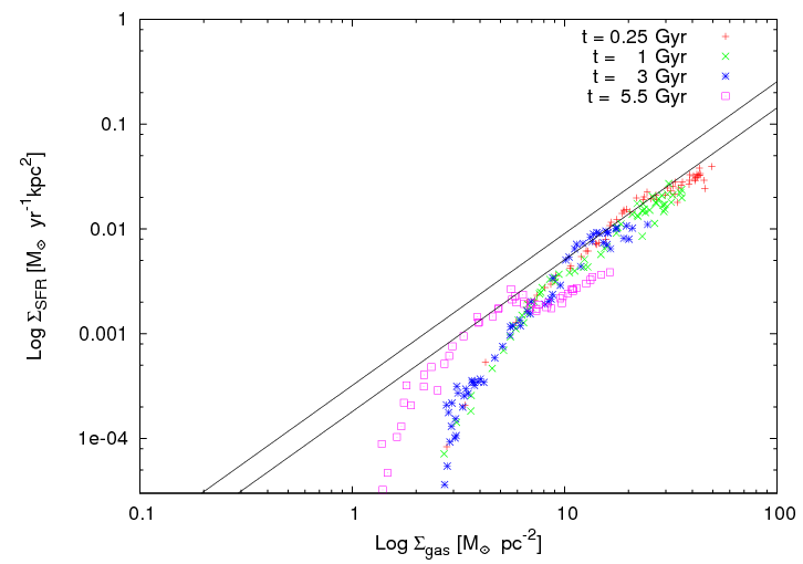
Figure 5.35: Star formation rate density as a function of gas surface density for the MW model with $f_{\rm fb,i}$ = 0.05. The solid lines mark the Schmidt-Kennicut law (1998).

We now discuss an additional test done on the DW galaxy. An important factor in star formation models is the density threshold at which star formation starts. In MUPPI, such a threshold regulate the initial particle pressure, and the degree of activity of the ISM and the duration of the multi-phase stage. In fact, the lower the initial pressure is, the more “quiet” the behaviour of the ISM and the longer the initial cold phase dynamical time are. We thus ran two additional simulations decreasing the number density threshold $n_{thr}$ from 0.25 cm^-3 to 0.1 and 0.05 cm^-3.

Figure 5.36: Star formation rate as a function of time for the DW model with varying threshold number density for entering the multi-phase state. We resample the SFRs with a constant time interval equal to $\sim$ 0.03 t${}_{d}yn$. See text for details.

In Fig. 5.36 we show the resulting SFR histories: the reference SFR (with $n_{thr}$ from 0.25 cm^-3) is initially the highest. This is simply explained by considering that increasing the density threshold, the central star forming region is smaller and thus need more time to accrete gas from the surroundings. After such a transient period, the SFR is very similar for the three different thresholds; in this regard, MUPPI shows to be quite insensitive to it. Fig. 5.38 shows the total gas surface density for our three different thresholds at four different times. Even the surface density profiles does not substantially vary when the density threshold for the onset of multi-phase regime is changed.

As we already show in Sec. 5.3.1, the cold gas density in the DW case is never high enough to sample the power-law part of the Schmidt-Kennicut law, and also with our standard parameter set, we only reproduce its low-density decline. However, we show in Fig. 5.37 surface density-SFR relation we obtain when varying the density threshold. A slight trend to get a lower SFR at given density for lower threshold values can be seen. This is related with the slower “metabolism” of multi-phase particles when their initial pressure is lower. The trend is not clear enough to give clear indication on the best value for this parameter; we selected as our default the one most used in the literature, and also selected by the SH03 star formation scheme.

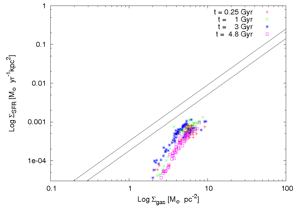
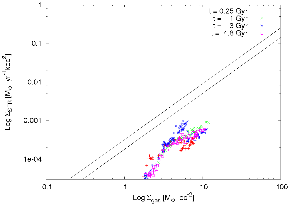
Figure 5.37: Star formation rate density as a function of gas surface density for the DW model with $n_{thr}$ = 0.1 cm^-3 (left panel) and $n_{thr}$ = 0.05 cm^-3 (right panel). The solid lines mark the Schmidt-Kennicut law (1998).

Figure 5.38: Surface density profiles for the MW model with different number density threshold $n_{thr}$, for stars ($\rho_{\star}$) and different gas phases, i.e. cold ($\rho_{c}$), molecular ($\rho_{mol}$), hot ($\rho_{h}$)and total gas density ($\rho_{gas}$)

5.5 Numerical tests

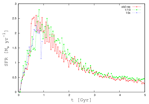
Figure 5.39: Star formation rate as a function of time for the CFDW model at standard resolution (std), low resolution (1/10) and high resolution (10x), using the reference set of MUPPI parameters. We resampled the SFRs with a constant time interval equal to $\sim$ 0.01 t${}_{d}yn$.

Finally, it is important to test how much the results presented in this Chapter depend on the numerical resolution of the simulations. To this aim, we carried out one simulation with the MW galaxy decreasing the number of gas and dark matter particles by a factor of ten (LR). Moreover, we performed two simulations of the CFDW halo in HR and LR. We run all the resolution tests with our reference set of MUPPI parameters (see Tab. 5.4).

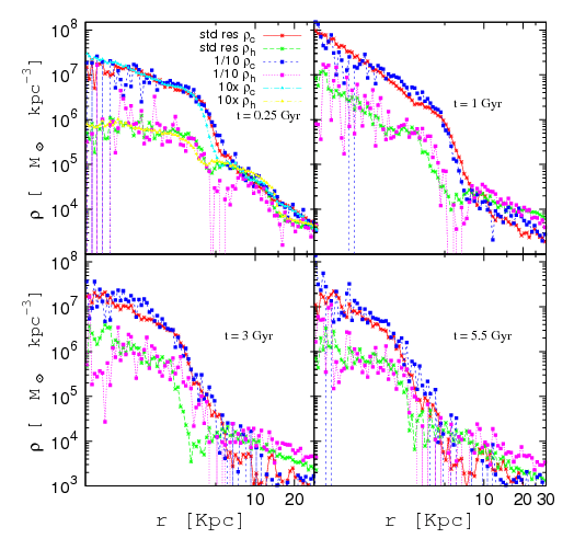
Figure 5.40: CFDW density profiles for the cold and the hot phases at standard resolution (std res), low resolution (1/10) and high resolution (10x).

In Fig. 5.39 we show the evolution of the SFR obtained with standard, low and high resolution for the CFDW halo. We evolved the HR run just till 1 Gyr due to the high cost in computational time. From this figure we can see that resulting SFR history does not show significant differences when the resolution is varied of a factor 100.

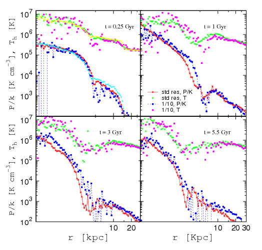
Figure 5.41: CFDW pressure and hot temperature profiles at standard resolution (std res), low resolution (1/10) and high resolution (10x).

To further probe the stability of our ISM model with varying resolution, we plot in Fig. 5.40 the radial density profiles of both the hot and cold phase. The three different resolution simulations once again behave in a very similar way. The only appreciable difference is that scatter in the profiles reduces with increasing resolution: the HR simulations are in fact described with a greater number of particles and thus have a much larger covering factor. This trend is confirmed in Fig. 5.41, where we plot pressure and temperature radial profiles: results at different resolutions are well convergent, thus confirming the numerical stability of our code when we change resolution by two order of magnitude for this halo.

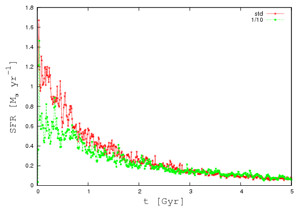
Figure 5.42: Star formation rate as a function of time for the MW model at standard resolution (res) and at low resolution (1/10), using the reference set of MUPPI parameters. See text for details.

For what concerns the MW galaxy, we present in Fig. 5.42 a comparison of the SFRs obtained at standard ($\rm std$) and low resolution ($\rm 1/10$). This numerical resolution test is quite different from the CFDW one. In the latter, gas is initially in hydrostatic equilibrium with the DM gravitational potential; in the core, temperature, density and pressure initial profiles are quite flat. Thus, varying the resolution influences how the physical quantities are sampled, but does not change their average value per particle. In the MW case, instead, we have an exponential surface density profile. Thus, under-sampling the gas particle distribution also means assigning lower density to low resolution gas particles at the same distance from the disk centre of the corresponding particles in high resolution case.

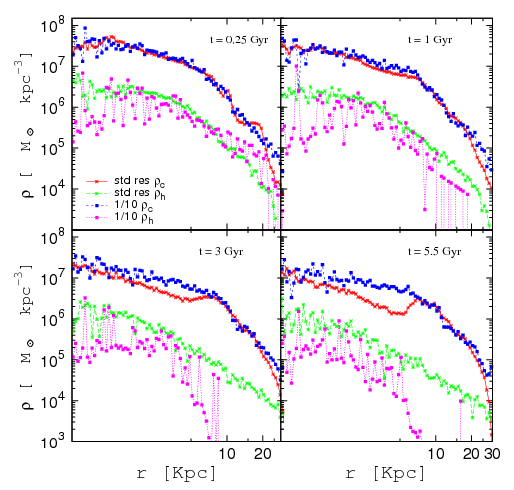
Figure 5.43: MW density profiles for the cold and the hot phases at standard resolution (std res) and low resolution (1/10).

At the onset of the simulation, the star formation activity is stronger in the $\rm std$ run, since a larger amount of gas cools here than in the lower resolution run. This implies that more gas particles fulfils the multi-phase regime thresholds and as a consequence the star formation efficiency is increased. This effect is given by the fact that gas particles in our standard resolution run reach higher densities, and cooling can begin before; it is not related to the star formation model. After less than 1 Gyr, the two star formation histories do converge to similar values and becomes identical after $\approx 2$ Gyr.

In Fig, 5.43 we show the cold and hot gas surface density profiles for our standard and LR runs. While the cold phase is extremely stable against varying the numerical resolution, the hot phase surface density show a clear decrease when resolution is lowered. A similar effect is clear in Fig. 5.44, where the temperature of the hot phase proves stable against resolution but $P/K$ decreases when resolution is lowered.

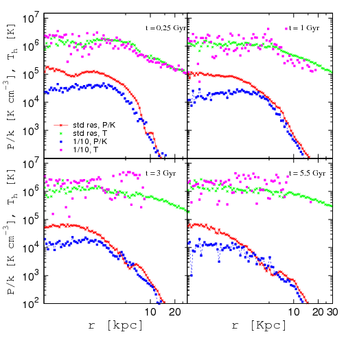
Figure 5.44: MW pressure and hot temperature profiles at standard resolution (std res) and at low resolution (1/10).

This is due to the fact that particle sampling of the gas distribution in the LR run is poor; in presence of an exponentially declining profile, less gas particles match our density threshold for entering the multi-phase regime. Quantities related to multi-phase regime, as the hot gas density and pressure (which is weighted on the total gas mass, but generated mainly by our hot gas phase, therefore show a decrease. The cold gas density and the hot temperature (which is mass-weighted over the hot mass) are instead stable. Therefore, MUPPI is still producing ISM properties which are stable against the numerical resolution. Care must however be taken, obviously, to resolution effect that doesn’t came out of the model but directly out of the SPH treatment of the hydrodynamics. We however verified that, after $5.5$ Gyr of evolution, the total gas surface density profile in our LR and standard similar and the surface density profile of the formed stellar component are remarkably similar.

Overall, the model we present proves to be very stable against variation in mass and force resolution.

5.6 Conclusions

In this section we presented and discussed the results obtained by evolving MUPPI (described in Chapter 4), our new sub-grid model of the ISM, using our reference set of parameters, in various physical conditions, i.e. a model of the Milky-Way, a model of a typical dwarf galaxy and two isolated halos, one chacteristic of the Milky-Way and one of a dwarf-like galaxy.

The main feature of our model is that it solves, for each multi-phase gas particle, a system of differential equations aimed to modelling the main physics of the ISM. It does not use equilibrium solutions for calculating ISM properties, i.e. they depend on the interplay between hot and cold gas phases, star formation and SNe energy feedback, and local thermodynamical properties, as given by the SPH code. This means that, besides following the non-equilibrium phase at the onset of the multi-phase regime, MUPPI is able to respond to changes in the local thermodynamics such as pressure/temperature changes due to compressions/rarefactions and shocks, as we showed along this Chapter.

The simulation of the Milky-Way galaxy shows good agreement with the observed Schmidt-Kennicut law (1998) and is thus able to lead to a self-regulated cycle of star formation, where mass flows in the cold phase and star formation are efficiently counterbalanced by the SNe feedback effects. We showed the evolution of single gas particles lying in different positions in the galaxy and verified how MUPPI efficiently follows the diverse evolution of their physical properties. The characteristics of the ISM we found for a particle lying at about solar distance are in reasonable agreement with observations. The gas disk develops long lasting, sharp spiral arms and part of the gas is expelled from the disk in the vertical direction, generating galactic fountains without using any ad-hoc kinetic feedback prescriptions. These results arise as a natural consequence of the ISM physics implemented in MUPPI.

Simulation of the dwarf galaxy reproduce the main physical properties expected from a quiet and lighter galaxy, with a less active ISM. Compared to the Milky-Way in fact, the star formation rate is lower, being the dwarf galaxy less massive and dense and thus less pressurised. In this case, we showed that we don’t have enough pressure to drive a “thermal wind” outside the galaxy plane.

We moreover verified that MUPPI works well in the very different physical conditions found at the centre of cooling flows. In both Milky-Way and dwarf like halos, MUPPI is able to counter the cooling flow by efficiently distributing the fraction of SNe energy in the blow out regime to neighbours: the higher the fraction of blowing out energy, the more the star formation is suppressed.

In order to assess how MUPPI respond to the choice of its parameters, we ran a set of simulations varying them in the galaxy models. Finally we tested our code against numerical resolution by simulating the Milky-way galaxy with ten times less gas and dark matter particles, as well as the dwarf-like halo with ten times more and ten times less gas and dark matter particles. We found our results are numerically stable since the general properties of the ISM does not significantly change when we vary resolution.

The model we presented here will be particularly useful in cosmological simulations of formation and evolution of isolated galaxies and galaxy clusters. In fact, it is able to capture the main ISM properties and produce an effective SNe thermal feedback, without resorting on the extreme numerical resolution needed to directly simulate the ISM.

The first application of the present Ph.D. work will therefore be to apply MUPPI to cosmological simulations, with the aim of determine how an improved treatment of star formation and feedback astrophysical processes impacts on many open issues, from the properties of simulated disk galaxies to the properties of cold baryons (galaxies and diffuse stellar component) in galaxy clusters, to the properties of the Intra-Cluster Medium in presence of an effective SNe thermal feedback.

Conclusions

If we aim in comparing galaxy formation simulations with observations, the collisionless dynamics of the dark matter particles must be coupled to gas dynamics and small-scale astrophysical processes. White & Rees in 1978 reported “An important issue in theories of galaxy formation is the relative importance of purely gravitational processes (as N-Body effects, clustering, etc..) and of gas-dynamical effects involving dissipation and radiative cooling“: the significant point they revealed 30 years ago in hierachical simulations is still an issue.

In Chapter II, we presented a comparison of various star formation and SNe feedback prescriptions in two NFW isolated, non-rotating Dark Matter halos having mass typical of a galaxy and of a poor cluster of galaxies, using the TREE+SPH code GADGET-2. The aim of this work thus was to study the behaviour of different star formation and feedback models, previously tested on disk galaxies, in very different physical conditions such those found at the centre of cooling flows.
We tested the GADGET effective star formation model (EFF), which is based on a multi-phase description of the gas contained in a particle, an implementation of the simple scheme proposed by Katz et al. 1996 (SSF), where feedback energy is given to star-forming particles in the form of thermal energy, and an implementation of Thacker & Couchman 2000 with the improvements of Stinson et al. 2006 (DEL), which consists in turning off radiative cooling for a fixed period of time of 30 Myr when the SN energy is deposited, thus mimiking the effect of SNe super-bubbles on the ISM.
Our main conclusion is that, while SN feedback in the EFF and SSF models are not efficient in countering the cooling flow and gas radiative losses at the halo centre, the DEL scheme proves quite effective at doing so. The cost of it is an unrealistic delay in the star formation history. While star formation and feedback schemes which turn off radiative cooling have proved effective in producing realistic disk galaxies in cosmological simulations, caution should therefore being used when utilising similar schemes as general-purpose ones, e.g. in galaxy cluster simulations.

In Chapter III, we have studied the origin of the diffuse stellar component in galaxy clusters taken from a cosmological hydrodynamical simulation. We found that the formation of the diffuse stellar component has no preferred redshift and is a cumulative power–law process up to redshift $z=0$. Moreover we found no correlation between the final amount of stars in the diffuse component and the global dynamical hystory of the clusters. For all but the three most massive clusters, the formation of the diffuse component has been found to go largely in parallel with the build-up of the brighest cluster galaxy. The most important result we found in this analysis is that most of the diffuse star particles become unbound during merging phases (and not by tidal stripping) along the formation history of the brighest cluster galaxy, independent of cluster mass. Such work has been performed using the standard Springel & Hernquist (2003) prescription for star formation and SNe energy feedback. An open point remains, if a more realistic treatment of the ISM physics (and thus of star formation and SNe energy feedback), leading for instance to the build-up of disk galaxies inside simulated clusters at resolutions that simulation of this kind can routinely reach, would change our conclusions.

This is only an example of how important in many astrophysical problems a proper treatment of the ISM physics in cosmological simulations may be. The main aim of this Ph.D. Thesis work has been introducing a sofisticated model for following the complex astrophysical processes acting in the interstellar medium in numerical simulations involving galaxy formations.

We fullly describe our model, called MUPPI, $\boldsymbol{MU}$lti$\boldsymbol{P}$hase $\boldsymbol{P}$article $\boldsymbol{I}$ntegrator, in Chapter IV. MUPPI follows the ISM physics using a system of ordinary differential equations, describing mass and energy flows among the different gas phases in the ISM inside each gas particle. The model also includes the treatment of SNe energy transfer from star-forming particles to their neighbours.

Along Chapter V, we presented and discussed the results obtained evolving various physical cases with MUPPI. We simulated an isolated model of the Milky-Way, a model of a typical dwarf galaxy and two isolated cooling-flows halos without galaxies, one having the same chacteristic of the Milky-Way halo and another of a dwarf-like galaxy. The overall result we found in these simulations is that MUPPI is successfull in properly following the inter stellar medium evolution in very different physical situations. In particular, the simulation of the Milky-Way galaxy shows good agreement with the observed Schmidt-Kennicut law (1998) and is thus able to lead to a self-regulated cycle of star formation, where mass flows in the cold phase and star formation are efficiently counterbalanced by the supernova feedback effects. The characteristics of the interstellar medium we found for a particle lying at about solar distance are in reasonable agreement with observations. Moreover, heated gas is expelled from the disk in the vertical direction and then falls back, generates galactic fountains. These results arise as a natural consequence of the interstellar medium physics as implemented in MUPPI. Thermal feedback is thus very effective in our implementation, a result that other sub-grid star formation recipes don’t get, or obtain only with ad-hoc parametrization (as e.g. in Stinson et al 2006 work) or resorting to ad-hoc kinetic feedback (e.g. Springel & Hernquist 2003).

In order to test the MUPPI code behaviour on different initial physical conditions, we runned a simulation of the dwarf galaxy and we found that results reproduce the main physical properties expected from a quiet and less massive galaxy, with a less active intestellar medium.
Moreover MUPPI works well even in the very different physical conditions found at the centre of isolated halos, where our code has been found to be able to efficiently counter the cooling flow.
In order to assess how MUPPI respond to the choice of its parameters, we ran a set of simulations varying them in the galaxy models. Finally we tested our code against numerical resolution by simulating the Milky-way galaxy with a ten times worse mass resolution, as well as the dwarf-like halo with ten times more and ten times less gas and dark matter particles. We found our results are numerically stable: the general properties of the simulated interstellar medium does not significantly change when we vary resolution. This is a particularly important point, as our model is intended for use in simulations where an extreme mass and force resolution can’t be reached given the present-day available computing power.

We believe the model we presented here will be particularly useful in cosmological simulations of formation and evolution of isolated galaxies and galaxy clusters. For this reason, the first application of the present Ph.D. work will therefore be to apply MUPPI to cosmological simulations, with the aim of determine how an improved treatment of star formation and feedback astrophysical processes impacts on many open issues, from the properties of simulated disk galaxies to the properties of cold baryons (galaxies and diffuse stellar component) in galaxy clusters, to the properties of the Intra-Cluster Medium in presence of an effective supernovae thermal feedback.

References

- [1] Abadi, M. G., Navarro, J. F., and Steinmetz, M. Stars beyond galaxies: the origin of extended luminous haloes around galaxies. MNRAS365 (Jan. 2006), 747–758.
- [2] Abell, G. O. The Distribution of Rich Clusters of Galaxies. ApJS3 (May 1958), 211–+.
- [3] Abell, G. O. Clustering of Galaxies. ARA&A3 (1965), 1–+.
- [4] Abell, G. O., Corwin, H. G., and Olowin, R. P. A catalog of rich clusters of galaxies. ApJS70 (May 1989), 1–138.
- [5] Aguerri, J. A. L., Castro-Rodríguez, N., Napolitano, N., Arnaboldi, M., and Gerhard, O. Diffuse light in Hickson compact groups: the dynamically young system HCG 44. A&A457 (Oct. 2006), 771–778.
- [6] Aguerri, J. A. L., Gerhard, O. E., Arnaboldi, M., Napolitano, N. R., Castro-Rodriguez, N., and Freeman, K. C. Intracluster Stars in the Virgo Cluster Core. AJ129 (June 2005), 2585–2596.
- [7] Allen, S. W., Schmidt, R. W., and Fabian, A. C. The X-ray virial relations for relaxed lensing clusters observed with Chandra. MNRAS328 (Dec. 2001), L37–L41.
- [8] Arnaboldi, M., Aguerri, J. A. L., Napolitano, N. R., Gerhard, O., Freeman, K. C., Feldmeier, J., Capaccioli, M., Kudritzki, R. P., and Méndez, R. H. Intracluster Planetary Nebulae in Virgo: Photometric Selection, Spectroscopic Validation, and Cluster Depth. AJ123 (Feb. 2002), 760–771.
- [9] Arnaboldi, M., Freeman, K. C., Okamura, S., Yasuda, N., Gerhard, O., Napolitano, N. R., and Pannella, M. E. Narrowband Imaging in [O III] and H to Search for Intracluster Planetary Nebulae in the Virgo Cluster. AJ125 (Feb. 2003), 514–524.
- [10] Arnaboldi, M., Gerhard, O., Aguerri, J. A. L., Freeman, K. C., Napolitano, N. R., Okamura, S., and Yasuda, N. The Line-of-Sight Velocity Distributions of Intracluster Planetary Nebulae in the Virgo Cluster Core. ApJ614 (Oct. 2004), L33–L36.
- [11] Balogh, M. L., Babul, A., and Patton, D. R. Pre-heated isentropic gas in groups of galaxies. MNRAS307 (Aug. 1999), 463–479.
- [12] Balogh, M. L., Pearce, F. R., Bower, R. G., and Kay, S. T. Revisiting the cosmic cooling crisis. MNRAS326 (Oct. 2001), 1228–1234.
- [13] Baron, E., and White, S. D. M. The appearance of primeval galaxies. ApJ322 (Nov. 1987), 585–596.
- [14] Begelman, M. C. AGN feedback mechanism. ArXiv Astrophysics e-prints (Mar. 2003).
- [15] Bernstein, G. M., Nichol, R. C., Tyson, J. A., Ulmer, M. P., and Wittman, D. The Luminosity Function of the Coma Cluster Core for . AJ110 (Oct. 1995), 1507–+.
- [16] Bialek, J. J., Evrard, A. E., and Mohr, J. J. Effects of Preheating on X-Ray Scaling Relations in Galaxy Clusters. ApJ555 (July 2001), 597–612.
- [17] Böhringer, H., Collins, C. A., Guzzo, L., Schuecker, P., Voges, W., Neumann, D. M., Schindler, S., Chincarini, G., De Grandi, S., Cruddace, R. G., Edge, A. C., Reiprich, T. H., and Shaver, P. The ROSAT-ESO Flux-limited X-Ray (REFLEX) Galaxy Cluster Survey. IV. The X-Ray Luminosity Function. ApJ566 (Feb. 2002), 93–102.
- [18] Booth, C. M., Theuns, T., and Okamoto, T. Molecular cloud regulated star formation in galaxies. MNRAS376 (Apr. 2007), 1588–1610.
- [19] Borgani, S. Cosmology with clusters of galaxies. ArXiv Astrophysics e-prints (May 2006).
- [20] Borgani, S., Dolag, K., Murante, G., Cheng, L.-M., Springel, V., Diaferio, A., Moscardini, L., Tormen, G., Tornatore, L., and Tozzi, P. Hot and cooled baryons in smoothed particle hydrodynamic simulations of galaxy clusters: physics and numerics. MNRAS367 (Apr. 2006), 1641–1654.
- [21] Borgani, S., Governato, F., Wadsley, J., Menci, N., Tozzi, P., Lake, G., Quinn, T., and Stadel, J. Preheating the Intracluster Medium in High-Resolution Simulations: The Effect on the Gas Entropy. ApJ559 (Oct. 2001), L71–L74.
- [22] Borgani, S., and Guzzo, L. X-ray clusters of galaxies as tracers of structure in the Universe. Nature409 (Jan. 2001), 39–45.
- [23] Borgani, S., Murante, G., Springel, V., Diaferio, A., Dolag, K., Moscardini, L., Tormen, G., Tornatore, L., and Tozzi, P. X-ray properties of galaxy clusters and groups from a cosmological hydrodynamical simulation. MNRAS348 (Mar. 2004), 1078–1096.
- [24] Borgani, S., Rosati, P., Tozzi, P., Stanford, S. A., Eisenhardt, P. R., Lidman, C., Holden, B., Della Ceca, R., Norman, C., and Squires, G. Measuring with the ROSAT Deep Cluster Survey. ApJ561 (Nov. 2001), 13–21.
- [25] Brighenti, F., and Mathews, W. G. Entropy Evolution in Galaxy Groups and Clusters: a Comparison of External and Internal Heating. ApJ553 (May 2001), 103–120.
- [26] Byrd, G., and Valtonen, M. Tidal generation of active spirals and S0 galaxies by rich clusters. ApJ350 (Feb. 1990), 89–94.
- [27] Carlberg, R. G., Yee, H. K. C., and Ellingson, E. The Average Mass and Light Profiles of Galaxy Clusters. ApJ478 (Mar. 1997), 462–+.
- [28] Castro-Rodríguez, N., Aguerri, J. A. L., Arnaboldi, M., Gerhard, O., Freeman, K. C., Napolitano, N. R., and Capaccioli, M. Narrow band survey for intragroup light in the Leo HI cloud. Constraints on the galaxy background contamination in imaging surveys for intracluster planetary nebulae. A&A405 (July 2003), 803–812.
- [29] Cavaliere, A., and Fusco-Femiano, R. X-rays from hot plasma in clusters of galaxies. A&A49 (May 1976), 137–144.
- [30] Cavaliere, A., Menci, N., and Tozzi, P. Diffuse Baryons in Groups and Clusters of Galaxies. ApJ501 (July 1998), 493–+.
- [31] Cen, R., and Ostriker, J. A hydrodynamic treatment of the cold dark matter cosmological scenario. ApJ393 (July 1992), 22–41.
- [32] Coles, P., and Lucchin, F. Cosmology: The Origin and Evolution of Cosmic Structure, Second Edition. Cosmology: The Origin and Evolution of Cosmic Structure, Second Edition, by Peter Coles, Francesco Lucchin, pp. 512. ISBN 0-471-48909-3. Wiley-VCH , July 2002., July 2002.
- [33] Cypriano, E. S., Sodré, L. J., Campusano, L. E., Dale, D. A., and Hardy, E. Shrinking of Cluster Ellipticals: A Tidal Stripping Explanation and Implications for the Intracluster Light. AJ131 (May 2006), 2417–2425.
- [34] Dalla Vecchia, C., and Schaye, J. Simulating galactic outflows with kinetic supernova feedback. MNRAS387 (July 2008), 1431–1444.
- [35] Davis, M., and Peebles, P. J. E. A survey of galaxy redshifts. V - The two-point position and velocity correlations. ApJ267 (Apr. 1983), 465–482.
- [36] De Grandi, S., and Molendi, S. Temperature Profiles of Nearby Clusters of Galaxies. ApJ567 (Mar. 2002), 163–177.
- [37] de Vaucouleurs, G. The Apparent Density of Matter in Groups and Clusters of Galaxies. ApJ131 (May 1960), 585–+.
- [38] de Vaucouleurs, G. Photometry of the Outer Corona of Messier 87. ApJ4 (1969), 17–+.
- [39] Dolag, K., Borgani, S., Schindler, S., Diaferio, A., and Bykov, A. M. Simulation Techniques for Cosmological Simulations. Space Science Reviews 134 (Feb. 2008), 229–268.
- [40] D’Onghia, E., Sommer-Larsen, J., Romeo, A. D., Burkert, A., Pedersen, K., Portinari, L., and Rasmussen, J. The Formation of Fossil Galaxy Groups in the Hierarchical Universe. ApJ630 (Sept. 2005), L109–L112.
- [41] Eisenstein, D. J., and Hu, W. Power Spectra for Cold Dark Matter and Its Variants. ApJ511 (Jan. 1999), 5–15.
- [42] Eke, V. R., Cole, S., and Frenk, C. S. Cluster evolution as a diagnostic for Omega. MNRAS282 (Sept. 1996), 263–280.
- [43] Evrard, A. E., and Henry, J. P. Expectations for X-ray cluster observations by the ROSAT satellite. ApJ383 (Dec. 1991), 95–103.
- [44] Evrard, A. E., Metzler, C. A., and Navarro, J. F. Mass Estimates of X-Ray Clusters. ApJ469 (Oct. 1996), 494–+.
- [45] Fabian, A. C. Cooling Flows in Clusters of Galaxies. ARA&A32 (1994), 277–318.
- [46] Fabian, A. C., Mushotzky, R. F., Nulsen, P. E. J., and Peterson, J. R. On the soft X-ray spectrum of cooling flows. MNRAS321 (Feb. 2001), L20–L24.
- [47] Feldmeier, J. J., Ciardullo, R., Jacoby, G. H., and Durrell, P. R. Intracluster Planetary Nebulae in the Virgo Cluster. II. Imaging Catalog. ApJS145 (Mar. 2003), 65–81.
- [48] Feldmeier, J. J., Ciardullo, R., Jacoby, G. H., and Durrell, P. R. Intracluster Planetary Nebulae in the Virgo Cluster. III. Luminosity of the Intracluster Light and Tests of the Spatial Distribution. ApJ615 (Nov. 2004), 196–208.
- [49] Feldmeier, J. J., Mihos, J. C., Durrell, P. R., Ciardullo, R., and Jacoby, G. H. Kinematics of Planetary Nebulae in M51’s Tidal Tail. In IAU Symposium (2003), S. Kwok, M. Dopita, and R. Sutherland, Eds., pp. 633–+.
- [50] Feldmeier, J. J., Mihos, J. C., Morrison, H. L., Rodney, S. A., and Harding, P. Deep CCD Surface Photometry of Galaxy Clusters. I. Methods and Initial Studies of Intracluster Starlight. ApJ575 (Aug. 2002), 779–800.
- [51] Gal-Yam, A., Maoz, D., Guhathakurta, P., and Filippenko, A. V. A Population of Intergalactic Supernovae in Galaxy Clusters. AJ125 (Mar. 2003), 1087–1094.
- [52] Gallagher, III, J. S., and Ostriker, J. P. A Note on Mass Loss during Collisions between Galaxies a nd the Formation of Giant Systems. AJ77 (May 1972), 288–+.
- [53] Gebhardt, K., and Beers, T. C. Bound populations around cD galaxies and cD velocity offsets in clusters of galaxies. ApJ383 (Dec. 1991), 72–89.
- [54] Gerhard, O., Arnaboldi, M., Freeman, K. C., Kashikawa, N., Okamura, S., and Yasuda, N. Detection of Intracluster Planetary Nebulae in the Coma Cluster. ApJ621 (Mar. 2005), L93–L96.
- [55] Gerritsen, J. P. E., and Icke, V. Star formation in N-body simulations. I. The impact of the stellar ultraviolet radiation on star formation. A&A325 (Sept. 1997), 972–986.
- [56] Gioia, I. M., Henry, J. P., Mullis, C. R., Ebeling, H., and Wolter, A. RX J1716.6+6708: A Young Cluster at Z=0.81. AJ117 (June 1999), 2608–2616.
- [57] Girardi, M., and Mezzetti, M. Evolution of the Internal Dynamics of Galaxy Clusters. ApJ548 (Feb. 2001), 79–96.
- [58] Gnedin, O. Y. Dynamical Evolution of Galaxies in Clusters. ApJ589 (June 2003), 752–769.
- [59] Gonzalez, A. H., Zabludoff, A. I., Zaritsky, D., and Dalcanton, J. J. Measuring the Diffuse Optical Light in Abell 1651. ApJ536 (June 2000), 561–570.
- [60] Governato, F., Willman, B., Mayer, L., Brooks, A., Stinson, G., Valenzuela, O., Wadsley, J., and Quinn, T. Forming disc galaxies in CDM simulations. MNRAS374 (Feb. 2007), 1479–1494.
- [61] Gunn, J. E. Visual Background Radiation in the Coma Cluster of Galaxies. In Bulletin of the American Astronomical Society (Mar. 1969), vol. 1 of Bulletin of the American Astronomical Society, pp. 191–+.
- [62] Haardt, F., and Madau, P. Radiative Transfer in a Clumpy Universe. II. The Ultraviolet Extragalactic Background. ApJ461 (Apr. 1996), 20–+.
- [63] Hernquist, L. An analytical model for spherical galaxies and bulges. ApJ356 (June 1990), 359–364.
- [64] Hernquist, L. N-body realizations of compound galaxies. ApJS86 (June 1993), 389–400.
- [65] Holmberg, E. A photographic photometry of extragalactic nebulae. Meddelanden fran Lunds Astronomiska Observatorium Serie II 136 (1958), 1–+.
- [66] Irwin, J. A., and Bregman, J. N. Radial Temperature Profiles of 11 Clusters of Galaxies Observed with BEPPOSAX. ApJ538 (Aug. 2000), 543–554.
- [67] Jeltema, T. E., Canizares, C. R., Bautz, M. W., Malm, M. R., Donahue, M., and Garmire, G. P. Chandra X-Ray Observatory Observation of the High-Redshift Cluster MS 1054-0321. ApJ562 (Nov. 2001), 124–132.
- [68] Kaiser, N. Evolution and clustering of rich clusters. MNRAS222 (Sept. 1986), 323–345.
- [69] Katz, N. Dissipational galaxy formation. II - Effects of star formation. ApJ391 (June 1992), 502–517.
- [70] Katz, N., Weinberg, D. H., and Hernquist, L. Cosmological Simulations with TreeSPH. ApJS105 (July 1996), 19.
- [71] Kauffmann, G. Formation Histories Expected From Cosmological Simulations. In ASP Conf. Ser. 245: Astrophysical Ages and Times Scales (2001), T. von Hippel, C. Simpson, and N. Manset, Eds., pp. 381–+.
- [72] Kay, S. T., da Silva, A. C., Aghanim, N., Blanchard, A., Liddle, A. R., Puget, J.-L., Sadat, R., and Thomas, P. A. The evolution of clusters in the CLEF cosmological simulation: X-ray structural and scaling properties. MNRAS377 (May 2007), 317–334.
- [73] Kennicutt, Jr., R. C. The Global Schmidt Law in Star-forming Galaxies. ApJ498 (May 1998), 541–+.
- [74] Komatsu, E., and Seljak, U. Universal gas density and temperature profile. MNRAS327 (Nov. 2001), 1353–1366.
- [75] Krick, J. E., Bernstein, R. A., and Pimbblet, K. A. Diffuse Optical Light in Galaxy Clusters. I. Abell 3888. AJ131 (Jan. 2006), 168–184.
- [76] Lewis, A. D., Ellingson, E., Morris, S. L., and Carlberg, R. G. X-Ray Mass Estimates at Z ~ 0.3 for the Canadian Network for Observational Cosmology Cluster Sample. ApJ517 (June 1999), 587–608.
- [77] Lin, Y.-T., Mohr, J. J., and Stanford, S. A. Near-Infrared Properties of Galaxy Clusters: Luminosity as a Binding Mass Predictor and the State of Cluster Baryons. ApJ591 (July 2003), 749–763.
- [78] Lin, Y.-T., Mohr, J. J., and Stanford, S. A. K-Band Properties of Galaxy Clusters and Groups: Luminosity Function, Radial Distribution, and Halo Occupation Number. ApJ610 (Aug. 2004), 745–761.
- [79] Lloyd-Davies, E. J., Ponman, T. J., and Cannon, D. B. The entropy and energy of intergalactic gas in galaxy clusters. MNRAS315 (July 2000), 689–702.
- [80] Mackie, G. The stellar content of central dominant galaxies. II - Colors of cD envelopes. ApJ400 (Nov. 1992), 65–73.
- [81] Markevitch, M., Forman, W. R., Sarazin, C. L., and Vikhlinin, A. The Temperature Structure of 30 Nearby Clusters Observed with ASCA: Similarity of Temperature Profiles. ApJ503 (Aug. 1998), 77–+.
- [82] Marri, S., and White, S. D. M. Smoothed particle hydrodynamics for galaxy-formation simulations: improved treatments of multiphase gas, of star formation and of supernovae feedback. MNRAS345 (Oct. 2003), 561–574.
- [83] Matzner, C. D. On the Role of Massive Stars in the Support and Destruction of Giant Molecular Clouds. ApJ566 (Feb. 2002), 302–314.
- [84] Merritt, D. Relaxation and tidal stripping in rich clusters of galaxies. II - Evolution of the luminosity distribution. ApJ276 (Jan. 1984), 26–37.
- [85] Merritt, D. Dynamical Modelling of Hot Stellar Systems. ArXiv Astrophysics e-prints (Oct. 1995).
- [86] Mihos, J. C. Interactions and Mergers of Cluster Galaxies. In Clusters of Galaxies: Probes of Cosmological Structure and Galaxy Evolution (2004), J. S. Mulchaey, A. Dressler, and A. Oemler, Eds., pp. 277–+.
- [87] Mihos, J. C., Harding, P., Feldmeier, J., and Morrison, H. Diffuse Light in the Virgo Cluster. ApJ631 (Sept. 2005), L41–L44.
- [88] Monaco, P. Physical regimes for feedback in galaxy formation. MNRAS352 (July 2004), 181–204.
- [89] Monaco, P., Fontanot, F., and Taffoni, G. The MORGANA model for the rise of galaxies and active nuclei. ArXiv Astrophysics e-prints (Oct. 2006).
- [90] Monaco, P., Murante, G., Borgani, S., and Fontanot. Diffuse Stellar Component in Galaxy Clusters and the Evolution of the Most Massive Galaxies at z ¡ ~1. ApJ652 (Dec. 2006), L89–L92.
- [91] Moore, B., Katz, N., Lake, G., Dressler, A., and Oemler, A. Galaxy harassment and the evolution of clusters of galaxies. Nature379 (1996), 613–616.
- [92] Murante, G., Arnaboldi, M., Gerhard, O., Borgani, S., Cheng, L. M., Diaferio, A., Dolag, K., Moscardini, L., Tormen, G., Tornatore, L., and Tozzi, P. The Diffuse Light in Simulations of Galaxy Clusters. ApJ607 (June 2004), L83–L86.
- [93] Nagai, D., Kravtsov, A. V., and Vikhlinin, A. Effects of Galaxy Formation on Thermodynamics of the Intracluster Medium. ApJ668 (Oct. 2007), 1–14.
- [94] Napolitano, N. R., Pannella, M., Arnaboldi, M., Gerhard, O., Aguerri, J. A. L., Freeman, K. C., Capaccioli, M., Ghigna, S., Governato, F., Quinn, T., and Stadel, J. Intracluster Stellar Population Properties from N-Body Cosmological Simulations. I. Constraints at z = 0. ApJ594 (Sept. 2003), 172–185.
- [95] Navarro, J., Frenk, C., and White, S. The structure of cold dark matter halos. ApJ 462 (1996), 563.
- [96] Navarro, J., Frenk, C., and White, S. A universal density profile from hierarchical clustering. ApJ 490 (1997), 493.
- [97] Navarro, J. F., Frenk, C. S., and White, S. D. M. Simulations of X-ray clusters. MNRAS275 (Aug. 1995), 720–740.
- [98] Navarro, J. F., and White, S. D. M. Simulations of Dissipative Galaxy Formation in Hierarchically Clustering Universes - Part One - Tests of the Code. MNRAS265 (Nov. 1993), 271–+.
- [99] Ostriker, J. P., and Hausman, M. A. Cannibalism among the galaxies - Dynamically produced evolution of cluster luminosity functions. ApJ217 (Nov. 1977), L125–L129.
- [100] Ostriker, J. P., and Steinhardt, P. New Light on Dark Matter. Science 300 (June 2003), 1909–1914.
- [101] Peacock, J. A. Cosmological Physics. Cosmological Physics, by John A. Peacock, pp. 704. ISBN 052141072X. Cambridge, UK: Cambridge University Press, January 1999., Jan. 1999.
- [102] Peebles, P. J. E. Principles of physical cosmology. Princeton Series in Physics, Princeton, NJ: Princeton University Press, —c1993, 1993.
- [103] Perlmutter, S., Turner, M. S., and White, M. Constraining Dark Energy with Type Ia Supernovae and Large-Scale Structure. Physical Review Letters 83 (July 1999), 670–673.
- [104] Peterson, J. R., Paerels, F. B. S., Kaastra, J. S., Arnaud, M., Reiprich, T. H., Fabian, A. C., Mushotzky, R. F., Jernigan, J. G., and Sakelliou, I. X-ray imaging-spectroscopy of Abell 1835. A&A365 (Jan. 2001), L104–L109.
- [105] Ponman, T. J., Cannon, D. B., and Navarro, J. F. The thermal imprint of galaxy formation on X-ray clusters. Nature397 (Jan. 1999), 135–137.
- [106] Power, C., Navarro, J., Jenkins, A., Frenk, C., White, S., Springel, V., Stadel, J., and Quinn, T. The inner structure of cdm haloes - i. a numerical convergence study. MNRAS 338 (2003), 14.
- [107] Press, W. H., and Schechter, P. Formation of Galaxies and Clusters of Galaxies by Self-Similar Gravitational Condensation. ApJ187 (Feb. 1974), 425–438.
- [108] Press, W. H., Teukolsky, S. A., Vetterling, W. T., and Flannery, B. P. Numerical recipes in C. The art of scientific computing. Cambridge: University Press, —c1992, 2nd ed., 1992.
- [109] Prestwich, A. H., and Joy, M. Cooling flows and the formation of massive halos in cD galaxies. ApJ369 (Mar. 1991), L1–L4.
- [110] Raymond, J. C., and Smith, B. W. Soft X-ray spectrum of a hot plasma. ApJS35 (Dec. 1977), 419–439.
- [111] Reiprich, T. H., and Böhringer, H. The Mass Function of an X-Ray Flux-limited Sample of Galaxy Clusters. ApJ567 (Mar. 2002), 716–740.
- [112] Rosati, P., Borgani, S., and Norman, C. The Evolution of X-ray Clusters of Galaxies. ARA&A40 (2002), 539–577.
- [113] Rudick, C. S., Mihos, J. C., and McBride, C. The Formation and Evolution of Intracluster Light. ApJ648 (Sept. 2006), 936–946.
- [114] Sakharov, A. S., and Hofer, H. Development of the Universe and New Cosmology. ArXiv Astrophysics e-prints (Sept. 2003).
- [115] Sarazin, C. L. X-ray emission from clusters of galaxies. Cambridge University Press, Cambridge, 1988.
- [116] Scannapieco, C., Tissera, P. B., White, S. D. M., and Springel, V. Feedback and metal enrichment in cosmological smoothed particle hydrodynamics simulations - I. A model for chemical enrichment. MNRAS364 (Dec. 2005), 552–564.
- [117] Scannapieco, C., Tissera, P. B., White, S. D. M., and Springel, V. Feedback and metal enrichment in cosmological SPH simulations - II. A multiphase model with supernova energy feedback. MNRAS371 (Sept. 2006), 1125–1139.
- [118] Scheick, X., and Kuhn, J. R. Diffuse Light in A2670: Smoothly Distributed? ApJ423 (Mar. 1994), 566–+.
- [119] Schombert, J. M. The structure of brightest cluster members. III - cD envelopes. ApJ328 (May 1988), 475–488.
- [120] Sedov, L. I. Similarity and Dimensional Methods in Mechanics. Similarity and Dimensional Methods in Mechanics, New York: Academic Press, 1959, 1959.
- [121] Shen, S., Mo, H. J., White, S. D. M., Blanton, M. R., Kauffmann, G., Voges, W., Brinkmann, J., and Csabai, I. The size distribution of galaxies in the Sloan Digital Sky Survey. MNRAS343 (Aug. 2003), 978–994.
- [122] Sheth, R. K., Mo, H. J., and Tormen, G. Ellipsoidal collapse and an improved model for the number and spatial distribution of dark matter haloes. MNRAS323 (May 2001), 1–12.
- [123] Smith, S. The Mass of the Virgo Cluster. ApJ83 (Jan. 1936), 23–+.
- [124] Smoluchowski, M. V. Drei Vortrage uber Diffusion, Brownsche Bewegung und Koagulation von Kolloidteilchen. Zeitschrift fur Physik 17 (1916), 557–585.
- [125] Sommer-Larsen, J. Properties of intra-group stars and galaxies in galaxy groups: ‘normal’ versus ‘fossil’ groups. MNRAS (June 2006), 509–+.
- [126] Sommer-Larsen, J., Romeo, A. D., and Portinari, L. Simulating galaxy clusters - III. Properties of the intracluster stars. MNRAS357 (Feb. 2005), 478–488.
- [127] Springel, V. The cosmological simulation code GADGET-2. MNRAS364 (Dec. 2005), 1105–1134.
- [128] Springel, V., Di Matteo, T., and Hernquist, L. Modelling feedback from stars and black holes in galaxy mergers. MNRAS361 (Aug. 2005), 776–794.
- [129] Springel, V., and Hernquist, L. Cosmological smoothed particle hydrodynamics simulations: the entropy equation. MNRAS333 (July 2002), 649–664.
- [130] Springel, V., and Hernquist, L. Cosmological smoothed particle hydrodynamics simulations: a hybrid multiphase model for star formation. MNRAS339 (Feb. 2003), 289–311.
- [131] Springel, V., White, S. D. M., Tormen, G., and Kauffmann, G. Populating a cluster of galaxies - I. Results at z=0. MNRAS328 (Dec. 2001), 726–750.
- [132] Springel, V., Yoshida, N., and White, S. D. M. GADGET: a code for collisionless and gasdynamical cosmological simulations. New Astronomy 6 (Apr. 2001), 79–117.
- [133] Stadel, J. G. Cosmological N-body simulations and their analysis. Ph.D. Thesis (2001).
- [134] Stinson, G., Seth, A., Katz, N., Wadsley, J., Governato, F., and Quinn, T. Star formation and feedback in smoothed particle hydrodynamic simulations - I. Isolated galaxies. MNRAS373 (Dec. 2006), 1074–1090.
- [135] Sutherland, R. S., and Dopita, M. A. Cooling functions for low-density astrophysical plasmas. ApJS88 (Sept. 1993), 253–327.
- [136] Suto, Y., Sasaki, S., and Makino, N. Gas Density and X-Ray Surface Brightness Profiles of Clusters of Galaxies from Dark Matter Halo Potentials: Beyond the Isothermal beta-Model. ApJ509 (Dec. 1998), 544–550.
- [137] Tamura, T., Kaastra, J. S., Peterson, J. R., Paerels, F. B. S., Mittaz, J. P. D., Trudolyubov, S. P., Stewart, G., Fabian, A. C., Mushotzky, R. F., Lumb, D. H., and Ikebe, Y. X-ray spectroscopy of the cluster of galaxies Abell 1795 with XMM-Newton. A&A365 (Jan. 2001), L87–L92.
- [138] Thacker, R. J., and Couchman, H. M. P. Implementing Feedback in Simulations of Galaxy Formation: A Survey of Methods. ApJ545 (Dec. 2000), 728–752.
- [139] Thuan, T. X., and Romanishin, W. The structure of giant elliptical galaxies in poor clusters of galaxies. ApJ248 (Sept. 1981), 439–459.
- [140] Tonry, J. L., Schmidt, B. P., Barris, B., Candia, P., Challis, P., Clocchiatti, A., Coil, A. L., Filippenko, A. V., Garnavich, P., Hogan, C., Holland, S. T., Jha, S., Kirshner, R. P., Krisciunas, K., Leibundgut, B., Li, W., Matheson, T., Phillips, M. M., Riess, A. G., Schommer, R., Smith, R. C., Sollerman, J., Spyromilio, J., Stubbs, C. W., and Suntzeff, N. B. Cosmological Results from High-z Supernovae. ApJ594 (Sept. 2003), 1–24.
- [141] Tormen, G., Bouchet, F. R., and White, S. D. M. The structure and dynamical evolution of dark matter haloes. MNRAS286 (Apr. 1997), 865–884.
- [142] Tozzi, P., and Norman, C. The Evolution of X-Ray Clusters and the Entropy of the Intracluster Medium. ApJ546 (Jan. 2001), 63–84.
- [143] Tozzi, P., Scharf, C., and Norman, C. Detection of the Entropy of the Intergalactic Medium: Accretion Shocks in Clusters, Adiabatic Cores in Groups. ApJ542 (Oct. 2000), 106–119.
- [144] Uson, J. M., Boughn, S. P., and Kuhn, J. R. Diffuse light in dense clusters of galaxies. I - R-band observations of Abell 2029. ApJ369 (Mar. 1991), 46–53.
- [145] Valentijn, E. A. Calibrated B, V surface photometry of X-ray cD galaxies. A&A118 (Feb. 1983), 123–138.
- [146] Vilchez-Gomez, R., Pello, R., and Sanahuja, B. Detection of intracluster light in the rich clusters of galaxies Abell 2390 and CL 1613+31. A&A283 (Mar. 1994), 37–50.
- [147] Villumsen, J. V. Simulations of galaxy mergers. MNRAS199 (May 1982), 493–516.
- [148] Villumsen, J. V. Simulations of galaxy mergers. II. MNRAS204 (July 1983), 219–236.
- [149] Viola, M., Monaco, P., Borgani, S., Murante, G., and Tornatore, L. How does gas cool in dark matter haloes? MNRAS383 (Jan. 2008), 777–790.
- [150] Wechsler, R. H., Bullock, J. S., Primack, J. R., Kravtsov, A. V., and Dekel, A. Concentrations of Dark Halos from Their Assembly Histories. ApJ568 (Mar. 2002), 52–70.
- [151] White, D. A. Deconvolution of ASCA X-ray data - II. Radial temperature and metallicity profiles for 106 galaxy clusters. MNRAS312 (Mar. 2000), 663–688.
- [152] Willman, B., Governato, F., Wadsley, J., and Quinn, T. The origin and properties of intracluster stars in a rich cluster. MNRAS355 (Nov. 2004), 159–168.
- [153] Wilson, C. D., and Scoville, N. The properties of individual giant molecular clouds in M33. ApJ363 (Nov. 1990), 435–450.
- [154] Wu, K. K. S., Fabian, A. C., and Nulsen, P. E. J. Non-gravitational heating in the hierarchical formation of X-ray clusters. MNRAS318 (Nov. 2000), 889–912.
- [155] Wu, X.-P., Xue, Y.-J., and Fang, L.-Z. The L_X-T and L_X- Relationships for Galaxy Clusters Revisited. ApJ524 (Oct. 1999), 22–30.
- [156] Yepes, G., Kates, R., Khokhlov, A., and Klypin, A. Hydrodynamical simulations of galaxy formation: effects of supernova feedback. MNRAS284 (Jan. 1997), 235–256.
- [157] Zibetti, S., White, S. D. M., Schneider, D. P., and Brinkmann, J. Intergalactic stars in z~ 0.25 galaxy clusters: systematic properties from stacking of Sloan Digital Sky Survey imaging data. MNRAS358 (Apr. 2005), 949–967.
- [158] Zwicky, F. On the Masses of Nebulae and of Clusters of Nebulae. ApJ86 (Oct. 1937), 217–+.
- [159] Zwicky, F. The Coma Cluster of Galaxies. PASP 63 (Apr. 1951), 61–+.
- [160] Zwicky, F. Morphological astronomy. Berlin: Springer, 1957, 1957.
- [161] Zwicky, F. Clusters of Galaxies. Handbuch der Physik 53 (1959), 390–+.
- [162] Zwicky, F., Herzog, E., and Wild, P. Catalogue of galaxies and of clusters of galaxies, Vol. 3. Pasadena: California Institute of Technology (CIT), —c1966, 1966.