GALEX–SDSS Catalogs for Statistical Studies

Abstract

We present a detailed study of the Galaxy Evolution Explorer’s photometric catalogs with special focus on the statistical properties of the All-sky and Medium Imaging Surveys. We introduce the concept of primaries to resolve the issue of multiple detections and follow a geometric approach to define clean catalogs with well-understood selection functions. We cross-identify the GALEX sources (GR2+3) with Sloan Digital Sky Survey (DR6) observations, which indirectly provides an invaluable insight about the astrometric model of the UV sources and allows us to revise the band merging strategy. We derive the formal description of the GALEX footprints as well as their intersections with the SDSS coverage along with analytic calculations of their areal coverage. The crossmatch catalogs are made available for the public. We conclude by illustrating the implementation of typical selection criteria in SQL for catalog subsets geared toward statistical analyses, e.g., correlation and luminosity function studies.

1. Introduction

The ultraviolet (UV) range of the spectrum is a tracer of recent star formation within galaxies (e.g., Kennicutt, 1998). It has been intensively used (e.g., Giavalisco, 2002) at high redshifts to study the properties of galaxies selected from the Lyman Break technique (Steidel et al., 1995). As the restframe UV light at $z\lesssim 1$ is not observable from Earth, the UV properties of objects have been better known in the distant Universe than in the local Universe. Since the launch of the Galaxy Evolution Explorer (GALEX; Martin et al., 2005), a NASA small explorer satellite designed and built to image the sky in the ultraviolet at $z<1$, a new window has been opened to connect low and high redshift UV observations. UV data are of primary interest for studying star formation over timescales of about 100 Myrs, and low redshift UV data are useful to interpret similar high redshift data. The GALEX measurements themselves, however, do not provide enough information for most studies due to the lack of angular resolution and narrow spectral coverage, which do not allow for a reliable star–galaxy separation. The single color of the two bands is also a serious restriction on the potential applications. The solution is to cross-identify the GALEX sources to other catalogs, in particular to the Sloan Digital Sky Survey (SDSS; York et al., 2000). Most GALEX observations are designed to cover regions of the sky already observed by the SDSS at a comparable depth.

In Seibert et al. (2005) and Bianchi et al. (2005, 2007) we have discussed various aspects of the associated catalogs for preliminary data releases. Existing GALEX catalogs have a number of shortcomings that include the non-uniqueness of sources detected and multiple fields. Building on the experience from a series of previous studies, we systematically analyze the issues of GALEX catalog creation in conjunction with the SDSS datasets to define a clean sample optimized for statistical studies. The impact of this new compilation is most significant on applications that require a good understanding of the selection effects and rely on the knowledge of the precise coverage of the survey, e.g., clustering and luminosity function studies.

The structure of the paper is as follows. First we look at the GALEX catalogs in § 2, and provide solutions for common issues such as multiple observations of the same sources. In § 3 we describe minor corrections to the official SDSS DR6 dataset, and cross-identify the sources in the two releases. § 4 discusses the sample selections, and we conclude in § 5. Throughout this paper, we write column names and other database entities using typewriter fonts.

Table 1GALEX GR3 Quick Facts

	AIS	CAI	DIS	GII	MIS	NGS
Survey area	13,565.9	21.9	112.8	317.5	880.0	303.9
# of fields	15,721	20	122	288	1,017	296
# of FUV fields	15,721	16	98	275	1,013	289
# of NUV fields	15,721	20	122	283	1,017	294
Mean fexptime	111.4	1,445.8	21,209.9	2,392.5	1,779.9	2,232.3
Mean nexptime	111.5	2,206.6	26,387.0	3,331.6	2,004.2	2,595.0
# of detections	85,358,979	242,526	2,971,137	4,224,149	13,586,221	3,853,946
# of primaries	54,874,742	$\cdots$	$\cdots$	$\cdots$	9,083,680	$\cdots$

2. The GALEX Catalogs

The GALEX satellite observes the sky using microchannel plates in two ultraviolet passbands: the Far-UV (FUV) centered at $\lambda_{\rm{eff}}=1539$Å and the Near-UV (NUV) at $\lambda_{\rm{eff}}=2316$Å. Although the satellite also takes grism spectra, in this paper we are only concerned with the properties of the photometric observations.

GALEX is in fact many surveys in one. The All-sky Imaging Survey (AIS) and the Medium Imaging Survey (MIS) aim to systematically map the UV universe at different depths. The Deep Imaging Survey (DIS), the Nearby Galaxy Survey (NGS), and the Guest Investigators Survey (GII) target specific areas for various dedicated science projects. In addition to the above, there exists also an additional Calibration Survey (CAI); see Table 1 for a concise overview of the various observation programs.

Throughout this paper, we study the properties of the catalogs in the $3^{\rm{rd}}$ Data Release (GR3; Morrissey et al., 2007), and use magnitudes corrected for the Galactic extinction using the Schlegel et al. (1998) dust maps, with the formulæ below following Wyder et al. (2007).

$$F_{\rm{corr}} = F-\left[8.24\,E(B\!-\!V)\right]$$ (1)

$$N_{\rm{corr}} = N-\left[8.2\,E(B\!-\!V)-0.67\,E^{2}(B\!-\!V)\right]$$ (2)

Furthermore, we mainly focus on the MIS and AIS catalogs, and their statistics.

2.1. Primary Resolution

The fields of a given survey overlap, hence certain sources are observed many times. In the scientific analyses one would like to work with clean catalogs that list every source only once. If multiple detections of the same sources contaminate the dataset, the results would be biased, and the measurements useless. While it might be tempting to resolve this issue by selecting the best quality observations, e.g., maximizing signal-to-noise ratio, this a posteriori selection would create a statistical bias in the overlapping parts. Thus the preferred way to do the primary–secondary assignment is based on prior from the survey’s geometry. Only the resolution based on the geometry guarantees that we can maintain a good understanding of the effective depth that often varies on the sky.

The statistical studies we are most concerned with typically rely on the AIS and MIS datasets that both follow a common observational strategy; namely, the field centers are targeting pre-defined positions on the sky that we call the SkyGrid. In other words, every given MIS or AIS field was positioned such that its center aims at one of the pre-defined locations on the sky. This icosahedron-based tiling algorithm is discussed in Morrissey et al. (2007). The SkyGrid consists of 47,612 points on the celestial sphere that in turn define disjoint cells on the sky in the following sense: any point on the celestial sphere can be assigned to a single SkyGrid position by picking the closest of them all. The contiguous region where all points belong to the same grid point is a SkyGrid cell. These cells are all disjoint and their union is the entire sky. This process of subdivision is called the Voronoi (1908) tessellation, and these cells defined by the SkyGrid centers are a particular tessellation of the sky.

If any given point is inside one and only one of the SkyGrid cells then we can use this information to resolve the problem of multiple detections of sources. The idea is that when a source is seen in multiple fields, one is to take the detection that is inside the SkyGrid cell that belongs to its own field. These objects we call primaries and all the other detections are the secondaries. Of course, every secondary is going to be a primary in some other neighboring field—assuming the field is observed and actually covers that region. This also means that every field has a primary region and a secondary part, and their shapes can be defined mathematically, see later in § 2.3. It also happens that primaries are typically toward the center of the field, where the astrometric and photometric measurements are most reliable, and secondaries tend to be on the outskirts of the field of view. This scheme has a number of advantages compared to other strategies. For example, it is straightforward to add new observations to existing catalogs without changing the existing data and their primary vs. secondary designations. Figure 1 illustrates the positions of the primary and secondary sources in a few MIS GALEX fields. The hexagon-like shapes are typical for the primary regions. The important thing to note is that by separating the objects into primaries and secondaries, we create two sets of detections, where the former (middle panel) consists of the better quality observations and has a well understood selection function, and the latter (right panel) contains all the rest. Despite the complicated nature of the secondaries, they are still invaluable for various science studies, where multiple observations of the same objects are desired, e.g., variability analyses.

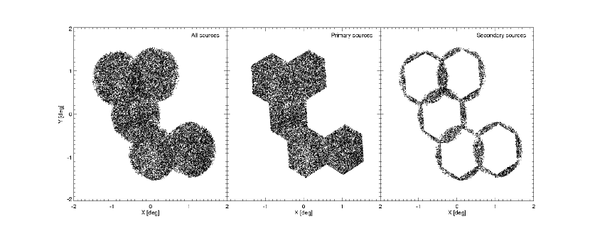
Figure 1.— Sources in a few random MIS fields shown in a tangent plane projection. The left panel shows all observed sources that are split up into primaries and secondaries seen in the middle and right panels, respectively. See text for a detailed discussion on the advantages of primaries.

Table 2GALEX Mask Flags

Bit	Value	Description
0	1	Detector bevel edge reflection
1	2	Detector window reflection
2	4	Dichroic reflection
5	32	Detector rim proximity at $R=0.59^{\circ}$

There still remains the issue of duplicated fields; grid cells that were targeted multiple times. Although these are very rare and are not intentionally part of the data releases, both AIS and MIS contain examples by accident. Our solution is to include only the longest exposure-time field per cell and reflect this in the primary flag of all sources in the other fields; see details in § 4.1.

Primaries make up roughly 65% of the AIS or MIS detections. All numbers quoted regarding these two surveys hereafter refer to primary sources, unless stated otherwise. We do not define the primary resolution for other surveys, as they do not follow the same (or any) systematic pattern on the sky.

2.2. Censoring Known Artifacts: Masks

The GALEX photometric pipeline not only produces the calibrated images but also builds models for potential artifacts based on the pointing of the telescope and other variables. These models are represented as flagmap images whose values describe the potential issue at that particular pixel position. Table 2 describes the four separate layers that the different flag values indicate.

We use these maps to censor our datasets, and mask out the artifacts. Our approach is again a geometrical one in order to maintain a clear understanding of the angular selection function. We use the Hoshen & Kopelman (1976) percolation algorithm to identify the clusters of contiguous pixels in the flagged regions, and these islands are then grown by a pixel to ensure that the final representation of the boundary encloses the original shape. We derive the convex hull of every island separately in pixel coordinates. These are polygons that accurately capture the outlines of these problematic shapes. With the world-coordinate transformations of the images (WCS; Greisen & Calabretta, 2002; Calabretta & Greisen, 2002) in hand, we then convert the enclosing pixel polygon into a spherical region that describes the censored area on the celestial sphere. We call these masks.

The artifact flags are also stored for all detections and for both bands; the properties are called fuv_artifact and nuv_artifact consistently in all data release products including the FITS files and the database servers.

2.3. Sky Coverage

It is absolutely vital to have a precise geometric representation of the surveys’ sky coverage, and our primary designation is a great first step in establishing the formal description of the exact footprint. The hexagon-like cells of the primaries are simple spherical polygons described by a half dozen (R.A., Dec) points. The union of all these polygons is a good first approximation of the sky coverage, but not good enough.

So far, we have not used anywhere the information where the telescope was actually pointing when the field was observed, only what cell the survey was targeting with that exposure. In an ideal world these two would be the same, but in practice they are not and sometimes the offsets are quite significant. We need to include an additional constraint on top of the primary cell definition that describes the field of view. For GALEX, this is a circle around the true field center (avaspra, avaspdec) with a nominal field radius of 36′ or could be a more conservative 30′ threshold. In Figure 2 we show the MIS and AIS (primary) coverage in a randomly chosen small patch of the sky using a stereographic projection centered on $(\alpha,\delta)=(0^{\circ},10^{\circ})$. The footprint in the left (right) panel assumes a 36′ (30′) radius field of view. Note that some of the SkyGrid cells have partial coverage even with the 36′ radius, where the pointing of the field was considerably off from the targeted position.

We use a generic mathematical framework (Szalay et al., 2005) and a light-weight but high-performance spherical geometry library to express all these in a uniform way by using the halfspace, convex, region concepts detailed in Budavári et al. (2008). For every field, we intersect the spherical polygon of the primary cell with the small circle constraint of the field of view, and take a union of all fields to arrive at the exact footprint description. The GALEX sky coverage is available online on the US National Virtual Observatory’s (NVO; Graham et al., 2008) Footprint Service (Budavári et al., 2007). A screenshot of the web site is shown in Figure 3, where the GR3 AIS and MIS footprints are compared to the SDSS DR6 photometric sky coverage in an Aitoff projection.

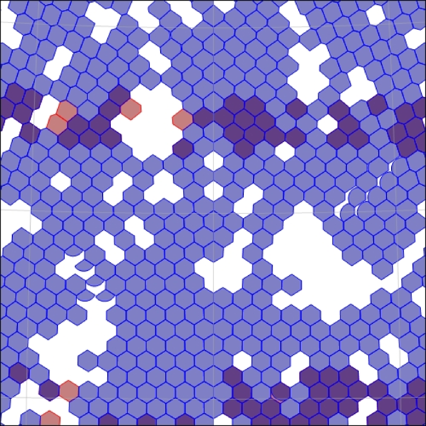
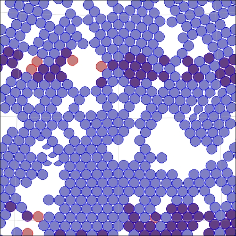
Figure 2.— These closeups of MIS and AIS primary cells (shown in red and blue, respectively) illustrate the level of details in the sky coverage representation in a stereographic projection at a randomly chosen position on the sky; $(\alpha,\delta)=(0^{\circ},10^{\circ})$. On the left, the fields are limited by the nominal 36′ radius circle around the field center; on the right, the limit is a more conservative 30′ radius. Note some of the cells have partial coverage even in the left panel, where the pointing of the field was considerably off from the targeted position.

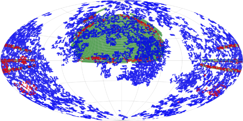
Figure 3.— Footprints of the SDSS (green), GALEX AIS (blue) and MIS (red) imaging surveys, using an Aitoff projection of the equatorial J2000 system centered on the usual $(\alpha,\delta)=(180^{\circ},0^{\circ})$ coordinates.

On top of the footprint, one needs to consider the masks; see § 2.2. The masks are defined per field but may very well extend beyond the limits of the primary cell. The secondary parts of the masks need not be applied on the primary catalog, so one needs to intersect the masks with the primary cells of their corresponding fields and use that to censor the sources.

The above mathematical representation of the footprint and the masks not only enables fast filtering of random and simulated source catalogs but also provides an exact (analytic) calculation of the area for a given polygon, which is important for essentially all statistical studies, e.g., the normalization of luminosity functions.

2.4. Merged Catalogs

The GALEX photometric pipeline processes the FUV and NUV images separately. Having run a custom, modified version of the Source-Extractor (a.k.a. SExtractor; Bertin & Arnouts, 1996) on both bands separately, the pipeline then attempts to merge the detections into sources that are stored in the MCAT FITS files.

Naturally the sources are not exactly at the same position in the two bands, hence the pipeline relies on the distance between the FUV and NUV detections and implements a hard cutoff at three arcseconds of separation, i.e., detections that are closer than 3” are merged into a single source (if they meet the eligibility criteria in Morrissey et al., 2007), otherwise left alone as single-band detections.

For the merged objects, all FUV and NUV measurements are propagated along with the measure separation. Since the NUV detections are typically much higher signal-to-noise ratio than the FUV, where the precision is often limited by the small number of observed photons, the merged object carry the position of the NUV detections by default. While this a sensible choice, one needs to be aware of the fact when pinning down geometrical constraints.

3. Cross-Identification of Sources

Table 3Number of matched sources by SDSS types

Classifier	Type	AIS	MIS
Photo	galaxy	4,542,255	2,651,799
	star	2,973,395	1,059,731
Spectro	galaxy	132,968	37,060
	star	20,930	4,284
	quasar	30,860	6,419
	high-$z$ quasar	524	126

Note. — Numbers are given for one-to-one matches of primary sources in both GALEX and SDSS.

The cross-identification of sources in various catalogs is fairly complicated in general. One needs a good understanding of the astrometry of the observations involved and their sky coverage. With the footprint descriptions in hand, one can decide whether a missing counterpart is truly a dropout or if that part of the sky was just simply not covered by the other observation. Based on the astrometric precisions one can assign a probability to a set of detections in separate catalogs that determines whether they belong to the same object. Budavári & Szalay (2008) introduced a Bayesian approach to the matching problem, and showed that for the usual astrometric model, the spherical normal distribution (Fisher, 1953), the problem can be analytically integrated. The observational evidence for a set of sources being the same object is calculated as a function of their separations and, of course, the astrometric precisions.

3.1. SDSS Versus GALEX

The SDSS data releases are accompanied by concise descriptions on the Project’s web site as well as refereed science papers, and the latest 6th Data Release we focus on here is no exception (DR6; Adelman-McCarthy et al., 2008). We applied only a few modifications to correct for some minor flaws in DR6 involving the primary resolution of a handful of sources, i.e., duplicate primaries in Stripe 36 and extra fields outside the primary footprint in Stripes 38 and 44, and incorrect SkyVersion in some of the mask identifiers. These issues were discovered after the catalogs went public, and while the upcoming new catalogs will not have these issues, the official DR6 dataset was frozen with the release.

When the probabilistic cross-identification methodology is applied to the SDSS and GALEX cases with the nominal $\sigma=0.1\arcsec$ (Pier et al., 2003) and $0.5\arcsec$ (Morrissey et al., 2007) accuracies, respectively, we find the separation limits as a function of the probability threshold. For matching GALEX sources to SDSS, the Bayes factor becomes unity at less than 4″. This does not mean that one has to accept all matches within 4″, but rather it provides a safe search radius for selecting candidates. This limit is approximately 5″ when matching GALEX to itself. Also, we find that for MIS the probability limit of 50% is at around 3″.

Figure 4.— Distributions of pairwise distances for GALEX-SDSS primary matches: one-to-one matches (solid lines), one-to-two matches (dashed line) and one-to-many matches (dotted lines). These distribution are plotted for the AIS (thin red) and MIS (thick blue) surveys.

Table 4GALEX-SDSS Quick Facts

	AIS	CAI	DIS	GII	MIS	NGS
Area of Intersection	3645.8	10.0	70.6	132.6	598.1	104.6
Number of GALEX Fields	4748	9	79	130	786	105
Number of Matches	9,463,978	$\cdots$	$\cdots$	$\cdots$	4,525,588	$\cdots$

Motivated by the analytic results, we found the candidate sources in the GALEX merged catalogs and the SDSS dataset by accepting the separation threshold of 4″. The matching is done entirely inside the relational database engine (SQL Server) that holds the GALEX and SDSS science archives using advanced indexing schemes to make it not only feasible but fast (Gray et al., 2006; Nieto-Santisteban, 2008). The generated slim table that connects the sources is essentially a many-to-many mapping, where most GALEX sources have only one SDSS counterpart but other combinations also occur frequently. In Table 3 we list the number of one-to-one GALEX-SDSS matches for spectroscopically confirmed stars, galaxies and quasars (SpecClass), as well as broken down by the SDSS star/galaxy separation (Type), which is based on profile fitting. The distributions of pairwise distances are shown Figure 4 for the AIS and MIS surveys. The distribution is slightly broader for the AIS matches compared to the MIS case, which is due to the lower signal-to-noise ratio that yields lower accuracy, cf. measurements in Morrissey et al. (2007).

Table 4 summarizes the basic properties of the associations. We enumerate the number of fields in the various GALEX surveys that overlap with SDSS and the number of sources within. In addition we also list the analytic area calculations of the interesections.

3.2. Visual Inspection

To visually check the GALEX-SDSS cross-identifications, and to compare UV to optical imaging of the sources in general, we developed a new online tool that displays the false-color images of the two surveys side by side. Our Image Cutout is available for the public. The web application programmatically accesses the SDSS cutout service on the SkyServer and displays that image without modification next to the GALEX image. The GALEX mosaics combine all information in the FUV and NUV images to provide the most detail. The brightness of the pixels is a function of the signal-to-noise ratios of the two UV bands added in quadrature ($\chi^{2}$ image; Szalay et al., 1999). The mapping is the asinh() function first introduced for the SDSS magnitudes (Lupton et al., 1999) that behaves like the logarithm in the classic magnitudes for bright sources but becomes linear for small fluxes. The color in each pixel encodes the ratio of the FUV to the NUV fluxes. We build the cumulative distribution of this ratio, suitably normalized in order to span the entire color palette. This distribution is then fitted by an analytical function using an atan() function. The Hue value in the HSV color space is then mapped from this fit the given FUV to NUV ratio.

Table 5Number of AIS matches by association

GALEX SDSS	1	2	Many
1	7,522,205	1,213,972	125,423
2	507,656	83,657	7,953
Many	2,598	455	59

Table 6Number of MIS matches by association

GALEX SDSS	1	2	Many
1	3,712,815	525,924	40,497
2	215,509	28,647	1,962
Many	200	29	5

The number of one-to-two (one GALEX to two SDSS) matches increases slowly with distance, which is the expected trend for random associations. The one-to-many cases may occur for various reasons: at bright magnitudes, because of shredding in SDSS, and at faint magnitudes due to objects blending in GALEX. The fraction of one-to-two (one-to-many) matches depends on the UV magnitude: it is roughly constant at 20% (5%) up to FUV=19 and decreases to 10% (0%) at FUV=24. For NUV-selected sources, the fraction is fairly constant at 15% (5%) up to NUV=18 and then decreases to 10% (0%) at NUV=24. In Tables 5 and 6, we enumerate the frequency of the various cases.

The other large component in the contingency matrices is the two-to-one matches, where there are two GALEX detections for every SDSS source. Our visual inspection of a large number of these cases unravels a peculiar fact: most of these associations, roughly 85%, have GALEX sources, where one out of the two is detected in the NUV only and the other in only the FUV. This suggests the possibility that all these detections are, in fact, from the same source but they were not merged in the pipeline because they were either not eligible to be merged by not meeting the signal-to-noise ratio limit, or their distances are greater than the 3″ limit.

Figure 5.— Distributions of pairwise distances for GALEX-GALEX primary matches: one-to-one matches (solid lines), one-to-two matches (dashed lines) and one-to-many matches (dotted lines). These distribution are plotted for the AIS-AIS (thin red) and MIS-MIS matches (thick blue). The break at 3″ is due to the fact that FUV and NUV sources at smaller separations are already merged by the pipeline prior to our cross-identification.

3.3. Revisiting GALEX Band-Merging

We performed the cross identification of the GALEX sources to themselves (excluding the identities) with a search radius of 5″ using the nominal positions, (ra, dec). This limit is again motivated by the Bayesian analysis, and should provide a safe margin to elect all candidates. The pairwise distance distributions of primaries are shown in Figure 5. We see a sharp break at 3″, the limit of the official band merging. At smaller separations than the break, there can be sources that were very close to the SNR threshold: although they made the detection limit of SExtractor, they were not eligible to be merged. These two thresholds are both roughly at around $2\sigma$ but not exactly the same in the two applications. Alternatively these could be cases where one of the sources in the pair are already merged with some another source. We find that the latter is not the case. In fact, the whole histogram is dominated entirely by NUV/FUV only detections. Below the break, the FUV fluxes are essentially in the noise. Above the 3″ separation, it is again FUV/NUV only detections of any signal-to-noise ratio. Our statistics are also in accord with the visual inspection described in the previous section.

Figure 6.— Color-magnitude diagrams for MIS pipeline-merged sources (thin blue in top panels), random FUV-NUV associations for reference (thin black in bottom panels) and merged sources from the GR3-GR3 cross-identifications (thick red). The left and right panels show the results for pairs with smaller and larger than 3″ separations. The insets on the right in all panels show the normalized histograms of the corresponding samples.

The census of the merged FUV-NUV pairs inside and beyond the official 3″ separation limit can only be done systematically in a statistical way due to their large numbers. Our approach is to assume that the associations are correct and study their properties, namely the UV color-magnitude diagram, to look for inconsistencies. We divide the sample into two subsets based on the separations (greater/less than 3″) as the two samples are expected to have different properties, and compare their distributions to a couple of reference sets. The first is the list of the merged sources produced by the GALEX pipeline, and the other is an artificial dataset, where one randomly shuffles the NUV-FUV associations. These two distributions are naturally quite different. If the distribution of the matched detections follows the trends seen in the pipeline data, we can be confident that they are typically good associations, and if they are more similar to the randomized dataset, they are mostly noise. Figure 6 shows the results of these comparisons in four panels. Each panel contains an inset on the left with the color-magnitude diagram and the normalized color histogram on the right. The left panels illustrate the small separation subsample, and the right panels the pairs with large distances. The top and bottom two panels, compare these distributions to the different reference sets: pipeline on top, the randoms below. We see that the associations with smaller than 3″ separations look more like the randoms, although the asymmetric shape of the color histogram suggests that there are real objects in the mixture, as well. Knowing that these are very low signal-to-noise detections, this result is what one would expect. On the right, we see that on the other side of the 3″ break the sources look very much like the pipeline colors. Since we elected the 5″ matching radius to be a safe cut, it seems odd at first that, in fact, most of these associations with these larger separations have meaningful UV colors. The implication of these results is that the astrometric precision is less accurate than the nominal $\sigma=0.5\arcsec$. We find independently that the limitation of the positional accuracy is set by the low photon counts in the FUV detectors, which is being studied and will be better assessed for the upcoming data releases. In Figure 7 we look at the positional differences between GR3 and DR6 primaries, using only one-to-one matches, to quantify the accuracy as a function of the NUV magnitude. For this measurement we selected a clean subsample of SDSS point sources. In accord with our expectations, we see that the accuracy gets worse with the magnitude and it is often higher than 0.5″.

Since the colors of the associations at these larger separations out to 5″ statistically prove to be physical, one can safely include large fraction of these extra merged sources that are quite significant in number. The increase in the size of the merged catalog is up to 12% for MIS, and even higher, due to the lower signal-to-noise ratios, for AIS up to 26%.

In Figure 8 we plot the same four panels for GALEX associations that share a common SDSS object. While the basic characteristics of the figures are essentially identical to the previous, one sees a difference in the wings of the color distributions, which are slightly tilted away from the artificial random colors. Using this extra constraint promises to improve the detection limit when desired.

Figure 7.— Precision of the GR3 astrometry in the MIS (left) and AIS (right) as a function of the apparent NUV magnitude. The precision of GALEX detections is measured by the median angular separations from the corresponding SDSS DR6 point sources. Only one-to-one match primaries are considered.

We estimate the fraction of extra merged sources with separations larger than 3″ that have similar properties than pipeline sources within the UV color magnitude-diagram. To that aim, we assume that the distribution of the extra merged sources is a linear combination of pipeline and random data. The overall fraction of extra merged sources similar to pipeline data is $\sim 0.6$ if we consider only GALEX associations. Using the associations that share a common SDSS object yields a larger fraction: $\sim 0.65$. The results depend on magnitude, as most of the objects with pipeline-like colors are fairly faint; for objects with 20$<$FUV$<$22, the fraction is 0.65 (0.7 with SDSS constraint); for fainter objects, 22$<$FUV$<$24, the fraction increases to 0.7 (0.8 with SDSS constraint).

4. Defining the Catalogs

Understanding the GALEX reduction pipeline and the properties of the extracted source catalogs is crucial for working with the data. We use the GALEX dataset as published by the Multimission Archive at the Space Telescope Science Institute (MAST) and augment the database with auxiliary tables and properties. The additions include tables to describe the geometry of the SkyGrid in form of the database table SkyGridV2 and the information to link the cells to the GALEX fields via the GridID column in the table PhotoExtract. Some of the changes had been propagated back to the official MAST site but the full update is expected in early 2009 along with the new GALEX and SDSS releases (GR5 and DR7) for which this paper also serves as a guidebook and documentation.

Due to the large overlap between the GALEX and SDSS sky coverage, it is best to keep both datasets in the same logical framework to perform meaningful selections in reasonable times. MAST is expected to start serving the associations early next year. To accommodate the typical science queries, we will provide early access to the GR3 and DR6 cross-match catalog via the CasJobs site hosted at The Johns Hopkins University. The site utilizes technologies developed for federating archives within the National Virtual Observatory (NVO).

4.1. Working with Primaries

As discussed in § 2.1, the use of primaries is very advantageous since this collection includes every source only once. The complicated geometrical selection criteria based on the SkyGrid cells should not discourage their usage. Every GALEX source in the database has a flag called Mode that provides the result of the primary resolution. The value of this property is set to 1 for all primaries and to 2 for secondaries. Sources that are not in AIS or MIS will have a value of 0. By definition, any other values signal a problem. Figure 9 illustrates an SQL request that retrieves MIS primaries that are seen in both FUV and NUV (merged by the photometric pipeline) if they are within 30′ from the center of the field. Note the field center is not the center of the SkyGrid cell but the position encoded in the (RA, Dec) coordinates (avaspra, avaspdec).

A simple and useful test is to look for duplicate fields. Since the primaries are defined field-by-field, incidental multiple exports of the same part of the sky would again result in double-counting of certain sources. The query in Figure 10 finds the problematic cells for AIS and MIS. In the catalog up to GR3, both contain a field each that was exported twice and one of those fields, preferably with the less exposure time, should be excluded. Instead of removing the fields from the data release, we simply flip a bit of the Mode to exclude these sources from our statistical samples; the values will be 5 and 6.

While we are looking at the fields, let us quickly also determine which are the fields that are covered by both AIS and MIS. The subsamples within them are invaluable for cross checks and studies of the limitations. In Figure 11 we show an SQL command that compares the FUV exposure times for the resulting fields.

4.2. Working with Associations

We provide the cross-identification of all GALEX sources to themselves. The links stored in the table xSelf not only enable quality assurance and diagnostic tests, but also deliver the missing merged sources at separations larger than the 3″ limit in the GALEX pipeline out to 5″. The query in Figure 12 emulates the pipeline merging. Here one picks the pairs where one is NUV only detection (Band=1) and the other is FUV only (Band=2) and only requires the NUV detection to be primary, as it is the accepted position for the merged source in the pipeline.

The GALEX-SDSS DR6 associations are stored in the table xSdssDR6, which again represents many-many mapping between the sources. We also introduce tables where the sources are grouped by GALEX and SDSS identifiers and store the number of matches for each, see tables starting with xGroup. Figure 13 shows an SQL query that counts the number of one-to-one matches, where both SDSS and GALEX sources are primaries and breaks the numbers down by the SDSS object classification.

Figure 8.— Same as Figure 6 for GALEX associations that share a common SDSS counterpart.

SELECT ObjID, FUV_Mag, NUV_Mag
FROM PhotoObjAll o
    JOIN PhotoExtract e ON e.PhotoExtractID = o.PhotoExtractID
WHERE e.MpsType = ’MIS’
    AND o.Mode = 1 -- i.e., primary
    AND o.Band = 3 -- both bands (1:NUV, 2:FUV)
    AND o.FoV_Radius < 0.5

Figure 9.— An example query in SQL to retrieve all GALEX MIS primaries within 30′ of the field centers that have both FUV and NUV measurements merged by the photometric pipeline. The Transact-SQL keywords are typeset in capital letters; for table and column names, we use the conventional camel case spelling.

With the formal description of the GALEX footprint in hand, it is straightforward to look for dropouts, where the SDSS source is missing in GALEX. We achieve this by first assigning every SDSS source to a SkyGrid cell and then selecting the cells that were actually observed in the given survey. The table SdssDr6inMisPrimary contains all the SDSS sources that are in the MIS footprint along with the distance to the actual field center. Figure 14 illustrates the query where the crossmatch table is used to search for SDSS galaxies close to the field center, $d<0.5^{\circ}$, without a counterpart.

4.3. Revised band-merging

We now combine the above key elements of sample selection into a real-life example of creating a catalog of primaries with detections in both bands using the extra associations discussed above, i.e., the FUV-, NUV-only matches at larger angular separations than the official pipeline cutoff. We propagate the basic quantities of GALEX measurements along with links to the SDSS associations, where available. Figure 15 illustrates the SQL command that defines the final catalog; the union of the three sub-queries. These are conceptually really only two: the pipeline merged sources (Band=3) and the one-to-one GALEX matches (Band=1 to Band=2). The third part is simply a result of the fact that the match table xSelf is not symmetric by construct to save storage space and is essentially identical to the previous one except for the order of the ObjIDs in the join criteria.

SELECT MpsType, GridID, COUNT(*)
FROM PhotoExtract
WHERE MpsType IN (’AIS’,’MIS’)
GROUP BY MpsType, GridID
HAVING COUNT(*) > 1
-- AIS   2350  2
-- MIS  21884  2

Figure 10.— Look for SkyGrid cells in AIS and MIS that were observed multiple times and need to be resolved for a clean sample to avoid duplicates.

SELECT mis.PhotoExtractID AS MisID, mis.FExpTime AS MisFExpTime,
       ais.PhotoExtractID AS AisID, ais.FExpTime AS AisFExpTime
FROM PhotoExtract mis
    JOIN PhotoExtract ais ON ais.GridID = mis.GridID
WHERE mis.MpsType = ’MIS’ and ais.MpsType = ’AIS’
-- 809 fields

Figure 11.— Look for fields that have been observed in both AIS and MIS.

SELECT e1.MpsType, COUNT(*) as Number
FROM xSelf x
    JOIN PhotoObjAll o1 ON o1.ObjID = x.ObjID
    JOIN PhotoObjAll o2 ON o2.ObjID = x.MatchID
    JOIN PhotoExtract e1 ON e1.PhotoExtractID = o1.PhotoExtractID
    JOIN PhotoExtract e2 ON e2.PhotoExtractID = o2.PhotoExtractID
        AND e1.PhotoExtractID = e2.PhotoExtractID
WHERE x.Distance BETWEEN 3 AND 5
    AND e1.MpsType IN (’AIS’, ’MIS’)
    AND (    (o1.Band = 1 AND o2.Band = 2 AND o1.Mode = 1)
          OR (o1.Band = 2 AND o2.Band = 1 AND o2.Mode = 1)
        )
GROUP BY e1.MpsType

Figure 12.— SQL query that counts the number of NUV-only primaries in AIS and MIS that are matched to FUV-only detections in the same field with separations between 3″ and 5″.

SELECT x.MatchType, COUNT(*)
FROM xSdssDr6 x
    JOIN xGroupMIStoSdssDr6Primary gs ON gs.ObjID = x.ObjID
    JOIN xGroupSdssDr6toMISPrimary sg ON sg.MatchID = x.MatchID
WHERE x.Mode = 1 AND x.MatchMode = 1 -- both primaries
    AND gs.N = 1 -- only 1 SDSS match for GALEX source
    AND sg.N = 1 -- only 1 GALEX match for SDSS source
GROUP BY x.MatchType -- e.g., 3:Galaxy, 6:Star

Figure 13.— Returns the number of one-to-one matches of GALEX and SDSS primaries broken down by the SDSS photometric type classification.

SELECT COUNT(*)
FROM SdssDr6inMisPrimary s
    LEFT OUTER JOIN xSdssDr6 x ON x.MatchID = s.ObjID
WHERE s.Type = 3 -- i.e., galaxy
    AND s.Distance < 0.5 -- from the field center
    AND x.ObjID IS NULL -- no match

Figure 14.— Returns the number of SDSS primaries in the MIS footprint that are closer to the field center than 30′ but have no GALEX counterparts, a.k.a. dropouts.

We select the most common properties sufficient for many scientifically interesting queries but note that any other attributes are also easily selected by joining the result of this query with the original PhotoObjAll table. The columns we choose to propagate are the following: (1) MpsType that takes the values of AIS and MIS, (2) the field identifier PhotoExtractID, (3-4) the identifiers of the FUV and NUV observations, which are the same for the merged objects, (5-6) NUV position, (7-8) magnitudes, (9) angular separations in arcseconds between the FUV and NUV detections, and (10) the identifier of the SDSS primary associations and (11) their distances in arcseconds, where available. The first query simply picks GALEX primaries with both bands but the anatomy of the following is more complicated: We use the aforementioned xSelf table to link NUV-only primaries to FUV-only sources within the same fields that are farther than 3″. Note that because the we elect the NUV coordinates to be the position of the merged source following the pipeline strategy, we do not require the FUV-only source to be a primary. We also ensure that only one-to-one GALEX matches are used, which is essentially everything. The final size of the AIS and MIS two-band catalogs grow from 2,634,974 to 3,819,307 and 1,549,355 to 1,988,882, respectively.

Another approach to improve on the colors of the sources is to use a separate set of FUV fluxes from the GALEX pipeline: The FUV flux within the NUV aperture is also published in the catalog called fd-ncat, whose parameters are also found in the PhotoObj table. For the DIS catalogs, where the confusion becomes an issue, there is a new algorithm being developed to use optical and/or NUV prior information on the positions. The potential problem with the fd-ncat measurements arises when the NUV and FUV positions are significantly different and the NUV aperture encloses only part of the FUV object, which yields typically smaller FUV fluxes than the actual. This could considerably affect techniques that strongly rely on the color, such as the FUV dropout selection of the Wiggle-Z project (Glazebrook et al., 2007).

5. Summary

We presented a detailed study of the GALEX photometric catalogs. Our discussion focused mostly the AIS and MIS datasets and their properties. We define the primary area of the fields to resolve duplicates in overlapping fields and the sky coverage. We also derived masks that are stored along with the sources in spherical polygons. We performed the cross-identification of the GALEX GR2+3 and SDSS DR6 sources and indicated issues with multiple matches that often point toward unmerged GALEX detections that are only seen in the NUV and in the FUV. We found that merging these detection can be safely done out to 5″ separations, which also implies that the nominal $\sigma=0.5\arcsec$ astrometric precision is somewhat optimistic. We made the cross-match catalogs available to the general public in the form of a SQL Server database engine and showed various examples of SQL queries to not only access the data but to extract clean catalogs for scientific analysis.

SELECT e.MpsType, o.PhotoExtractID,
    o.ObjID as FuvObjID, o.ObjID as NuvObjID,
    o.RA, o.Dec, o.Fuv_Mag, o.Nuv_Mag,
    60*dbo.fDistanceArcMinEq(Nuv_RA,Nuv_Dec,Fuv_RA,Fuv_Dec) as Separation,
    gs.MatchID as SdssObjID, gs.Distance as Distance
FROM PhotoObjAll o
    JOIN PhotoExtract e ON e.PhotoExtractID=o.PhotoExtractID
    LEFT OUTER JOIN xSdssDR6 gs
        ON gs.ObjID = o.ObjID AND gs.MatchMode = 1
WHERE Band = 3 AND o.Mode = 1 -- Primaries with both bands

UNION ALL

SELECT en.MpsType, n.PhotoExtractID,
    f.ObjID as FuvObjID, n.ObjID as NuvObjID,
    n.RA, n.Dec, f.fuv_mag as FUV_mag, n.nuv_mag as NUV_mag,
    gg.Distance as Separation,
    gs.MatchID as SdssObjID,
    gs.Distance as Distance
FROM xSelf gg
    JOIN PhotoObjAll f ON f.ObjID = gg.ObjID
    JOIN PhotoObjAll n ON n.ObjID = gg.MatchID
    JOIN PhotoExtract ef ON ef.PhotoExtractID = f.PhotoExtractID
    JOIN PhotoExtract en ON en.PhotoExtractID = n.PhotoExtractID
        AND ef.PhotoExtractID = en.PhotoExtractID
    JOIN xGroupAMIStoAMIS g1 ON g1.ObjID = n.ObjID
    JOIN xGroupAMIStoPrimary g2 ON g2.ObjID = f.ObjID
    LEFT OUTER JOIN xSdssDR6 gs
        ON gs.ObjID = n.ObjID AND gs.MatchMode = 1
WHERE gg.Distance BETWEEN 3 AND 5
    AND n.Band = 1 AND f.Band = 2 AND n.Mode = 1
    AND g1.N = 1 AND g2.N = 1 -- One-to-one GALEX match

UNION ALL

SELECT en.MpsType, n.PhotoExtractID,
    f.ObjID as FuvObjID, n.ObjID as NuvObjID,
    n.RA, n.Dec, f.fuv_mag as FUV_mag, n.nuv_mag as NUV_mag,
    gg.Distance as Separation,
    gs.MatchID as SdssObjID,
    gs.Distance as Distance
FROM xSelf gg
    JOIN PhotoObjAll f ON f.ObjID = gg.MatchID
    JOIN PhotoObjAll n ON n.ObjID = gg.ObjID
    JOIN PhotoExtract ef ON ef.PhotoExtractID = f.PhotoExtractID
    JOIN PhotoExtract en ON en.PhotoExtractID = n.PhotoExtractID
        AND ef.PhotoExtractID = en.PhotoExtractID
    JOIN xGroupAMIStoAMIS g1 ON g1.ObjID = n.ObjID
    JOIN xGroupAMIStoPrimary g2 ON g2.ObjID = f.ObjID
    LEFT OUTER JOIN xSdssDR6 gs
        ON gs.ObjID = n.ObjID AND gs.MatchMode = 1
WHERE gg.Distance BETWEEN 3 AND 5
    AND n.Band = 1 AND f.Band = 2 AND n.Mode = 1
    AND g1.N = 1 AND g2.N = 1 -- One-to-one GALEX match

Figure 15.— Revised band-merging in SQL; see text for details.

In this analysis, we started with the official GALEX pipeline sources, because it is the reference dataset that all studies rely on. Some of these results have been already incorporated in the next GR4 release, which should show improvements and will have to be studied further. Our immediate future work is to treat the GALEX FUV and NUV detections as separate catalogs for the purpose of cross-identification with SDSS and instead of performing a 2-way join between GALEX and SDSS, where GALEX catalog is already the result of a previous 2-way match. This new 3-way cross-matching of the SDSS and the two GALEX bands will be done using the probabilistic formalism of Budavári & Szalay (2008), however, for this next generation analysis one will need a better understanding of the astrometry of the GALEX sources, especially in the FUV, where the measurements are limited by the small number of photons.

References

- Adelman-McCarthy et al. (2008) Adelman-McCarthy, J. K., et al. 2008, ApJS, 175, 297
- Bertin & Arnouts (1996) Bertin, E., & Arnouts, S. 1996, A&AS, 117, 393
- Bianchi et al. (2005) Bianchi, L., et al. 2005, ApJ, 619, L27
- Bianchi et al. (2007) Bianchi, L., et al. 2007, ApJS, 173, 659
- Budavári et al. (2007) Budavári, T., et al. 2007, in ASP Conf. Ser., Vol. 376, Astronomical Data Analysis Software and Systems (ADASS) XVI, eds. R. A. Shaw, F. Hill, & D. J. Bell (San Francisco: ASP), p.559
- Budavári et al. (2008) Budavári, T., et al. 2008, in ASP Conf. Ser., Vol. 382, The National Virtual Observatory Book, eds. M. J. Graham, M. J. Fitzpatrick, & T. A. McGlynn (San Francisco: ASP), p.75
- Budavári & Szalay (2008) Budavári, T., & Szalay, A. S. 2008, ApJ, 679, 301
- Calabretta & Greisen (2002) Calabretta, M. R., & Greisen, E. W. 2002, A&A, 395, 1077
- Fisher (1953) Fisher, R., 1953, Proceedings of the Royal Society of London, Series A, Mathematical and Physical Sciences, Vol. 217, No. 1130., pp.295–305
- Giavalisco (2002) Giavalisco, M. 2002, ARA&A, 40, 579
- Glazebrook et al. (2007) Glazebrook, K., et al. 2007, ASP Conf. Ser., Vol. 379, Cosmic Frontiers, eds. N. Metcalfe & T. Shanks, 72
- Graham et al. (2008) Graham, M. J., Fitzpatrick, M. J., & McGlynn, T. A., et al. 2008, ASP Conf. Ser., Vol. 382, The National Virtual Observatory: Tools and Techniques for Astronomical Research, eds. M. J. Graham, M. J. Fitzpatrick, & T. A. McGlynn (San Francisco: ASP)
- Gray et al. (2006) Gray, J., Nieto-Santisteban, M. A., & Szalay, A. S. 2006, Microsoft Research Technical Report, MSR-TR-2006-52
- Greisen & Calabretta (2002) Greisen, E. W., & Calabretta, M. R. 2002, A&A, 395, 1061
- Hoshen & Kopelman (1976) Hoshen, J., & Kopelman, R. 1976, Phys. Rev. B, 14, 3438
- Kennicutt (1998) Kennicutt, R. C., Jr. 1998, ARA&A, 36, 189
- Lupton et al. (1999) Lupton, R. H., Gunn, J. E., & Szalay, A. S. 1999, AJ, 118, 1406
- Martin et al. (2005) Martin, D. C., et al. 2005, ApJ, 619, L1
- Morrissey et al. (2007) Morrissey, P., et al. 2007, ApJS, 173, 682
- Nieto-Santisteban (2008) Nieto-Santisteban, M. A. 2008, PhD thesis, in preparation
- Pier et al. (2003) Pier, J. R., et al. 2003, AJ, 125, 1559
- Schlegel et al. (1998) Schlegel, D. J., Finkbeiner, D. P., & Davis, M. 1998, ApJ, 500, 525
- Seibert et al. (2005) Seibert, M., et al. 2005, ApJ, 619, L23
- Steidel et al. (1995) Steidel, C. C., Pettini, M., & Hamilton, D. 1995, AJ, 110, 2519
- Szalay et al. (1999) Szalay, A. S., Connolly, A. J., & Szokoly, G. P. 1999, AJ, 117, 68
- Szalay et al. (2005) Szalay, A. S., Gray, J., Fekete, G., Kunszt, P., Kukol, P., & Thakar, A. R. 2005, Microsoft Research Technical Report, MSR-TR-2005-123
- Voronoi (1908) Voronoi, G. 1908, J. Reine Angew. Math, 134, 198
- Wyder et al. (2007) Wyder, T. K., et al. 2007, ApJS, 173, 293
- York et al. (2000) York, D.G., et al. 2000, AJ, 120, 1579