A Class of Novel STAP Algorithms Using Sparse Recovery Technique

Abstract

A class of novel STAP algorithms based on sparse recovery technique were presented. Intrinsic sparsity of distribution of clutter and target energy on spatial-frequency plane was exploited from the viewpoint of compressed sensing. The original sample data and distribution of target and clutter energy was connected by a ill-posed linear algebraic equation and popular $L_{1}$ optimization method could be utilized to search for its solution with sparse characteristic. Several new filtering algorithm acting on this solution were designed to clean clutter component on spatial-frequency plane effectively for detecting invisible targets buried in clutter. The method above is called CS-STAP in general. CS-STAP showed their advantage compared with conventional STAP technique, such as SMI, in two ways: Firstly, the resolution of CS-STAP on estimation for distribution of clutter and target energy is ultra-high such that clutter energy might be annihilated almost completely by carefully tuned filter. Output SCR of CS-STAP algorithms is far superior to the requirement of detection; Secondly, a much smaller size of training sample support compared with SMI method is requested for CS-STAP method. Even with only one snapshot (from target range cell) could CS-STAP method be able to reveal the existence of target clearly. CS-STAP method display its great potential to be used in heterogeneous situation. Experimental result on dataset from mountaintop program has provided the evidence for our assertion on CS-STAP.

I Introduction

Space-time adaptive processing (STAP) is a signal processing technique that was originally developed for detecting slowly moving targets using airborne radars[1]. In this decade, the need for STAP to perform well in heterogeneous environments, that is, lack of (wide-sense) stationarity of the received signals with respect to range and snapshots is becoming more and more urgent[2]. In fact, the unknown clutter and interference covariance matrix should be estimated from a set of independent identically distributed (i.i.d.) target-free training data, which is assumed to be representative of the interference statistics in a cell under test. The consistency of estimator depends heavily on the stationarity of training data. In case the stationary hypothesis is violated, the performance of STAP filter based on sample covariance matrix of data from training cells will degrade dramatically. But in practical scenario, stationarity of training environment tends to disappear when terrain deviates from being flat with uniform reflectivity properties and in the presence of internal clutter motion such as tree leaves moving in the wind; On the other hand, the training data are subject to contamination by discrete scatterers or interfering targets. radar system configurations such as conformal arrays and bi-static geometries is also important factor of non-homogeneity of training data. So the stationarity is hard to be guaranteed and conventional covariance estimation methods usually could not be helpful because it is impossible to get enough ideal training data to calculate the optimal space-time filtering weight vector.

To overcome the difficulty brought by non-homogeneous clutter and interference, various methods is proposed to improve the quality of estimation of covariance matrix. Algorithms of non-homogeneity detection pay attention to how to detect and eliminate outlier in a variety of dense target environments[3][4][5][6].Methods in this context is to excise outliers from the training data and use the resulting outlier-free training data for covariance matrix estimation But most methods of outlier removal relies on full-dimension STAP processing and therefore is not suited for conditions of limited sample support. Especially when main source of non-stationarity is the great diversity of clutter reflecting characteristic in training cells, simply detecting and removing the outlier is not enough to build satisfactory STAP filter. $D^{3}$(Direct Data Domain) methods is different from conventional statistical techniques based upon the covariance matrix[7][8][9].It use data from the primary range cell only, and so bypass the problem of the required homogeneous secondary data support. Although $D^{3}$ algorithms perform well when blinking jammer are encountered, they are not as effective against the homogeneous component of the interference because they ignore all statistical information. In recent years the approach received much attention is so called knowledge based STAP[10]. Traditional STAP methods make little use of a priori knowledge such as anticipated structure of surface clutter returns and cultural information available from land-use databases and digital terrain elevation data (DTED) models[11]. On the contrary, these prior knowledge is utilized skillfully by knowledge-based STAP(KA-STAP) techniques to obtain the better effect of clutter migration. Ordinary KA-STAP methods could be roughly divided into two category[10]: Intelligent Training/Filter Selection and Bayesian Filtering/Data Pre-Whitening. Results of theoretical analysis and experimental evaluation on real data collected in research program such as MCARM or KASSPER shows that including knowledge about the operating environment in the signal processing solution offers significant detection performance gains[12][13]. It should be noticed that the exact form of prior knowledge is problem-dependent and hard to be derived. Furthermore, how to make effectively use of prior knowledge in STAP framework is still a problem worth seriously considering.

Over the last decade, the signal processing community spurred by the work of Donoho[14],Candes and Tao[15][16] pay much attention to the field of Compressed Sensing. Although the its name , especially its abbreviation ”CS”, is somewhat misleading, the essence of this active field is very natural and intuitive: If our target has some characteristic of ”Sparsity” and the process of measurement is linear, only a few of sample data is required to recover the original target exactly or approximatively. That is, if the existence of ”Sparsity” could be definite, a great deal of difficult inverse problem in electrical engineering discipline which have no effective solver in framework of traditional signal processing could be solved accurately with some powerful tools such as $L_{1}$ regularization and corresponding numerical schemes[17]. Application of Compressed Sensing on Radar is becoming more and more notable recently and much work focus on the subfield of radar imaging[18][19][20]. The basis for applicability of Compressed Sensing technique in radar imaging is there exist apparent feature of ”Sparsity” in radar reflectivity of some natural and artificial scenario, which is measuring target of radar imaging. It should be mentioned that ”Sparsity” can be revealed not only in radar echo data of time domain, but also from other viewpoint. For instance, the energy distribution of echo of clutter on spatial-frequency plane is obvious ”Sparse” because most energy of clutter concentrates on a small region typically[1]. It provides a great possibility to estimating the energy in each spatial-frequency cell directly from sample data with sparse recovery method. That is the preliminary idea of our work.

In this paper we propose a novel approach to detect the moving target in strong clutter situation using airborne radar with array antenna based on sparse processing technique. We called it CS-STAP. CS-STAP has two advantages. Firstly, data from much fewer range cells compared with conventional STAP methods based on covariance matrix estimation is used. So it can avoid in great extent the influence of heterogeneous clutter on performance of detector. In some special case, even data from one range cell is sufficient for us to detect target effectively. Secondly, our approach has ability of super-resolution. Hence the accuracy of estimation for Doppler frequency and azimuth angle of target is much higher than other covariance based STAP schemes. Ability of super-resolution presented CS-STAP capability of clearing the clutter almost completely and obtaining massive improvement on SCR. Experimental results on real data will verify the assertion above.

The paper is organized as follows. In Section II we state the basic signal model of STAP radar echo data from viewpoint of sparse recovery. In Section III we give a brief review of necessary background on Compressed Sensing and some key results will be described. In Section IV our main algorithms of detection are proposed. In Section V the performance of new methods is showed with the real data from Mountain-Top program. Section VI provides a summary of our contributions.

II Signal Model from viewpoint of Sparse Processing

Considered here is a radar system that transmits coherent pulse trains with length $L$ and samples the returns on an $N$-element uniform linear array(ULA). For each pulse, It collects $M$ temporal samples from each element receiver, where each time sample corresponds to a range cell. The temporal dimension of interest here is referred to as fast time. The collection of samples for $m$th range cell is represented by an $N{\times}L$ data matrix $X_{m}$ with elements $X_{m}(n,l)$, and the pulse dimension of interest here is referred to as slow time. echo data from all range cells is arranged into a ”Data Cube”, that is:

$$X=[X_{1},X_{2},\cdots,X_{L}]^{T},$$ (1)

which is the data basis for almost all STAP processing.

Suppose the amplitude of radar echo signal in the same coherent processing interval(CPI) from a fixed range cell, losing no generality, $k$th range cell, is stationary, that is, it doesn’t have any fluctuation, then the spatial information (azimuth angle of echo) and Doppler information (moving speed with respecting to ground) of object in observing region of radar are all contained in phase difference among elements of data matrix corresponding to that range cell.

Let $d$ equal the element spacing of ULA and place the first antenna element at the origin and designate it as phase reference. The spatial phase shift on received data at different elements is

$$\phi_{s}=[1,\exp(j2{\pi}f_{s}),\cdots,\exp(j2{\pi}\cdot(N-1)f_{s})],$$ (2)

which is usually referred as spatial steering vector, where the spatial frequency is

$$f_{s}=\frac{d}{\lambda}\cos(\theta)$$ (3)

$\lambda$ is wavelength of radar and $\cos(\theta)$ is directional cosine.

On the other hand, suppose motion of scatterer, motion of radar platform, or both lead to Doppler frequency $f_{d}$

$$f_{d}=\frac{2v}{\lambda},$$ (4)

where $v$ denotes the radical velocity component, or line-of-sight velocity. Let the first pulse in one CPI be the reference point, we obtained Doppler steering vector, the representation of Doppler phase shift on received data of different pulses in this CPI.

$$\phi_{d}=[1,\exp(j2{\pi}f_{d}),\cdots,\exp(j2{\pi}\cdot(L-1)f_{d})],$$ (5)

The Spatial-Doppler steering vector corresponding to the echo signal from a point scatterer with spatial frequency $f_{s}$ and normalized Doppler frequency $f_{d}$ is

$$\phi_{s-t}(f_{s},f_{d}) = \phi_{s}\otimes\phi_{d}$$

$$= [1,\exp(j2{\pi}f_{d}),\cdots,\exp(j2{\pi}(L-1)f_{d}),$$

$$\cdots,\exp(j2{\pi}((N-1)f_{s}+(L-1)f_{d}))],$$

where $\otimes$ denotes Kronecker product. Assume the contribution of this point scatterer in overall radar echo is $\alpha(f_{s},f_{d})$ which is a complex quantity, then the echo signal snapshot from fixed range cell can be obtain by summarizing the contribution from individual point scatterer with different spatial and Doppler frequency together,

$$r=\sum_{f_{s},f_{d}}\alpha(f_{s},f_{d})\phi_{s-t}(f_{s},f_{d}),$$ (7)

Here $r$ is a vector with the same length as $\phi_{s-t}(f_{s},f_{d})$, that is, $N{\times}L$.

Discretizing spatial and Doppler axis, we divided the spatial-frequency plane into square grids. The content in each grid represents the echo signal with spatial frequency and Doppler frequency corresponding to that grid. Then the data snapshot could be written as

$$r=\sum_{m=1}^{N_{s}}\sum_{n=1}^{N_{d}}\alpha(m,n)\phi_{s-t}(m,n),$$ (8)

where $N_{s}$ and $N_{d}$ is the number of quantization of spatial and Doppler axis respectively. Roughly speaking, they can be set arbitrarily. But we must make carefully choice on $N_{s}$ and $N_{d}$ to build practical algorithm.

It should be noted that model (8) is different from the data model proposed in [21] as follows:

$$r=\sum_{m=1}^{N_{a}}\sum_{n=1}^{N_{c}}\beta(m,n:k)\xi_{s-t}(m,n:k),$$ (9)

where $N_{a}$ and $N_{c}$ denotes the number of statistically independent clutter patches in iso-range and ambiguous ranges of $k$th range respectively. In our model, the range ambiguity is not considered and the independence of clutter in distinct grid is not required (Although it is meaningful in our algorithm design). model (8) can be written as matrix form

$$r=\Phi{x},$$ (10)

where

$$\Phi = [\phi_{s-t}(1,1),\cdots,\phi_{s-t}(1,n),\cdots,\phi_{s-t}(m,n)],$$ (11)

$$x = [\alpha(1,1),\cdots,\alpha(1,n),\cdots,\alpha(m,n)],$$ (12)

Equation (10) is the fundamental model in this paper. It has three important characteristic worthy of indicating explicitly. at first, the energy distribution of clutter and target buried in it on spatial-frequency plane could be obtained by solving linear equation (10) of unknown $x$ and known $r$ which is spatial-temporal sample data. In other words, operation of STAP is essentially a process of solving linear algebraic equation from our point of view. Secondly, the row dimension $N{\times}L$ of matrix $\Phi$ is much less than column dimension $N_{s}{\times}N_{d}$ typically. Hence equation (10) is heavily ill-posed. The number of unknown variables is much more than the number of equations. That is to say, there are infinite vectors satisfying (10) in general and some constraint should be imposed to help us to get some solution with unique feature. Thirdly, from viewpoint of STAP, the solution of (10) we are searching for is ”Sparse”. More rigorously, most of its entry are negligible and only a small portion of elements in solution vector, which represents contribution of main clutter and target, are remarkable, just as description in standard textbook of STAP [1][2]. This kind of ”Sparsity” is the basis of application of sparse recovery technique on STAP. Before our new approach is proposed, some necessary background of sparse processing will be sketched briefly.

III a brief review of necessary background on Compressed Sensing

One of the main objective of compressed sensing is seeking the solution with ”Sparse” property of heavily ill-posed linear algebraic equations (13)

$$y=Ax,$$ (13)

where $A\in{C}^{M{\times}N}$ is a ”rectangle” matrix, that is, $M{\ll}N$. Of course, equation (13) has infinite solutions if no further assumption is put forward. In many practical situation (including STAP), people focus their interests on the most ”Sparse” solution of (13), that is, the one with minimal number of ”nonzero” elements. Intuitively, the process of solving equation (13) for the most ”Sparse” solution can be transformed to so called $L_{0}$ optimization problem as follows:

$$\min\|x\|_{0},{\quad}s.t{\quad}Ax=y,$$ (14)

or more flexibly

$$\min\|x\|_{0},{\quad}s.t{\quad}\|Ax-y\|_{2}\leq\epsilon,$$ (15)

This is a combinatorial optimization problem and can be proven to be NP-hard[22]. Hence $L_{1}$ relaxation is utilized as substitution of intractable $L_{0}$ problem to find the most ”Sparse” solution. Specially, our optimization problem is changed to

$$\min\|x\|_{1},{\quad}s.t{\quad}Ax=y,$$ (16)

or more flexibly

$$\min\|x\|_{1},{\quad}s.t{\quad}\|Ax-y\|_{2}\leq\epsilon,$$ (17)

where $\|x\|_{1}=|x_{1}|+\cdots+|x_{n}|$ for $x\in{C}^{n}$. (16) is a linear programming problem essentially and can be solved effectively by popular convex optimization algorithm [23] or greedy method [24].

A important question was raised naturally: whether (14) and (16) is really equivalent? Candes and Tao defined a kind of character property for matrix $A$ named Restricted Isometry Property (RIP)[16] in order to study $L_{0}/L_{1}$ equivalence. RIP concerns with the upper and lower bound of singular values of the submatrix of $A$. In particular, for every $K\in{N}$, matrix $A$ is said to satisfy RIP of order $K$ if there exist a positive constant $\delta_{K}$, such that

$$(1-\delta_{K})\|z\|_{2}^{2}\leq\|Bz\|_{2}^{2}\leq(1+\delta_{K})\|z\|_{2}^{2},$$ (18)

for all submatrix of $A$ with dimension $M{\times}K$, where $z\in{C}^{K}$. in other words, the singular values of all submatrix of $A$ with dimension $M{\times}K$ should be restricted in interval $(1-\delta_{K},1+\delta_{K})$. Several sufficient conditions based on the value scope of RIP constant of different order have been proposed to guarantee the $L_{0}/L_{1}$ equivalence, For example[16],

$$\delta_{3K}+3\delta_{4K}<2,$$ (19)

and[25]

$$\delta_{2K}<\sqrt{2}-1,$$ (20)

Although many methods to construct matrix satisfying RIP(especially randomization method) have been brought forward[17], a lack of effective means for testing RIP and estimating RIP constant of a given deterministic matrix is still a hidden trouble for practitioners and user of compressed sensing technique[26], no exception for us. It is very hard to verify RIP of matrix used in STAP operation based on sparse recovery algorithm theoretically. So the detailed conditions for $L_{0}/L_{1}$ equivalence will not be checked in our research. Fortunately, no severe consequence was encountered generally, because simply using $L_{1}$ optimization could we find the solution of (13) with some characteristic of sparsity (although it maybe isn’t the most sparse one). That is just what we want in most cases.

IV STAP Algorithms Based On Sparse Recovery

It is easy to notice that linear equation (8) and (13) have some similarity: the row dimension of coefficient matrix is much smaller than its column dimension; the target solution is ”Sparse”. So it’s reasonable to transform equation (8) into a $L_{1}$ optimization problem to obtain the solution via convex or greedy method.

In practice, the space-time covariance matrix which is key device in framework of traditional STAP is not known in prior and needs to be estimated from the secondary data. This is just the point for which Sparse recovery method can take advantage of to improve their performance when sample support of snapshots is tiny. The reason is the contribution of point scatterer with specific spatial and Doppler frequency in overall echo could be estimated directly from snapshot by sparse recovery algorithm. So the spatial-frequency distribution of clutter could be calculated with few snapshots. Then it could be used to design effective filter to eliminate clutter and make the detection for small target possible.

Using the notation and abbreviation in Section II, let $r\in{C}^{N{\times}L}$ be sample data from single snapshot of preliminary data. In other words, the data we will deal with come from cell under test only. it may contains both clutter and target. No training cells are used in our treatment of single snapshot. From this point, the algorithm below belongs to $D^{3}$ category.

Algorithm 1 (Annihilating Filter — Single Snapshot Case)

• Choose the row dimension $N_{s}$ and column dimension $N_{d}$ for quantization grids of spatial-frequency plane.

• Form measurement matrix $\Phi$ with $N{\times}L$ rows and $N_{s}{\times}N_{d}$ columns as (11).

• Solve linear ill-posed equation $r=\Phi{x}$ to obtain $x$, the estimation of levels of echo signal with given spatial and Doppler frequency.

• Calculate the absolute value of each entry in $x$ to get $|x|=(|x_{1}|,\cdots,|x_{N_{s}{\times}N_{d}}|)$.

• Arrange the entries of $|x|$ in descend order, and estimate the index $k$ such that

  $$|x_{[1]}|>|x_{[2]}|>\cdots>|x_{[k]}|\gg|x_{[k+1]}|>\cdots>|x_{[N_{s}{\times}N_{d}]}|,$$

• Set $|x_{[1]}|=|x_{[2]}|=\cdots=|x_{[k]}|=0$ and output $|x|$.

If Clutter-Noise-Ratio(CNR) and Clutter-Signal-Ratio(CSR) are both sufficient large, then algorithm 1 can eliminate the clutter energy in sample data efficiently. we can use conventional threshold detection on the output of algorithm 1 to reveal the existence of target. Algorithm 1 is a kind of ”whiten” filter.

Except for solving linear ill-posed equation, the key step in algorithm 1 is step (5), that is, find the accurate position of clutter on spatial-frequency plane. The assumption on CNR and CSR is critical in this step. In fact, if CNR wasn’t large enough, then it was hard to find the correct index $[k]$ that can separate clutter from noise. This oracle has an analogy to that of standard MUSIC algorithm for super-resolution spectral estimation, where the right separation of signal subspace and noise subspace relies on finding the index where the eigenvalues of sample covariance matrix with descend order have a abrupt change. if SNR wasn’t large adequately, eigenvalues would change gradually and the performance of estimator of noise subspace degraded dramatically. Hence MUSIC algorithm will become invalid. Here the problem is alike. Secondly, if CSR, instead of CNR, is too small, the target is easy to be taken in mistake as part of clutter and be removed from data by Annihilating operation. On the other hand, because only one data snapshot is used and there is no any integration in algorithm 1, the noise receives no suppress and the algorithm is statistically unstable.

To increase CNR and improve the statistical stability of algorithm 1, integration of multiple data snapshots with respect to different range cells is added. It should be emphasized that although data from training cells are used in this algorithm, the necessary sample support is much smaller than that of standard STAP filter based on covariance matrix in practice.

Suppose sample support for our algorithm is $K$, Let $r^{(i)}$ be $i$th snapshot from training cell, $i=1,2,\cdots,K$, $r^{[T]}$ be snapshot from testing cell, then we have

Algorithm 2 (Annihilating Filter — Multiple Snapshots Case)

• Choose the row dimension $N_{s}$ and column dimension $N_{d}$ for quantization grids of spatial-frequency plane.

• Form measurement matrix $\Phi$ with $N{\times}L$ rows and $N_{s}{\times}N_{d}$ columns as (11).

• Solve linear ill-posed equations to obtain $x^{(k)}$ and $x^{[T]}$ corresponding to $\{r^{(i)}\}$ and $r^{[T]}$ respectively.

• Estimate the statistical mean of $(x^{(1)},\cdots,x^{(K)})$ by

  $$x=\frac{x^{(1)}+x^{(2)}+\cdots+x^{(K)}}{K},$$

• Calculate the absolute value of each entry in $x$ to get $|x|=(|x_{1}|,\cdots,|x_{N_{s}{\times}N_{d}}|)$.

• Arrange the entries of $|x|$ in descend order, and estimate the index $k$ such that

  $$|x_{[1]}|>|x_{[2]}|>\cdots>|x_{[k]}|\gg|x_{[k+1]}|>\cdots>|x_{[N_{s}{\times}N_{d}]}|,$$

  record the position $([1],[2],\cdots,[k])$.

• Set $|x^{[T]}_{[1]}|=|x^{[T]}_{[2]}|=\cdots=|x^{[T]}_{[k]}|=0$ and output $|x^{[T]}|$

Through calculating the sample mean, the influence of zero-mean thermal noise will be controlled evidently. Further, some simple robust technique, such as censoring or compute sample median instead of mean, could bring some advantage on impulse noise including flicker or artificial interference.

There are more improvement for algorithm . Experimental result reminds that simply ”Annihilate” the big (Clutter) component on spatial-frequency plane is not enough for revealing target, because equation (10) is heavily ill-posed. More specifically, there exists some strong correlation between the columns of matrix $\Phi$ (In fact, systematically study of solvable property, such as RIP, of matrix $\Phi$ consisting of spatial-temporal steering vectors used in STAP hasn’t been conducted until now). So apparent error may appears in the solution of (10). The influence of clutter scatterers with specific spatial and Doppler frequency spread to not only adjacent cells, but also to somewhere far away on spatial-frequency plane. Intuitively speaking, this is some kind of ”sidelobe” or ”Pseudo-Peak”. Although we argued that STAP based on compressed sensing has ”super-resolution” property, the sidelobe is unavoidable for the intrinsic constraint imposed by matrix $\Phi$.

Migration of ”sidelobe” in great extent could be achievable as follows: Determine the positions of big components on spatial-frequency plane thought the training data. Set the corresponding entries of solution vector of (10) on data from testing cells to zero. Furthermore, the entries of solution vector with respecting to columns of matrix $\Phi$ which have large correlation with that of clutter scatterers is also set to zeros.

Algorithm 3 (Sidelobe Suppressing Filter)

• Choose the row dimension $N_{s}$ and column dimension $N_{d}$ for quantization grids of spatial-frequency plane.

• Form measurement matrix $\Phi$ with $N{\times}L$ rows and $N_{s}{\times}N_{d}$ columns as (11).

• Solve linear ill-posed equations to obtain $x^{(k)}$ and $x^{T}$ corresponding to $\{r^{(i)}\}$ and $r^{[T]}$ respectively.

• Estimate the statistical mean of $(x^{(1)},\cdots,x^{(K)})$ by

  $$x=\frac{x^{(1)}+x^{(2)}+\cdots+x^{(K)}}{K},$$

• Calculate the absolute value of each entry in $x$ to get $|x|=(|x_{1}|,\cdots,|x_{N_{s}{\times}N_{d}}|)$.

• Find the maximal entry $|x_{M}|$ in $|x|$ with index $M$, and corresponding column $\phi_{M}$ in matrix $\Phi$.

• Set $|x^{[T]}_{k}|=0,k\in{K}$ and $|x_{k}|=0,k\in{K}$ where

  $$K=\{k\in{N}:|<\phi_{k},\phi_{M}>|\geq\Delta\}$$

  where $\Delta$ is a prescribed threshold value.

• calculate the residue energy of $|x|$, if it is lower than constant $\epsilon$, output $|x^{[T]}|$; else go to step (6).

It should be remarked that two constant, $\Delta$ and $\epsilon$, is critical to performance of algorithm 3. It depend on clutter scenario and SNR and must be chosen carefully. Bad setting of constant may result in that target is obscured by sidelobe leakage from the clutter scatterer or deleted mistakenly in the process of sidelobe suppression.

V Numerical Results

Numerical results presented in this section were derived from processing publicly available real data collected by the DARPA sponsored Mountain Top program[29]. This data was collected from commanding sites (mountain tops) and radar motion is emulated using a technique developed at Lincoln Laboratories[27]. The sensor consists of 14 elements and the data is organized in CPIs of 16 pulses. For the data set analyzed here, the clutter was located around 70 degree azimuth at a Doppler frequency of -150 Hz. A synthetic target was introduced in the data at 100 degree and -150 Hz. Note that the clutter and target have the same Doppler frequency, hence separation is possible only in the spatial domain. The target is not visible without processing. A $16\times 14$ matrix was formed for each range cell, where the temporal information is in the matrix columns, and the spatial information is contained in the rows.

Choice of software package for $L_{1}$ optimization needed further consideration. There are two category of algorithms for solving ill-posed linear equations: Greedy pursuit and convex optimization. The most popular package of convex programming is cvx developed by S.Boyd and his colleagues[30]. although the robustness is excellent, efficiency of cvx is not very satisfactory and it isn’t suitable for large scale numerical experiment. Greedy pursuit, such as OMP[31], regularized OMP[32] and CoSaMP[33], have much faster convergence rate. But stability is still a problem with most greedy schemes. Especially in the case that the solution we are searching for is compressible signal, not strictly sparse signal, effect of recovery using greedy algorithm becomes unsatisfactory. However, in the field of radar signal processing, strictly sparse signal doesn’t exist at all for the noise is universal. So there is urgent need for stable greedy method for application of signal processing and communication. The one used in this section is designed by ourself[34]. Its performance was illustrated in numerical experiment.

V-A One data snapshot case

Traditional STAP filter, including SMI and various Reduce Rank versions, utilized estimation of covariance matrix as the tool for adaptive processing to obtain the ultra-low taper. Clearly, The target can’t be detected just using unadapted weight vector such as steering vector, that is, DFT or DCT. However, sparse recovery based filter can give the estimation of target and clutter directly without help of covariance matrix. In other words, no training data is needed in the processing and one data snapshot from testing cell is sufficient for clutter and target to be visible on spatial-frequency plane.

Fig 1(A) showed the estimation of energy distribution on spatial-frequency plane at the target range cell using algorithm 1. Here x-axis is for azimuth angle and y-axis is for Doppler frequency. As comparison, corresponding result got by using SMI(Sample Matrix Inversion) algorithm with only three data snapshots and diagonal loading was shown in Fig 1(B).

It is clear that estimation based on sparse recovery has much higher resolution than that of conventional covariance method. Especially in clutter region, individual scatterers on each resolution cells with different spatial angles and Doppler frequency could be distinguished in Fig 1(A), and in Fig 1(B) the clutter shows itself as a ”block”. More important, the target which has normalized Doppler frequency near -150Hz (the clutter center has almost the same Doppler frequency) and spatial angles near 100 degree, is distinct on Fig 1(A), but it is invisible absolutely on Fig 1(B). In fact, the target can only be visible when clutter is eliminated by adaptive processing. It should be noticed that clutter energy spreads to somewhere far away from clutter region, just as we mentioned in section IV. This is the reason of adoption of sidelobe suppression filter and multiple data snapshots.

V-B Multiple data snapshots case

Fig 2 illustrated the effect of sidelobe suppression filtering. Training data is necessary in this setting for estimating the level of clutter. (A), (B) and (C) of figure 2 showed the situation on spatial-frequency plane of target range when 70, 90 and 95 percentages of clutter energy was removed from training data, as implemented in algorithm 3. 16 range cells around target range with 5 guard range cells are employed for training. The result of adaptive covariance filtering by SMI algorithm with the same training data is showed in Fig 3.

The advantage of sidelobe suppressing filter is presented sufficiently by figure 2 and 3. For SMI method , shortage of training data led to heavy degradation of performance. In fact, he size of sample support is much less than DOF (Degree Of Freedom) of clutter, so the estimator for clutter covariance matrix is cripple and the leakage of clutter from filter is unacceptable. Besides that, the resolution of target is so low that it is impossible to determine the accurate azimuth angle and Doppler frequency of target. On the other hand, small size of training data had little influence on the performance of sidelobe suppressing filter based on sparse recovery because it didn’t involve complex statistical estimation of sample covariance matrix, which had good asymptotic property only when sample size is sufficient large. The target and clutter is revealed directly from sample data and multiple data snapshots is helpful to decrease the effect of noise. Sidelobe suppressing filter is also preferred for its super-high resolution. It provides possibility for effectively detecting the slow targets.

V-C Gains at various steering angles

Fig 4 displays the echo magnitude at the target range cell at various azimuth angles. The figure was generated by scanning the steering angle over the angular sector indicated by the abscissa. The gain of each technique is measured with respect to the output at the actual target direction (at about 100 degree). This experiment emulates the search mode of the radar. In the case presented, Near the target angle, the output of filter based on CS and SMI all reach a maximum. But output of CS filter is much lower than that of SMI at other angles except for target, even under the situation that 80 training cells were used in SMI filter but CS filter only used data from 16 range cells. In fact, CS filter only has output at target angle because the echo on other angle is regarded as clutter and eliminated by sidelobe suppressing filter. This characteristic of CS filter showed its ability of super-resolution on spatial domain. We argue that technique of CS could be applied in such field as spectrum estimation and high-resolution direction of arrival (DOA), for its remarkable potential of super-resolution.

V-D Gains at various range cells

Fig 5 shows the output of the CS filter and SMI filter at the range cells for which data is available. The covariance matrix was estimated from samples from 80 range cells, not including the 5 samples around the target range. Both the SMI and the CS methods detect the target and suppress the clutter. But CS method output nothing outside target range because of its ability of super-resolution for revealing target buried in strong clutter explicitly and ability of sidelobe suppressing filter to clear out the clutter when target isn’t presented. CS method only used 16 range cells for training, much less than that of SMI method. So it is more suitable for being applied in non-homogeneous clutter environment.

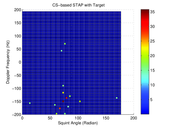
A

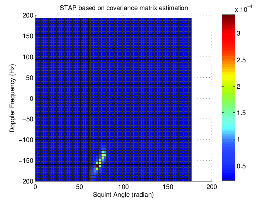
B

Figure 1: Echo amplitude of clutter and target on spatial-frequency plane

A

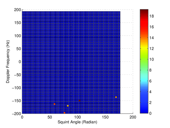
B

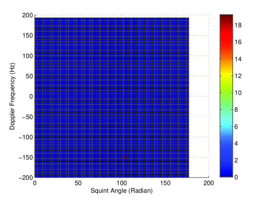
C

Figure 2: Effect of sidelobe suppressing filter

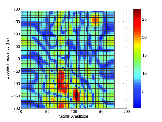
Figure 3: Effect of SMI filter

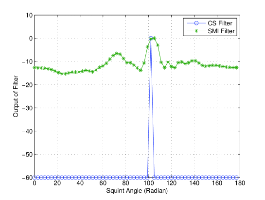
Figure 4: Output of Filter at Different Squint Angle

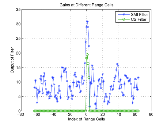
Figure 5: Output of Filter at Different Squint Angle

VI Conclusion

In this paper, a class of novel STAP algorithms based on sparse recovery technique, called CS-STAP, were given and examined. Its performance is studied by analysis of real data. The motivation for application of technique of compressed sensing on STAP is inherent sparsity of radar echo from target and clutter. Building estimator directly from sample data make CS-STAP method have ability of super-resolution and lead further to almost complete elimination of clutter. Improved performance over conventional STAP method depending on covariance matrix estimation, such as SMI, were obtained by CS-STAP method. In an application of this method to the Mountaintop data set, we showed that CS-STAP method can provide better effect of clutter suppression and more accurate estimation for Doppler frequency and azimuth angle of target than SMI detector. Furthermore, the number of training data used in CS-STAP method is much less than SMI. It means that CS-STAP method will outperform significantly SMI method when the hypothesis of stationary for clutter is violated severely.

References

- [1] R. Klemm. Principles of Space Time Adaptive Processing. Bodmin, England: IEE Press; 2002.
- [2] J.R. Guerci. Space Time Adaptive Processing for Airborne Radar. Boston: Artech House Publishers; 2003
- [3] K.R. Gerlach. Outlier resistant adaptive matched filtering. IEEE Trans. Aerospace and Electronic Systems 2002;38:885-901.
- [4] M.Rangaswamy, F.C. Lin, K.R. Gerlach. Robust adaptive signal processing methods for heterogeneous radar clutter scenarios. Signal Processing 2004;84:1653-1665.
- [5] K.R. Gerlach. Outlier resistant adaptive matched filtering. IEEE Trans. Aerospace and Electronic Systems 2002;38:885-901.
- [6] M.Rangaswamy, J.H. Michels, B. Himed. Statistical analysis of the nonhomogeneity detector for STAP applications. Digital Signal Processing 2004;14:253-267.
- [7] R.S. Adve, T.B. Hale, M.C. Wicks. Joint domain localized adaptive processing in homo geneous and non homogeneous environments. Part II: Nonhomogeneous environments. IEE Proc. Radar Sonar and Navig. 2000;147(2):66-73.
- [8] R.S. Adve, T.B. Hale, M.C. Wicks. Joint domain localized adaptive processing in homo geneous and non homogeneous environments. Part I: Homogeneous environments. IEE Proc. Radar Sonar and Navig. 2000;147(2):57-65.
- [9] D. Madurasinghe, P.E. Berry. Pre-Doppler direct data domain approach to STAP. Signal Processing 85 (2005) 1907-1920.
- [10] F. Gini, M. Rangaswamy. Knowledge Based Radar Detection, Tracking and Classification. John Wiley Sons, 2008.
- [11] W.L. Melvin, G.A. Showman, An Approach to Knowledge-Aided Covariance Estimation. IEEE Trans On Aerospace and Electronic Systems VOL. 42, NO. 3 JULY 2006. pp1021-1042
- [12] Special Section on Knowledge Based Systems for Adaptive Radar. IEEE Signal Processing Magazine 2006;23(1).
- [13] Special Section on Knowledge Aided Sensor Signal and Data Processing. IEEE Transactions on Aerospace and Electronic Systems 2006;42(3).
- [14] D. L. Donoho, Compressed Sensing, IEEE Trans. Inform. Theory. 52, n. 4, (2006), pp. 1289 C1306.
- [15] E. J. Candes, and T. Tao, Near optimal signal recovery fromrandomprojections: Universal encoding strategies? IEEE Trans. Inform. Theory, 52(12), pp. 5406 C5425, December 2006.
- [16] E. J. Candes and T. Tao. Decoding by linear programming, IEEE Trans. Inform. Theory 51, 4203 C4215, 2006.
- [17] E. Candes and M. Wakin, An introduction to compressive sampling. IEEE Signal Processing Magazine, 25(2), pp. 21 - 30, March 2008.
- [18] S. Bhattacharya, T. Blumensath, B. Mulgrew, and M. Davies, Fast encoding of synthetic aperture radar raw data using compressed sensing, IEEE Workshop on Statistical Signal Processing, Madison, Wisconsin, August 2007.
- [19] L. Potter, P. Schniter, and J. Ziniel, Sparse reconstruction for RADAR, SPIE Algorithms for Synthetic Aperture Radar Imagery XV, 2008.
- [20] K.R. Varshney, M. Cetin, J.W. Fisher, and A.S. Willsky. Sparse representation in structured dictionaries with application to synthetic aperture radar, IEEE Transactions on Signal Processing, 56(8), pp. 3548 - 3561, August 2008
- [21] W.L. Malvin, A STAP Overview, IEEE AES Magazine, Vol.19, No.1, January 2004,pp19-35.
- [22] M.R. Garey and D.S. Johnson, Computers and Intractability, A Guide to the Theory of NP-Completeness, W. H. Freeman and Company, New York, 1979
- [23] S. Boyd, and L. Vandenberghe, Convex Optimization, Cambridge University Press, 2004
- [24] J.A. Tropp. Greed is Good: Algorithmic Results for Sparse Approximation. IEEE Trans. Inform. Theory 50 (11), Oct. 2004, pp. 2231-2242
- [25] Candes, E. J., The restricted isometry property and its implications for compressed sensing, Comptes Rendus de l’Academie des Sciences, Serie I, 346 (2008), 589-592.
- [26] Juditsky and A.S. Nemirovski. On verifiable sufficient conditions for sparse signal recovery via ?1 minimization, ArXiv: 0809.2650, 2008.
- [27] G.W.Titi, An overview of the ARPA Mountaintop program. Proceedings of 1994 Adaptive Antenna Systems Symposium, Melville, NY, Nov. 1994, 53-59.
- [28] I.S.Reed, J.D.Mallett and L.E.Brennan, Rapid Convergence Rate in Adaptive Arrays, IEEE Trans on AES VOL. AES-10, NO. 6 NOVEMBER 1974
- [29] http://spib.rice.edu/spib/
- [30] www.stanford.edu/ boyd/cvx/
- [31] J. A. Tropp and A. C. Gilbert. Signal recovery from random measurements via orthogonal matching pursuit. IEEE Trans. Info. Theory, 53(12):4655 C4666, 2007.
- [32] D. Needell and R. Vershynin. Uniform uncertainty principle and signal recovery via regularized orthogonal matching pursuit. DOI: 10.1007/s10208-008-9031-3, 2007.
- [33] D. Needell and J. A. Tropp. CoSaMP: Iterative signal recovery from incomplete and inaccurate samples. ACM Technical Report 2008-01, California Institute of Technology, Pasadena, July 2008.
- [34] H.Zhang, G.Li and H.Meng, An efficient Greedy Algorithm for Sparse Recovery of Compressible Signal. Technical Report, Department of Electronic Engineering, Tsinghua University, 2009