On the Communication of Scientific Results: The Full-Metadata Format

Abstract

In this paper, we introduce a scientific format for text-based data files, which facilitates storing and communicating tabular data sets. The so-called Full-Metadata Format builds on the widely used INI-standard and is based on four principles: readable self-documentation, flexible structure, fail-safe compatibility, and searchability. As a consequence, all metadata required to interpret the tabular data are stored in the same file, allowing for the automated generation of publication-ready tables and graphs and the semantic searchability of data file collections. The Full-Metadata Format is introduced on the basis of three comprehensive examples. The complete format and syntax is given in the appendix.

1 Introduction

In the last few years an increasingly sophisticated experimental infrastructure has evolved enabling scientists to share not only knowledge but also primary data via scientific publications [1, 2, 3]. With this increase in sharing primary or processed scientific data the lack of intuitive and well defined data formats for simple tabular data has become increasingly obvious. For complex data sets like the ones dealt with in the earth sciences, adequate binary formats like the Network Common Data Form (netCDF [4]) or the Hierarchical Data Format (HDF [5]) are well established [6, 7], and the publication of observational geophysical data in World Data Centres has developed into an effective mechanism for the exchange of data [8]. Another example is the information technology infrastructure for handling the data of the ATLAS experiment [9], where the event data is mainly stored in the ROOT file format [10]. For less complex data structures, like tabular data as typically encountered in many parts of natural and technical sciences, no single standard format has evolved.

The success of the HDF and netCDF relies on the fact that the formats are well defined and integrate smoothly into the workflow of scientists in different laboratories. Although these formats are capable of storing and documenting simple tabular data, the overhead of work needed to process binary files generally poses a barrier to the use of these formats in fields where complex data structures are seldom dealt with.

A natural requirement of a standardized file format for tabular data is that it allows scientists to add observations, notes, parameter specifications and analysis results by editing in clear text using any given text editor. This constitutes what most of the overwhelming number of data formats used in laboratories around the world have in common. However, as text files are easy to handle, every laboratory, working group or even scientist has an individual standard of documenting scientific results with text-based formats. While this is completely sufficient in a short term perspective, it becomes intractable with the tendency of research projects to rely on the cooperation of international consortiums involving many different laboratories. Furthermore, in publishing scientific results, there is an increasing demand to provide also processed data as supplementary data or to even publish primary data in OpenData repositories [2]. Thus, there is a need for a common data format for tabular data which is:

Readable and self-documenting:

The data should be written in the same way the scientist is used to reading it, as e.g. in a laboratory notebook. It should be clear, text based and processable with any word processing tool. The file format should include sections which allow the scientist to document the data and its origin, and this to such an extent that no other source be required to to understand the origin of the data. This standard also implies that the data files are search-able and individual data sets can be tracked down by semantic or keyword based queries.

Flexible but structured:

The data format must be flexible enough to allow the individual scientist to structure and classify data in an intuitive and convenient way without compromising the overall structure and readability as stipulated by the format. The overall structure of the format must be such that data files may still be processed with common analysis and visualisation software packages, thus facilitating the automated processing of data from different measurement sources and measurement series. This further implies that format and syntax specifications are largely decoupled such that annotated data may smoothly cross language zones.

Fail-safe and compatible:

A fail-safe data format has to assure that the format is robust against misinterpretation by a parser or deviations from the format specifications. As the format specification is expected to evolve in time, backwards compatibility must always be retained.

Searchable:

Communicating scientific results implies that relevant data sets can be found within a certain collection by means of simple queries. This requires the documentation of scientific data in the form of self-documenting file formats. Further, a collection of scientific data files must be catalogued not only according to bibliographic items or keywords, but also to physical quantities.

It is of paramount importance that the data format integrates smoothly into the existing workflow of the scientist and supports the natural working cycle of collecting and structuring information. To become widely accepted, the threshold of annotating primary data with additional information must be as low as possible; scientists should not have to start learning a complex syntax or a sophisticated mark-up language, which for all practical purposes will require specialised software tools.

In the following we present a syntax for a self-documented scientific data file format for tabular data sets which we call the Full-Metadata Format (FMF). It is purely text based and FMF-files consist of two parts: the first part contains the metadata describing the data written in the second part of the file. Because most scientific software tools support the skipping of some initial header lines, the data stored in the FMF-file can directly be processed as usual. Yet, the documentation of the data remains always at hand. The proposed file format has evolved from the development of high-throughput experimental setups for the processing and characterisation of organic solar cells [11, 12, 13], and is applicable to all kinds of tabular data encountered in the natural sciences and engineering. A further demonstration of the capabilities of the FMF-format is constituted by its incorporation into the scientific analysis software Pyphant [14, 15], which supports the computation with units and the analysis of metadata [16, 17].

Below the Full-Metadata Format is first described by means of two examples highlighting its principles and potential. A third example sketches the capabilities of searching the metadata of FMF-files for relevant data sets. In the appendix the complete format and syntax definitions are listed.

2 A Basic Example: Communicating Simple Tabular Data

In this example a typical data exchange between two work groups is considered to demonstrate the benefit of human readable data formats for the communication between scientists. The goal of the cooperation might be the enhancement of the power conversion efficiency of organic solar cells, or the numerical modelling of the characteristics of solar cells with respect to production parameters. This requires exchanging data between the groups. In Fig. 1a the screenshot of a typical data set of a current-voltage characteristic is shown, which is formatted in the most common data format for tabular data: pure columns of numbers. The corresponding graphics is shown in Fig. 1b. The missing axis labels indicate that important information like the name, symbol, and units of the plotted physical quantities are not provided with the data set, thus only allowing for a qualitative assessment of the data.

(a)	(b)

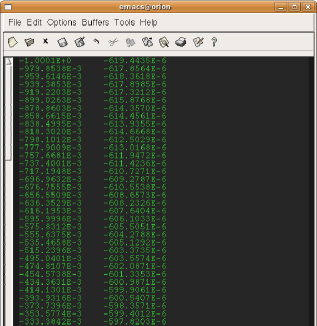
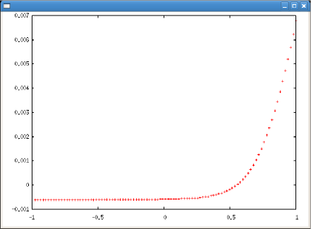
Figure 1: A typical data file exchanged between scientists. (a) Screenshot of a text editor’s view of the data file and (b) the corresponding plot with a qualitative relation from the values listed in the data file.

This lack of information can be clarified by a phone call or an email. Typically, the response to such requests depends on how the working group internally documents the primary data. It may either be well documented by means of protocols in the laboratory notebook of the scientist in charge, but the protocol has not been attached to the e-mail, or the data file format is standardised by an internal format convention of the working group, but the format has not been documented. In both cases a useful response would at least communicate that the first column is voltage $V$ in units of Volt, the second column is current $I$ in units of Ampere, the current $I$ is measured as a function of $V$, the device has an active area $A_{pv}$ of 5.3mm², and is exposed to an illumination intensity $I_{AM1.5}$ of 100mW/cm² [18]. Having this information at hand, the diagram can be labelled correctly as required for further processing, publication, and understanding (Fig. 2). In addition, characteristic properties like the fill factor ($FF=45.5\%$) and the power conversion efficiency ($\eta=2.95\%$) can be extracted from the data [18]. However, this is only a temporary solution, as the original data file is unlikely to be annotated accordingly. The next time the data set is used, the same questions will arise. The data set might even become completely useless, if the relevant protocol of the laboratory notebook cannot be identified anymore or if the person responsible for the measurement cannot clarify the units [19].

Figure 2: Publication-ready graphics of an IV-characteristic based on a Full-Metadata Format file (Fig. 3): IV measurement for substrate S419, pixel 9. The solar cell characteristics are measured under illumination with a mismatch corrected intensity of $I_{AM1.5}=100\mathrm{mW/cm}^{2}$.

Clearly, it would have been better to annotate the data set with the missing information right from the start. Using the proposed format, the FMF-file corresponding to the data depicted in Fig. 2 is shown in Fig. 3. Some metadata and the first few lines of the raw data are shown. The list of metadata is not exhaustive and only as much is shown as to highlight the possibilities of the file format. Note, that the proposed file format has similarities with the INI file format, but goes beyond this in its possibilities due to extra rules. The detailed syntax is given in A.

\psfrag{qq}{$\vdots$}\includegraphics[width=267.97551pt]{Fig3}

Figure 3: The first lines of a self-documented data file in the Full-Metadata Format [20], cut after some tabular data values.

The file shown in Fig. 3 starts with a single line describing the version of the Full-Metadata Format. The next part contains all the metadata required for understanding the actual data. This metadata is given in a simple and user-friendly way by structuring the file into sections. Bibliographic information resides in section [*reference], column definitions in section [*data definitions], and the corresponding columns of data in section [*data]. The bibliographic information is either used for internal archiving purposes or for publishing the data file in an OpenData repository [2] like for example [20]. These three sections are mandatory and comprise the fundamental structure of a Full-Metadata Format-file.

The other sections in the example in Fig. 3, [setup], [parameters], and [fingerprints] are not preceded by an asterisk. These are user defined sections and can contain arbitrary extra metadata. All sections, except the [*data] section, contain items coded as colon separated

$$key:value$$ (1)

pairs. The $key$ cannot be a colon, because the first colon per line separates $key$ and $value$. A $value$ can be boolean, numerical, a quantity, a timestamp, or a string. In [*data definitions] section the value must be a column specificator (A.3).

According to the meta data, the file shown in Fig. 3 was created by Moritz Riede on 17th of April 2006 at 18:55:38 local time, which is 2 hours ahead of UTC (cf. Tab. 6). It contains data for the solar cell on pixel 9, located on a substrate with the unique identifier S419. This identifier can be used for referencing the processing and measurement history of the solar cell [12, 19]. A short comment completes the [*reference] section.

The section [setup] is used in the example to describe the measurement type and the setup used. Many measurements can be carried out on different setups, each with their own distinct features, which are relevant when interpreting the data [12, 13]. A set of important measurement parameters important to the interpretation of the data are recorded within the section [parameters]. A special mention should be given to key-value pairs which we characterize as quantities, and in section [parameters] for example, the active area of the solar cell is specified as:

pixel area: A_{pv} = 5.3 mm^2

It is written like a typical parameter specification and comprises a name (“pixel area”), a symbol in LaTeX-notation ($A_{pv}$) [21], and a numerical value and a unit (which might be omitted for unit-less values). LaTeX-notation symbols other than characters of the Latin alphabet can easily be included. Quantities also support the specification of measurement uncertainties and estimation errors (cf. Tab. 5). The last item shown in section [parameters] is boolean, indicating that the measurement was carried out in 4-wire mode.

First analysis results derived from the raw data of solar cell pixel 9 on substrate S419 are listed in the section [fingerprints]. As such data is redundant, but can be very helpful for a quick overview and processing of the recorded data.

The last two sections, [*data definitions] and [*data] differ from the preceeding sections before: the $n^{\rm{th}}$ line of [*data definitions] describes the $n^{\rm{th}}$ column of the following [*data] section containing tabular measurement data. The format of the column description is chosen to resemble a typical axis label having a name, a symbol, and a unit in brackets. In addition, the functional relation of the tabulated quantities is given by explicitly denoting current $I(V)$ being measured in dependency on voltage $V$.

3 A More Complex Example: Documenting Experiment and Analysis Together

Applying the basic example of Sec. 2 to other data sets quickly reveals, that for general purposes a more capable syntax is often needed. For example measurement errors have to be specified or more than one table may be needed for a comprehensive description of the data sets.

An example of an FMF-file with two tables is shown in Fig. 4. It documents the work of two students in measuring Faraday’s constant in the course of a practical exercise [22]. The experiment relies on Faraday’s second law and uses a Coulometer for measuring the volume fractions of hydrogen and oxygen evolving due to a constant current $I$ being applied to an aqueous solution of sodium hydroxide. From these time series Faraday’s constant can be computed by converting the volume fractions to normal conditions (1023mbar and 273K), estimating the evolved volume per time interval $V^{\prime}$ from the time series, and evaluating

$$\mathrm{Fa}=22.4\frac{\ell}{\mathrm{mol}}\cdot\frac{I}{N_{e}V^{\prime}}$$ (2)

both for hydrogen and oxygen. Therefore, room temperature and barometric pressure at the time of the experiment comprise important metadata for evaluating the measurement. These physical quantities are specified in section [measurement] of the FMF-file shown in Fig. 4 together with their measurement uncertainties:

room temperature: T = (292 \pm 1) K
barometric pressure: p = 1.0144 bar \pm 10 mbar

This section also notes the current $I$, which is applied to the sodium hydroxide solution, and its measurement error. Note that the error specification is very similar to the way in which a scientist would describe the data in a report. Other possibilities for specifying errors are listed in Tab. 5 of the Appendix.

\psfrag{ldo}{$\ldots$}\includegraphics[width=346.89731pt,bb=95 73 567 755]{Fig4}

Figure 4: Measurement of Faraday’s constant - An example of documenting experimental data and their analysis within one FMF-file [22].

Because the experiment deals with two different gases, namely hydrogen and oxygen, which differ in terms of their number of electrons $N_{e}$ per reaction, Faraday’s constant is individually retrieved for each time series. Therefore, two tables are needed for adequately describing the experiment: one table specifying the material parameters and the result of the data analysis and another table listing the time series of measured volume fractions. The names of these tables as well as the associated symbols are defined in section [*table definitions] of the FMF-file in Fig. 4. It tells that the table named analysis, $A$, is followed by the table primary, $P$. Each table then consists of sections [*data definitions:]$X$] and [*data:]$X$] with $X$ referencing the symbol of the table such that each pair can easily be identified.

In this example, two cases of error specifications are needed in the tables: namely specifying constant measurement errors valid for elements of a specific column, and assigning special error columns. The specification of constant measurement errors is shown in section [*data definitions: P] of the second table in Fig. 4:

time: t [min] \pm 5 [s]
hydrogen volume: V_{H_2}(t) \pm 0.2 [cm^3]
oxygen volume: V_{O_2}(t) \pm 0.2 [cm^3]

In the example, time $t$ is measured in units of minutes with an accuracy of 5 seconds and volumes $V_{H_{2}}(t)$ and $V_{O_{2}}(t)$ are measured in units of cm³ with an accuracy of $0.2\mathrm{cm}^{3}$. With this information at hand, the primary data of section [*data: P] can be plotted as shown in Fig. 5.

Figure 5: Measurement of Faraday’s constant. The diagram visualises the table of data documented in section [*data: P] of Fig. 4 and uses information from section [*data definitions: P] to label the graph accordingly [22].

The specifications of non-constant errors are shown for $V^{\prime}$ and Fa in Fig. 4. The errors $\Delta_{V^{\prime}}$ and $\Delta_{Fa}$, respectively, are defined in section [*data definitions: A] and are explicitly related to the measured quantity as:

Faraday constant: Fa \pm \Delta_{Fa} [C/mol]
error of Faraday constant: \Delta_{Fa} [C/mol]

These data definitions mean that the column listing the Faraday-constant is followed by a column with the corresponding measurement error. Because this table consists of six columns, the creator of the FMF-file decided that the readability would be improved by starting section [*data: A] with a comment repeating the symbols defined in section [*data definitions: A]. The comment is introduced by a leading semicolon.

Alltogether, sections [*data definitions: A] and [*data: A] of Fig. 4 give a simple textual representation of Tab. 1, which could be the summary of an experiment. Section [*data definitions: A] lists the name of the gas, the number $N_{e}$ of electrons per reaction, the ratio $V^{\prime}$ of released gas per time interval and the resulting Faraday constant. The estimated values of Faraday’s constant depend on the number $N_{e}$ of electrons per reaction. As can be seen from the last column of Table A in Fig. 4 the measurement of Faraday’s constant deviates up to 6% from the precise value of Fa=96485.3399(24) C/mol [23], but has been correctly determined within the error margins.

In this case the constant has been determined by means of the line of best fit. Years later it occures to the students (or maybe even their successors in the practical exercise) that moving a ruler around on a piece of paper is perhaps not the best way to analyse the data. Since the primary data is available in a form easily understood, they decide to redo the analysis with the more sophisticated means of a least square fit while taking into account, that the anode is likely to have an oxide layer, which increases $V^{\prime}_{O_{2}}$ in the beginning of the experiment. With $V^{\prime}_{H_{2}}=1.202\mathrm{cm}^{3}/\mathrm{min}\pm 1.0\%$ and $V^{\prime}_{O_{2}}=0.596\mathrm{cm}^{3}/\mathrm{min}\pm 2.2\%$ Faraday’s constant is now determined as $95600\pm 1500$ C/mol for H₂ and $96500\pm 2700$ C/mol for O₂. Both these values are far more accurate compared to the original results. This improvement was possible, because the original information was preserved in a way that allowed its interpretation. Furthermore it could be understood, because the method of analysis was indicated.

While this example might seem a trivial, it is common that data experimentally gathered by one scientist would be useful to another one years later. Often the first scientist has become unavailable and the data can no more be found, let alone understood. This is a waste of resources that should be reduced.

gas	$N_{e}$	$V^{\prime}\pm\Delta_{V^{\prime}}$ [cm3/min]	$\mathrm{Fa}\pm\Delta_{Fa}$ [C/mol]
H2	2	$1.256\pm 0.065$	$91400\pm 5500$
O2	4	$0.562\pm 0.04$	$102200\pm 7800$

Table 1: Formatted analysis table $A$ of the FMF file shown in Fig. 4. The table lists the name of the gas, the number $N_{e}$ of electrons per reaction, the ratio $V^{\prime}$ of released gas per time interval and the resulting Faraday constant. The ratio $V^{\prime}$ has been determined from table $P$ (Fig. 4) by plotting volume fraction against time for each gas (Fig. 5) and estimating the line of best fit.

4 An advanced example: Searching Scientific Data in terms of units

How to search for certain physical quantities is explained on the basis of an example given in Tab. 2, where we consider the four energy related quantities pertaining to different experiments; namely work $W=23\mathrm{kJ}$, energy $E=10\mathrm{keV}$, calorific value $H=10\mathrm{kcal}$, and power $P=0.01\mathrm{MW}$. A classical full-text search cannot reveal any correlation between their notation work, energy, calorific value, and energy. The same holds for the units kJ, keV, kcal, and MW. Therefore, a question like

“Which measurements determine in an energy range between one thousand and one billion Joule?”

cannot be formulated as a full-text query. Instead, the elements of $\mathbb{M}=\{W,E,H,P\}$ have to be identified which are energies and also lie in the desired interval $[1\mathrm{kJ},1\mathrm{MJ}]$:

$$\mathbb{M}_{E}=\{m\in\mathbb{M}|\mathrm{dim}\;m=L^{2}TM^{-2}\}\cap[1\mathrm{kJ},1\mathrm{MJ}].$$ (3)

Here $L$, $T$, $M$ represent the dimensions length, time and mass, respectively.

The computation of this intersection can be carried out by normalising the elements of $\mathbb{M}$ to basic SI-units and decomposing each quantity into an 8-tuple, the elements of which are its measure and the powers of its dimensions. In terms of pattern recognition, this 8-tuple is denoted feature vector. E.g. a physical quantity $q$ is uniquely characterised by its feature vector $\vec{q}_{F}=(q_{0},\ldots,q_{7})$ with

$$q=q_{0}\cdot\mathrm{m}^{q_{1}}\cdot\mathrm{kg}^{q_{2}}\cdot\mathrm{s}^{q_{3}}\cdot\mathrm{A}^{q_{4}}\cdot\mathrm{K}^{q_{5}}\cdot\mathrm{mol}^{q_{6}}\cdot\mathrm{cd}^{q_{7}}.$$ (4)

Here $q_{0}=\{q\}$ is the measure of $q$ and $q_{1},\ldots,q_{7}$ define its unit:

$$[q]=\mathrm{m}^{q_{1}}\cdot\mathrm{kg}^{q_{2}}\cdot\mathrm{s}^{q_{3}}\cdot\mathrm{A}^{q_{4}}\cdot\mathrm{K}^{q_{5}}\cdot\mathrm{mol}^{q_{6}}\cdot\mathrm{cd}^{q_{7}}.$$ (5)

As regards the example in Tab. 2, all powers except length, time and mass are zero and only quantities given in units of $\mathrm{m}^{2}\mathrm{kg}\,\mathrm{s}^{-2}$ $(q_{1},\ldots,q_{7})=(2,1,-2,0,0,0,0)$ are energies and therefore are relevant for determining $10^{3}\leq q_{0}\leq 10^{6}$. Consequently, from the quantities listed in Tab. 2 only the quantities work $W=23\mathrm{kJ}$ and calorific value $H=10\mathrm{kcal}$ pertain to experiments determining energies between 1kJ to 1MJ.

This example illustrates how scientific data sets can be made searchable on the basis of an adequate documentation, such that the documentation of data sets directly enables the re-usability of scientific results.

	feature vector $\vec{q}$ (4)
meta-information	$q_{0}$	$q_{1}$	$q_{2}$	$q_{3}$	$q_{4}$	$q_{5}$	$q_{6}$	$q_{7}$
work: $W$ = 23 kJ	$23\cdot 10^{3}$	2	1	-2	0	0	0	0
energy: $E$ = 10 keV	$1,602\cdot 10^{-15}$	2	1	-2	0	0	0	0
calorific value: $H$ = 10 kcal	$41,9\cdot 10^{3}$	2	1	-2	0	0	0	0
power: $P$ = 0.01 MW	$10\cdot 10^{3}$	2	1	-3	0	0	0	0
search interval	$[10^{3},10^{6}]$	2	1	-2	0	0	0	0

Table 2: Classification of physical quantities by means of feature vectors. The feature vector $\vec{q}$ (4) of quantity $q$ is an 8-tuple, which is composed from the measurand $q_{0}=\{q\}$ in basic SI units and its dimension coded as powers of units (5). Feature vectors with identical elements $q_{1},\ldots q_{7}$ correspond to the same physical quantity.

5 Discussion

We have shown how a text file can used as scientific data format enabling storage of tabular data sets in a consistent and self-descriptive fashion. The real novelty of the presented data format is its systematic way in which all relevant metadata needed to understand the data can seemlessly be included. In language of the data-information-knowledge-wisdom hierarchy [24] this means that the data set is upgraded from the data level to the information level. The promotion to the information level has significant advantages:

First, it improves the capability of scientists to communicate scientific data. This may occur within a working group, with external cooperators, or within the scientific community in general. Because unhindered communication is one of the most important preconditions for a successful collaboration, this aspect cannot be overestimated. Second, it facilitates the long-term integrety of scientific data; e.g if primary data from old project must be revisited many years after or if data is passed on to comimg generations of scienctists. At present, it is rather the rule than the exception that the scientist is not able to find all relevant metadata to understand an old data set. Often such data-erosion is simply due to the meta data residing on a different data storage medium than the primary data itself. Working with a data format which embodies the relevant metadata avoids this problem altogether.

Using a self-describing format like the one presented here therefore increases the longevity of primary data and thus may improve the quality of science in general. Especially in scientific communities like the geo-sciences or high-energy physics this has proven to be the case. In these fields, large data sets and the pressure to communicate them effectively has led to a standardisation of data formats and a culture of sharing such data. Due to the complexity of the data generated in those fields more sophisticated file formats such as HDF5, netCDF or ROOTS [5, 4, 10] are in use.

In contrast to these complex data formats, the Full-Metadata Format is designed with the needs of so-called Small Science [25] in mind. Research by small working groups and individuals producing simple tabular data still occupies a central position in most scientific disciplines. Although the awareness of a systematic management and sharing of data is already rising, an appropriate data format for Small Science has yet to fully evolve. One obstacle is that data documentation using the existing extensible markup languages (XML) like XDF [26] or VOTables [27] simply add too much overhead to the content, and are cumbersome to read, edit, and process with existing scientific software tools.

The approach presented in this paper is simple: Describing simple tabular sets of data with simple text files in a way which is natural for scientists and engineers requires a minimum of change in the individual workflow and habits. In general this means documenting the metadata in a way one would like to read it in a laboratory journal or in a paper, e.g. within a diagram or a figure caption. The use of plain text files ensures that the scientist can apply this documentation technique instantaneously with basic information technology infrastructure. Still, these text files can be parsed in a very easy way due to their simple structure [15].

Because of its simplicity and the self-describing character the Full-Metadata Format offers many possibilities:

• The clear-text documentation of scientific data simplifies its re-usage.

• The usage of plain text files makes the data ideal for long term preservation [28].

• The communication of the data does not need a complex infrastructure; text files can be sent by email or even be printed to analogue media.

• Because the data is connected to the relevant units, special software which is able to process these units during scientific data analysis like Pyphant [14, 15] can be used sucht that processing and visualisation of the data can be automated.

• Furthermore, the use of the relevant units enables a semantic search within a collection of data sets.

A drawback of the Full-Metadata Format results from the fact, that the end-of-line (EOL) character of text files is not uniquely defined for all operation systems, which causes text files to be displayed incorrectly after being transfered to a different type of operation system. However, this problem is generally known and appropriate tools are available [29].

6 Conclusion

The advantage of the suggested file format is its ease of use and its scientist-friendly syntax, which is in contrast to the computer-friendly syntax of markup-languages. The purpose of the Full-Metadata Format is to document small tabular data sets, mainly produced in fields generalised as Small Science. For these scientific communities, the use of the Full-Metadata Format can be the starting point to a systematic management of scientific data in the form of information, and thus the starting point for participation in the growing culture of data sharing.

The authors would like to encourage the reader to engange in the application of the Full-Metadata Format and to actively participate in the improvement of the proposed format.

Appendix A The Syntax of the Full-Metadata Format

The appendix comprises a more technical description of the syntax characterising the Full-Metadata Format. It is meant as a guide to the format and shows comprehensive tables of coding examples. Therefore the appendix intentionally repeats certain parts of the format in order to minimise browsing for a specific piece of information.

Data files written in the Full-Metadata Format always consist of three parts:

Headline

(A.1),

Metadata

(A.2),

Tables

(A.3).

The headline is a comment indicating how to interpret the file on a formal level. Following the headline is the main body of the file, which is structured in sections. While the file body can contain arbitrarily many sections with metadata and measurement data, at least three mandatory sections are needed for a meaningful FMF-file. These sections are named [*reference], [*data definitions] and [*data]. The [*reference] section contains the metadata necessary for referencing the data set and the [*data definitions] and [*data] sections represent a table of data. This minimal structure is shown in Fig. 6, while the general structure is summarized in Fig. 7.

Figure 6: Minimal structure of a Full-Metadata Format-file.

Figure 7: The general structure of an FMF-file. The headline is used to define the file coding and delimiter in the tables, of which several are present in the file.

¿From a grammatical point of view, the Full-Metadata Format consists only of three different types of lines, defined as follows:

Comments

are indicated by a leading semicolon (;) or a leading sharp (#). The comment character used for the headline (A.1) has to be used consistently for all other comments in the same file. A comment character in a key or value is treated as a normal character.

Section headers

are embraced by square brackets $[\;]$ and have to be unique throughout the file. Section names starting with an * are reserved for use in this specification or any future version thereof. Any other legal character sequence can be used for arbitrary sections. In this version, the following reserved sections are put to use:

• [*reference],

• [*table definitions],

• [*data definitions], and

• [*data].

Key:value items

are used in all but the [*data] section. A key can consist of all characters except the colon (:), which is used to separate key and value. Each key has to be unique within its section. The different types of values are discussed in A.2. In the [*reference] and all user defined sections, arbitrary value types may be used. The [*table definitions] section may only contain symbols as values and the [*data definitions] sections only column specifications, both for reasons that will become clear later on.

Rows of data

are collected in [*data] sections. They represent classical tabulated data sets. Other column separators than tab stop can be specified in the headline (A.1).

A.1 Headline

The headline is a special comment, which indicates how the content of the file is to be interpreted. This includes foremost the encoding, which tells the computer how to translate the bytes of the file into characters and the separator, which splits the table rows of the [*data] section into the appropriate cells. It also mandatorily specifies the version of the Full-Metadata Format employed in the file. It uses the Emacs style file syntax [30] and thus looks like

⬇

; -*- fmf-version: 1.0 -*-

In addition, coding (default = utf-8) and delimiter (default=tab) can be specified (Tab. 3). The key:value items have to be separated by a semicolon. Although the semicolon (;) is the default comment character, comments can alternatively be introduced by a hash (#). The comment character used in the headline has to be used throughout the file.

A.2 Metadata

Metadata is an essential part of the data file, because it describes the context from which a data set has been collected. It is structured by sections, which start with a unique section header consisting of a section identifier enclosed in square brackets. Section identifiers starting with an asterisk are reserved for this or any future version of this specification. All section headers except the [*data]-header are followed by lines of

⬇

key: value

The key can contain any valid character except a colon, which separates key and value. The value is always a textual representation of some information. However, in order to allow for an automated interpretation of the information the Full-Metadata Format defines some conventions for the representation of numerical and boolean values, quantities and complex strings:

Boolean values

are given by the words “true” or “false”. They can be written in lower case letters, capital letters, or with a starting capital letter. A list of boolean values is defined by separating the individual values by commas.

Numerical values

are textual representations of integer, real or complex scalars. Due to the restrictions of floating point arithmetics, the accuracy of real and complex scalars is restricted by the number of bits used for encoding the scalar. Optionally, a numerical value can be complemented by an uncertainty specified in common scientific notation. Furthermore a numerical value can be annotated by a symbol in LaTeX-notation, which is prefixed to the number and is related to the latter by an equal sign. A list of numerical values is defined by separating the individual values by commas. A comprehensive list of possible numerical formats is given in Tab. 4.

Quantities

are measurands, estimations, or control parameters of an experiment or simulation. They are characterised by a numerical value and a unit. Units are extensively described in B. A list of quantities is defined by separating the individual quantities by commas. A comprehensive list of examples of quantities is given in Tab. 5.

Timestamps

are ISO formatted date-time strings [31], for example ”2006-04-17 18:55:38+02:00” for 17th of April 2006 with 18:55:38 local time, which is 2 hours ahead of UTC (Tab. 6). If the time zone information is omitted, the local time zone is assumed. However, in view of international cooperations the reference to UTC should always be included. A timestamp can also be admended by an uncertainty, which is indicated by +- and a temporal quantity. This is useful for applications of legal medicine [32]. A list of timestamps is defined by separating the individual timestamps by commas.

Strings

are the most flexible type of values to be returned, because a string of characters can map any textual information. In particular this applies if the mapping to boolean values, numerical values, quantities, or timestamps does not match. In order to prevent the interpretation of a textual value in terms of numerical values or quantities the information can always be enclosed in quotation marks. However, for more complex strings like multi-line strings, lists of strings or strings containing quotation marks, some conventions have to be met, which are listed in Tab. 7.

A.3 Tables

The [*tables] section is a means to include more than one table in a single FMF-file. This creates the need to identify corresponding [*data definitions] and [*data] sections. To this end, each table is assigned a name and a symbol, which in turn is used for identifying the table throughout the file. This information is found in the [*tables] section. The relevant sections for multi-table files are:

[*table definitions]

This section has one key:symbol item per table. While the key acts as a descriptive name for the table, the symbol is used to relate the [*data definitions] and the [*data] sections to each other. Therefore these sections reference the table $symbol$ within their section header as [*data definitions: symbol] and [*data: symbol]. The [*table definitions] section can be skipped, if only one table is given within the FMF-file. In this case, the data definitions and the data sections do not reference a symbol and thus are captioned by [*data definitions] and [*data] (see Fig. 6). In general, LaTeX-notation for symbols is allowed.

[*data definitions]

These sections describe the columns of data given in the respective [*data] sections by means of key:column items. The $n^{\mathrm{th}}$ item of a [*data definitions] section describes the $n^{\mathrm{th}}$ column in the [*data] section. A column value specifies a symbol referencing the tabulated quantity. Optionally, it can also define the functional dependency on another quantity, a unit and an uncertainty, which is either constant or might be tabulated in another column. For the details refer to Fig. 8.

Figure 8: Structure of the tables part comprising two tables.

[*data]

These sections are tables of data as shown in Figs. 3 and 4. The columns can contain strings, numerical values, and quantities, whose symbols and names are defined in section [*data definitions]. The same holds for uncertainties and units. By default, columns are separated with tabs. Other delimiter like whitespace can be explicitly defined in the header line of the FMF-file (Table 3).

Variable   :	Value	Status
fmf-version   :	1.0	Mandatory. Version presented in this paper is 1.0.
coding   :	utf-8	Default character encoding [33].
:	cp1252	Example for character encoding with WinLatin1 code page [34].
delimiter   :	\t	Default delimiter is tab.
:	whitespace	Example for column separation by whitespaces.
:	semicolon	Example for column separation by semicolons (;).
:	,	Example for column separation by commas.

Table 3: Variables defined in the headline. Comprehensive information on alternative code pages can be found at [35].

Explaining key   :	Value
Integer   :	1
Negative integer   :	-2
Floating point number   :	1.0
Floating point number with leading decimal dot   :	.1
Floating point number with exponential   :	1e-10
Another floating point number with exponential   :	-1.1E10
Complex number   :	1+2j
Another complex number   :	1.1+2J
Complex number with zero real part   :	2J
Complex number with zero imaginary part   :	1+0J
List of floats   :	1.0, .1, 1e-10, -1.1E10
Parameter   :	P = 42.0
Parameter with uncertainty   :	Q = 42.1 +- 0.2
Parameter with relative uncertainty   :	Q’ = 42.1 +- 0.48%

Table 4: Examples for textual representations of scalars. A value is interpreted as integer if the respective string contains only digits and an optional leading sign. A string is interpreted as floating point number if it contains a decimal dot or an exponent indicated by an embedded ’e’ or ’E’. Complex numbers are coded as a sum of real and imaginary parts in integer or floating point notation. The imaginary part is indicated by a trailing ’j’ or ’J’. Lists of numbers are built from comma separated numbers. Special values like NaN (not a number) or +INF and -INF for $\pm\infty$ are also allowed (IEEE 754) [36]. Optionally numerical values can be complemented by uncertainties and a symbol in LaTeX-notation. Note that the uncertainty sign can also be given by $\backslash$pm.

Explaining key   :	Quantity
Physical quantity   :	2.0 ohm
:	2.0 kg*m**2/A**2/s**3
:	2.0 kg*m$\hat{\;}$2/A$\hat{\;}$2/s$\hat{\;}$3
:	2.0 kg*m$\hat{\;}$2*A$\hat{\;}$-2*s$\hat{\;}$-3
Physical quantity with uncertainty   :	2.0 ohm +- 0.02 ohm
:	2.0 ohm +- 20 mohm
:	(2.0 +- 0.02) ohm
:	(2.0 +- 1 %) ohm
:	(1.0 +- 0.01) 2.0 ohm
:	(1.0 +- 1%) 2.0 ohm
Monetary quantity   :	19.99 EUR/m**2
List of quantities   :	2.0 ohm, 2.0 ohm +- 0.02 ohm, 19.99 EUR/m**2
Resistance   :	R = 2.0 ohm
Temperature   :	$\backslash$theta = 32.0 K
Measured resistance   :	R = 2.0 ohm +- 0.02 ohm

Table 5: Examples for textual representations of quantities. They are specified by a numerical value (Tab. 4) and a unit (B). Optionally, quantities can be complemented by uncertainties and a symbol in LaTeX-notation. Note that the uncertainty sign can also be given by $\backslash$pm.

Explaining key   :	Value
date   :	2008-12-16
week date   :	2008-W47-1
date-time   :	2008-12-16T16:51
another date-time   :	2008-12-16 16:51
date-time with seconds   :	2008-12-16T16:51:05
date-time UTC   :	2008-12-16T16:51Z
date-time+2h   :	2006-04-23 14:25:51+02:00
date-time with uncertainty   :	2008-12-16 16:30+-2 h
list of dates   :	2008-11-17,2008-1-3,2006-·2-17,2008-W47-1

Table 6: Examples for ISO formatted date-time strings [31].

Explaining key   :	Value
Text   :	Demonstrating the flexibility of the Full-Metadata Format
Comma separated list   :	Freiburger Materialforschungszentrum, University of Freiburg
Quoted text   :	”Freiburger Materialforschungszentrum, University of Freiburg”
Single quote   :	’Freiburger Materialforschungszentrum, University of Freiburg’
Inside quotation   :	Arthur C. Clarke’s ”The Sentinel”
Multi-line   :	”’A multi-line value, that spans more than one line:
The line breaks are included in the value.”’
Another multi-line   :	”””A multi-line value, that spans more than one line:
line breaks are included in the value.”””
Enclosed quotation marks   :	””” ”Don’t visualise data, document it!” ”””

Table 7: Examples for textual representations of information, which are mapped to strings of characters. Text values can be quoted by single quote, a single forward apostrophe (’) and by double quotation marks (”) in order to prevent the interpretation of the text value by the parser. Triple quotes are used for multi-line text values or in cases for which the text value starts and ends with quotation marks.

Appendix B Units

Units are defined on the basis of the SI units Metre (m), Kilogram (kg), Second (s), Ampere (A), Kelvin (K), Mol (mol), Candela (cd), and the derived units Newton (N), Pascal (Pa), Joule (J), Watt (W), Coulomb (C), Volt (V), Farad (F), Ohm (ohm), Siemens (S), Weber (Wb), Tesla (T), Henry (H), Lumen (lm), Lux (lx), Becquerel (Bq), Gray (Gy), Sievert (Sv), Radiant (rad), and Steradiant (Sr). Moreover, monetary values can be defined on the basis of the Euro (EUR) exchange rates as published by the European Central Bank [37]. The order of magnitude for all units can be specified by metric prefixes (Tab. 8). Constants and additional non-SI units are listed as follows:

Tab. 9

Mathematical and physical constants.

Tab. 10

Time units.

Tab. 11

Length and area units.

Tab. 12

Volume units.

Tab. 13

Mass and force units.

Tab. 14

Energy and power units.

Tab. 15

Pressure units.

Tab. 16

Geometrical and thermo-dynamical degrees.

Note that the abbreviation “a.u.” is used for arbitrary units and not for atomic units. This is due to the fact, that atomic units form a system of units in which several physical constants are defined as unity [38]. E.g. for Hartree atomic units the mass and charge of the electron, the Bohr radius, the absolute value of the electric potential energy of the Hydrogen atom in its ground state, Planck’s constant and the permittivity of vacuum are unity by definition, which of course collides with the searchability of scientific data discussed in Sec. 4.

Symbol	Prefix	Order of magnitude
Y	yotta-	$10^{24}$
Z	zetta-	$10^{21}$
E	exa-	$10^{18}$
P	peta-	$10^{15}$
T	tera-	$10^{12}$
G	giga-	$10^{9}$
M	mega-	$10^{6}$
k	kilo-	$10^{3}$
da	hecto-	$10^{2}$
d	deci-	$10^{-1}$
c	centi-	$10^{-2}$
m	milli-	$10^{-3}$
mu	micro-	$10^{-6}$
n	nano-	$10^{-9}$
p	pico-	$10^{-12}$
f	femto-	$10^{-15}$
a	atto-	$10^{-18}$
z	zepto-	$10^{-21}$
y	yocto-	$10^{-24}$

Table 8: Prefixes that can be used for base and derived SI units.

Symbol	Value	Description
pi	3.1415926535897931	Area of unit circle
c	299792458.*m/s	Speed of Light
mu0	4.e-7*pi*N/A**2	Permeability of vacuum
eps0	1/mu0/c**2	Permittivity of vacuum
Grav	6.67259e-11*m**3/kg/s**2	Gravitational constant
hplanck	6.6260755e-34*J*s	Planck constant
hbar	hplanck/(2*pi)	Planck constant / 2pi
e	1.60217733e-19*C	Elementary charge
me	9.1093897e-31*kg	Electron mass
mp	1.6726231e-27*kg	Proton mass
Nav	6.0221367e23/mol	Avogadro number
k	1.380658e-23*J/K	Boltzmann constant

Table 9: Mathematical and physical constants.

Symbol	Value	Description
min	60*s	Minute
h	60*min	Hour
d	24*h	Day
wk	7*d	Week
yr	365.25*d	Year

Table 10: Time units.

Symbol	Value	Description
AU	149597870691m	Astronomical unit
Ang	1.e-10*m	Angstrom
Bohr	4*pi*eps0*hbar**2/me/e**2	Bohr radius
ft	12*inch	Foot
inch	2.54*cm	Inch
lyr	c*yr	Light year
mi	5280.*ft	(British) mile
nmi	1852.*m	Nautical mile
pc	3.08567758128e16m	Parsec
yd	3*ft	Yard
acres	mi**2/640	Acre
b	1.e-28*m**2	Barn
ha	10000*m**2	Hectare

Table 11: Length and area units.

Symbol	Value	Description
l	dm**3	Litre
dl	0.1*l	Decilitre
cl	0.01*l	Centilitre
ml	0.001*l	Millilitre
tsp	4.92892159375*ml	Teaspoon
tbsp	3*tsp	Tablespoon
floz	2*tbsp	Fluid ounce
cup	8*floz	Cup
pt	16*floz	Pint
qt	2*pt	Quart
galUS	4*qt	US gallon
galUK	4.54609*l	British gallon

Table 12: Volume units.

Symbol	Value	Description
amu	1.6605402e-27*kg	Atomic mass units
oz	28.349523125*g	Ounce
lb	16*oz	Pound
ton	2000*lb	Ton
dyn	1.e-5*N	Dyne (cgs unit)

Table 13: Mass and force units.

Symbol	Value	Description
erg	1.e-7*J	Erg (cgs unit)
eV	e*V	Electron volt
Hartree	me*e**4/16/pi**2/eps0**2/hbar**2	Hartree
invcm	hplanck*c/cm	Wave-numbers/inverse cm
Ken	k*K	Kelvin as energy unit
cal	4.184*J	Thermo-chemical calorie
kcal	1000*cal	Thermo-chemical kilo-calorie
cali	4.1868*J	International calorie
kcali	1000*cali	International kilo-calorie
Btu	1055.05585262*J	British thermal unit
hp	745.7*W	Horsepower

Table 14: Energy and power units.

Symbol	Value	Description
bar	1.e5*Pa	Bar (cgs unit)
dbar	1.e4*Pa	Decibar (cgs unit)
mbar	1.e2*Pa	Millibar (cgs unit)
atm	101325.*Pa	Standard atmosphere
torr	atm/760	Torr = mm of mercury
psi	6894.75729317*Pa	Pounds per square inch

Table 15: Pressure units.

Symbol	Value	Description
deg	pi*rad/180	Degrees
degR	(5./9.)*[K]	Degrees Rankine
degC	[K]-273.15	Degrees Celsius
degF	5./9.*[K]-459.67	Degrees Fahrenheit

Table 16: Geometrical and thermo-dynamical degrees.

References

References

- [1] J. Klump, R. Bertelmann, J. Brase, M. Diepenbroek, H. Grobe, H. Höck, M. Lautenschlager, U. Schindler, I. Sens, J. Wächter, Data publication in the open access initiative, Data Science Journal 5 (2006) 79–83.
- [2] P. F. Uhlir, Open Data For Global Science: A Review of Recent Developments in National and International Scientific Data Policies and Related Proposals, Data Science Journal 6 (2007) OD1–70.
- [3] Earth system science data (ESSD), http://www.earth-system-science-data.net, [Online; accessed 2009-02-13] (2008).
- [4] Unidata, NetCDF (network Common Data Form), http://www.unidata.ucar.edu/software/netcdf/, [Online; accessed 2009-02-13] (2009).
- [5] The National Center for Supercomputing Applications (NCSA), HDF5, http://hdf.ncsa.uiuc.edu/HDF5/, [Online; accessed 2009-02-13] (2009).
- [6] Unidata, Where is NetCDF used?, http://www.unidata.ucar.edu/software/netcdf/usage.html, [Online; accessed 2009-02-13] (2009).
- [7] The National Center for Supercomputing Applications (NCSA), HDF5 users, http://hdf.ncsa.uiuc.edu/HDF5/users.html, [Online; accessed 2009-02-13] (2009).
- [8] National Research Council / Committee on Issues in the Transborder Flow of Scientific Data, Bits of power : issues in global access to scientific data, National Academy Press, 1997, [Online; accessed 2009-02-13].
- [9] M. Nowak, D. Malon, P. van Gemmeren, A. Schaffer, S. Snyder, S. B. and. K Cranmer, Explicit state representation and the atlas event data model: theory and practice, Journal of Physics: Conference Series 119 (4) (2008) 042024.
- [10] I. Antcheva, O. Couet, ROOT. an object-oriented data analysis framework, Users Guide 5.21, CERN, [Online; accessed 2009-02-13] (2008).
- [11] M. K. Riede, A. W. Liehr, M. Glatthaar, M. Niggemann, B. Zimmermann, T. Ziegler, A. Gombert, G. Willeke, Datamining and analysis of the key parameters in organic solar cells, in: A. Gombert (Ed.), Photonics for Solar Energy Systems, Vol. 6197 of Proceedings of SPIE, 2006, p. 61970H, conference Location and Date: Strasbourg, France, 2006.
- [12] M. Riede, Identification and analysis of key parameters in organic solar cells, Ph.D. thesis, Universität Konstanz, Fachbereich Physik (2006).
- [13] M. K. Riede, K. O. Sylvester-Hvid, M. Glatthaar, N. Keegan, T. Ziegler, B. Zimmermann, M. Niggemann, A. W. Liehr, G. Willeke, A. Gombert, High throughput testing platform for organic solar cells, Progress in Photovoltaics: Research and Applications 16 (7) (2008) 561–576.
- [14] K. Zimmermann, L. Quack, A. W. Liehr, Pyphant - a Python framework for modelling reusable information processing tasks, The Python Papers 2 (3) (2007) 28–43.
- [15] K. Zimmermann, A. W. Liehr, fmfile: A Python parser for the Full Metadata Format, https://pyphant.svn.sourceforge.net/svnroot/pyphant/trunk/src/workers/f%mfile/, [Online; accessed 2009-02-13] (2008).
- [16] M. Hanko, Entwicklung eines neuen optochemischen Gassensors zur Bestimmung von SO2, eines vorteilhaften Messsystems für die Gasanalytik und einer vielseitigen Matrix für die einfache Herstellung chemischer und biochemischer Sensoren, Ph.D. thesis, Fakultät für Chemie, Pharmazie und Geowissenschaften, University of Freiburg (2006).
- [17] N. Bruns, W. Bannwarth, J. T. Tiller, Amphiphilic conetworks as activating carriers for the enhancement of enzymatic activity in supercritical CO2, Biotechnology and Bioengineering 101 (2008) 19–26.
- [18] V. Shrotriya, G. Li, Y. Yao, T. Moriarty, K. Emery, Y. Yang, Accurate measurement and characterization of organic solar cells, Advanced Funtional Materials 16 (15) (2006) 2016–2023.
-
[19]
M. Kühne, A. W. Liehr, Improving the traditional information management in
natural sciences, Data Science Journal 8 (2008) 18–26.
URL http://www.jstage.jst.go.jp/article/dsj/8/0/18/_pdf - [20] M. K. Riede, Characteristic of an organic solar cell - an example of documenting experimental data with the Full-Metadata Format (FMF), Scientific Information SI20090303a, Freiburg Materials Research Center, doi:10.1594/fmf.SI20090303a (2009).
- [21] L. Lamport, LaTeX: User’s Guide and Reference Manual, 2nd Edition, Addison-Wesley Longman, Amsterdam, 1994.
- [22] A. W. Liehr, A. J. Holtmann, Measuring of Faraday’s constant - an example of documenting experimental data and their analysis with the Full-Metadata Format (FMF), Scientific Information SI20090303b, Freiburg Materials Research Center, doi:10.1594/fmf.SI20090303b (2009).
- [23] CODATA, 2006 CODATA recommended values (2006).
- [24] R. L. Ackoff, From data to wisdom, Journal of Applied Systems Analysis 16 (1989) 3–9.
- [25] H. Onsrud, J. Campbell, Big Opportunities in Access to ”Small Science” Data, Data Science Journal 6 (2007) OD58–OD66.
-
[26]
E. Shaya, B. Thomas, C. Cheung, Specifics on a xml data format for scientific
data, in: J. F. R. Harnden, F. A. Primini, H. Payne (Eds.), Astronomical Data
Analysis Software and Systems X, Vol. 238 of ASP Conf. Ser., San Francisco,
2001, p. 217.
URL http://www.adass.org/adass/proceedings/adass00/O6-02/ -
[27]
F. Ochsenbein, R. Williams, C. Davenhall, D. Durand, P. Fernique, D. Giaretta,
R. Hanisch, T. McGlynn, A. Szalay, M. B. Taylor, A. Wicenec, Votable format
definition version 1.1, IVOA Recommendation 11 August 2004, International
Virtual Observatory Alliance (2004).
URL http://www.ivoa.net/Documents/latest/VOT.html - [28] J. Rog, C. van Wijk, Evaluating file formats for long-term preservation, http://www.kb.nl/hrd/dd/dd_links_en_publicaties/publicaties/KB_file_for%%****␣fmfile.tex␣Line␣1500␣****mat_evaluation_method_27022008.pdf, [Online; accessed 2009-02-13] (February 2008).
- [29] Wikipedia, Newline — Wikipedia, The Free Encyclopedia, http://en.wikipedia.org/w/index.php?title=Newline&oldid=270258348, [Online; accessed 2009-02-19] (2009).
- [30] M.-A. Lemburg, M. von Löwis, Defining Python Source Code Encodings, http://www.python.org/dev/peps/pep-0263/, [Online; accessed 2009-02-13] (2007-06-28).
- [31] M. Kuhn, A summary of the international standard date and time notation, http://www.cl.cam.ac.uk/~mgk25/iso-time.html, [Online; accessed 2009-02-13] (2004).
- [32] M. Bohnert, K. Schulz, L. Belenkaia, A. W. Liehr, Re-oxygenation of hemoglobin in livores after postmortem exposure to a cold environment, International Journal of Legal Medicine 122 (2) (2008) 91–96.
- [33] F. Yergeau, UTF-8, a transformation format of ISO 10646, Request for Comment RFC 3629, Network Working Group, [Online; accessed 2009-02-13] (2003).
- [34] Windows 1252, http://www.microsoft.com/globaldev/reference/sbcs/1252.mspx, [Online; accessed 2009-02-13] (May 2005).
- [35] T. Texin, Character Sets And Code Pages At The Push Of A Button, http://www.i18nguy.com/unicode/codepages.html, [Online; accessed 2009-02-13] (2005).
- [36] Wikipedia, IEEE 754-1985 — Wikipedia, The Free Encyclopedia, http://en.wikipedia.org/w/index.php?title=IEEE_754-1985&oldid=221507406%, [Online; accessed 2008.06.28] (2008).
- [37] E. C. Bank, Euro foreign exchange reference rates, http://www.ecb.europa.eu/stats/exchange/eurofxref/html/index.en.html, [Online; accessed 2009-02-13].
- [38] H. Shull, G. G. Hall, Atomic units, Nature 184 (1959) 1559–1560.