Heat and Dust in Active Layers of Protostellar Disks

Abstract

Requirements for magnetic coupling and accretion in the active layer of a protostellar disk are re-examined, and some implications for thermal emission from the layer are discussed. The ionization and electrical conductivity are calculated following the general scheme of Ilgner and Nelson but with an updated UMIST database of chemical reactions and some improvements in the grain physics, and for the minimum-mass solar nebula rather than an alpha disk. The new limits on grain abundance are slightly more severe than theirs. Even for optimally sized grains, the layer should be at least marginally optically thin to its own thermal radiation, so that narrow, highly saturated emission lines of water and other molecular species would be expected if accretion is driven by turbulence and standard rates of ionization prevail. If the grain size distribution extends broadly from well below a micron to a millimeter or more, as suggested by observations, then the layer may be so optically thin that its cooling is dominated by molecular emission. Even under such conditions, it is difficult to have active layers of more than $10{\rm g\,cm^{-2}}$ near $1\,\textsc{au}$ unless dust is entirely eliminated or greatly enhanced ionization rates are assumed. Equipartition-strength magnetic fields are then required in these regions of the disk if observed accretion rates are driven by magnetorotational turbulence. Wind-driven accretion might allow weaker fields and less massive active layers but would not heat the layer as much as turbulence and therefore might not produce emission lines.

1 Introduction

Observations of classical T Tauri stars indicate accretion rates $\dot{M}\sim 10^{-8\pm 1}M_{\odot}$yr^-1 for $10^{6-7}{\rm yr}$.(Hartmann et al., 1998). The torques driving the accretion are probably magnetic, whether exerted on the face of the disk by a magnetized wind (Blandford & Payne, 1982), or across the thickness of the disk by magnetorotational (MRI) turbulence (Balbus & Hawley, 1991, 1998). At the low temperatures characteristic of most of the mass of a protostellar disk, the ionization fraction would be too low for good coupling to a magnetic field were it not for nonthermal ionization processes such as cosmic rays, X-rays, and radioactivity. Since the sources of the first two lie outside the disk, the surface layers of the disk are expected to be more strongly ionized than the midplane. It is possible that accretion occurs mainly in the surface layers, while the rest of the disk column forms a magnetically decoupled “dead zone” in which mass may accumulate (Gammie, 1996). Dead zones may be favorable environments for the formation of planets, or for the survival of planets once formed (e.g. Terquem, 2008; Ida & Lin, 2008).

It has been recognized at least since Gammie’s work that small dust grains, through their influence on the ionization balance, are crucial for MRI turbulence and for magnetic coupling more generally. A number of authors have investigated the thickness of the active layer based on different disk models, ionization sources, chemical reaction networks, and grain properties. Glassgold et al. (1997) and Igea & Glassgold (1999) pointed out the importance of stellar X-rays to the active layer. Sano et al. (2000) considered the minimum mass solar nebula (MMSN, Hayashi, 1981) with a chemical network including dust grains and found dead zones extending to $\sim 15\,\textsc{au}$. Fromang et al. (2002) showed that the conductivity is sensitive to the abundance of “metals” (Mg, Fe, etc.) in the gas phase, eliminating the dead zone entirely from some of their grain-free models, which were $\alpha$ disks with lower column density than the MMSN. Semenov et al. (2004) adopted the “fiducial” $\alpha$ disk model by D’Alessio et al. (1999), which also has lower surface density at $1\,\textsc{au}$ than the MMSN, and a chemical network based on the UMIST 95 database (Millar et al., 1997) supplemented by reactions on grain surfaces from Hasegawa et al. (1992); they found a marginally dead zone somewhat smaller than that of Sano et al. (2000). More recently, in a similar study based on an $\alpha$-disk model and a yet more extensive network, Ilgner & Nelson (2006a) concluded that adding sub-micron sized grains with concentration of $x_{\rm gr}=10^{-12}$ per ${\rm H_{2}}$ molecule efficiently depletes metal atoms and dramatically reduces the extent of the active layer.

Dust grains in protostellar disks have observable signatures in the spectral energy distribution (SED) from infrared to millimeter wavebands. Small grains in particular near the disk surface are superheated by absorbtion of visible light from the star; this promotes flaring (concavity) of the disk surface and may contribute to the relatively slow decline of the SED with increasing wavelength (Chiang & Goldreich, 1997, 1999). More refined models, however, show that the dust size distribution may not be well constrained solely from SEDs (Chiang et al., 2001). D’Alessio et al. (2006) further studied comprehensively the effect of grain growth and settling on the SED of the protoplanetary disks; comparing their theoretical SED with recent mid- and near-IR observations (e.g., Hartmann et al., 2005), they found that grains in the disk upper layer should be depleted by at least a factor of 10 relative to interstellar dust-to-gas ratios, and perhaps by $10^{2}-10^{3}$.

Little attention has been given to the implications of the conductivity constraints for the emissions by the dust and gas. This is the focus of the present paper. We recalculate, in yet greater detail, the influence of grains on the ionization balance. In view of the ambiguities in measuring small grains from the SEDs and the difficulty of improving on previous work on that problem, however, we chose to concentrate on an indirect signature of dust depletion: enhanced molecular emission from the active layer. The fundamental CO emission line has been frequently observed in CTTSs, with the likely origin of the protostellar disks within 1-2 AU (e.g., Najita et al., 2003). Recently, discoveries of organic and water molecules have been reported, and these molecules are likely to originate from the inner region ($<5\,\textsc{au}$) of young protostellar disks (Carr & Najita, 2008; Salyk et al., 2008; Mandell et al., 2008). These molecular emissions are consistent with hot, optically thin gas. Based on the derived temperature and column density, the emission lines may originate from a UV-heated layer above the disk surface. However, we argue from the conductivity constraints that dust must be sufficiently depleted from the active layer so that it is at least marginally optically thin, allowing molecular emission lines to stand out. If the dust size distribution extends to grains as small as $10^{-2}\micron$, then the heat of accretion may be expressed primarily in these lines rather than in the dust continuum.

The organization of the paper is as follows. In §2, we review constraints on the minimum ionization fraction and magnetic field strength required to drive accretion at observed rates by winds or by MRI turbulence. In §§3-4, we calculate the thickness of the active layer. This is an extension of the work by IN06a, with the following differences and additions. Firstly, we use the MMSN for the density and temperature profile of the disk, rather than an $\alpha$ model. The MMSN is simply defined and has been used extensively as a standard model for discussion of protostellar disks and planet formation. It has an empirical basis in the observed properties of our own solar system and is not inconsistent with inferences of T Tauri disks by, e.g., submillimeter emission. Steady $\alpha$ disks are have a weaker observational basis. They come in many forms, depending on assumptions about accretion and cooling, and they are often not self-consistent where active layers exist. The particular $\alpha$ model used by IN06a is convex rather than flared like the MMSN. Secondly, we adopt the latest version of the UMIST database (Woodall et al., 2007) for the chemical reactions. Changes in the reaction rates have perceptible consequences for the ionization fraction. Thirdly, we provide more detailed analysis of the dependence of conductivity on the grain properties, especially their size distribution. In §5, we discuss the conditions under which molecular lines in the active layer of protostellar disks may stand out above the dust continuum. For illustrative purposes, we study the water molecule only; it is abundant, and its rich spectrum makes it a good coolant. Using the emission line and energy level list given by Barber et al. (2006) (hereafter BT), we calculate the molecular line emissions from an isothermal slab in local thermodynamic equilibrium (LTE) to mimic the disk active layer. Various line broadening effects are considered in our calculation. We derive the conditions on the dust abundance and size distribution in which water lines dominate the cooling of the layer. Limitations of our study and some open questions are discussed in §6, and a summary is given in §7.

2 Requirements for Magnetically-Driven Accretion

In this section, we discuss theoretical constraints on the ionization fraction ($x_{e}$), magnetic field strength ($B_{z}$ or $B_{\rm rms}$), and surface mass density ($\Sigma_{\rm a}$) of the active layer required to explain magnetically driven accretion rates of order $10^{-7}\,\dot{M}_{-7}\,{\rm M_{\sun}\,yr^{-1}}$, where $\dot{M}_{-7}=\dot{M}/(10^{-7}{\,\rm M_{\odot}\,yr^{-1}})$. First we consider a magnetized wind, and then MRI turbulence. In the latter case, we emphasize the conditions needed to sustain accretion at the above rate, which are more stringent than those required for linear instability. The minimal field strength ($B$) is about one order of magnitude larger for MRI turbulence than for wind-driven accretion at the same $\dot{M}$. But the degree of ionization is similar.

2.1 Disk Model

We adopt the minimum-mass solar nebular (MMSN) model with stellar mass $M_{*}=1M_{\bigodot}$ (Hayashi, 1981; Hayashi et al., 1985). The disk is vertically isothermal with radial temperature profile

$$T=T_{0}r_{\,\textsc{au}}^{-1/2}\,\qquad T_{0}=280{\rm K},$$ (1)

surface mass density

$$\Sigma=\Sigma_{0}r_{\,\textsc{au}}^{-3/2}\,\qquad\Sigma_{0}=1700\rm{g\ cm}^{-2}\,,$$ (2)

sound speed

$$c_{s}=\left(\frac{kT}{\mu m_{H}}\right)^{1/2}=0.99\,r_{\,\textsc{au}}^{-1/4}{\rm km\,s^{-1}}\,,\qquad\mu\approx 2.34,$$ (3)

volume density

$$\rho(r,z)=\rho_{0}(r)\exp(-z^{2}/2h^{2})\,,\qquad\rho_{0}(r)=\frac{\Sigma}{h\sqrt{2\pi}}=1.4\times 10^{-9}r_{\,\textsc{au}}^{-11/4}{\rm g\,cm^{-3}}\,,$$ (4)

and scale height

$$h=c_{s}/\Omega_{K}=0.03r_{\,\textsc{au}}^{5/4}{\rm{AU}}\ ,$$ (5)

where $r_{\,\textsc{au}}$ is the disk radius measured in astronomical units and $\Omega_{K}=(GM_{*}/r^{3})^{1/2}$. Note that the disk flares, that is, $h/r$ increases with $r$.

2.2 Magnetized wind

When accretion is wind-driven, angular momentum is extracted via the mean magnetic torque per unit area $-r\overline{B_{z}B_{\phi}}/4\pi$ exerted on the surface the disk. This must balance the rate of loss of angular momentum per unit area, which is $-\dot{M}\Omega/8\pi$ when one considers that the accretion is divided between the two faces of the disk so that

$$(\overline{|B_{z}|})(\overline{|B_{\phi}|})\geq\dot{M}\Omega/2r\,.$$ (6)

We consider $\dot{M}>0$ for inflow, and hereafter we omit the overbars and absolute value signs where this will not cause confusion. It is also required that $B_{r}\geq B_{z}/\sqrt{3}$ in order that the wind be centrifugally propelled (Blandford & Payne, 1982). Minimizing the total magnetic energy subject to these constraints leads to a minimum total field at the surface of the disk (e.g. Wardle, 2007),

$$B\geq\left(\frac{2}{\sqrt{3}}\frac{\dot{M}\Omega}{r}\right)^{1/2}\approx 0.31\,r_{\,\textsc{au}}^{-5/4}\,\dot{M}_{-7}^{1/2}\,\mbox{G}\ .$$ (7)

In this configuration, $B_{r}=-B_{\phi}/2$; some wind models require $|B_{r}|>|B_{\phi}|$ (e.g., Wardle & Koenigl 1993) and therefore a stronger total field for the same $\dot{M}$.

The active layer has thickness $h_{a}\approx\xi c_{s}/\Omega$, where the dimensionless factor $\xi$ is such that the volume density at the base of the active layer is $\rho_{a}=\Sigma_{a}/h_{a}$. Since the vertical density profile under isothermal conditions is gaussian with scale height $c_{s}/\Omega$, $\xi$ depends logarithmically on $\Sigma_{a}/\Sigma$; for example, if $\Sigma_{a}=10\,{\rm g\,cm^{-2}}$, then the appropriate value of $\xi\approx 0.39$ at $1\,\,\textsc{au}$. The roughness of our estimates hardly justifies keeping track of this logarithmic dependence, so we simply take $h_{a}=0.5c_{s}/\Omega$ at all radii hereafter.

In the configuration that achieves the minimum (7), the total horizontal component $B_{h}=(B_{r}^{2}+B_{\phi}^{2})^{1/2}$ is approximately equal to $|B_{z}|$ at the disk surface. But in the dead zone, $B_{h}\ll B_{z}$ because the field there is poorly coupled to the gas and straightens out under magnetic tension. Thus in the active layer, $|\partial B_{h}/\partial z|\gtrsim|B_{z}|/h_{a}\gg|\partial B_{z}/\partial r|$, so that there will be a horizontal electric current in the active layer and an associated electric field. As described in the review by Wardle (2007), the current and the electric field are not in the same direction under the likely conditions prevailing in active layers; the conductivity is nontrivially tensorial because of the field itself, and because some charged species are more firmly attached to the field than others. This is quantified by the Hall parameters $\beta_{j}\equiv\omega_{j}t_{j}$ for each charged species $j$, where $\omega_{j}=|q_{j}B|/m_{j}c$ is the cyclotron frequency, and $t_{j}=m_{j}m_{n}/\mu_{j}\rho\langle\sigma v\rangle_{jn}$ is the timescale on which particles of species $j$ lose their momentum in collisions with the neutrals. The reduced mass $\mu_{j}\equiv m_{j}m_{n}/(m_{j}+m_{n})$ is essentially $m_{e}$ for free electrons, and $\mu_{j}\approx m_{n}\approx 2m_{p}$ for metallic or molecular ions as well as for charged grains, since all of these are heavier than molecular hydrogen. Wardle gives numerical scalings for free electrons and ions, which we rewrite in terms of $\Sigma_{1}\equiv\Sigma_{a}/(10\,{\rm g\,cm^{-2}})$, $B_{\rm G}\equiv B/(1\,{\rm G})$, and the standard properties of the MMSN as

$$\beta_{e}\approx 87\,\Sigma_{1}^{-1}B_{\rm G}\,r_{\,\textsc{au}}^{3/2}\,,\quad\beta_{i}\approx 0.19\,\Sigma_{1}^{-1}B_{\rm G}\,r_{\,\textsc{au}}^{5/4}\,.$$ (8)

Charged grains are unmagnetized, $\beta_{g}\ll 1$. For magnetic fields comparable to the value (7), the ions follow the neutrals (because $\beta_{i}\ll 1$) but the electrons follow the field (because $\beta_{e}\gg 1$). In the rest frame of the neutrals, the current density $\boldsymbol{J}$ is therefore borne almost entirely by the electrons, as is the Lorentz force $\boldsymbol{J\times B}/c$. So there must be an electric field $\boldsymbol{E}\approx-\boldsymbol{J\times B}/en_{e}c$ in this frame to prevent the electrons from accelerating, since collisions are ineffective. Thus “Ohm’s Law” in the frame of the neutrals becomes $\sigma_{H}\boldsymbol{E}\approx\boldsymbol{J\times\hat{B}}$, where $\boldsymbol{\hat{B}}\equiv\boldsymbol{B}/B$ is a unit vector and $\sigma_{H}\approx-en_{e}c/B$ is the Hall conductivity. The electric field component parallel to $\boldsymbol{B}$ is much smaller than the perpendicular component because the ordinary Ohmic conductivity $\sigma_{O}\approx e^{2}n_{e}t_{e}/m_{e}=-\beta_{e}\sigma_{H}$ is much larger than $\sigma_{H}$.

The electric field in the inertial reference frame of the star, where the neutrals have velocity $\boldsymbol{v}$, is $\boldsymbol{E^{\prime}}=\boldsymbol{E}-\boldsymbol{v\times B}/c$. The azimuthal component $E^{\prime}_{\phi}$ must vanish, at least on average, provided that there is no secular increase in the magnetic flux threading the disk. Substituting $\boldsymbol{E}\approx\sigma_{H}^{-1}\boldsymbol{J\times\hat{B}}\approx(\boldsymbol{B\times\nabla\times B})/4\pi en_{e}$ into $E^{\prime}_{\phi}=E_{\phi}+(v_{r}B_{z}-v_{z}B_{\phi})/c$, and presuming that $v_{z}\ll v_{r}\ll v_{\phi}$ within the active layer (though not within the wind), we find that the steady-state accretion velocity in the layer is related to the the electron density by

$$v_{r}\approx-\frac{c}{4\pi en_{e}}\frac{\partial B_{\phi}}{\partial z}\,.$$ (9)

On the other hand, local angular momentum conservation requires

$$v_{r}\frac{d}{dr}(\Omega r^{2})=\frac{B_{z}}{4\pi\rho}\frac{\partial B_{\phi}}{\partial z}$$ (10)

Eliminating $B_{\phi}$ and $v_{r}$ between these two expressions leads to

$$x_{e}\equiv\frac{n_{e}}{n_{H}}\approx-\frac{c\Omega\rho}{2eB_{z}n_{H}}\,,$$ (11)

where $n_{H}$ is the density of hydrogen nuclei, so that $\rho/n_{H}\approx 1.4m_{p}$ at cosmic abundance. Taking $B_{z}^{2}=-(3/4)B_{\phi}B_{z}=3\dot{M}\Omega/8r$, as is true for the minimal configuration (7), we have

$$x_{e}\approx 8.3\times 10^{-11}\dot{M}_{-7}^{-1/2}r_{\,\textsc{au}}^{-1/4}\,,$$ (12)

which is independent of $\Sigma_{a}$. Note that $\boldsymbol{B\cdot\Omega}<0$ in order that $x_{e}>0$ in eq. (11). Strictly steady wind-driven accretion in the extreme Hall limit ($\beta_{i}\ll 1\ll\beta_{e}$) appears to be a degenerate case. It may be that the active layer for wind-driven accretion must be in the ambipolar ($1\lesssim\beta_{i}\ll\beta_{e}$) regime, as in the models of Wardle & Koenigl (1993). Still, the electron fraction (12) is interesting as a characteristic value.

A lower bound on $\Sigma_{a}$ can be obtained by considering that the gas pressure at the base of the layer can be no smaller than the change in magnetic pressure across the layer. The former is $P_{\rm gas}=\Sigma_{a}c_{s}^{2}/h_{a}\approx 2\Sigma_{a}c_{s}\Omega$, unless the field is strong enough to significantly compress the layer (which is actually a requirement of the models of Wardle & Koenigl 1993). The latter is $\Delta P_{\rm mag}=(B_{r}^{2}+B_{\phi}^{2})/8\pi$, which becomes $(5/8)B^{2}/8\pi$ in the minimum-energy magnetic configuration (7). Hence

$$\Sigma_{a}\gtrsim 0.061\dot{M}_{-7}r_{\,\textsc{au}}^{-3/4}\,{\rm g\,cm^{-2}}.$$ (13)

This is well into the ambipolar regime, because the ion Hall parameter $\beta_{i}>1$ for $\Sigma<0.6\dot{M}_{-7}^{1/2}{\rm g\,cm^{-2}}$ if the minimal field (7) is used for $B$ in eq. (8).

2.3 Magnetorotational turbulence

Accretion may be driven by radial transport of angular momentum within the disk or active layer rather than the torques exerted by a wind. We assume that the transport is due to turbulence excited by the magnetorotational instability (hereafter MRI). In a statistical steady state, the constancy of the angular momentum of the disk within radius $r$ requires

$$\dot{M}\Omega r^{2}+2\pi r^{2}\int\limits_{-\infty}^{\infty}\left(\rho\overline{v^{\prime}_{r}v^{\prime}_{\phi}}-\overline{B_{r}B_{\phi}}/4\pi\right)\,dz=\Gamma_{0}\,.$$ (14)

Here $\Gamma_{0}$ is the torque exerted on the inner edge of the disk; at radii $\gg 0.1\,\textsc{au}$, it is probably safe to neglect this torque compared to the larger terms on the left hand side above. The two terms in the integrand are the relevant components of the Reynolds and Maxwell stresses for angular-momentum transport, with $\boldsymbol{v}^{\prime}$ being the mass-weighted velocity fluctuation associated with the turbulence, $\boldsymbol{v}^{\prime}\equiv\boldsymbol{v}-\overline{\boldsymbol{v}}$ so that $\overline{\boldsymbol{v}^{\prime}}=0$. Linear analysis and nonlinear simulations indicate that the Reynolds stress in MRI turbulence has the same sign as the Maxwell stress but is smaller by a factor $\sim 4$ (Pessah et al., 2006, and references therein), so for the purposes of the estimates below, the Reynolds stress will be neglected, and the Maxwell stress will be assumed to be confined to active layers each of column density $\Sigma_{a}$ and thickness $h_{a}$ on either side of the disk midplane.

With these approximations, the average Maxwell stress within the active layers becomes

$$-\overline{B_{r}B_{\phi}}\approx\dot{M}\Omega/h_{a}\,.$$ (15)

Since $\overline{B_{r}^{2}+B_{\phi}^{2}}\geq 2|\overline{B_{r}B_{\phi}}|$, a lower bound for the root-mean-square total magnetic field in the active layers is

$$B\gtrsim 3.2\dot{M}_{-7}^{1/2}r_{\,\textsc{au}}^{-11/8}\,{\rm G}\,,$$ (16)

in which we have taken the thickness of the layer to be $h_{a}\approx 0.5c_{s}/\Omega$ as before. At this field strength, the magnetic pressure within the layer is comparable to the gas pressure:

$$\frac{P_{\rm gas}}{P_{\rm mag}}=\frac{8\pi\rho_{a}c_{s}^{2}}{B^{2}}\lesssim 1.0\Sigma_{1}\dot{M}_{-7}^{-1}\,r_{\,\textsc{au}}\,.$$ (17)

The ratio (17) is often denoted by $\beta$ in the MRI literature but is not to be confused with the Hall parameters (§2.2). The linear analysis of Wardle (1999) and the nonlinear simulations of Sano & Stone (2002) indicate that MRI may grow in stronger fields and produce stronger turbulence with the Hall terms than without them, at least for the favorable sign of $\boldsymbol{B\cdot\Omega}$. However, it is generally presumed that neither linear MRI nor MRI-driven turbulence can operate unless $P_{\rm gas}>P_{\rm mag}$ (e.g., Kim & Ostriker, 2000), so eq. (17) suggests that $\Sigma_{a}>10\dot{M}_{-7}\,r_{\,\textsc{au}}^{-1}\,{\rm g\,cm^{-2}}$ if MRI dominates the accretion process. The ratio of the minimum fields (16) and (7) is $\approx\sqrt{r/h_{a}}$, because the turbulent stress is exerted over an area proportional to the thickness of the active layer, whereas the wind stress is exerted on the (much larger) horizontal surfaces of these layers.

Inserting the lower limit (16) into the expressions (8) for the Hall parameters yields $\beta_{i}\gtrsim 0.61\,\Sigma_{1}^{-1}\dot{M}_{-7}^{1/2}\,r_{\,\textsc{au}}^{-1/8}$, so the ions may be marginally magnetized. For $\beta_{i}>1$, the slippage between the neutrals and the field lines is further enhanced by ambipolar diffusion, which scales $\propto B^{2}$ (Wardle & Koenigl, 1993; Wardle, 1999, 2007). This is somewhat complicated to discuss if the abundance of negatively charged grains is comparable to that of free electrons. In view of the discussion of magnetic and gas pressures above, however, we expect that $\beta_{i}$ will remain less than unity—though not by much—at the radii and accretion rates of interest to us, so that the Hall diffusivity is still marginally dominant, $\eta_{H}=c^{2}/4\pi\sigma_{H}\approx Bc/4\pi en_{e}$. (A more accurate treatment would likely lead to larger lower bounds on $x_{e}$.) A dimensionless measure of the coupling between the neutrals and the magnetic field within the active layer is the magnetic “Reynolds number” based on this Hall diffusivity, $Re_{M,H}\equiv c_{s}h_{a}/\eta_{H}$; like Wardle (1999), we presume that $Re_{M,H}\gtrsim 1$ is necessary for sustained turbulence. In that case, $n_{e}\geq cB\Omega/2\pi ec_{s}^{2}$, and therefore

$$x_{e}\gtrsim 2.6\times 10^{-11}\dot{M}_{-7}^{1/2}\,\Sigma_{1}^{-1}r_{\,\textsc{au}}^{-9/8}\,{\rm cm^{-3}}.$$ (18)

As noted above, the ratio of Ohmic to Hall conductivities is $|\sigma_{O}/\sigma_{H}|\approx\beta_{e}$ when $\beta_{e}\gg 1$ and $\beta_{i}\lesssim 1$. At the lower bound (16) for the field strength, $\beta_{e}\approx 300\dot{M}_{-7}^{1/2}\Sigma_{1}^{-1}r_{\,\textsc{au}}^{1/8}$. It follows that the magnetic Reynolds number (19) based on the Ohmic diffusivity should satisfy $Re_{M}\gtrsim 100$ in order to support MRI-driven accretion at rates $\gtrsim 10^{-8}{\rm M_{\odot}\,yr^{-1}}$.

Sano & Stone (2002) and Turner et al. (2007) found that a criterion based on the Elsasser number, $\Lambda\equiv v_{Az}^{2}/(\eta_{O}\Omega)=1$, accurately traces the edge of the MRI turbulence in their simulations. (But the former authors referred to this quantity as “magnetic Reynolds number”.) The Elsasser number depends explicitly upon magnetic field as well as $x_{e}$. Using $\Lambda$ to define $\Sigma_{a}$ would impede comparison with most previous studies of the ionization balance—in particular, Ilgner & Nelson (2006a)—which have adopted thresholds in $c_{s}^{2}/\eta_{O}\Omega$. In fact, however, linear stability depends upon at least two dimensionless parameters: $(Re_{M},\Lambda)$, or equivalently $(c_{s}^{2}/V_{Az}^{2},\,\Lambda)$ since ${\rm Re}_{M}/\Lambda=c_{s}^{2}/V_{Az}^{2}$ The criterion ${\rm Re}_{M}>100$ for the active layer is more conservative (i.e., allows a larger active layer) when $c_{s}^{2}/V_{Az}^{2}\gtrsim 100$, which is the case in almost all published MRI simulations because it is desired that the fastest-growing vertical wavelength be smaller than the gas scale height $c_{s}/\Omega$. For example $c_{s}^{2}/\gamma V_{Az}^{2}\geq 400$ in Sano & Stone (2002), where $\gamma=5/3$ is the adopted adiabatic index. Moreover, this criterion is consistent with Turner et al. (2007)’s result (see Fig. 6 of their paper). A strong—but not too strong—vertical field may permit linear growth at $Re_{M}\sim 1$. Gammie & Balbus (1994) found instability up to $V_{Az}/c_{s}\lesssim 1.5$ in their “quasi-global” analysis of a vertically stratified shearing box, although their analysis was limited to ideal MHD. The nonlinear development of MRI with equipartition-strength background fields has not been well explored, but it is conceivable that radial advection of flux somehow prefers such states.

2.4 Summary of the constraints on field strength and ionization fraction

For $\dot{M}\sim 10^{-7}{\rm M_{\odot}\,yr^{-1}}$, wind-driven and MRI-driven accretion require similar ionization fractions, $x_{e}\sim 10^{-11}\mbox{-}10^{-10}{\rm cm^{-3}}$, as shown by equations (12) and (18). Winds may allow weaker fields than turbulence for the same accretion rate [eqs. (7) vs. (16)] because of a geometric advantage: wind torques are exerted on the disk surface, which has a larger area than the disk thickness by $\sim r/h$. However, winds have their own theoretical difficulties (Shu, 1991; Ogilvie & Livio, 2001), and the field may have to be much stronger than the minimal value (7). The constraint that the field not exceed equipartition allows winds to couple to a smaller surface density than turbulence [eqs. (13) & (17)].

We emphasize that the constraints on field strength, active surface density, and ionization fraction discussed in §2.3 are based on accretion rates in the nonlinear regime rather than the minimal conditions for linear MRI instability, which are more easily satisfied.

3 Conductivity Calculation: Methods

In this section we describe our model for the disk conductivity, including sources of ionization, chemical reaction rates, and grain interactions. Readers interested only in the results may wish to skip ahead to §4.

Our criterion for the active layer is $Re_{M}\geq 100$, where

$${\rm Re}_{M}=\frac{c_{s}^{2}}{\eta_{O}\Omega}\ ,$$ (19)

is the magnetic Reynolds number, and

$$\eta_{O}=230T^{1/2}x_{e}^{-1}\rm{cm}^{2}\rm{\ s}^{-1}$$ (20)

is the magnetic diffusivity based on the Ohmic conductivity $\sigma_{O}\approx e^{2}n_{e}/m_{e}\langle\sigma v\rangle_{en}$ (Blaes & Balbus, 1994). The discussion of §2 indicates that the use of the single dimensionless parameter (19) is an oversimplification—the Hall parameters (8), which involve the field strength, are also important—but the criterion $Re_{M}\geq 100$ appears to be necessary if not sufficient near $1\,\textsc{au}$, at least if MRI turbulence dominates the transport of angular momentum.

3.1 Ionization Model

A number of nonthermal processes may contribute to an excess of free electrons over the abundance in LTE. We consider X-rays from the protostar and cosmic-ray ionization.

T Tauri X-rays can be very energetic, with luminosities $L_{X}\approx 10^{29}-10^{32}$erg s^-1 and photon energies ranging from about 1 to 5 keV (Casanova et al., 1995; Carkner et al., 1996). We model the X-ray source by two bremsstrahlung-emitting coronal rings at radii $10R_{\bigodot}$ from the rotation axis and a similar distance above and below the disk midplane (Krolik & Kallman, 1983; Glassgold et al., 1997; Igea & Glassgold, 1999; Fromang et al., 2002). The X-ray photons are attenuated by photoionization (absorption) and Compton scattering. Scattering reflects some of the X-rays photons from the disk, therefore reducing the total ionization rate; but it also allows photons to penetrate deeper into the disk by deflecting oblique rays towards normal incidence. The photoionization cross section for keV X-ray photons is $\sim 10^{-22}{\rm\,cm^{2}}$, decreases roughly as $E_{\rm phot}^{-3}$, and falls below the Thomson scattering cross section at $E_{\rm phot}\gtrsim$6-7 keV. We take the X-ray ionization rate as a function of column density normal to the disk from Igea & Glassgold (1999), who performed Monte-Carlo radiative transfer calculation including scattering in the MMSN model, assuming that metals are depleted onto grains and segregated from the gas. For $T_{X}=3$keV, their results imply an ionization rate per hydrogen molecule can be well fit by

$$\frac{\zeta_{X}^{\rm eff}}{L_{X,29}}\bigg{(}\frac{R}{1{\rm AU}}\bigg{)}^{2.2}=\zeta_{1}[e^{-(N_{H1}/N_{1})^{\alpha}}+e^{-(N_{H2}/N_{1})^{\alpha}}]+\zeta_{2}[e^{-(N_{H1}/N_{2})^{\beta}}+e^{-(N_{H2}/N_{2})^{\beta}}]\ ,$$ (21)

where $L_{X,29}\equiv L_{X}/10^{29}$erg s^-1, $N_{H1,2}$ is the column density of hydrogen nucleus vertically above and below the point of interest, $R$ is the cylindrical radius to the central protostar, $\zeta_{1}=6.0\times 10^{-12}$s^-1, $N_{1}=1.5\times 10^{21}$cm^-2, $\alpha=0.4$, $\zeta_{2}=1.0\times 10^{-15}$s^-1, $N_{2}=7.0\times 10^{23}$cm^-2, $\beta=0.65$. The first exponential represents attenuation of X-ray photons by absorption, while the second exponential incorporates a contribution from scattering. The scaling with radius is slightly steeper than inverse square but less steep than it would be without scattering. For $T_{X}=5$keV, we fit their results with $\zeta_{1}=4.0\times 10^{-12}$s^-1, $N_{1}=3.0\times 10^{21}$cm^-2, $\alpha=0.5$, $\zeta_{2}=2.0\times 10^{-15}$s^-1, $N_{2}=1.0\times 10^{24}$cm^-2, $\beta=0.7$. We have also compared this fitted ionization rate to a direct calculation of X-ray ionization rate without scattering based on equations (2)-(4) of Fromang et al. (2002) (see Appendix A for supplemental information). The latter gives a slightly larger ionization rate at $1\,\textsc{au}$. However, at larger radii (e.g. $10\,\textsc{au}$), scattering increases the ionization rate at columns $\Sigma>1{\rm\,g\,cm^{-2}}$. Throughout this paper, unless stated otherwise, we take $kT_{X}=3{\rm\,keV}$ and $L_{X}=5\times 10^{29}\,{\rm erg\,s^{-1}}$. The ionization rate depends rather weakly on the X-ray temperature in Igea & Glassgold (1999)’s results [see their Fig. 3], and much more sensitively with the pure-absorption formalism of Fromang et al. (2002). We do not entirely understand these differences, but we base the calculations described below on our fits to the results of Igea & Glassgold (1999).

Interstellar cosmic rays (CR), unless shielded by the stellar wind, provide ionization

$$\zeta_{\rm{CR}}^{\rm{eff}}=\zeta_{0}\exp(-\Sigma/96{\rm{g\ cm}}^{-2})\,$$ (22)

per hydrogen atom with stopping grammage $\Sigma_{0}\approx 96$g cm^-2 (Umebayashi & Nakano, 1981). Recent observations of the cosmic-ray flux towards the diffuse cloud $\zeta$ Persei suggest $\zeta_{0}\sim 10^{-16}{\rm\,s^{-1}}$ (McCall et al., 2003), an order of magnitude larger than older values. We find that cosmic rays have little effect on $\Sigma_{a}$ for $r<10\,\textsc{au}$ unless $\zeta_{0}\gtrsim 10^{-15}{\rm\,s^{-1}}$, so we adopt $\zeta_{0}=0$ as our standard value but also consider values up to $\zeta_{0}=10^{-15}{\rm\,s^{-1}}$.

We neglect photo-ionization by ultraviolet photons because of their small penetration depth. We also neglect the thermal ionization of the alkali metals Na⁺ and K⁺ (e.g., Fromang et al., 2002), which becomes important only above $\sim 1000$K, and ionization by radionuclides, which appears to be negligible.

The total effective ionization rate now is $\zeta^{\rm{eff}}=\zeta_{X}^{\rm{eff}}+\zeta_{\rm{CR}}^{\rm{eff}}$. Hydrogen and helium are the main targets, so we include only the four ionization reactions listed Table 1 in our chemical network. Ionization of atomic hydrogen, neglected by IN06a, is included because in the absence of grains and therefore of ${\rm H_{2}}$ formation, chemical equilibria involve H rather than ${\rm H_{2}}$. The third reaction ensures that the ionization rate is almost independent of the division between atomic and molecular phases (see §3.4).

$1.$	H2	$\rightarrow$	H${}_{2}^{+}$ + e-	$0.97\cdot\zeta^{\rm{eff}}$
$2.$	H2	$\rightarrow$	H+ + H + e-	$0.03\cdot\zeta^{\rm{eff}}$
$3.$	H	$\rightarrow$	H+ + e-	$0.50\cdot\zeta^{\rm{eff}}$
$4.$	He	$\rightarrow$	He+ + e-	$0.84\cdot\zeta^{\rm{eff}}$

Table 1: Ionization reactions. Final column is the ionization rate for the reaction shown.

X-ray ionization is much stronger near the star, but the X-ray flux falls as $r^{-2}$ and drops rapidly toward the disk midplane. As a result, X-rays ionization dominates at modest radii ($r\lesssim 5\,\textsc{au}$) and near the surface. Cosmic ray ionization is almost negligible in the inner parts of the disk but dominates in the outer disk and toward the midplane.

3.2 Chemical Reactions

We consider two alternative chemical reaction networks. The first is a simplified network introduced by Oppenheimer & Dalgarno (1974) for dense molecular clouds but also widely applied to protostellar disks (e.g., Gammie, 1996; Glassgold et al., 1997; Fromang et al., 2002; Turner et al., 2007). This network is basically a two-element kinetic model involving five species: a molecular species m; a neutral atomic gas-phase metal M; their ionized counterparts ${\rm m^{+}}$ and ${\rm M^{+}}$, and free electrons $e^{-}$. There are four reactions, as listed in Table 1 of IN06a, whose reaction rates we adopt.

Following IN06a, we also consider a much extended kinetic model involving nine elements (H, He, C, O, N, S, Si, Mg, and Fe) and $174$ species as given by Table A.1 of IN06a. We extract $2109$ reactions involving these species from the latest version of UMIST database (Woodall et al., 2007). In our selection, we neglect photo reactions because of the poor penetration of UV into the disk. We also neglect “collider” reactions, which have very low rate coefficients. We further exclude reactions involving CR protons and CR photons in the UMIST database, since we have already included the dominant reactions shown in Table 1. There are in total 2113 gas-phase chemical reactions including 4 ionization reactions in Table 1. We have $147$ more reactions than IN06a, who used an older version of the database .

The rate coefficients in the database are functions of temperature. Where the local disk temperature lies outside the stated range of validity, we adopt the same procedure as IN06a: we replace $T_{\rm disk}$ with the upper or lower bound of the valid range, as appropriate, before computing the rate.

3.3 Reactions with Dust Grains

Dust grains are efficient absorbers of free electrons. Grains also interact with other neutral and ionized species mainly by adsorption, desorption and charge exchange. Further, adsorbed species hop on grain surfaces, and reactions can take place on grain surfaces. There is currently no standard database for grain reactions. We follow the prescriptions of IN06a involving “mantle chemistry” and “grain chemistry”. We assume that the maximum charge of a grain particle is $2$, which is appropriate for very small $x_{e}$.

Mantle species are adsorbed counterparts of gas-phase neutral species. Reactions that involve mantle species belong to mantle chemistry, as given by Table 3 of IN06a. A mantle species X[m] is formed by collisions between a neutral species X or its ionized counterpart X⁺ with a grain particle, and is destroyed by desorption. The mantle species defined here are independent of grain charge.

Other grain-related reactions belong to grain chemistry, as given by Table 4 of IN06a. These include charge-exchange reactions between ionized species and negatively charged grains, absorption of free electrons by grains, and grain charge-exchange reactions. Several ionized species do not have any neutral counterpart (e.g. H${}_{3}^{+}$, H₃O⁺), as needed in the charge-exchange reactions. Following IN06a, we assume the products of these reactions to be the same as for dissociative reactions in the gas phase, e.g. ${\rm H_{3}^{+}+gr^{-}\to 3H+gr}$. If there are multiple final states, we adopt the gas-phase branching ratio.

Below we describe our adopted grain properties and outline the calculation of rate coefficients for grain reactions.

3.3.1 Assumptions about Grains

All grains are taken to be spherical with density $\rho_{d}=3{\rm\,g\,cm^{-3}}$. Ideally, one should consider a size distribution of grains. The conventional choice for interstellar grains is the MRN size distribution (Mathis et al., 1977)

$$N(a)da\propto a^{-3.5}da,\qquad a_{\rm{min}}\leq a\leq a_{\rm{max}}\ ,$$ (23)

where $a$ is grain radius, and the usual cutoffs are $a_{\rm{min}}\approx 0.005\micron$ and $a_{\rm{max}}\approx 0.25\micron$. In many previous works on disk ionization (e.g., Ilgner & Nelson, 2006a; Salmeron & Wardle, 2008), grains are chosen to have a single size. We allow up to two grain sizes, $a_{1}$ and $a_{2}$, with different abundances. As standard values, we take $a_{1}=0.01\micron$ and $a_{2}=0.1\micron$. The mass ratio of the two grain populations should be $f_{1}/f_{2}=(a_{1}/a_{2})^{-0.5}$ to crudely represent the MRN distribution (23), with $f=f_{1}+f_{2}=0.01$ as the standard mass fraction. The grains are taken to be uniformly mixed, though we vary both the sizes and the abundances of the two populations to imitate grain growth and precipitation out of the surface layers.

Each grain population has its own mantle and grain chemistry. Collisions between the two populations are allowed and cause charge exchange in the same way as collisions among members of the same size population. We assign equal branching ratios to the transfer of one or two electrons. In fact, we find that collisions between grains belonging to different size populations are unimportant. We will show that the electron abundance, and therefore the size of the active zone, is dominated by the smallest grains.

3.3.2 Grain reaction rates

1. Collisions between ions/electrons and grains.

These reactions correspond to reactions 7, 8 in Table 3 and reactions 1-6 in Table 4 of IN06a. They recombine free electrons and add to the Ohmic resistivity. The rate coefficients involve collision rates and the probability that an electron stays on a grain after colliding with it (sticking coefficient).

The collision rate is estimated following equations (3.1) and (3.3)-(3.5) of Draine & Sutin (1987), it is modulated by Coulomb interactions and induced polarization. The sticking coefficient $S$ is estimated as follows. For ion-grain collisions $S$ is insensitive to temperature, so we take $S_{X^{+}}=1$. The sticking coefficient $S_{e}$ for electron-ion collisions is more subtle. We adopt equations (B5), (B6), and (B13) of Nishi et al. (1991). Electrons undergo elastic and inelastic scatterings (assumed to be isotropic) with grains until absorbed. The electron sticking coefficient depends sensitively on temperature (IN06a). For the purpose of calculating $S_{e}$, we take the grains to be made of graphite, with atomic weight $12$, Debye temperature $420$K, and electron binding energy $D_{e}=1{\rm\,eV}$, though $S_{e}$ is insensitive to the latter parameter.

2. Collisions between neutral gas-phase particles and grains.

These correspond to reactions 1-5 of Table 3 in IN06a. These reactions can potentially deplete gas-phase species by adsorbing them onto grain surfaces, if the inverse of this process (desorption) is slow. Similar to the previous case, the rate coefficients are expressed by the product of collision rate and sticking coefficient. The collision rate is just geometric. For incident particle energy $E_{i}$, the probability of being adsorbed is approximately $P_{\epsilon}=\exp(-\epsilon^{2}/2)$, where $\epsilon=E_{i}/\sqrt{D\Delta E_{s}}$ (Hollenbach & Salpeter, 1970); $D$ and $\Delta E_{s}$ denote the dissociation energy and the amount of energy transferred to the grain particle as lattice vibrations, respectively. For each neutral gas-phase particle, $D$ is approximated by its binding energy $E_{D}$ as given in Table A 2 of IN06a, and $\Delta E_{s}$ is approximated by $2.0\times 10^{-3}{\rm\,eV}$. The sticking coefficient is then obtained by integrating $P_{\epsilon}$ over a thermal energy distribution of $E_{i}$.

3. Collisions between grains.

These are reactions 7-10 in Table 4 of IN06a. They redistribute charge among grain particles. We calculate the collision rates from equation (3) of Umebayashi & Nakano (1990). Note that we take $\rho_{d}=3{\rm\,g\,cm^{-3}}$. Since the abundance and thermal velocities of grains are low, these reactions occur very slowly.

4. Desorption processes.

These are described by reaction 6 in Table 3 of IN06a. Mantle species migrate among surface sites at a characteristic thermal hopping frequency (Hasegawa et al., 1992)

$$\nu_{0}=\sqrt{\frac{2n_{s}E_{D}}{\pi^{2}m}}\ ,$$ (24)

where $n_{s}\approx 10^{15}$cm^-2 is the surface number density of binding sites, and $m$ is the mass of the adsorbed species. The desorption rate of mantle species via thermal hopping is then

$$k=\nu_{0}\exp(-E_{D}/kT_{d})\ ,$$ (25)

where $T_{d}$ is the temperature of the dust, taken to be the same as the gas temperature.

Note that both adsorption and desorption rates have an exponential factor. For adsorption rate, the exponential factor is $\sim\exp{[-(T/T_{0})^{2}]}$, where $T_{0}$ depends on $E_{D}$ and grain size. For desorption rate, the exponential factor is $\exp{(-E_{D}/T)}$. At relatively high temperature (e.g. $T\gtrsim 100$K for metals), the desorption rate is much higher than adsorption rate (since $\nu_{0}$ is quite large), hence almost all species are in the gas phase. As the temperature decreases, the mantle abundance increases super-exponentially. This is particularly pronounced for metals because they have large binding energy $E_{D}$. We give an example to demonstrate this effect, which will aid in interpreting the results in §4.2.

The binding energy of magnesium is $E_{D}=5300{\,\rm K}$. Balancing adsorption and desorption processes, we obtain

$$\frac{n_{\rm Mg}}{n_{{\rm Mg[m]}}}\simeq\frac{1.34\times 10^{15}\exp{(-5300{\rm K}/T)}\exp{[(T/496{\rm K})^{2}]}}{(n_{\rm gr}/1{\rm cm}^{-3})\times(T/300{\rm K})^{1/2}(a/1{\mu{\rm m}})}\ .$$ (26)

For $n_{\rm gr}=0.1{\rm cm^{-3}}$, $a=0.1\micron$, and $T=300{\rm K}$, the ratio (26) is about $4.1\times 10^{9}$. However, at $100{\rm K}$, the ratio becomes as small as $2.3\times 10^{-6}$. The critical temperature $T\approx 150{\rm K}$, below which most metals are adsorbed onto grains.

3.4 H₂ Formation on Grain Surfaces

In the interstellar medium, grains catalyze many reactions. Adsorbed atoms and molecules hop among sites until they collide, and the heat of reaction is absorbed by grain lattices. Most importantly, ${\rm H_{2}}$ is very efficiently formed on grains in dense molecular clouds, where $T\lesssim 20{\rm K}$. Whether ${\rm H_{2}}$ formation on grains is still important at the higher temperatures of protostellar disks is unknown. Cazaux & Tielens (2002, 2004) proposed a model incorporating both physisorption and chemisorption of H atoms on grains. Physisorption is the adsorption process mentioned above, whereas chemisorption involves much stronger ($\sim 1{\rm\,eV}$) chemical bonds. Radical species with unpaired electrons are likely to be chemisorbed. At low temperatures, ${\rm H_{2}}$ forms mainly by interactions between a physisorbed and a chemisorbed H atom; at high temperature, two chemisorbed H atoms are involved. The works cited above found that ${\rm H_{2}}$ formation can be efficient up to about $500{\rm K}$, with efficiency up to about $0.2$. However, Cazaux & Tielens (2002, 2004) overestimated their ${\rm H_{2}}$ formation efficiency.

Our chemical evolution model shows that if ${\rm H_{2}}$ formation is not considered, almost all hydrogen will ultimately be converted into atomic form, an unlikely state for a protostellar disk. Therefore, we include ${\rm H_{2}}$ formation on grains, but with low efficiency. In view of the physical uncertainties, we model this process by assuming a uniform probability $\eta$ for a pair of adsorbed (physisorbed) hydrogen atoms to form an ${\rm H_{2}}$ molecule. Then the reaction rate for ${\rm H+H\rightarrow{\rm H_{2}}}$ is

$$R=\frac{1}{2}n_{H}v_{H}n_{d}\sigma_{d}\eta S_{H}\ ,$$ (27)

where $n_{H}$, $n_{d}$ are the number densities of H atoms and grains, $v_{H}$ is the atomic thermal velocity, $\sigma_{d}=\pi a^{2}$ is the geometric cross section of grains, and $S_{H}$ is the sticking coefficient. For all $\eta>10^{-5}$, hydrogen remains molecular. We take $\eta=10^{-3}$ as our standard value.

3.5 Initial Conditions

We normalize the abundance (proportional to number density) of hydrogen atoms to unity, and all other elements and grains proportionately, with the relative elemental abundances given in Table 6 of IN06a. Elements in the gas phase other than hydrogen and helium are depleted compared with solar abundance. We vary the metal (Mg, Fe) and grain abundances. Note that we use $x_{i}$ to denote elemental abundances, and $x[X]$ to denote the abundance of species X. All grains are initially neutral, and all elements in their atomic form except hydrogen.

3.6 Numerical Method

The chemical evolution equations are a set of first order ordinary differential equations (ODEs). Due to a broad ranges of reaction rates, these equations are very stiff. We use the stiff.c subroutine described in Press et al. (1992) as the main integrator. This uses the Kaps-Rentrop algorithm, a 4th order implicit method. The evolution equations conserve charge and elemental abundances, but numerical errors violate the conservation laws. In our program, we enforce conservation after each step by adjusting the elemental abundances and $x_{e}$. The integrator efficiently evolves the system for $10^{6-7}$ years.

We calculate the electron abundance by evolving the system until chemical equilibrium is reached. Absent irreversible reactions, chemical equilibrium would be unique and would obey detailed balance. The inverses of about $70\%$ of the reactions in our network are neglected, however, because these inverses are too slow to be effective. For example, as three-body reactions are very slow at the low densities of interest, reactions with more than $2$ products do not have any inverse in the reaction chain. Because there are so many irreversible reactions, it is conceivable that the equilibrium state is not unique. We have tested a few different initial conditions, and the abundances of the main species converge to the same values when integrated long enough. Some radiative association reactions can be so slow that equilibrium is approached only after very long time. Since protostellar disk lifetimes are believed to be at most a few million years, we evolve the equations for $10^{6}$ years and accept the final $x_{e}$ as the equilibrium value (except in §4.1 where $10^{7}$ year is used).

We determine $\Sigma_{a}$, the column density of the active layer, as follows. We assume that $Re_{M}$ increases monotonically upward. If the midplane is active, $Re_{M}(z=0)\geq 100$, then the whole column is active. Otherwise, we start at a large disk height where $Re_{M}>100$ and search by bisection to find the height at which $Re_{M}=100$.

Our model parameters are summarized in Table 2 together with their standard values and ranges. For a single population of grains, $a=0.1\micron$ and $f=0.01$ are the default values. Not listed in the Table are some fixed parameters mentioned in the text, such as the power-law indices of $T(r)$ and $\Sigma(r)$.

Parameter	Meaning	Standard Value	Range
$M_{*}$	Stellar Mass	$1M_{\bigodot}$	Fixed
$\Sigma_{0}$	Disk Surface Density at $1$AU	$1700$g cm-2	Fixed
$T_{0}$	Disk Temperature at $1$AU	$280$K	Fixed
ReM	Critical Magnetic Reynolds Number	100	$\geq$100
$L_{X}$	ProtoStellar X-ray Luminosity	$0.5\times 10^{30}$erg s-1	$10^{29-32}$erg s-1
$T_{X}$	ProtoStar X-ray Temperature	$3$keV	$1-5$keV
$\zeta_{0}$	Cosmic-ray Ionization Rate	$0$s-1	$\leq 10^{-16}$s-1
$a_{1}$	Radius of Small Grains	$0.01\mu$m	$>0.005\mu$m
$a_{2}$	Radius of Big Grains	$0.1\mu$m	$<3\mu$m
$f_{1}$	Mass Fraction of Small Grain Particles	$0.0076$	$0-0.01$
$f_{2}$	Mass Fraction of Big Grain Particles	$0.0024$	$0-0.01$
$\rho_{d}$	Mass Density of Grains	$3$g cm-3	Fixed
$\eta$	${\rm H_{2}}$ Formation Efficiency	$10^{-3}$	$<1$
$x_{\rm{Mg}}$	Abundance of Mg	$1.0\times 10^{-8}$	$<10^{-7}$
$x_{\rm{Fe}}$	Abundance of Fe	$2.5\times 10^{-9}$	$<10^{-7}$

Table 2: Model parameters.

4 Conductivity Calculation: Results

In the following subsections, we start from grain-free models (§4.1), and gradually increase model complexity by adding one (§4.2) and then two (§4.3) populations of dust grains. In each subsection, we first discuss the chemistry, evaluating the free-electron abundance as a function of density, temperature, ionization rate, metal abundance, and grain properties (if applicable). Then we apply these results to the MMSN disk model to calculate the thickness of the active zone and its dependence on model parameters such as X-ray luminosity, metal abundance and grain properties. In both steps, we compare the simple chemical network with the complex network.

4.1 Models without Dust

As a first step, we study the free electron abundance in pure gas-phase chemical reaction networks. In general, this abundance $x_{e}$ is a function of density ($\rho$), temperature ($T$), effective ionization rate ($\zeta^{\rm{eff}}$), and metal abundance ($x_{\rm{Mg}}$ and $x_{\rm{Fe}}$). In the simple model, the metal abundance is just the abundance of Mg. In the complex model, we use the combination $x_{M}=x_{\rm{Mg}}+x_{\rm{Fe}}$ with $x_{\rm{Mg}}=4x_{\rm{Fe}}$.

Our network runs very efficiently for pure gas-phase chemical reactions. It takes less than 1000 years for the simple network to reach chemical equilibrium. For the complex network, we find the electron abundance is still subject to very slow variation after evolving for $10^{7}$ years. Although $10^{7}$ year is somewhat longer than the lifetime of the accretion phase of the protostellar disk, this is balanced by our artificial choice of purely atomic initial species. Therefore we choose $10^{7}$ year as the standard evolution time in this subsection only.

4.1.1 Chemistry

In Figure 1 we plot the free electron abundance as a function of gas density and temperature for both simple and complex chemical models. We also vary the effective ionization rate and metal abundance in each plot.

Note that gas densities within the disk span several orders of magnitude. Since the (unshielded) ionization rate per unit volume is proportional to gas density, and the (two-body) recombination rate to density squared, one expects $x_{e}\propto\rho^{-1/2}$. In Fig. 1a, the slope is slightly flatter, $x_{e}\propto\rho^{-0.4}$. By the same token, since ionization is almost the only source of free electrons, one expects $x_{e}\propto(\zeta^{\rm eff})^{1/2}$. In both panels of Fig. 1, one sees that as $\zeta^{\rm eff}$ varies by a factor of $100$, $x_{e}$ varies by $\sim 7\mbox{-}10$.

One sees also that $x_{e}$ is insensitive to temperature. This is because ionization reactions are independent of $T$, while recombination reactions are exothermic, with rates roughly proportional to $T^{-1/2}$. Most other reactions scale between $T^{-1/2}$ and $T^{1/2}$. In protostellar disks, where $T\sim 100-1000{\rm\,K}$, $T^{\pm 1/2}$ varies much less than density and ionization rate and therefore affects $x_{e}$ only slightly.

In these grain-free models, the electron abundance is very sensitive to metal abundance. Metal atoms donate their electrons to ions in charge-exchange reactions (mainly with $H^{+}$ and $H_{3}^{+}$); the resulting metallic ions recombine with free electrons only by radiative reactions, which are much slower than the dissociative reactions available to molecular ions, e.g. ${\rm H_{3}^{+}+e^{-}>3H}$.

In most circumstances, the electron abundance obtained from the complex network is greater than that obtained from the simple network by roughly a factor of two. Here we differ from IN06a, who found the opposite tendency. This is due in part to our use of a later version of the UMIST database for the complex network(Woodall et al., 2007). There are notable changes of reaction rate in a number of reactions in the new database, and in chemical equilibrium the abundances of several species are also quite different. Recently, Vasyunin et al. (2008) performed a sensitivity analysis of the UMIST06 database. It was found that typical uncertainties of molecular abundances do not exceed a factor of 3-4. The differences in $x_{e}$ between our results and those obtained by IN06a with the UMIST99 database are comparable to these uncertainties.

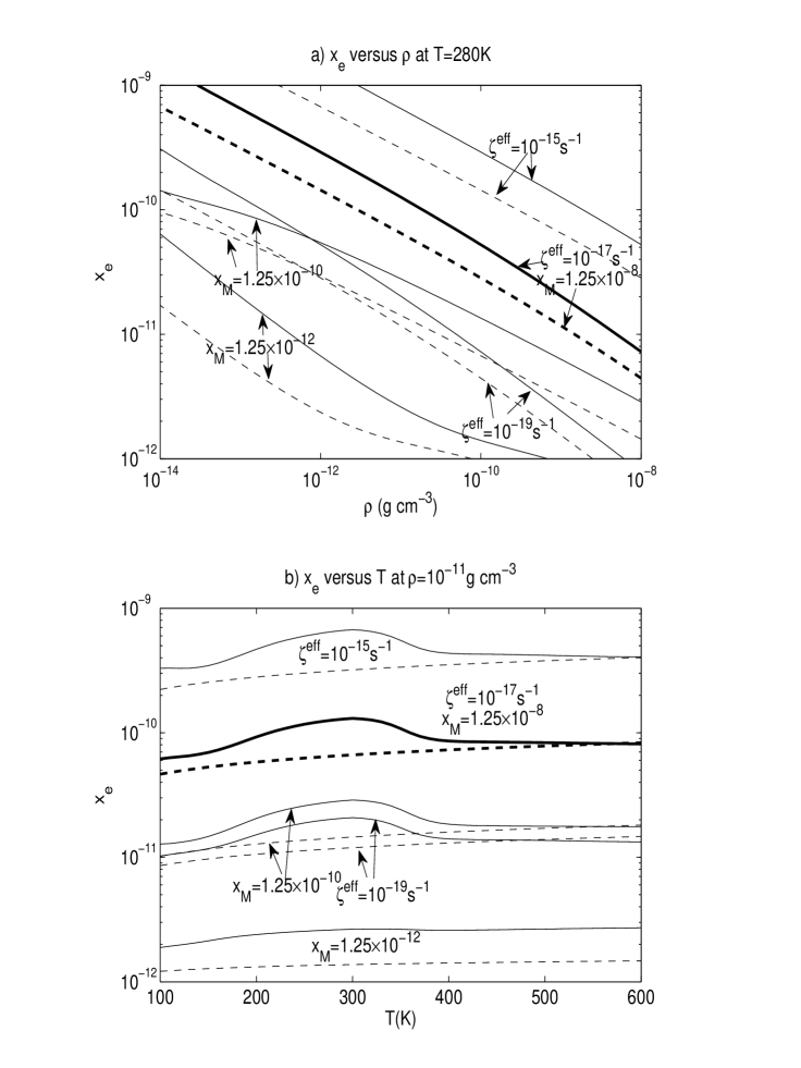
Figure 1: Electron abundance $x_{e}$ in grain-free models. (a) $x_{e}$ versus gas density $\rho$ at constant $T=280{\rm K}$. (b) $x_{e}$ versus $T$ at constant $\rho=10^{-11}{\rm\,g\,cm^{-3}}$ . Dash lines: simple network. Solid lines: complex network. Bold lines are for standard parameters: $\zeta^{\rm eff}=10^{-17}{\rm\,s^{-1}}$, $x_{\rm M}=1.25\times 10^{-8}$. Each of the other curves differs from the standard in one parameter, as shown.

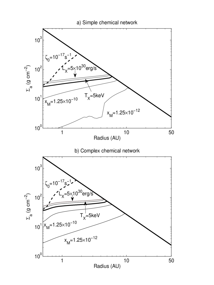
Figure 2: The column density of the active layer defined by $Re_{M}\geq 100$ (§2) versus radius for simple (a) and complex (b) chemical reaction networks without grain particles. The upper bold line indicates the half the total surface density of the disk. The middle bold line corresponds to our standard parameters: $L_{X}=0.5\times 10^{30}{\rm\,erg\,s^{-1}}$, $T_{X}=3{\rm\,keV}$, $\zeta_{0}=0{\rm\,s^{-1}}$, $x_{M}=1.25\times 10^{-8}$. Other curves differ from the standard curve in one parameter, as marked.

4.1.2 Application to the Disk Model

Now temperature and density are fully fixed by the disk model, and our free parameters are ionization rate and metal abundance. The ionization rate is characterized by 3 parameters, namely, X-ray luminosity ($L_{X}$), X-ray temperature ($T_{X}$) and cosmic-ray ionization rate $\zeta_{0}$. Since we already know how metal abundances and ionization rate can affect $x_{e}$, and we also know how ionization parameters affect ionization rate in the disk (see §3.1), our main goal now is to check how these parameters affect the column density of the active layer, $\Sigma_{a}$ (Note that $\Sigma_{a}$ is defined as the active column on one side of the disk). In Figure 2 we plot $\Sigma_{a}$ versus radius. We also compare simple and complex chemical networks in Fig. 2.

Figure 2 shows that in the absence of dust grains, the requirement $\Sigma_{a}\geq 10{\rm\,g\,cm^{-2}}$ (§2) is easily realized. Beyond $2\,\textsc{au}$, the whole disk becomes active once cosmic-ray ionization with $\zeta_{0}\geq 10^{-17}$s^-1 is turned on. Without cosmic-rays, X-rays can also render the whole disk active beyond $6\,\textsc{au}$. In the absence of dust grains, the metal abundance strongly influences the thickness of the active layer. At $1\,\textsc{au}$, reduction of $x_{\rm M}$ from $1.25\times 10^{-8}$ to $1.25\times 10^{-12}$ causes $\Sigma_{a}$ to drop by a factor $10$ for the complex network ($20$ for the simple network). Also, we see that the complex model produces a slightly thicker active zone, consistent with the result in §4.1.1.

4.2 Single-sized Grains

In this subsection, we add a single population of dust grain particles to the chemical reaction network. The standard grain size is $a=0.1\micron$, and the standard mass fraction is $f=0.01$. We evolve the reaction network for $10^{6}$ years.

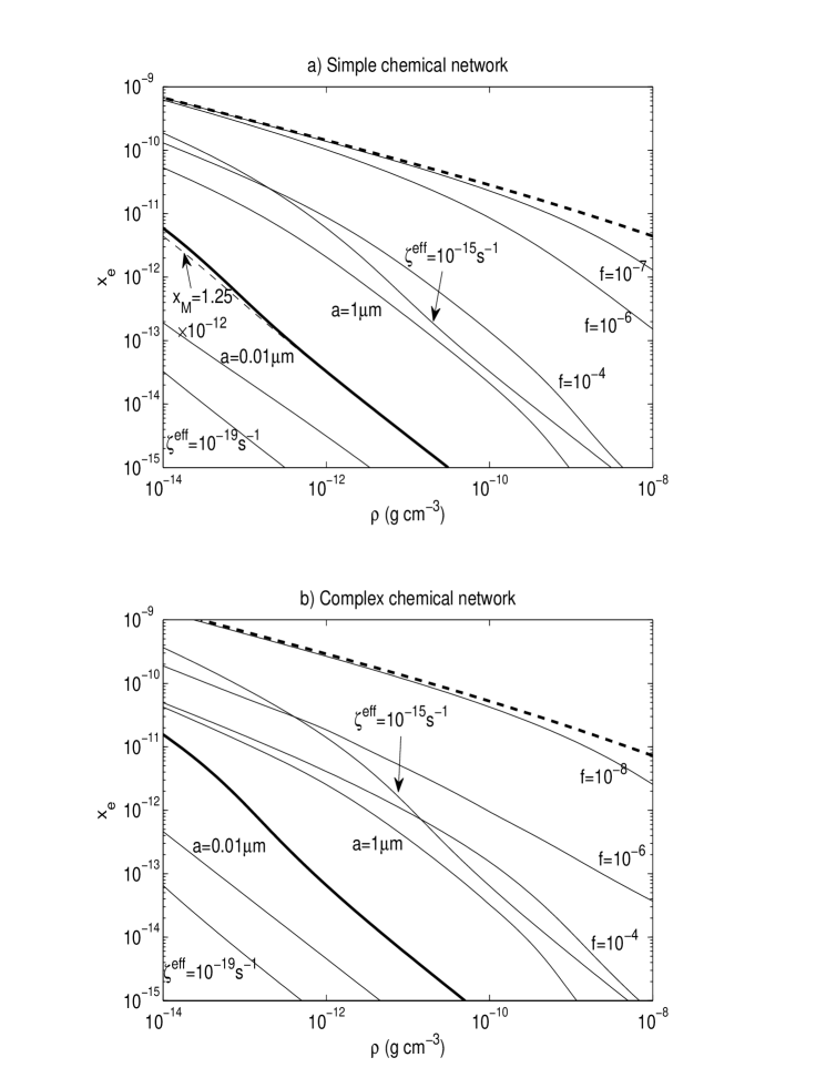
Figure 3: Electron abundance versus gas density at constant temperature, $T=280{\rm K}$ for simple (a) and complex (b) reaction networks with a single population of grains. The bold lines are for the standard values $\zeta^{\rm eff}=10^{-17}{\rm\,s^{-1}}$, $x_{M}=1.25\times 10^{-8}$, $a=0.1\micron$, $f=0.01$, $\eta=10^{-3}$. Other curves differ in one of these parameters, as marked. Bold dashed lines are grain-free ($f=0$). Light dashed line in (a) is for reduced metals, as shown. Note the tiny difference. Panel (b) is even less sensitive to $x_{\rm M}$.

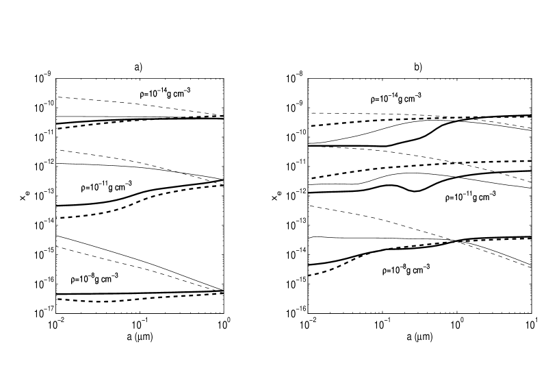
Figure 4: Electron abundance versus grain size with a single population of grains. Solid lines: complex network; dashed lines: simple network. Plots with bold lines have fixed total grain area $f/a=$const, while plots with thin lines keep $f/a^{2}$ constant. Panel (a): Bold lines: $f/a=0.01\micron^{-1}$; thin lines: $f/a^{2}=0.01\micron^{-2}$. (b) Bold lines: $f/a=10^{-4}\micron^{-1}$; thin lines: $f/a^{2}=10^{-4}\micron^{-2}$. Lines in the upper, middle and bottom groups correspond to $\rho=10^{-14}$, $10^{-11}$, and $10^{-8}{\rm\,gcm^{-3}}$ respectively. In all plots, $T=280{\rm K}$, $\zeta^{\rm eff}=10^{-17}{\rm\,s^{-1}}$, $x_{M}=1.25\times 10^{-8}$, $\eta=10^{-3}$. Note that in panel (b) the grain size is extended to $10\micron$

4.2.1 Chemistry

In Figure 3 we plot the free electron abundance as a function of gas density for simple and complex chemical reaction networks respectively. As before, we find that $x_{e}$ scales with density and ionization rate, and is not very sensitive to temperature. There are also some notable differences. Firstly, comparing the bold solid and dashed lines, one sees that with dust grains, $x_{e}$ decreases faster as density increases, suggesting that dust is more effective in suppressing ionization in denser environments. Secondly, comparing Fig. 3 with Fig. 1a, one sees that changing ionization rate by a factor of 100 causes $x_{e}$ to change by less than a factor of 10 in the absence of dust, but by a factor of $25$ in its presence.

A striking difference from the grain-free case is that gas-phase metal atoms are no longer important. This is consistent with what IN06a have found, but our explanation is somewhat different from theirs. At $280{\rm K}$, metal atoms are not swept up by grains (see §3.3.2) at all. Rather, the role that grains play is to promote recombination. We find that when we add grains, the number density of metallic ions is greatly reduced.

With our fiducial parameters, we see that the complex network produces more free electrons, by a factor of $\lesssim 2$. However, as we gradually suppress grains, the simple model recovers the grain-free result more rapidly than the complex model does. In certain ranges, the simple network can produce larger $x_{e}$ than the complex one. For the simple network, reduction of grains by $10^{4}$ ($f=10^{-6}$) is almost enough to recover grain-free result in low density regions, but for complex network, depletion of nearly $10^{6}$ ($f=10^{-8}$) is required.

In Figure 3, we see that electron abundance increases as grains are suppressed, and at fixed grain mass fraction, $x_{e}$ increases with grain size. This is as expected, but grains actually take effect in a complicated way, especially in the complex network, as suggested by the fact that the curves in Fig. 3 are not simply vertical translates of one another. It is natural to ask what combination of $a$ and $f$ best controls $x_{e}$. To investigate this, we plot in Figure 4 $x_{e}$ versus grain size $a$ for a single population of grains at various densities. Plots with bold lines have fixed total surface area $Na^{2}\propto f/a=$const, while for thin lines we have fixed $Na\propto f/a^{2}=$const. If total surface area completely determines $x_{e}$, we would expect that bold lines to be flat. In Fig. 4a, the bold lines for both complex (solid) and simple (dashed) network are approximately flat, and $x_{e}$ slightly decreases as $a$ decreases. This means that total grain surface area is a good approximation to the controlling parameter, though small grains are slightly more effective than big ones. In Fig. 4b, as grains are substantially depleted, we see more complicated dependencies, but with fixed total surface area, the trend is still that $x_{e}$ decreases as $a$ decreases. The fact that small grains are more efficient in reducing $x_{e}$ at fixed total surface area suggests that the controlling parameter may lie somewhere between the total surface area $Na^{2}\propto f/a$ and the combination $Na\propto f/a^{2}$.

The results above can be qualitatively understood. The cross sections of all grain reactions scale with grain surface area, but they are modulated by a grain-polarization term that enhances the cross section of smaller grains. For the reaction $e^{-}+{\rm gr}\rightarrow{\rm gr}^{-}$, the collision rate per grain is proportional to (Draine & Sutin, 1987)

$$\frac{\Gamma_{\rm col}}{\pi a^{2}}\propto 1+\bigg{(}\frac{\pi q^{2}}{2akT}\bigg{)}^{1/2}=1+0.30\bigg{(}\frac{300{\rm K}}{T}\bigg{)}^{1/2}\bigg{(}\frac{1\micron}{a}\bigg{)}^{1/2}$$ (28)

and for $e^{-}+{\rm gr}^{+}\rightarrow{\rm gr}$, the reaction rate is roughly proportional to

$$\frac{\Gamma}{\pi a^{2}}\propto 1+\frac{q^{2}}{2akT}=1+0.056\frac{300{\rm K}}{T}\frac{1\micron}{a}$$ (29)

Although smaller grains also have smaller sticking coefficients for electrons, we find through numerical experiments that over a wide temperature range, the electron sticking coefficient for an $a=1.0\micron$ neutral grain is greater than that for an $a=0.01\micron$ neutral grain by a factor only $\sim 2$. Therefore, the electron abundance is roughly controlled by the total surface area of the dust grains, but smaller grains lead to smaller $x_{e}$ at fixed total surface area.

Our simple analysis here considers just the direct electron absorption by dust grains, which roughly applies to the simple network. For the complex network, however, much more complicated interactions between dust and all the species, as well as the complex reactions in the gas phase make it less predictive. Our numerical experiments above shows that in certain regimes, total surface area controls $x_{e}$, but in other regimes, $na\propto f/a^{2}$ may be a better approximation.

One more comment on the two reaction networks. As mentioned above, $x_{e}$ converges to its grain-free value more rapidly as $f\to 0$ in the simple than in the complex network. This fact is seen more clearly by comparing the left and right panels of Fig. 4. Before grain depletion, $x_{e}$ in the complex network is typically slightly larger than that in the simple network (left panel). As we deplete grains by a factor of 100 (right panel), the simple network typically yields a larger $x_{e}$ than that of the complex network, by up to a factor of 10.

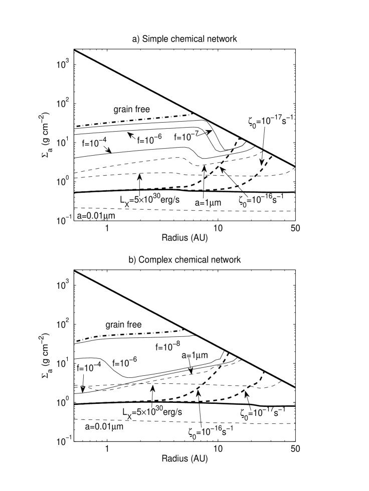
Figure 5: Like Fig. 2, but for a single population of grains with standard values $a=0.1\mu{\rm m}$, $f=0.01$, and $\eta=10^{-3}$. All other parameters at standard values (Table 2) except as indicated. For comparison, we plot the grain-free case in bold dash-dotted lines.

4.2.2 Application to the Disk

Figure 5 plots $\Sigma_{a}$ against radius in the same way as in Fig. 2, and compares different model parameters, especially grain size ($a$) and grain mass fraction ($f$). The column density of the active zone is dramatically reduced when we add sub-micron grains. Both networks predict $\Sigma_{a}\leq 1{\rm\,g\,cm^{-2}}$ at $1\,\textsc{au}$. As in Fig. 3, $\Sigma_{a}$ is more sensitive to ionization than in the grain-free case. X-ray ionization alone cannot ionize the whole disk with our fiducial parameters; but cosmic rays, if unshielded, can ionize the entire column of the outer disk beyond $\sim 10\,\textsc{au}$. These features are also in agreement with Sano et al. (2000).

One sees that $\Sigma_{a}$ has a relatively simple dependence on the grain properties in Fig. 5a (i.e. simple network), but the dependence in Fig. 5b is more complicated. With fiducial parameters, $\Sigma_{a}$ is larger in the complex network, but with reduced dust, the simple network can produce a thicker active layer. Our previous conclusion that total surface area of dust grains roughly controls the electron abundance can be checked in the simple network, where we see that the $a=1\micron$ ($f=0.01$) line is below the $f=10^{-4}$ ($a=0.1\micron$) line. In the complex network, we can see that when $r<0.8\,\textsc{au}$, the $a=1\micron$ line is above the $f=10^{-4}$ line. This corresponds to the situation of Fig. 4b at relatively low densities. Again, the effect of grains on the complex network does not reduce to a single controlling parameter.

In Fig. 5a we see that at about $8\,\textsc{au}$, the two solid lines for $f=10^{-6}$ and $f=10^{-7}$ drop sharply. This corresponds to the sudden depletion of metals onto grains at $T\sim 100{\rm K}$, as discussed in §3.3.2. With less dust (smaller $f$), the transition temperature decreases [see eq. (26)], and the transition radius increases. Outside the transition radius, metals are effectively depleted onto the grains, unless the grain number density is extremely small. In the latter case, our grain adsorption model may fail since the surface of all grains can be fully occupied by adsorbed species. Similar transitions in Fig. 5b (e.g at $f=10^{-6}$ and $f=10^{-8}$) are not well explained by the analysis in §4.2.1.

For the fiducial parameters, metals are not depleted. Under this assumption, we see from Fig. 5 that for $\Sigma_{a}$ to be $\sim 10{\rm\,g\,cm^{-3}}$ at $1\,\textsc{au}$, $a=0.1\micron$ dust grains must be suppressed by a factor $10^{-3}$ ($f=10^{-5}$) for the simple network, and by $10^{-4}$ ($f=10^{-6}$) for the complex network. Suppression by a factor $10^{-5}$ for the simple network and at least $10^{-6}$ for the complex network is need to recover the grain-free case. However, if metals are already depleted (by dust grains), we find that a depletion factor of $10^{-2}-10^{-3}$ is just enough for both the simple and complex network to recover the grain-free result. This can also be seen in Fig. 5 at larger radius where all metals are effectively adsorbed.

The differences between the networks are nontrivial. We cannot recover the results of the complex network by rescaling parameters in the simple one. Therefore a large array of species and reactions may be necessary to calculating the conductivity of protostellar disks.

4.3 Two Grain Sizes

There is no guarantee that the size distribution can be approximated by grains of a single size, because different kinds of reactions (e.g., adsorption and desorption) depend differently on grain size. Therefore, it is necessary to explore the chemistry in protostellar disks using more than one population of grains. On the other hand, the behaviors of grains with different sizes are almost independent. Neglecting grain coagulation, the direct interaction between the two grain populations is via charge exchange, which is slow (see §3.3.1). As a result, we expect to see that $\sum{N_{i}a_{i}^{2}}$ (total grain surface area) or $\sum{N_{i}a_{i}}$ roughly controls the free electron abundance, as we have found in the previous subsection.

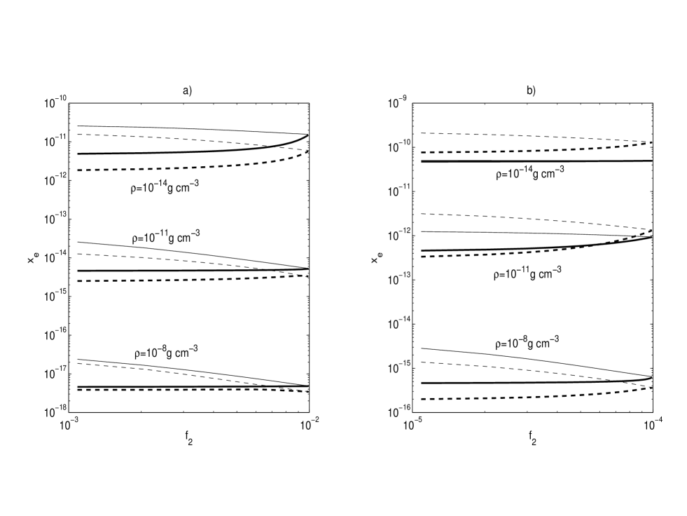
Figure 6: Like Fig. 4 but for two grain populations, $a_{1}=0.01\micron$ and $a_{2}=0.1\micron$. Plots with bold lines have fixed total surface area $f_{1}/a_{1}+f_{2}/a_{2}=$const, while plots with thin lines keep $f_{1}/a_{1}^{2}+f_{2}/a_{2}^{2}$ constant. Shown in the plots are $x_{e}$ versus mass fraction of the larger grains, $f_{2}$. (a). Bold lines: $f_{1}/a_{1}+f_{2}/a_{2}=0.1\micron^{-1}$; thin lines: $f_{1}/a_{1}^{2}+f_{2}/a_{2}^{2}=1.0\micron^{-2}$. (b). Bold lines: $f_{1}/a_{1}+f_{2}/a_{2}=10^{-3}\micron^{-1}$; thin lines: $f_{1}/a_{1}^{2}+f_{2}/a_{2}^{2}=0.01\micron^{-2}$. Note that in the upper part of panel (b), thin and thick solid lines almost overlap.

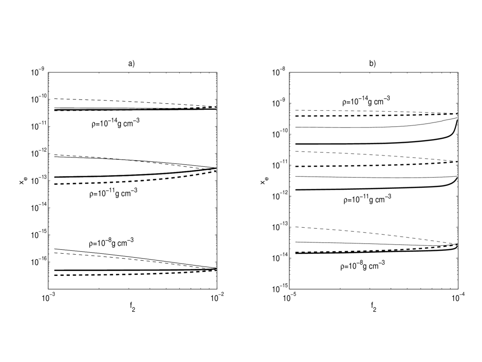
Figure 7: Same as Fig. 6, but the two grain populations are replaced by $a_{1}=0.1\micron$, $a_{2}=1.0\micron$. (a) Bold lines: $f_{1}/a_{1}+f_{2}/a_{2}=0.01\micron^{-1}$; thin lines: $f_{1}/a_{1}^{2}+f_{2}/a_{2}^{2}=0.01\micron^{-2}$. (b) Bold lines: $f_{1}/a_{1}+f_{2}/a_{2}=10^{-4}\micron^{-1}$; thin lines: $f_{1}/a_{1}^{2}+f_{2}/a_{2}^{2}=10^{-4}\micron^{-2}$.

4.3.1 Chemistry

Let $a_{1}$, $f_{1}$ be the size and mass fraction of the smaller grains, $a_{2}$, $f_{2}$ be the size and mass fraction of the bigger grains. Fixed total grain surface area means $N_{1}a_{1}^{2}+N_{2}a_{2}^{2}\propto f_{1}/a_{1}+f_{2}/a_{2}=$const. Fixed $N_{1}a_{1}+N_{2}a_{2}$ means $f_{1}/a_{1}^{2}+f_{2}/a_{2}^{2}=$const. In Figure 6, we consider relatively small grains, $a_{1}=0.01\micron$, $a_{2}=0.1\micron$. As in section 4.2.1, one sees that when grains are fully abundant, and when density is not too low, total grain surface area controls $x_{e}$. In the low density region, and when grains are substantially depleted, the controlling parameter of $x_{e}$ lies in somewhere between $\sum{N_{i}a_{i}}$ and $\sum{N_{i}a_{i}^{2}}$ for the simple chemical network. For the complex network, $\sum{N_{i}a_{i}}$ better controls $x_{e}$ in these regimes. In Figure 7, we consider the two populations of grains to be larger, with $a_{1}=0.1\mu$m, $a_{2}=1.0\mu$m. We see the same trend as before. One notable difference is that for the bold solid lines in Fig. 7b (i.e., complex model at fixed total surface area), there is a sharp increase as $f_{2}\rightarrow 10^{-4}$, or as $f_{1}\rightarrow 0$, especially at low densities. This means that adding a population of smaller grains decreases $x_{e}$ substantially.

In all, the results above confirm the conclusions in §4.2.1. Small grains dominate the free electron abundance, especially in the complex network.

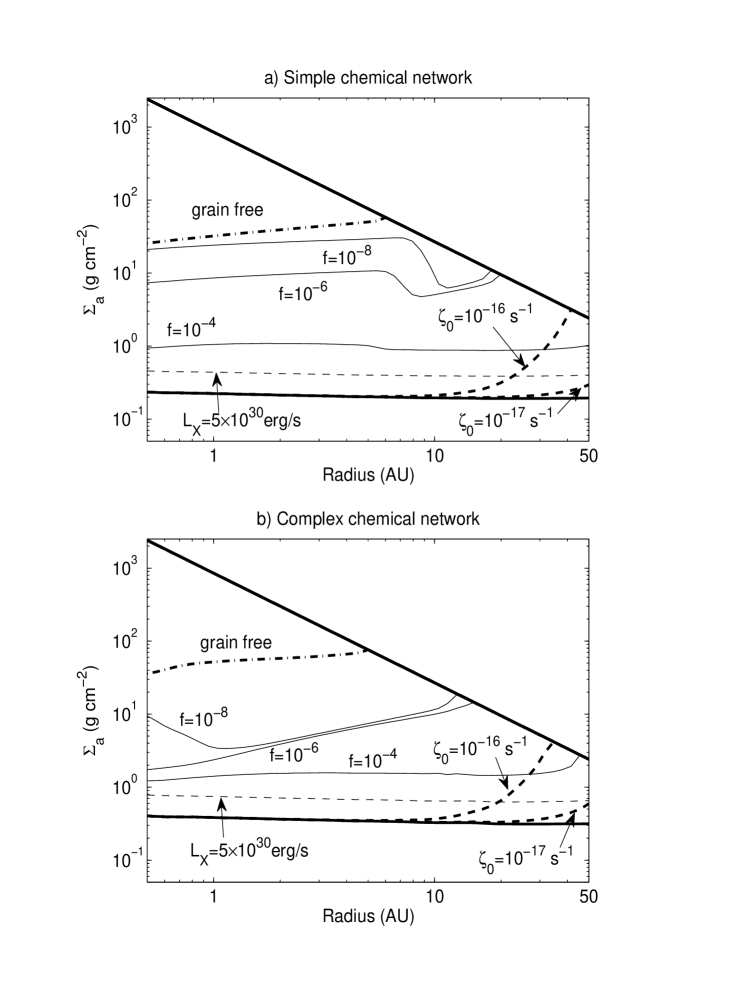
Figure 8: Like Figs. 2 & 5, but for two populations of grains with sizes $a_{1}=0.01\micron$, $a_{2}=0.1\micron$. The mass ratio of the two populations is $f_{1}/f_{2}=(a_{2}/a_{1})^{1/2}=\sqrt{10}$, in rough accord with eq.(23). We use $f=f_{1}+f_{2}$ to represent the total grain mass fraction. All parameters at standard values (Table 2) except as indicated.

4.3.2 Application to the Disk

Figure 8 plots $\Sigma_{a}(r)$ for various parameter choices. One can see that if the dust is fully abundant ($f=10^{-2}$), the thickness of the active layer is appreciably less than $1{\rm\,g\,cm^{-2}}$. For the simple network, a reduction factor $<10^{-4}$ ($f<10^{-6}$) is needed for the thickness of the active zone to reach $10{\rm\,g\,cm^{-2}}$. For the complex network, a reduction factor of $10^{-4}$ can raise $\Sigma_{\rm active}$ to $3{\rm\,g\,cm^{-2}}$, whereas reduction by $10^{-6}$ ($f=10^{-8}$) is still not sufficient to raise $\Sigma_{a}$ to $10{\rm\,g\,cm^{-2}}$. Cosmic-rays hardly affect the ionization of the disk near $1\,\textsc{au}$. The presence of the smallest dust grains ($a=0.01\micron$) demands a very high ionization rate of the order $\zeta^{\rm eff}\sim 10^{14}$ to achieve $\Sigma_{a}=10{\rm\,g\,cm^{-2}}$ for standard values of the other parameters. This is excessively high for interstellar cosmic-rays but might perhaps be produced by nonthermal processes (reconnection?) within the corona of the disk or the protostar.

We conclude that when we account for the smallest grains, the column density of the active zone is dramatically reduced. In order that the active column $\Sigma_{a}$ be large enough to support vigorous accretion, the smallest grains must be severely suppressed. In the complex network, $x_{e}$ is more sensitive to the smallest grains, and more drastic depletion is needed. Our results show that $0.01\micron$ grains should be almost completely removed, and $0.1\micron$ ones should be reduced by a factor of $10^{4}$ compared to interstellar abundances.

5 Molecular cooling of the active layer

If accretion is driven by turbulent angular-momentum transport within the disk, then in steady state, the heat released per unit area from each side of the disk is (Pringle, 1981) $\dot{Q}\approx 3\dot{M}\Omega^{2}/8\pi$; the corresponding effective temperature is

$$T_{\rm eff}\approx 150\,\dot{M}_{-7}^{1/4}r_{\,\textsc{au}}^{-3/4}\,{\rm K}.$$ (30)

The heat of wind-driven accretion would be less, because of the mechanical energy carried by the wind itself. At a normal interstellar gas-to-dust ratio, the heat of accretion would be radiated primarily by the dust. However, as we have seen, the dust abundance must be substantially lowered in the active layer in order that the conductivity of the layer be sufficient to couple it to the magnetic field. It is possible that the dust is so strongly depleted that the layer becomes optically thin. In that case, molecular lines might be seen in emission from the layer.

In fact, Salyk et al. (2008) have observed $\,{\rm H_{2}O}\,$ emission in the $10-20\micron$ (with Spitzer-IRS) and $3-5\micron$ (with Keck-NIRSPEC) wavelength regions in two T Tauri systems with particularly high accretion rates of order $10^{-6\pm 1}{\rm M_{\sun}\,yr^{-1}}$, DR Tau and AS 205. These authors infer that the emitting gas lies at $\sim 1\,\,\textsc{au}$ from the central star in both systems and has a temperature $\sim 10^{3}\,{\rm K}$. This is probably too hot to represent the active layer as a whole unless its optical depth is as small as $\tau<10^{-2}$ (note $T_{\rm gas}\approx\tau^{-1/4}T_{\rm eff}$ if $\tau<1$). Indeed, their analysis suggests a surface density $\lesssim 0.1\,{\rm g\,cm^{-2}}$ for the emitting gas, assuming a cosmic abundance of oxygen in the form of $\,{\rm H_{2}O}\,$. So the emission may be coming from tenuous UV-heated gas well above the active layer. Nevertheless, these observations further motivate us to consider the possibility of significant molecular emission from active layers.

In order that the molecular lines should dominate the cooling, however, the active layer must be more than modestly optically thin to dust, that is to say, it must be that $\tau_{\rm d}\ll 1$. The reason is that, in contrast to the situation in planetary or stellar atmospheres, the molecular lines are significantly narrower than their separation, so that they cover only a small fraction of the infrared spectrum. In other words, the emissivity of the active layer due to molecular lines is expected to be small. The rest of the present section is devoted to quantifying this statement via a representative calculation.

Since we are not attempting to fit actual data but only to indicate what might be expected to be emitted by a theorist’s notional active layer, we consider $\,{\rm H_{2}O}\,$ only. This is probably the most important molecular coolant because it is expected to be abundant, being composed of two of the most abundant elements and being strongly thermodynamically stable under these physical conditions, and because it has a much richer rotational spectrum than the common linear molecules ${\rm CO}$ and ${\rm CO_{2}}$. For similar reasons, ammonia (${\rm NH_{3}}$) may be almost as important as water as a coolant. Because of the terrestrial significance of water vapor, the molecular spectrum of $\,{\rm H_{2}O}\,$ is particularly well studied. We have relied mainly on the extensive line and energy-level lists of (Barber et al., 2006, hereafter BT), but we have also consulted the JPL Molecular Spectroscopy database and obtained consistent results for the molecular emissivity at $T_{\rm gas}=300\,{\rm K}$; however, the JPL database omits lines with wavelengths $<10\micron$, whereas $\sim 25\%$ of a blackbody emits shortward of that cutoff even at $300\,{\rm K}$, and of course a larger fraction at higher temperatures.

For simplicity, we represent the active layer by an isothermal slab in LTE at gas temperature $T$ and define its emissivity by

$$\epsilon\equiv\frac{1}{\sigma T^{4}}\int\limits_{0}^{\infty}\left(1-e^{-\tau_{\nu}}\right)\pi B_{\nu}(T)\,d\nu\,,$$ (31)

where $\tau_{\nu}$ is the frequency-dependent optical depth due to water alone, which in turn is related to the water column $N$ (in molecules cm^-2), the line “intensities” $I_{k}$ (in cm molecule^-1), and the line broadening function $\phi_{k}(\Delta\nu)$ (in cm) by

$$\tau_{\nu}=N\sum_{k}I_{k}\phi_{k}(\nu-\nu_{k}).$$ (32)

Following the molecular spectroscopists’ convention, the frequency $\nu$ is measured in wavenumbers (cm^-1) rather than Hertz. We take $N/\Sigma_{\rm a}=3.6\times 10^{20}\,{\rm molecules\,g^{-1}}$, which corresponds to the abundances of Anders & Grevesse (1989) if all of the oxygen is in water. The relationship between the line intensity $I$ and the Einstein coefficient $A_{if}$ is temperature dependent and is given for LTE by eq. (3) of BT.

In the limit of low columns where all lines are unsaturated ($\tau_{\nu}\ll 1$) eq. (31) would reduce to

$$\epsilon_{\rm a}=\frac{N}{\sigma T^{4}}\sum_{k}I_{k}B_{\nu}(T)\,,$$ (33)

This becomes $2.17\times 10^{-20}\,N$ at 300 K, corresponding to a Planck-mean opacity $\kappa_{\rm Pl}\approx 7.8\,{\rm cm^{2}\,g^{-1}}$. Since the emissivity cannot exceed unity, it is clear that the important lines must saturate at $\Sigma_{\rm a}>\kappa_{\rm Pl}^{-1}\approx 0.13\,{\rm g\,cm^{-2}}$, and in fact the stronger lines saturate at even lower columns because under the conditions of interest, the lines are very narrow. Thus, for an active layer of surface density $\sim 10\,{\rm g\,cm^{-1}}$, the actual emissivity defined by eq. (31) will be sensitive to the broadening prescription, which therefore merits some discussion.

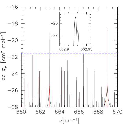
Figure 9: Frequency-dependent absorption cross-section per water molecule over a small range of wavenumbers $\nu=\lambda^{-1}$ at $T=300\,{\rm K}$ and $P=1\,{\rm\mu bar}$. Red curve: Thermal Doppler broadening only. Black: Doppler plus collisional broadening. Horizontal dashed line shows level above which lines would be saturated for a total mass column of $10\,{\rm g\,cm^{-2}}$ assuming a solar abundance of oxygen in ${\rm H_{2}O}$, i.e. $3.6\times 10^{20}\,{\rm molecules\,g^{-1}}$. Inset shows a closeup of two overlapping lines; but note that one is relatively weak.

The relative sizes of the natural width $\Delta\nu_{0}$, the collisional width $\Delta\nu_{c}$, the thermal Doppler width $\Delta\nu_{D}$, and the turbulent width $\Delta\nu_{T}$ (all of these are defined as half widths at half maximum) depend upon the temperature, pressure, and turbulent intensity. The temperatures of interest to us are within a factor of a few of that in the Earth’s atmosphere, $T\sim 300\times 10^{\pm 0.5}\,{\rm K}$, but the pressures are much lower. If the base of the active layer lies at a height $z_{\rm a}\ll r$ above the midplane, then the pressure there is $P_{\rm a}\approx\Sigma_{\rm a}\Omega^{2}z_{\rm a}$; if $z_{\rm a}\approx 3[k_{\textsc{b}}T/m(H_{2})]^{1/2}\Omega^{-1}$, i.e. three times the gaussian scale height of the disk (note that $T$ here should be the temperature near the midplane, which may be somewhat lower than in the active layer), then

$$P_{\rm a}\approx 0.7\,\left(\frac{\Sigma}{10\,{\rm g\,cm^{-2}}}\right)\left(\frac{T}{300\,{\rm K}}\right)^{1/2}\,{\rm dyn\,cm^{-2}}\,;$$ (34)

in other words, we are interested in pressures of order one microbar or less $(10^{6}\,{\rm dyn\,cm^{-2}}=1\,{\rm bar})$. The natural width

$$\Delta\nu_{0}=\frac{1}{4\pi}\sum_{f}A_{if}\,,$$ (35)

is $<3$ Hz (i.e., $<10^{-10}\,{\rm cm^{-1}}$ in wavenumbers) for all upper levels $i$ tabulated by BT whose energies are less than $(3000\,{\rm K})k_{\textsc{b}}$ above the ground state. This is completely negligible compared to the other causes of line broadening; in particular, it is much smaller than the collisional width, which justifies our assumption of LTE. Neither BT nor the JPL database give collisional widths. These are difficult to calculate precisely and are well-measured for only a minority of transitions. For our purposes, it will be enough to have a rough estimate, so for all lines we use

$$\Delta\nu_{c}=0.075\,\left(\frac{P}{\rm bar}\right)\left(\frac{T}{300{\rm K}}\right)^{-1/2}{\rm cm^{-1}}\,,$$ (36)

based on the value quoted by Townes & Schawlow (1955) for NH₃ (not $\,{\rm H_{2}O}\,$) in ${\rm H_{2}}$. For comparison, Giesen et al. (1992) find $\Delta\nu_{c}=0.086\pm 0.002\,{\rm cm^{-1}\,bar^{-1}}$ for $\,{\rm H_{2}O}\,$ in N₂ at $296\,{\rm K}$. Thus, even at $P\sim 1\,{\rm\mu bar}$, $\Delta\nu_{c}\gtrsim 10^{3}\Delta\nu_{0}$ for the important transitions. So we have neglected the natural widths. The thermal Doppler width of a line with central frequency $\nu_{k}$ is

$$\Delta\nu_{D}=\sqrt{2\ln 2}\left(\frac{k_{\textsc{b}}T}{m(\,{\rm H_{2}O}\,)\,c^{2}}\right)^{1/2}\nu_{k}\approx 1.46\times 10^{-3}\left(\frac{T}{300\,{\rm K}}\right)^{1/2}\left(\frac{\nu_{k}}{1000\,\rm cm^{-1}}\right)\,{\rm cm^{-1}}\,.$$ (37)

This is typically two orders of magnitude smaller than the collisional width under terrestrial conditions, but at the much lower pressures of an active layer, Doppler broadening should dominate by a large factor: $\Delta\nu_{D}\sim 10^{4}\Delta\nu_{c}$. Nevertheless, the collisional broadening is not entirely negligible for us because it produces an approximately Lorentzian profile whose wings exceed those of the thermal Maxwellian far from the line center, and which can yield significant emission from the most strongly saturated lines. Finally, while the turbulent width is uncertain because of uncertainties in the strength and nature of the turbulence itself, for MRI-driven accretion we expect that the turbulent Mach number should be $\lesssim 0.5[\alpha k_{\textsc{b}}T/m({\rm H_{2}})]^{1/2}$. This is less than the thermal width unless the viscosity parameter $\alpha\gtrsim 0.5$, which seems unlikely in these rather resistive circumstances. On these grounds, we have neglected the turbulent width. But it should be borne in mind that the turbulent velocity fluctuations might be significantly nongaussian if the turbulence is intermittent, in which case the wings of the turbulent velocity profile might contribute importantly to the emission from the more saturated lines. Figure 9 demonstrates the effects of Doppler and collisional broadening on the frequency-dependent molecular absorption cross section, $\sigma_{\nu}$; if it were due entirely to water, the corresponding opacity would be $\kappa_{\nu}=\sigma_{\nu}N_{A}X({\rm H_{2}O})/m({\rm H_{2}O})$, where $X({\rm H_{2}O})$ is the abundance of water by mass, and $m({\rm H_{2}O})\approx 18m_{p}$ is the mass per molecule. At the very low pressures (by comparison with atmospheric or stellar conditions), relatively low temperatures, and modest columns relevant here, the strong and saturated lines rarely overlap. The Doppler-broadened spectrum (red online) shown in the figure was produced with the code spectra-bt2 of BT, and then convolved with a Lorentzian to simulate collisional broadening.

Figure 10: Cumulative emissivity of dust-free isothermal slabs due to water. Solid curves: $\Sigma=10\,{\rm g\,cm^{-2}}$; dotted: $1\,{\rm g\,cm^{-2}}$. Top to bottom at right: $T=600,450,300,150{\rm K}$.

Figure 10 shows the cumulative emissivity defined by the incomplete integral corresponding to eq. (31),

$$\epsilon(<\nu)\equiv\frac{\pi}{\sigma T^{4}}\int\limits_{0}^{\nu}\left(1-e^{-\tau_{\nu^{\prime}}}\right)B_{\nu^{\prime}}(T)\,d\nu^{\prime}\,,$$ (38)

for isothermal slabs representative of notional active layers. Evidently, the molecular emissivity of active layers is expected to be $\ll 1$, but perhaps not negligible compared to dust if the latter is as strongly depleted as good magnetic coupling requires. The sublinear dependence on column density demonstrates that the emissivity is dominated by saturated lines.

We have found that eq. (38) cannot be calculated reliably using the frequency-dependent opacities of Sharp & Burrows (2007) because these were intended for use in stellar and planetary atmospheres where collisional broadening is far stronger than in disks: the saturation of the stronger lines is therefore underestimated, so that the resulting emissivities are typically several times larger than those shown in Fig. 10. We have not tried to use the even more recent tabulations of Freedman et al. (2008) but would expect similar difficulties, since those opacities were computed for minimum pressures of $300\,{\rm\mu bar}$. Rather than construct our own tables of $\kappa_{\nu}$ with the required resolution (finer than $\Delta\nu_{D}/\nu\sim 10^{-6}$), we have exploited the fact that the important lines are well separated to replace eq. (38) with a line-by-line sum that properly accounts for the broadening and saturation of the individual lines:

$$\epsilon(<\nu)\approx\frac{\pi}{\sigma T^{4}}\,\sum\limits_{{\rm lines}~{}k}B_{\nu_{k}}(T)\int\limits_{0}^{\nu}\left\{1-\exp\left[-NI_{k}\phi(\nu^{\prime}-\nu_{k})\right]\right\}\,d\nu^{\prime}\,,$$ (39)

It is easily seen that eq. (39) strictly overestimates eq. (38) to the extent that lines overlap. But direct comparisons using limited wavenumber ranges indicate that the relative error of the line-by-line sum (39) is small ($\ll 10^{-2}$) at our pressures and temperatures.

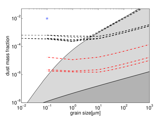
Figure 11: Constraints on grain size distribution and abundance in the MMSN at 1 AU. Abscissa is grain radius $a_{0}$ for single-size models, $N(a)\propto\delta(a-a_{0})$, or $a_{\max}$ for MRN power-law size distribution (23) with $a_{\min}=0.01\micron$. Light solid line: Conductivity constraint for single-size grains, derived using the complex network with $\Sigma_{a}=10$g cm^-2; allowed models lie below line, shaded in light grey. Heavy solid line: Corresponding constraint for MRN size distribution, using the effective grain mass fraction of the smallest grains in equation (40). Allowed region is shaded in dark grey. Light long-dashed lines: Loci of optical depth $\tau_{\rm dust}=1$ for single-sized grains in active layer with $\Sigma_{\rm gas}=10\,{\rm g\,cm^{-2}}$ and $T_{\rm gas}=150,300,600\,{\rm K}$ from top to bottom at left. Heavy long-dashed lines: Corresponding loci for MRN models. Dash-dotted lines: Corresponding loci for equal frequency-averaged dust and ${\rm H_{2}O}$ emissivities, assuming MRN dust size distribution. Asterisk: Typical ISM values.

5.1 Implication of conductivity constraints for molecular lines

Figure 11 summarizes our constraints on the dust in the plane of dust abundance ($f$) versus grain radius ($a$), for single-sized grains, or maximum grain radius ($a_{\max}$) for power-law size distributions, $n(a)da\propto a^{-3.5}da$. The conductivity constraint is based on the complex chemical network, with single species calculations. Parameters that lead $\Sigma_{a}\geq 10$g cm^-2 are considered as allowed. For the power-law size distribution, we have not tried to reproduce the complexities seen in Figures 7-8. The calculations show that the dependencies of the free-electron abundance, $x_{e}$, and of the column density of the active layer, $\Sigma_{\rm a}$, are not accurately given by power laws in the dust-to-gas ratio ($f$) or grain radius ($a$). However, Figures 5, 6, & 7 do suggest that at gas densities relevant to the base of the active layer ($\rho\sim 10^{-11}{\rm g\,cm^{-3}}$), it is roughly the case that $x_{e}$ varies with $f^{\prime}(a)$ and $a$ in the combination $\int{daf^{\prime}(a)/a^{p}}$ with an exponent $p$ somewhere between $1$ and $2$, where $f^{\prime}(a)\propto a^{3}N(a)$ is the differential mass fraction of grains with size $a$. Therefore, for the purposes of Fig. 11, we have taken $\int_{a_{\min}}^{a_{\max}}{daf^{\prime}(a)/a^{p}}$ as the controlling parameter for the conductivity, with $p=3/2$. To account for the power-law models with the MRN size distribution, we use a single-size grain model at the minimum grain size $a_{\min}$ with an effective mass fraction

$$f(a_{\min})=\frac{(a_{\min})^{3/2}\int_{a_{\min}}^{a_{\max}}a^{-2}da}{\int_{a_{\min}}^{a_{\max}}a^{-1/2}da}f=\frac{a_{\min}+\sqrt{a_{\min}a_{\max}}}{2a_{\max}}f\ .$$ (40)

The minimum radius is fixed at $a_{\min}=0.01\micron$, which we believe to be conservative: if grains as small as this do exist in the active layer, then even smaller ones are probably present—perhaps all the way down to the PAH regime $a\sim 10\mbox{\AA}$—and such very small grains may dominate the conductivity. However, we have not calculated any ionization networks for grains smaller than $0.01\micron$. Values of $a_{\max}$ larger than $10^{3}\micron=1\,{\rm mm}$ are not shown in Fig. 11 because our own rough estimates suggest that larger grains would precipitate out of the active layer even in the presence of residual turbulence in the underlying “dead” zone at the level $\alpha_{\rm dz}\approx 10^{-5}$, a value that we deduce from (grain-free) simulations (Turner et al., 2007; Oishi et al., 2007; Turner & Sano, 2008).

Also shown in Figure 11 are the loci at which an active layer of surface density $\Sigma_{\rm a}=10\,{\rm g\,cm^{-2}}$ would be marginally optically thick to to dust, and the much lower loci at which the emissivities of the layer due to ${\rm H_{2}O}$ and dust would be comparable. The dust opacities were derived from the thermally-averaged optical efficiency factors computed by Draine & Lee (1984); we assumed a mixture of 58% silicate and 42% graphite grains by mass. The Figure shows that the absorption opacity depends mainly on dust mass fraction provided $a_{\max}\lesssim 3\micron$, because emission and absorption then occur mainly in the dipole regime. The $\tau_{\rm dust}=1$ curves are also rather insensitive to the temperature, at least over the range we consider ($150-600\,{\rm K}$). The equal-emissivity curves are more sensitive, however, because of the temperature dependence of the molecular emissivity seen in Fig. 10.

The main conclusion that we draw from Figure 11 is that the active layer should be optically thin to dust. Therefore molecular emission lines should stand out above the dust continuum if the layer is heated by dissipation of MRI turbulence. The detectability of the lines will be reduced by the Doppler broadening associated with the orbital motion of the gas, which is much larger than thermal and collisional broadening, unless the disk is observed face on or spatially resolved (e.g. with an interferometer). The upper solid line shows that if grains smaller than $a\sim 1\micron$ are entirely absent, then there does exist a regime in which $\tau_{\rm dust}>1$ despite the ionization being sufficient for good coupling. The lighter solid and dashed lines show that if grains smaller than $a\sim 1\micron$ are entirely absent, then there does exist a regime in which $\tau_{dust}\approx 1$ despite the ionization being sufficient for good coupling. In the more plausible situation described by the power-law models, where small grains occur but in reduced abundance compared to ISM values, due both to growth of the largest grains and to reduction (or precipitation) of the overall dust mass fraction, the conductivity constraint requires $\tau_{\rm dust}\ll 1$. It seems even to require that cooling of the active layer is dominated by molecules rather than dust, unless grains smaller than $\sim 0.1\micron$ are essentially completely excluded.

6 Discussion

The preceding sections have shown that our understanding of the interplay among grains, magnetic fields, and thermal emissions in protostellar disks suffers from many uncertainties. Some of these uncertainties might be reduced in the foreseeable future by further research. Others seem likely to plague astronomers for quite some time.

6.1 Uncertainties in the Conductivity Calculation

Our criterion of the active zone is based on the choice of the critical magnetic Reynolds number ${\rm Re}_{M}^{\rm crit}=100$. As discussed in §2, our estimate may be conservative, and our calculation may provide the upper limit of the size of the active zone.

We have adopted the minimum-mass solar nebular disk model. This model is idealized in two aspects. It has an empirical surface density profile designed to match the mass distribution in the solar system. In the MMSN, the mass density scales linearly with the surface density coefficient $\Sigma_{0}$, but the disk scale height is independent of $\Sigma_{0}$, and therefore so is the flux of X-rays and cosmic-rays impinging on the disk. In fact, we have experimented with different $\Sigma_{0}$, and found that $\Sigma_{\rm a}$ is essentially independent of $\Sigma_{0}$, although at higher surface density, the active layer of the disk resides at higher altitude. The MMSN is also assumed to be vertically isothermal. In reality, in the presence of small grains, the surface layers should be warmer than the midplane even in a disk passively heated by stellar irradiation (Chiang & Goldreich, 1997, 1999), and warmer still if turbulent accretion is concentrated in active layers. Higher temperature reduces the recombination rate and thereby increases the electron abundance, but only weakly ($\propto T^{-1/2}$, see §4.1.1). Therefore, we expect that the size of the active zone is not affected much by the disk temperature profile. Molecular emission, however, could be strongly affected (§5).

Major uncertainties attend the ionization model. The ionization rate is proportional to the X-ray luminosity and also depends on the X-ray temperature of the bremsstrahlung spectrum. A stellar wind may shield cosmic rays from the disk. In the outer disk, X-ray ionization is inefficient when small dust grains are present, and the ionization rate critically depends on cosmic rays. These effects are well studied in this paper. A related uncertainty comes from metal abundances. Metal atoms are effective electron donors. In the absence of grains, the electron abundance is directly correlated with metal abundance. Since our results show that grains must be severely suppressed in order for a reasonable amount of the disk to be active, under such conditions, metals may be important. Our standard parameter assumes a relatively high metal abundance ($x_{M}=1.25\times 10^{-8}$). Our results also suggest that the abundance is unlikely to be much lower than this, since an even more severe constraint on the dust abundance would then be required. Moreover, in the outer disk where the disk temperature is low, essentially all the metals are adsorbed onto dust grains. Unless cosmic-rays can provide the ionization, the outer disk is unlikely to be very active.

Grain properties are another major source of uncertainty, as studied in detail in this paper. We devote the next subsection discussing the grain size distribution. Here, we emphasize that the simple and complex reaction networks show different response to grain abundance. Namely, in the complete absence of grains, or at the full ISM dust-to-mass ratio ($f=0.01$), the complex network produces more free electrons. However, for intermediate dust abundances, the simple network gives a larger $x_{e}$, sometimes even 10 times larger. The Oppenheimer & Dalgarno model, though popular for its simplicity (eg.Turner & Sano, 2008), should therefore be used with caution when grains are assumed.

6.2 Grain size distribution

The basic theme of this paper is to compare constraints on the grain abundance from the requirement of adequate magnetic coupling to those provided by infrared observations of thermal disk emission. For a given total mass $f$ in grains per unit mass of gas, however, these two constraints depend differently on the sizes of grains, to the point that no useful comparison can be made if the size distribution is regarded as a completely free function. Thus, it is important to consider what constraints are available for this distribution. To bound the discussion, we take the distribution to be a truncated power law similar to the standard MRN form (23) but possibly with different lower and upper cutoffs ($a_{\min}$ and $a_{\max}$) and with a different exponent $p$, i.e. $N(a)\propto a^{-p}$.

Collisional cascades involving macroscopic bodies such as asteroids or Kuijper-Belt objects result in powerlaws with $p\approx 3.5$ when the cohesive strength is independent of size; the slope becomes steeper (i.e. larger $p$) if large bodies are weaker than small ones, and shallower in the opposite case (O’Brien & Greenberg, 2005, and references therein). In line with this, Jones et al. (1996) have proposed that the MSN distribution results from collisions between grains overrun by shocks. In their model, the grains are taken to have strengths similar to those terrestrial rocks and minerals, so that the minimum relative velocity between grains required for fragmentation is $1\,{\rm km\,s^{-1}}$. This is much larger than the likely collisional velocities of submicron grains in protostellar disks.

Many authors have considered the collisional agglomeration of grains in protostellar disks. In a recent study, Dullemond & Dominik (2005) demonstrate that if the sticking probability is taken to be high and fragmentation is ignored, then almost all grains smaller than $a\sim 100\,\micron$ would disappear in less than $10^{4}\,{\rm yr}$, causing the disks to become optically thin. As they note, this contradicts the observation that many or most T Tauri disks remain optically thick, as judged by their spectral energy distributions at $10-100\,\micron$, to ages of at least $10^{6}\,{\rm yr}$; the suggestion is that small grains must be replenished by fragmentation processes.

In a recent review, Natta et al. (2007) discuss the observational evidence for grain growth and grain processing in protostellar disks. Millimeter observations indicate the presence of millimeter or even centimeter-sized grains in many disks. On the other hand, infrared silicate features—especially crystalline features near $10\micron$—point to the persistence of micron or submicron-sized grains even in the oldest disks. PAH features are also sometimes seen. But there is no clear evolutionary trend in the grain size distribution with disk (or rather stellar) age, which points again to active replenishment of the small-grain population.

6.3 Turbulent Mixing

We have calculated the free-electron abundance and conductivity as a function of local parameters: density, temperature, grain abundance, and ionization rate, etc. Since X-rays and cosmic rays penetrate only a limited column, the resulting electron abundance has a large vertical gradient. Any turbulent diffusion would mix electrons and ions vertically. The consequences for the width of the active layer depend upon the ratio of the timescales for mixing and recombination. If accretion is driven by turbulence and the turbulent transport coefficient for mass is comparable to that for momentum (i.e. to the turbulent viscosity), then absent dust grains, the diffusion may be faster than recombination; as a result, the dead zone may be reduced or even eliminated (Ilgner & Nelson, 2006b).

Recently, Turner et al. (2007) performed 3D MHD simulations of protostellar disks with vertical structure, Ohmic resistivity, and time-dependent chemical evolution based on the simple (Oppenheimer-Dalgarno) reaction network without grains, allowing the reactants to be passively advected. Turbulent mixing led to a weak coupling of the dead zone to the magnetic field. Ilgner & Nelson (2008) found in similar simulations that the effect of turbulent mixing critically depend on gas-phase metal abundance. Turner & Sano (2008) included a uniform mass fraction of $1\micron$ dust grains. Despite rapid recombination on grain surfaces, the radial magnetic field generated in the active layer diffused toward the disk mid-plane, causing some accretion there and rendering it “undead”.

The simulations cited above adopted microphysical parameters very favorable to MRI. For example, in the absence of grains, as in Turner et al. (2007) and Ilgner & Nelson (2008), atomic metal ions recombine only by radiative processes, which are slow compared to the dissociative recombination of molecular ions. The 1$\micron$ grains adopted in Turner & Sano (2008) affect the electron abundance much less than smaller grains, as we have seen. Ilgner & Nelson (2008) chose a rather high protostellar X-ray luminosity ($10^{31}{\rm erg\,s^{-1}}$) and temperature ($5\,{\rm keV}$) . While all of these simulations would be described as “vertically stratified” in the parlance of MRI shearing-box work because they included vertical gravitational accelerations, buoyancy forces were excluded by the use of isothermal equations of state. True stratification, as expected in real disks, may inhibit vertical mixing.

Most importantly, the relevant component of the turbulent stress, $T^{r\phi}$, was found to be at best constant with height. Since, in steady state accretion, the accretion rate is proportional to the areal integral of this stress [see eq. (14)], the “undead” zones contribute to $\dot{M}$ only in proportion to their geometrical thickness, which is comparable to that of the active layers, rather than in proportion to their mass column.

7 Summary and Conclusion

We have studied constraints on small dust grains in protostellar disks posed by the requirement that the electrical conductivity be sufficient to support magnetically driven accretion at observed rates. We have considered the implications of these constraints for the production of molecular emission lines, especially at radii $\sim 0.1-10\,\textsc{au}$ where accretion is likely to to be confined near the surfaces of the disk in “active” layers comprising a fraction of the total column density. We adopt the minimum-mass solar nebular (MMSN) and assume protostellar X-rays and interstellar cosmic-rays to be the main sources of ionization. We compare a simple chemical reaction modeled on Oppenheimer & Dalgarno (1974) with a complex reaction network extracted from the latest UMIST database (Woodall et al., 2007). Reactions involving dust grains are modeled according to the general scheme laid out by Ilgner & Nelson (2006a, hereafter IN06a), with some improvements, including the use of up to two grain sizes in order to mimic an MRN grain size distribution. The conductivity is heavily dominated by the smaller grains. We discuss in detail the dependence of free electron abundance ($x_{e}$) on density, temperature, ionization rate, gas-phase metal abundance, and especially on grain size and grain abundance.

Separately, we estimate that electron fractions $x_{e}\gtrsim 10^{-11}\mbox{-}10^{-10}$ are required at $1\,\textsc{au}$ to explain accretion at $10^{-7}M_{\odot}{\rm yr^{-1}}$, which is typical of the more active systems; minimum magnetic field strengths range from a few tenths of a Gauss if accretion is driven by winds, to several gauss if it is powered by magnetorotational turbulence. It is difficult to be very precise about these requirements because of the complexities of winds and turbulence in the presence of vertical stratification and tensorial conductivities, but the numbers just given are probably conservative. We define the active layer as the column density $\Sigma_{a}$ at which $Re_{M}\geq 100$, where $Re_{M}\equiv c_{s}/\Omega\eta$ and $\eta$ is the Ohmic diffusivity. Smaller values of $Re_{M}$ are probably not realistic because, at the field strengths we estimate, Hall and ambipolar drift contribute to slippage between the neutrals and the field. By this definition, it is difficult to achieve $\Sigma_{a}\geq 10\,{\rm g\,cm^{-2}}$ at $1\,\textsc{au}$ even if the small grains are strongly suppressed.

In more detail, our conclusions regarding the conductivity are as follows:

1. The free electron abundance $x_{e}$ depends more strongly on density ($\rho$) and ionization rate ($\zeta$) than on temperature. Even a small amount of dust suppresses atomic ions such as ${\rm Mg^{+}}$ and ${\rm Fe^{+}}$ in the gas phase, as found by Ilgner & Nelson (2006a); however, we find that this is due to recombination on grain surfaces rather than adsoprtion, except at temperatures ($\lesssim 100K$ for Mg).

2. In the absence of grains, the complex chemical reaction network predicts a slightly higher $x_{e}$ than the simple Oppenheimer-Dalgarno model, rather than the reverse as IN06a found. This appears to be caused by updates to the reaction rates in the UMIST database. These changes are within the typical uncertainties of those rates (Vasyunin et al., 2008).

3. The electron abundance depends sensitively on grains, but this dependence cannot be accurately characterized by a simple combination of grain size and grain abundance, especially in the complex network. Roughly however, the controlling parameter lies somewhere between the total grain surface area, $\sum{a^{2}N(a)}$, and the grain abundance weighted by linear size, $\sum{aN(a)}$.

4. Standard cosmic-ray ionization rates $\zeta_{CR}=10^{-17}\mbox{-}10^{-16}{\rm s^{-1}}$ render the entire disk column active beyond $10\,\textsc{au}$ even in the presence of sub-micron grains. X-rays contribute to $x_{e}$ only near the disk surface, within columns $\Sigma\lesssim 10{\rm g\,cm^{-2}}$. The effect of X-ray scattering on the ionization rate is small at $1\,\textsc{au}$, but becomes important farther out.

5. In the inner disk around $1\,\textsc{au}$, rather extreme parameters are required to achieve active layers as large as $\Sigma_{a}=10{\rm\,g\,cm^{-2}}$ if submicron grains are present. For example, if all grains have size $a=0.1\micron$, then the dust-to-gas ratio must be reduced to $f\lesssim 10^{-6}$ for standard X-ray and cosmic-ray parameters. If $\zeta_{CR}$ were increased to $10^{-15}{\rm s^{-1}}$—well above ISM values but perhaps a proxy for nonthermal processes within the disk or stellar corona—then $f\lesssim 10^{-4}$ could be tolerated, still two orders of magnitude below the ISM abundance but compatible with some models of the infrared spectral energy distribution (D’Alessio et al., 2006). If the grains extend to $a\lesssim 0.01\micron$ with a standard $N(a)\propto a^{-3.5}$ size distribution, then $f<10^{-6}$ even if the maximum grain size grows to $\sim 1{\rm\,mm}$ with our standard ionization sources.

The last two points above lead us to suspect that either an important source of ionization has been overlooked, or else something other than MRI turbulence drives accretion, at least near $1\,\textsc{au}$. However, if we suppress these suspicions, then we conclude that the active layer at $1\,\textsc{au}$ should be optically thin to dust in the Planck average. Just how thin depends upon the minimum grain size, since the dust opacity depends mainly on total dust mass fraction $f$ as long as $a_{\max}$ is smaller than a few microns. We have estimated the emissivity of the active layer due to water lines, taking into account that the important lines are strongly saturated for $\Sigma_{a}\gtrsim 1\,{\rm g\,cm^{-2}}$ because collisional broadening is almost negligible at relevant pressures ($\lesssim 1{\rm\mu bar}$). For plausible grain properties, the heat dissipated by MRI turbulence may be radiated primarily in molecular lines, and the gas temperature may be significantly higher than the effective temperature because the total emissivity of the active layer due to dust and molecules is small. This offers the exciting prospect that molecular lines from active layers may be observable, and indeed may already have been observed by Salyk et al. (2008). However, quantitative diagnoses of active layers using such lines will require theoretical modeling of the coupled dynamical and thermal evolution of the MRI turbulence.

Appendix A Comments on X-ray Ionization

The X-ray ionization rate is a crucial factor on disk conductivity. In our original version of this paper, we calculated the X-ray using the formula given by equations (2)-(4) of Fromang et al. (2002), where the X-ray photons was assumed to be attenuated only by absorption. However, at the energies of interest, the Compton cross section for photons is comparable to photoionization cross section. Since X-ray photons incident the protostellar disks obliquely, scattered photons can penetrate deeper inward, resulting in higher ionization rate toward disk middle plane. As supplemental information to section 3.1, we provide a comparison of ionization rate between pure absorption model and the model including the effect of Compton scattering (Igea & Glassgold, 1999), as shown in Fig. 12. This figure clarifies that neglecting Compton scattering would significantly underestimate the ionization rate at large radii, especially towards the disk midplane, but is OK at small radii around $1\,\textsc{au}$.

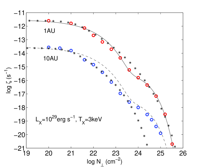
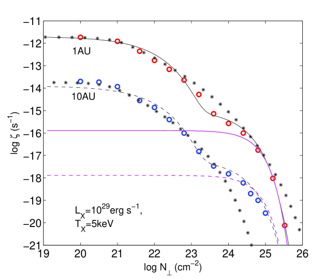
Figure 12: X-ray ionization rate as a function of disk column density, at 1 AU and 10 AU respectively. The central X-ray source is assumed to have X-ray luminosity $L_{X}=10^{29}$erg s^-1, and X-ray temperature $T_{X}=3$keV (upper panel) and $T_{X}=5$keV (bottom panel). Circles: values taken from Igea & Glassgold (1999). Asterisks: ionization rate with X-ray absorption only. Solid line: our fitted ionization rate for 1AU. Dashed line: rescaling of the fitted curve to 10AU. Pink curves are the fitting formula adopted by Turner & Sano (2008).

References

- Anders & Grevesse (1989) Anders, E. & Grevesse, N. 1989, Geochim. Cosmochim. Acta, 53, 197
- Balbus & Hawley (1991) Balbus, S. A. & Hawley, J. F. 1991, ApJ, 376, 214
- Balbus & Hawley (1998) —. 1998, Reviews of Modern Physics, 70, 1
- Barber et al. (2006) Barber, R. J., Tennyson, J., Harris, G. J., & Tolchenov, R. N. 2006, MNRAS, 368, 1087, (BT)
- Blaes & Balbus (1994) Blaes, O. M. & Balbus, S. A. 1994, ApJ, 421, 163
- Blandford & Payne (1982) Blandford, R. D. & Payne, D. G. 1982, MNRAS, 199, 883
- Carkner et al. (1996) Carkner, L., Feigelson, E. D., Koyama, K., Montmerle, T., & Reid, I. N. 1996, ApJ, 464, 286
- Carr & Najita (2008) Carr, J. S. & Najita, J. R. 2008, Science, 319, 1504
- Casanova et al. (1995) Casanova, S., Montmerle, T., Feigelson, E. D., & Andre, P. 1995, ApJ, 439, 752
- Cazaux & Tielens (2002) Cazaux, S. & Tielens, A. G. G. M. 2002, ApJ, 575, L29
- Cazaux & Tielens (2004) —. 2004, ApJ, 604, 222
- Chiang & Goldreich (1997) Chiang, E. I. & Goldreich, P. 1997, ApJ, 490, 368
- Chiang & Goldreich (1999) —. 1999, ApJ, 519, 279
- Chiang et al. (2001) Chiang, E. I., Joung, M. K., Creech-Eakman, M. J., Qi, C., Kessler, J. E., Blake, G. A., & van Dishoeck, E. F. 2001, ApJ, 547, 1077
- D’Alessio et al. (2006) D’Alessio, P., Calvet, N., Hartmann, L., Franco-Hernández, R., & Servín, H. 2006, ApJ, 638, 314
- D’Alessio et al. (1999) D’Alessio, P., Calvet, N., Hartmann, L., Lizano, S., & Cantó, J. 1999, ApJ, 527, 893
- Draine & Lee (1984) Draine, B. T. & Lee, H. M. 1984, ApJ, 285, 89
- Draine & Sutin (1987) Draine, B. T. & Sutin, B. 1987, ApJ, 320, 803
- Dullemond & Dominik (2005) Dullemond, C. P. & Dominik, C. 2005, A&A, 434, 971
- Freedman et al. (2008) Freedman, R. S., Marley, M. S., & Lodders, K. 2008, ApJS, 174, 504
- Fromang et al. (2002) Fromang, S., Terquem, C., & Balbus, S. A. 2002, MNRAS, 329, 18
- Gammie (1996) Gammie, C. F. 1996, ApJ, 457, 355
- Gammie & Balbus (1994) Gammie, C. F., & Balbus, S. A. 1994, MNRAS, 270, 138
- Giesen et al. (1992) Giesen, T., Schieder, R., Winnewisser, G., & Yamada, K. M. T. 1992, J. Mol. Spectrosc., 153, 406
- Glassgold et al. (1997) Glassgold, A. E., Najita, J., & Igea, J. 1997, ApJ, 480, 344
- Hartmann et al. (1998) Hartmann, L., Calvet, N., Gullbring, E., & D’Alessio, P. 1998, ApJ, 495, 385
- Hartmann et al. (2005) Hartmann, L., Megeath, S. T., Allen, L., Luhman, K., Calvet, N., D’Alessio, P., Franco-Hernandez, R., & Fazio, G. 2005, ApJ, 629, 881
- Hasegawa et al. (1992) Hasegawa, T. I., Herbst, E., & Leung, C. M. 1992, ApJS, 82, 167
- Hayashi (1981) Hayashi, C. 1981, Progress of Theoretical Physics Supplement, 70, 35
- Hayashi et al. (1985) Hayashi, C., Nakazawa, K., & Nakagawa, Y. 1985, in Protostars and Planets II, ed. D. C. Black & M. S. Matthews, 1100–1153
- Hollenbach & Salpeter (1970) Hollenbach, D. & Salpeter, E. E. 1970, J. Chem. Phys., 53, 79
- Ida & Lin (2008) Ida, S. & Lin, D. N. C. 2008, ApJ, 685, 584
- Igea & Glassgold (1999) Igea, J. & Glassgold, A. E. 1999, ApJ, 518, 848
- Ilgner & Nelson (2006a) Ilgner, M. & Nelson, R. P. 2006a, A&A, 445, 205, (IN06a)
- Ilgner & Nelson (2006b) —. 2006b, A&A, 445, 223
- Ilgner & Nelson (2008) —. 2008, A&A, 483, 815
- Jones et al. (1996) Jones, A. P., Tielens, A. G. G. M., & Hollenbach, D. J. 1996, ApJ, 469, 740
- Kim & Ostriker (2000) Kim, W.-T., & Ostriker, E. C. 2000, ApJ, 540, 372
- Krolik & Kallman (1983) Krolik, J. H. & Kallman, T. R. 1983, ApJ, 267, 610
- Mandell et al. (2008) Mandell, A. M., Mumma, M. J., Blake, G. A., Bonev, B. P., Villanueva, G. L., & Salyk, C. 2008, ApJ, 681, L25
- Mathis et al. (1977) Mathis, J. S., Rumpl, W., & Nordsieck, K. H. 1977, ApJ, 217, 425
- McCall et al. (2003) McCall, B. J., Huneycutt, A. J., Saykally, R. J., Geballe, T. R., Djuric, N., Dunn, G. H., Semaniak, J., Novotny, O., Al-Khalili, A., Ehlerding, A., Hellberg, F., Kalhori, S., Neau, A., Thomas, R., Österdahl, F., & Larsson, M. 2003, Nature, 422, 500
- Millar et al. (1997) Millar, T. J., Farquhar, P. R. A., & Willacy, K. 1997, A&AS, 121, 139
- Najita et al. (2003) Najita, J., Carr, J. S., & Mathieu, R. D. 2003, ApJ, 589, 931
- Natta et al. (2007) Natta, A., Testi, L., Calvet, N., Henning, T., Waters, R., & Wilner, D. 2007, in Protostars and Planets V, ed. B. Reipurth, D. Jewitt, & K. Keil, 767–781
- Nishi et al. (1991) Nishi, R., Nakano, T., & Umebayashi, T. 1991, ApJ, 368, 181
- O’Brien & Greenberg (2005) O’Brien, D. P. & Greenberg, R. 2005, Icarus, 178, 179
- Ogilvie & Livio (2001) Ogilvie, G. I. & Livio, M. 2001, ApJ, 553, 158
- Oishi et al. (2007) Oishi, J. S., Mac Low, M.-M., & Menou, K. 2007, ApJ, 670, 805
- Oppenheimer & Dalgarno (1974) Oppenheimer, M. & Dalgarno, A. 1974, ApJ, 192, 29
- Pessah et al. (2006) Pessah, M. E., Chan, C.-K., & Psaltis, D. 2006, MNRAS, 372, 183
- Press et al. (1992) Press, W. H., Teukolsky, S. A., Vetterling, W. T., & Flannery, B. P. 1992, Numerical recipes in C. The art of scientific computing (Cambridge: University Press, —c1992, 2nd ed.)
- Pringle (1981) Pringle, J. E. 1981, ARA&A, 19, 137
- Salmeron & Wardle (2008) Salmeron, R., & Wardle, M. 2008, MNRAS, 388, 1223
- Salyk et al. (2008) Salyk, C., Pontoppidan, K. M., Blake, G. A., Lahuis, F., van Dishoeck, E. F., & Evans, II, N. J. 2008, ApJ, 676, L49
- Sano et al. (2000) Sano, T., Miyama, S. M., Umebayashi, T., & Nakano, T. 2000, ApJ, 543, 486
- Sano & Stone (2002) Sano, T., & Stone, J. M. 2002, ApJ, 577, 534
- Semenov et al. (2004) Semenov, D., Wiebe, D., & Henning, T. 2004, A&A, 417, 93
- Sharp & Burrows (2007) Sharp, C. M. & Burrows, A. 2007, ApJS, 168, 140
- Shu (1991) Shu, F. H. 1991, in NATO ASIC Proc. 342: The Physics of Star Formation and Early Stellar Evolution, ed. C. J. Lada & N. D. Kylafis, 365–+
- Terquem (2008) Terquem, C. E. J. M. L. J. 2008, ApJ, 689, 532
- Townes & Schawlow (1955) Townes, C. H. & Schawlow, A. L. 1955, Microwave Spectroscopy (New York: McGraw-Hill)
- Turner & Sano (2008) Turner, N. J. & Sano, T. 2008, ApJ, 679, L131
- Turner et al. (2007) Turner, N. J., Sano, T., & Dziourkevitch, N. 2007, ApJ, 659, 729
- Umebayashi & Nakano (1981) Umebayashi, T. & Nakano, T. 1981, PASJ, 33, 617
- Umebayashi & Nakano (1990) —. 1990, MNRAS, 243, 103
- Vasyunin et al. (2008) Vasyunin, A. I., Semenov, D., Henning, T., Wakelam, V., Herbst, E., & Sobolev, A. M. 2008, ApJ, 672, 629
- Wardle (1999) Wardle, M. 1999, MNRAS, 307, 849
- Wardle (2007) —. 2007, Ap&SS, 311, 35
- Wardle & Koenigl (1993) Wardle, M. & Koenigl, A. 1993, ApJ, 410, 218
- Woodall et al. (2007) Woodall, J., Agúndez, M., Markwick-Kemper, A. J., & Millar, T. J. 2007, A&A, 466, 1197