Microwave response of superconducting pnictides: extended $s_{\pm}$ scenario

Abstract

We consider a two-band superconductor with relative phase $\pi$ between the two order parameters as a model for the superconducting state in ferropnictides. Within this model we calculate the microwave response and the NMR relaxation rate. The influence of intra- and interband impurity scattering beyond the Born and unitary limits is taken into account. We show that, depending on the scattering rate, various types of power law temperature dependencies of the magnetic field penetration depth and the NMR relaxation rate at low temperatures may take place.

1 Introduction

The recent discovery of Fe-based superconducting compounds [1] has stimulated the research of unconventional superconductors. One of the most important and still unsettled issues is the symmetry of the superconducting gap function. So far, different experiments produce conflicting results. As regards measurements of the penetration depth and the NMR relaxation rate, a power law behavior at low temperatures is now clearly established, which is a signature of unconventional order parameter symmetry. One possible scenario of a pairing symmetry state is a superconductor consisting of two relatively small semimetallic Fermi surfaces, separated by a finite wave vector $\mathbf{Q}$ with the relative phase $\pi$ between the two order parameters. This is the so-called $s_{\pm}$ model, first proposed in Ref. [2]. In our previous work [3] we have shown that $s_{\pm}$ model with strong impurity scattering can explain the power law behavior of the NMR relaxation rate. Therefore it is important to extend this formalism to address microwave properties of a two-band $s_{\pm}$ superconductor, in particular the magnetic field penetration depth and real part of complex conductivity, since experimental data are now available for single crystals of Fe-based superconductors.

In this paper we calculate the microwave response and the NMR relaxation rate for a model $s_{\pm}$ superconductor in which impurity scattering is treated beyond the Born limit and discuss the relevance to the experimental data for Fe-based superconducting compounds.

2 General expressions

We describe a multiband superconductor in the framework of the Eliashberg approach equations for the renormalization function $Z_{i}(\omega)$ and complex order parameter $\phi_{i}(\omega).$ As shown in the first reference of [21], the BCS approach can give highly inaccurate results in the case of interband superconductivity due to the BCS neglect of mass renormalization. In addition there is evidence for strong-coupling in the pnictides, with many experimentally determined $\Delta/T_{c}$ ratios substantially exceeding the BCS value of 1.76, and so we therefore employ the Eliashberg equations.

On the real frequency axis they have the following form, assuming an uniform ( band-independent) impurity scattering (see e.g., Ref.[3, 4, 5])

$$\phi_{i}(\omega) = \sum_{j}\int\limits_{-\infty}^{\infty}dzK_{ij}^{\Delta}(z,\omega)\mathrm{Re}g_{j}^{\Delta}(z)+\mathrm{i}\frac{\gamma}{2\mathcal{D}}\left(g_{1}^{\Delta}(\omega)-g_{2}^{\Delta}(\omega)\right)$$

$$(Z_{i}(\omega)-1)\omega = \sum_{j}\int\limits_{-\infty}^{\infty}dzK_{ij}^{Z}(z,\omega)\mathrm{Re}g_{j}^{Z}(z)+\mathrm{i}\frac{\gamma}{2\mathcal{D}}\left(g_{1}^{Z}(\omega)+g_{2}^{Z}(\omega)\right),$$ (1)

where $\mathcal{D}=1-\sigma+\sigma\left[\left(g_{1}^{Z}(\omega)+g_{2}^{Z}(\omega)\right)^{2}+\left(g_{1}^{\Delta}(\omega)-g_{2}^{\Delta}(\omega)\right)^{2}\right]$. For our model $g_{i}^{Z}(\omega)=n_{i}\left(\omega\right)Z_{i}(\omega)\omega/D_{i}(\omega)$, $g_{i}^{\Delta}(\omega)=n_{i}\left(\omega\right)\phi_{i}(\omega)/D_{i}(\omega)$, where $D_{j}(\omega)=\sqrt{\left[Z_{j}(\omega)\omega\right]^{2}-\phi_{j}^{2}(\omega)}$ and $n_{i}\left(\omega\right)$ is a partial density of states. $\gamma=2c\sigma/\pi N(0)$ is the normal-state scattering rate, N(0) is the total density of states (i.e.summed over both bands) at the Fermi level, c is the impurity concentration, and $\sigma=$ $\frac{\left[\pi N(0)v\right]^{2}}{1+\left[\pi N(0)v\right]^{2}}$ is the impurity strength ($\sigma\rightarrow 0$ corresponds to the Born limit, while $\sigma=1$ to the unitary one). The kernels $K_{ij}^{\Delta,Z}(z,\omega)$ describe the electron-boson interaction and have forms

$$K_{ij}^{\Delta,Z}(z,\omega)=\int\limits_{0}^{\infty}d\Omega\frac{\tilde{B}_{ij}(\Omega)}{2}\left[\frac{\tanh\frac{z}{2T}+\coth\frac{\Omega}{2T}}{z+\Omega-\omega-i\delta}-\left\{\Omega\rightarrow-\Omega\right\}\right],$$

where the spin-fluctuation coupling function is $\tilde{B}_{ij}(\Omega)=B_{ij}(\Omega)==\lambda_{ij}{\pi\omega\Omega_{sf}}/({\Omega_{sf}^{2}+\omega^{2}})$ for the equation for $\phi$, and $\left|B_{ij}(\Omega)\right|$ for the equation for $Z$. Here $\lambda_{ij}$ is the coupling constant pairing band $i$ with band $j$ and $\Omega_{SF}$ is the spin fluctuation frequency. Note that all retarded interactions enter the equations for the renormalization factor $Z$ with a positive sign.

We note that the implementation of the band-independent impurity scattering is contained in the second term on the right-hand side of Eq. 1, where the $\gamma$ is applied to both bands (albeit with a relative minus sign in the first equation due to the order parameter sign change between bands). We have chosen such a band-independent scattering for several reasons, including consistency with the previously published work and to avoid a proliferation of parameter choices. However, recent work of Senga and Kontani [6] suggests that this assumption is justified on an experimental basis. Their Fig. 4 shows that only $\gamma_{inter}/\gamma_{intra}$ between 0.9 and 1 is consistent with the several sets of nuclear spin relaxation rate T${}_{1}^{{}_{1}}$ data showing $T^{2.5}-T^{3.0}$ behavior over a very large temperature range. The theoretical rationale for such a comparatively large interband scattering rate remains unclear, but can be plausibly related to the inherent disorder in these systems, with the dopant atoms themselves acting as scattering centers.

The microwave conductivity in the London (local, $\mathbf{q}\equiv 0$) limit is given by

$$\sigma^{i}(\omega)=\omega_{pl,i}^{2}\Pi_{i}(\omega)/4\pi i\omega,$$ (2)

where $\Pi_{i}(\omega)$ is an analytical continuation to the real frequency axis of the polarization operator (see, e.g. Refs. [7],[8],[9],[10],[11])

$$\Pi_{i}(\omega)=\left\{i\pi T\sum_{n}\Pi_{i}(\omega_{n},\nu_{m})\right\}_{i\omega_{m}\Longrightarrow\omega+i0^{+}},$$

$$\Pi_{i}(\omega) = \int d\omega^{\prime}\left\{\frac{\tanh\left(\frac{\omega_{-}}{2T}\right)}{D^{R}}\right|\left[1-\frac{\tilde{\omega}_{-}^{R}\tilde{\omega}_{+}^{R}{\large+}\phi_{-}^{R}\phi_{+}^{R}}{\sqrt{(\tilde{\omega}_{\_}^{R})^{2}\mathbf{-(}\phi_{-}^{R})^{2}}\sqrt{(\tilde{\omega}_{+}^{R})^{2}\mathbf{-(}\phi_{+}^{R})^{2}}}\right]-$$

$$\frac{\tanh\left(\frac{\omega_{+}}{2T}\right)}{D^{A}}\left[1-\frac{\tilde{\omega}_{-}^{A}\tilde{\omega}_{+}^{A}\mathbf{+}\phi_{-}^{A}\phi_{+}^{A}}{\sqrt{(\tilde{\omega}_{\_}^{A})^{2}\mathbf{-(}\phi_{-}^{A})^{2}}\sqrt{(\tilde{\omega}_{+}^{A})^{2}\mathbf{-(}\phi_{+}^{A})^{2}}}\right]-$$

$$\frac{\tanh\left(\frac{\omega_{+}}{2T}\right)-\tanh\left(\frac{\omega_{-}}{2T}\right)}{D^{a}}\left|\left[1-\frac{\tilde{\omega}_{-}^{A}\tilde{\omega}_{+}^{R}\mathbf{+}\phi_{-}^{A}\phi_{+}^{R}}{\sqrt{(\tilde{\omega}_{\_}^{A})^{2}\mathbf{-(}\phi_{-}^{A})^{2}}\sqrt{(\tilde{\omega}^{R})^{2}\mathbf{-(}\phi_{+}^{R})^{2}}}\right]\right\},$$

where

$$D^{R,A}=\sqrt{(\tilde{\omega}_{+}^{R,A})^{2}\mathbf{-(}\phi_{+}^{R,A})^{2}}+\sqrt{(\tilde{\omega}_{\_}^{R,A})^{2}\mathbf{-(}\phi_{-}^{R,A})^{2}},$$

and

$$D^{a}=\sqrt{(\tilde{\omega}_{+}^{R})^{2}\mathbf{-(}\phi_{+}^{R})^{2}}-\sqrt{(\tilde{\omega}_{\_}^{A})^{2}\mathbf{-(}\phi_{-}^{A})^{2}},$$

$\omega_{\pm}=\omega^{\prime}\pm\omega/2$, and the index $R(A)$ corresponds to the retarded (advanced) brunch of the complex function $F^{R(A)}={Re}F\pm i{Im}F$ ( the band index $i$ is omitted), and $\tilde{\omega}=Z_{i}(\omega)\omega$. Here $\omega_{pl}^{\alpha\beta}=\sqrt{8\pi e^{2}\langle N_{i}(0)v_{F}^{\alpha}v_{F}^{\beta}\rangle}$ is the plasma frequency in different directions. For the dirty case the low frequency limits of expressions 2 and 2 can be reduced to the strong coupling generalization of the famous Mattis-Bardeen expressions [12]

$$\sigma_{1}(\omega \rightarrow 0)=\sigma_{1}^{\textrm{dc}}\int\limits_{0}^{\infty}d\omega\left(-\frac{\partial f(\omega)}{\partial\omega}\right)\left\{\left[\mathrm{Re}g_{1}^{Z}(\omega)\right]^{2}+\left[\mathrm{Re}g_{1}^{\Delta}(\omega)\right]^{2}\right\}+$$ (4)

$$\sigma_{2}^{\textrm{dc}}\int\limits_{0}^{\infty}d\omega\left(-\frac{\partial f(\omega)}{\partial\omega}\right)\left\{\left[\mathrm{Re}g_{2}^{Z}(\omega)\right]^{2}+\left[\mathrm{Re}g_{2}^{\Delta}(\omega)\right]^{2}\right\},$$

where $\sigma_{i}^{\textrm{dc}}=N_{i}(0)v_{F}^{2}e^{2}\tau_{i}$ is a contribution to the static conductivity from $i-$th band. Note that in the London limit there are no cross-terms connected two bands.

An important characteristic of the superconducting state is the penetration depth of the magnetic field $\lambda_{L,\alpha\beta}$ in the local (London) limit, which is related to the imaginary part of the optical conductivity by

$$1/\lambda_{L,\alpha\beta}^{2}=\lim_{\omega->0}4\pi\omega\mathop{\rm Im}\sigma^{\alpha\beta}(\omega,\mathbf{q}=0)/c^{2}\equiv\omega_{pl,i}^{\alpha\beta 2}{Re}\Pi_{i}(\omega=0)/c^{2},$$ (5)

where $\alpha,\beta$ denote again Cartesian coordinates and $c$ is the velocity of light. If we neglect strong-coupling effects (or, more generally, Fermi-liquid effects) then for a clean uniform superconductor at $T=0$ we have the relation $\lambda_{L,\alpha\beta}=c/\omega_{pl}^{\alpha\beta}$. Impurities and interaction effects drastically enhance the penetration depth, and it is suitable to introduce a so called ’superfluid plasma frequency’ $\omega_{pl,\alpha\beta}^{sf}$ by the relation $\omega_{pl,\alpha\beta}^{sf}=c/\lambda_{L,\alpha\beta}$. It has been often mentioned that this function corresponds to the charge density of the superfluid condensate, but we would like to point out that this is only the case for noninteracting clean systems at $T=0$.

In the two-band model we have the standard expression (neglecting vertex corrections)

$$1/\lambda_{L,\alpha\beta}^{2}(T) \equiv (\omega_{pl,\alpha\beta}^{sf}(T)/c)^{2}=$$

$$\sum_{i}\left(\frac{\omega_{pl,i}^{\alpha\beta}}{c}\right)^{2}\pi T\sum_{n=-\infty}^{\infty}\frac{\tilde{\Delta}_{i}^{2}(n)}{[\tilde{\omega}_{i}^{2}(n)+\tilde{\Delta}_{i}^{2}(n)]^{3/2}},$$

where $\tilde{\omega}(n)$ and $\tilde{\Delta}(n)$ are the solutions of Eq. 1 continued to the imaginary (Matsubara) frequencies ($\tilde{\Delta}_{i}(n)=\phi_{i}(i\omega_{n}),$ $\tilde{\omega}_{i}(n)=\omega_{n}Z_{i}(i\omega_{n})$). The calculations along these formulas can be thus presented in form of the effective superfluid plasma frequency, $\omega_{pl}^{sf}.$

For the NMR relaxation rate, following [13], we can write down the following general expressions.

$$1/T_{1}T=-\frac{1}{2\pi}\lim_{\omega\rightarrow 0}\sum_{\mathbf{q}}\left[F(\mathbf{q})\right]^{2}\frac{{Im}\chi_{\pm}(\mathbf{q},\omega)}{\omega},$$ (7)

where $\chi_{\pm}(\mathbf{q},\omega)$ is an analytical continuation to the real axis of the Fourier  transform of the correlator

$$\chi_{\pm}(\mathbf{r},\tau)=-\left\langle\left\langle T_{\tau}(S_{+}(\mathbf{r},-i\tau)S_{-}(\mathbf{0},0)\right\rangle\right\rangle_{imp}.$$

averaged over the impurity ensemble. Here $S_{\pm}(\mathbf{r},-i\tau)=\exp(H\tau)S_{\pm}(\mathbf{r})\exp(-H\tau)$ where $H$ is the electron Hamiltonian, $\tau$ denotes imaginary time, and $S_{+}(\mathbf{r})=\psi_{\uparrow}^{{\dagger}}(\mathbf{r})\psi_{\downarrow}(\mathbf{r})$ and $S_{-}(\mathbf{r})=\psi_{\downarrow}^{{\dagger}}(\mathbf{r})\psi_{\uparrow}(\mathbf{r}).$ As a result we have

$$1/T_{1}T = \frac{1}{\pi^{2}}\sum_{\mathbf{k}_{1},\mathbf{k}_{2}}\int_{-\infty}^{\infty}d\omega(-\frac{\partial f(\omega)}{\partial\omega})\sum_{i,j}\left[F_{ij}(\mathbf{k}_{1}-\mathbf{k}_{2})\right]^{2}\times$$

$$\left[{Im}\frac{\omega Z_{i,\mathbf{k}_{1}}(\omega)}{D_{i,\mathbf{k}_{1}}(\omega)}{Im}\frac{\omega Z_{j,\mathbf{k}_{2}}(\omega)}{D_{j,\mathbf{k}_{2}}(\omega)}\right.+$$

$${Im}\frac{\xi_{i,\mathbf{k}_{1}}}{D_{i,\mathbf{k}_{1}}(\omega)}{Im}\frac{\xi_{j,\mathbf{k}_{2}}}{D_{j,\mathbf{k}_{2}}(\omega)}+$$

$$\left.{Im}\frac{\phi_{i,\mathbf{k}_{1}}(\omega)}{D_{i,\mathbf{k}_{1}}(\omega)}{Im}\frac{\phi_{j,\mathbf{k}_{2}}(\omega)}{D_{j,\mathbf{k}_{2}}(\omega)}\right].$$

Here $D_{i,\mathbf{k}_{1}}(\omega)=\left[\omega Z_{i,\mathbf{k}_{1}}(\omega)\right]^{2}-\xi_{i,\mathbf{k}_{1}}^{2}-\phi_{i,\mathbf{k}_{1}}^{2}(\omega)$, $\xi_{i,\mathbf{k}_{1}}$is the bare energy. For the Fermi-contact interaction

$$\frac{1}{T_{1}T}\propto\int\limits_{0}^{\infty}d\omega\left(-\frac{\partial f(\omega)}{\partial\omega}\right)\left\{\left[\mathrm{Re}g_{1}^{Z}(\omega)+\mathrm{Re}g_{2}^{Z}(\omega)\right]^{2}+\left[\mathrm{Re}g_{1}^{\Delta}(\omega)+\mathrm{Re}g_{2}^{\Delta}(\omega)\right]^{2}\right\}.$$ (9)

This expression contains the cross-term in contrast to the microwave conductivity. In this paper, in the T${}_{1}^{{}_{1}}$ calculation only these cross terms are used to emphasize the interband character of the superconductivity, as it is these cross terms that are most enhanced by the nearly antiferromagnetic state within a more detailed RPA approximation. For a single band system the full expression is proportional to Eq.4 when $\sigma_{1}^{\textrm{dc}}\rightarrow\infty$ (Ref. [14]), but in multiband systems $1/T_{1}T$ and $\sigma_{1}(\omega\rightarrow 0)$ can behave differently.

3 Results and discussion

It is well known that pair-breaking impurity scattering can induce substantial sub-gap density of states, which can produce power-law low temperature behavior in a whole host of thermodynamic quantities, such as specific heat, London penetration depth, nuclear spin relaxation rate, and even optical conductivity. Such behavior has been well-studied in the two canonical limits of weak (Born) scattering and strong (unitary) scattering [15] , but the intermediate regime has received almost no attention. In addition, with the advent of the multiband superconductivity in MgB₂ and the apparent multiband, primarily interband superconductivity in the pnictides, comes a need for further study of the intermediate regime in an interband case. Recent studies [16, 19, 17] have addressed the effects of impurities in the pnictides, but only in the Born or unitary limits. Here we study the important and likely more realistic intermediate regime, with $\sigma$, effectively the scattering strength is varied in the range from $\sigma=0$ corresponding to the Born limit to $\sigma=1$ corresponding to the unitary limit. As stated earlier, for all calculations the impurity scattering rate $\gamma_{intra}=\gamma_{inter}=0.8\Delta_{0}$.

We will now illustrate the above discussion using specific numerical models. First, we present numerical solutions of the Eliashberg equations using the spin-fluctuation model for the spectral function of the intermediate boson: $B_{ij}(\omega)=\lambda_{ij}{\pi\omega\Omega_{sf}}/({\Omega_{sf}^{2}+\omega^{2}})$, with the parameters $\Omega_{sf}=25$meV, $\lambda_{11}=\lambda_{22}=0.5$, and $\lambda_{12}=\lambda_{21}=-2$. The rather large coupling constants are an attempt to model the rather large experimentally observed ratio $\Delta/T_{c}$. This set gives a reasonable value for $T_{c}\simeq 26.7$K. A similar model was used in Ref. [20] to describe optical properties of ferropnictides. This model was also

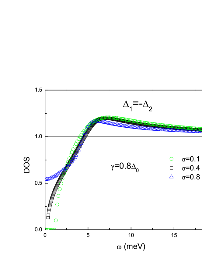
Figure 1: (color online) The quasiparticle density of states for the three indicated cases. The near-Born case $\sigma=0.1$ retains a small gap, while the intermediate case shows a monotonic DOS and the near-unitary is gapless.

used in [3] and for consistency is used here. As stated earlier, we further assume that each surface features the same gap [21], and that the intraband impurity scattering rate and interband scattering rate are both equal to $0.8\Delta_{0}$, where $\Delta_{0}$ is the low-temperature limiting value of the superconducting gap $\Delta$.As in [3], we have chosen a relatively large impurity scattering, which is to be expected considering the early state of pnictide sample preparation and the limited availability of large single crystals.

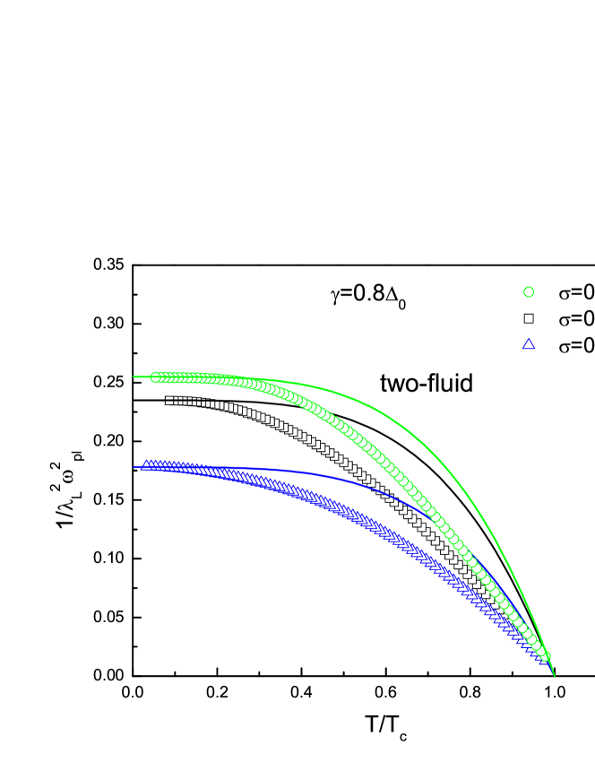
Figure 2: (color online) The inverse squared penetration depth. The near-Born limit approaches the BCS ”two-fluid” calculation ($\propto 1-T^{4}$) at low temperatures, mimicking exponential behavior, while the other two cases show power-law behavior, as in Fig. 3.

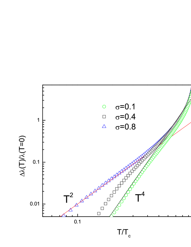
Figure 3: (color online) The low temperature behavior of the penetration depth, showing the evolution with decreasing $\sigma$ from T² gapless behavior towards the exponential-mimicking T⁴ character.

We begin with the density of states, shown below in Figure 1. Several effects are apparent. Firstly, for all three $\sigma$ values the substantial peak usually present at $\omega=\Delta_{0}$ (about 6 meV here) is substantially truncated, with much spectral weight transferred below the gap. However, the detailed sub-gap behavior depends radically upon the scattering strength $\sigma$. The near-Born case $\sigma=0.1$ still retains a small minigap of approximately 1.5 meV, which will lead to exponentially activated behavior below about 4 Kelvin. Although some data has shown evidence for such exponentially activated behavior, there is also significant data showing power-law behavior. The intermediate case $\sigma=0.4$ shows a monotonically increasing density of states and essentially no minigap, leading to power-law behavior, as proposed in [3]. Finally, the near-unitary case $\sigma=0.8$ also shows a monotonically increasing density of states, but is nearly constant at low energy. We will see that such behavior leads to a quadratic temperature dependence of the penetration depth, even without the assumption of the strict unitary limit. Gross et. al. some time ago noted [18] in a different context that T² behavior does not require the unitary limit. We note parenthetically that the behavior depicted depends rather strongly upon the large value of impurity scattering assumed; the first two cases will yield more exponentially activated behavior if the scattering rate is much less strong, while the near-unitary case can potentially [4] lead to a non-monotonic density of states.

In Figure 2 is shown the inverted squared London penetration depth $1/\lambda^{2}(T)$, the so-called superfluid density for several cases as indicated in the figure. In all cases the temperature dependence of $1/\lambda^{2}(T)$ is different from the standard two-fluid (Gorter-Casimir) model $\lambda^{-2}(T)=\lambda^{-2}(0)\left[1-\left(T/T_{c}\right)^{4}\right]$, that is similar to the BCS result. Due to the sign change between gaps, the interband component of the scattering matrix is strongly pair-breaking, analogously to magnetic scattering in s-wave superconductors. As a result, the superfluid density shows near-exponential character at low temperature in the near-Born case ($\sigma=0.1$), while the other two cases ($\sigma=0.4$ and $0.8$) exhibit power-law behavior at low T, with the actual power varying between 2 and 3.

A more detailed view of the low-temperature $\lambda(T)$ power law behavior is presented in Figure 3, which shows $\Delta\lambda(T)/\lambda_{T=0}$ for the same three cases. We see that the near-Born limit case ($\sigma=0.1$) approaches a T⁴ behavior, reminiscent of a two fluid model, while the near-unitary case shows a fairly robust T² behavior and the intermediate case falls between these two limits, as one would naively expect. Experimental data available so far [23, 24, 25] are consistent with either T² , or T⁴ or exponential (gapped) behavior. Within our model, both results can be explained by proper choice of the impurity scattering rate. It is interesting to note that the $T^{2}$ dependence we obtain corresponds to strongly gapless regime. Similar results were obtained recently in Ref.[19] but in the Born limit only.

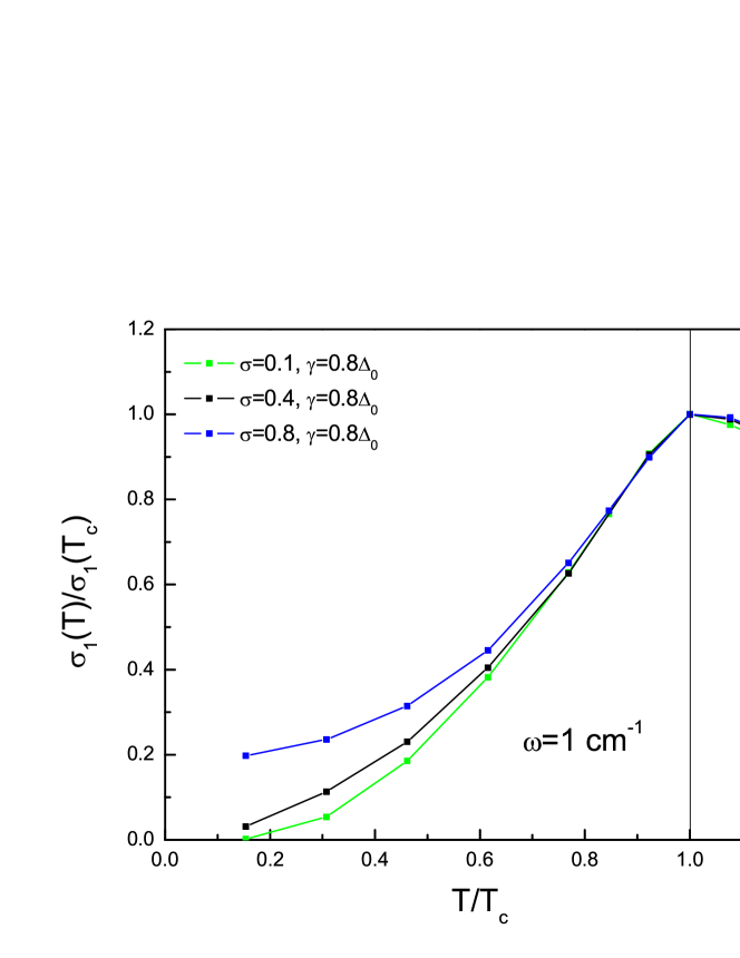
Figure 4: (color online) The real part of the microwave conductivity. Note the substantial increase with scattering strength at low temperature.

Figure 4 shows the calculated real part of the microwave conductivity for the three cases above. The microwave conductivity( Fig. 4) $\sigma_{1}(T)$ does not show the coherence peak near $T_{c}$. The suppression is connected with strong-coupling effects (see, [22]). Below $T_{c}$ the behavior of the $\sigma_{1}(T)$ is determined by the filling of the impurity induced states below $\Delta.$ Qualitatively it is similar to the temperature dependence of the NMR relaxation rate ( see Fig. 5), but in the latter case the Hebel-Slichter peak is additionally reduced for $s_{\pm}$ model by the different kind of the coherence factor. Almost all of the non-canonical BCS behavior derives from the interband component of the scattering matrix, which results in near constant behavior at low T for the near-unitary case, as might be expected from the form of Equation 4, in which a squared density of states enters. The intermediate case shows power law behavior as well, with the precise exponent not extracted.

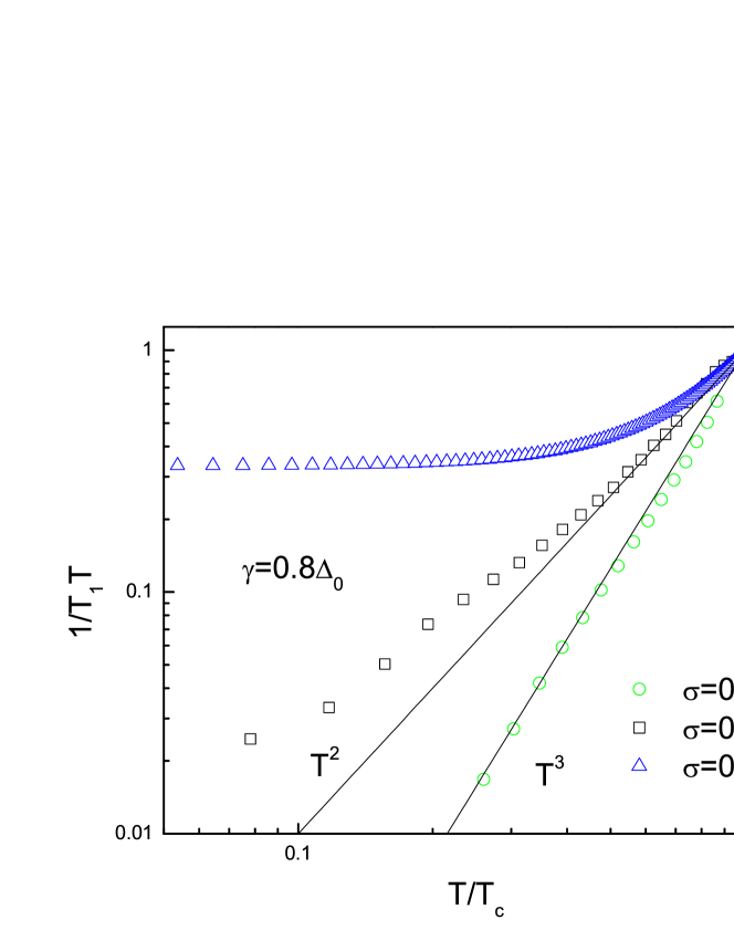
Figure 5: (color online) The temperature dependence of the relaxation rate $1/T_{1}T$, exhibiting near-Korringa behavior for $\sigma=0.8$ and power-law behavior for the other curves.

Finally we turn in Figure 5 to the nuclear spin relaxation rate $T_{1}^{-1}$ for the same three $\sigma$ scenarios. Note also that following convention we have plotted $(T_{1}T)^{-1}$ rather than T${}^{-1}_{1}$, and all power-law references here mean $(TT_{1})^{-1}$. T₁ has been a source of substantial controversy in the pnictides due to the existence of several data-sets [26, 27, 28, 29] showing near-T² behavior throughout nearly the entire temperature range, although there now exist data [30] deviating from this behavior. Several things are apparent from the plot: first of all, the near-Born limit case shows power law behavior ($1/T_{1}T\sim T^{3}$) throughout nearly the entire temperature range below T_c, although it will ultimately revert to exponentially activated behavior at the lowest temperatures. Substantial impurity scattering in the Born limit can thus mimic much of the behavior commonly ascribed to nodes, as was noted in [17, 19]. The intermediate case shows an approximate T^1.5 behavior, as was described in [3], which is largely driven by the monotonic density of states presented in Figure 1, where the same parameters are chosen. Korringa behavior results in the near-unitary limit, as is again a direct consequence of the corresponding behavior of the density of states in Figure 1, but does not result in either of the first two cases unless the scattering rate $\gamma$ is increased significantly beyond $0.8\Delta_{0}$.

It should now be clear that impurity scattering in various strengths (i.e, $\sigma$), if sufficient impurity concentrations are present, can produce a wide variety of power-law behaviors in many thermodynamic quantities, even in the near-Born limit. In the s_± state, interband impurities are clearly much more effective in creating such behavior. This has implications for the ongoing lively debate about pairing symmetry, with significant numbers of proposals for nodal superconductivity in the pnictides and some experimental evidence for such behavior.

In conclusion, we have calculated the microwave response and the NMR relaxation rate for a superconductor in $s_{\pm}$ symmetry state by solving Eliashberg equations with a model spectrum and taking into account impurity scattering beyond the Born limit. We show that the $T^{2}$ temperature behavior of the penetration depth and the NMR relaxation rate at low temperatures can be reproduced in this model. We have also demonstrated the dramatic effect of the impurity scattering on the real part of the microwave conductivity, which in particular results in near constant behavior at low T for the near-unitary case.

References

- [1] Y. Kamihara et al., J. Am. Chem. Soc. 130, 3296 (2008).
- [2] I.I. Mazin, D.J. Singh, M.D. Johannes, and M.H. Du, Phys. Rev. Lett, 101, 057003 (2008).
- [3] D. Parker, O. V. Dolgov, M. M. Korshunov, A.A. Golubov and I.I. Mazin, Phys. Rev. B 78, 134524 (2008).
- [4] G. Preosti and P. Muzikar, Phys. Rev. B 54, 3489 (1996).
- [5] A.A. Golubov and I.I. Mazin, Phys. Rev. B 55, 15146 (1997).
- [6] Y. Senga and H. Kontani, New J. Phys. 11, 035005 (2009).
- [7] S.B. Nam, Phys. Rev., 156, 470 (1967).
- [8] W. Lee, D.Rainer, and W. Zimmermann, Physica C 159, 535 (1988).
- [9] O.V. Dolgov, A.A. Golubov, and S.V. Shulga, Phys. Letters A 147, 317 (1990).
- [10] R. Akis and J.P. Carbotte, Solid State Comm., 79, 577 (1991).
- [11] F. Marsiglio, Phys. Rev. B 44, 5373 (1991).
- [12] D.C. Mattis and J. Bardeen, Phys. Rev. 111, 412 (1958).
- [13] D.D. MacLaughlin in Solid State Physics, edited by H. Ehrenreich, F. Seitz and D. Turnbull, Vol. 31, p.34 (1976).
- [14] F. Marsiglio, J.P. Carbotte, R. Akis, D. Achkir, and M. Poirier, Phys Rev. B 50, 7203(R), (1994).
- [15] P.J. Hirschfeld, P. Wölfle, and D. Enzel, Phys. Rev. B 37, 83 (1988); A.E. Karakozov, E.G. Maksimov, and A.V. Andrianova, JETP Letters, 79, 329 (2004).
- [16] Y. Bang, arXiv:0902.1020 (unpublished).
- [17] A.V. Chubukov, D. V. Efremov, and I. Eremin, Phys. Rev. B 78, 134512 (2008).
- [18] F. Gross, B. S. Chandrasekhar, D. Einzel, K. Andres, P. J. Hirschfeld, H. R. Ott, J. Beuers, Z. Fisk and J. L. Smith, Z. Phys. B 64, 175 (1986).
- [19] A.V. Vorontsov, M.G. Vavilov, A.V. Chubukov, arXiv:0901.0719 (unpublished).
- [20] J. Yang, D. Huvonen, U. Nagel, T. Room, N. Ni, P.C. Canfield, S.L. Budko, J.P. Carbotte, and T. Timusk, arXiv:0807.1040 (unpublished).
- [21] In the weak coupling limit, the gap ratio at in the model is , where are densities of states. LDA calculations yield , therefore and differ by less than 10%. Strong coupling effects additionaly reduce the gaps ratio (see, O.V. Dolgov, I.I. Mazin, D. Parker, and A.A. Golubov, Phys. Rev. B 79, 060502(R) (2009); O.V. Dolgov and A.A. Golubov, Phys. Rev. B 77, 214526 (2008)).
- [22] O.V. Dolgov, A.A. Golubov, and A.E. Koshelev, Solid State Comm. 72, 81 (1989); P.B. Allen and D. Rainer, Nature 439, 396 (1991).
- [23] C. Martin, M. E. Tillman, H. Kim, M. A. Tanatar, S. K. Kim, A. Kreyssig, R. T. Gordon, M. D. Vannette, S. Nandi, V. G. Kogan, S. L. Bud’ko, P. C. Canfield, A. I. Goldman, and R. Prozorov, arXiv:0903.2220 (unpublished); C. Martin, R.T. Gordon, M. A. Tanatar, H. Kim, N. Ni, S. L. Bud’ko, P. C. Canfield, H. Luo, H. H. Wen, Z. Wang, A. B. Vorontsov, V. G. Kogan, and R. Prozorov, arXiv:0902.1804 (unpublished); R. T. Gordon, C. Martin, H. Kim, N. Ni, M. A. Tanatar, J. Schmalian, I. I. Mazin, S. L. Bud’ko, P. C. Canfield, and R. Prozorov, arXiv:0812.3683 (unpublished).
- [24] L. Malone, J.D. Fletcher, A. Serafin, A. Carrington, N.D. Zhigadlo, Z. Bukowski, S. Katrych, and J. Karpinski, arXiv:0806.3908 (unpublished).
- [25] K. Hashimoto, T. Shibauchi, S. Kasahara, K. Ikada, T. Kato, R. Okazaki, C. J. van der Beek, M. Konczykowski, H. Takeya, K. Hirata, T. Terashima, and Y. Matsuda, arXiv:0810.3506 (unpublished); K. Hashimoto, T. Shibauchi, T. Kato, K. Ikada, R. Okazaki, H. Shishido, M. Ishikado, H. Kito, A. Iyo, H. Eisaki, S. Shamoto, and Y. Matsuda, Phys. Rev. Lett. 102, 017002 (2009).
- [26] H.-J. Grafe,D. Paar, G. Lang, N.J. Curro, G. Behr, J. Werner, J. Hamann-Borrero, C. Hess, N. Leps, R. Klingeler, and B. Büchner, Phys. Rev. Lett. 101, 047003 (2008).
- [27] Y. Nakai, K. Ishida, Y. Kamihara, M. Hirano, and H. Hosono, Phys. Rev. Lett. 101, 077006 (2008).
- [28] K. Matano, Z.A. Ren, X.L. Dong, L.L Sun, Z.X. Ghao, and G.-Q. Zheng, Europhys. Lett. 83, 57001 (2008).
- [29] H. Mukuda N. Terasaki, H. Kinouchi, M. Yashima, Y. Kitaoka, S. Suzuki, S. Miyasaka, S. Tajima, K. Miyazawa, P.M. Shirage, H. Kito, H. Eisaki, and A. Iyo, J. Phys. Soc. Jpn. 77, 093704 (2008); H. Kotegawa, S. Masaki, Y. Awai, H. Tou, Y. Mizuguchi and Y. Takano, J. Phys. Soc. Jpn. 77, 113703 (2008).
- [30] Y. Kobayashi, A. Kawabata, S.C. Lee, T. Moyoshi and M. Sato, arXiv:0901.2830 (unpublished); H. Fukazawa, T. Yamazaki, K. Kondo, Y. Kohori, N. Takeshita, P.M. Shirage, K. Kihou, K. Miyazawa, H. Kito , H. Eisaki, and A. Iyo, arXiv:0901.0177 (unpublished); K. Tatsumi, N. Fujiwara, H. Okada, H. Takahashi, Y. Kamihara, M. Hirano, and H. Hosono, Journal of Phys. Soc. Jpn., 78, 023709 (2009).