Quantum states prepared by realistic entanglement swapping

Abstract

Entanglement swapping between photon pairs is a fundamental building block in schemes using quantum relays or quantum repeaters to overcome the range limits of long distance quantum key distribution. We develop a closed-form solution for the actual quantum states prepared by realistic entanglement swapping, which takes into account experimental deficiencies due to inefficient detectors, detector dark counts and multi-photon-pair contributions of parametric down conversion sources. We investigate how the entanglement present in the final state of the remaining modes is affected by the real-world imperfections. To test the predictions of our theory, comparison with previously published experimental entanglement swapping is provided.

PACS numbers: 03.67.-a, 03.67.Bg, 03.67.Dd, 03.67.Hk, 42.50.Ex

I Introduction

Quantum cryptographic communication and quantum key distribution technologies have matured to a level sufficient for commercial applications. Yet, distance limits impact on their usefulness. To date, the only realistic proposals for long distance quantum cryptography are still based on optical systems. Light is an optimal candidate to be a carrier of quantum information because photonic quantum states are durable due to their generally weak interaction with the environment and are conveniently manipulated by means of linear optics and photon-detection. Moreover, photons are the fastest and one of the simplest physical systems for encoding quantum information. The technological challenge is to establish transmission channels over long distances with a high signal-to-noise ratio using real-world optical fiber settings or free space. Long distance quantum communication (LDQC) is hampered by a significant loss of photons with distance traveled. In particular, loss of photons due to absorption during transmission in fibers is characterized by the exponential rule $t=10^{-\alpha d/10}\;,$ where $t$ is the transmission coefficient, $d$ is the distance traveled and $\alpha$ is the loss coefficient of the transmission medium in units of dB. A further limitation to the development of quantum communication over long distances is a constant detector noise level dominating over the exponential decrease of the signal. In an effort to overcome these obstacles and range limits of LDQC, quantum repeaters BriegelDuerCiracZoller1998 ; Duan2001 or quantum relays Gisin2002 ; Waks2002 ; Jacobs2002 ; Riedmatten2004 ; Collins2005 have been proposed, which comprise entanglement swapping Zukowski1993 as a fundamental building block.

In principle, quantum repeaters enable any distance to be achieved. The basic idea of a quantum repeater is to split the long distance quantum channel into shorter segments and to distribute entanglement between the end nodes of these segments. Then, after purifying the noisy entanglement for each segment, the entanglement is extended over adjacent segments by means of entanglement swapping. The purification procedure is repeated for the extended segments, and the whole protocol reiterated until high-purity entanglement is established between the end points of the channel. A quantum relay works in a similar way as the quantum repeater, but without the entanglement purification procedure and without quantum memories. This makes it much more feasible as compared to the repeater, but does not allow achieving arbitrary distances Collins2005 . With both schemes the signal-to-noise ratio can be appreciably increased. However, experimental realization Collins2005 suffers from a number of imperfections, including imperfect sources of entangled pairs and imperfect detectors.

The impact of experimental deficiencies on the security of a quantum channel as well as on sifted and secret key rates in quantum key distribution (QKD) is of considerable relevance and has been the objective of a number of recent investigations. In Brassard2000 Brassard et al. showed that channel losses, a realistic detection process comprising detector inefficiencies and dark counts, and imperfections in the qubit source drastically impair the feasibility of QKD over long distances. In particular, the implications of using attenuated laser pulses instead of idealized single-photon on-demand sources were examined, and it was shown that unconditional security is very difficult to achieve in long distance QKD based on a BB84 protocol BB84 with such weak laser pulses. In the same work Brassard and coworkers obtained a more optimistic performance for QKD schemes based on parametric down-conversion (PDC) sources Ekert92 ; Sergienko99 . The consequences of using probabilistic photon-pair sources (as realized by PDC) instead of (non-existing) single-pair on-demand sources for quantum communication including entanglement based QKD have recently further been investigated, see Ma2007 ; Marcikic2002 ; Riedmatten2003 .

For LDQC employing quantum repeaters or relays it is particularly important to examine the issue of how the entangled quantum states after an entanglement swapping operation are affected by experimental imperfections. It is clear that due to these imperfections the actual quantum states deviate from desired Bell states and have to be described by some mixed states. The impact of transmission losses and detector inefficiencies as well as dark counts on the performance of quantum relays has been recently examined by Collins et. al. in Collins2005 . However, the probabilistic nature of photon-pair sources has not been considered in their work. As will be explained in the next section, the probabilistic nature of PDC also involves the possibility of multi-pair generation. Depending on the “brightness” of the sources, the emission of two (or even more) independent pairs of entangled photons from the same PDC source at a time becomes a more or less significant event leading to faulty detection clicks and incorrect conclusions with regard to entanglement and correlations. Thus, the multi-pair nature of PDC sources impairs a high fidelity realization of entanglement swapping. The investigation of the issue as to what extent the inevitable multi-pair contributions of PDC sources impinge on the performance of quantum communication protocols based on entanglement swapping, is the main motivation for the research presented in this article. The effect of multi-excitation events in PDC in addition to detector imperfections and transmission losses on quantum repeater performance has been examined perturbatively in the context of single-rail entanglement by Brask and Sørensen in BraskSorensen2008 . Furthermore, the atom-light entangled states produced by Stokes scattering in the DLCZ-scheme Duan2001 are very similar to the light-light entangled states produced in a non-degenerate PDC process, as both are two-mode squeezed states. In works by Jiang et al.  JiangTaylorLukin2007 and Zhao et al.  Zhao-et-al2007 , which extend the original DLCZ scheme to dual-rail entanglement, the consequence of multi-excitation events has also been treated in a perturbative way. In our work we choose a different approach, which is non-perturbative and essentially simpler, as it uses only the very basic toolbox of quantum theory and the principle of Bayesian inference.

In this article, we elaborate on how the entangled quantum states after entanglement swapping are affected by experimental imperfections, particularly the multi-pair contributions of PDC sources. We provide a non-perturbative theory for realistic entanglement swapping with imperfect photon-pair sources as well as imperfect detectors. In particular, we incorporate the multi-pair nature of PDC, transmission losses, and detector inefficiencies and dark counts non-perturbatively. Our theory enables us to obtain a closed-form analytic solution for the resultant mixed entangled quantum states after a real-world (noisy) entanglement swapping operation. To test our theory, we compare its predictions with actual experiments on entanglement swapping, that have been previously published elsewhere. For this purpose, we derive a closed-form expression for the probability of four-fold coincidences of four detectors, two for the Bell-state measurement and two for monitoring the remaining two entangled modes, one on each side, depending on variable polarization directions of analyzers. This result allows us to calculate numerically the visibility of four-fold coincidences for arbitrary parameter values characterizing real-world imperfections of the PDC sources and detectors. Finally, we inspect how the entanglement present in the final state of the remaining modes is affected by the practical deficiencies. The analysis makes it possible to suggest the implications of the imperfections on schemes using entanglement swapping as a fundamental tool, and to optimize parameter settings for maximum performance.

In addition to the imperfections of sources and detectors, further problems are encountered in a realistic entanglement swapping process. Imperfections of temporal overlap of the light fields on a beamsplitter as well as spectral mode mismatch constitute inevitable practical difficulties deteriorating the performance. Moreover, the entangled photon pairs prepared by two sources are expected not to be of the same quality. All of these problems would complicate the analysis and are not taken into account in the present study, but are planned to be included in our future work. Here, we would like to focus on implications of imperfect sources and imperfect detectors only. In this way, our considerations provide a very useful upper bound on the amount of entanglement after swapping. As for the influence of mode mismatch on the performance, we would like to refer the reader to models developed in Oezdemir2002 ; Rohde2006 ; Jia2005 .

Our work extends the previous challenge Brassard2000 to the security of QKD protocols using imperfect sources as well as the investigations in Collins2005 ; BraskSorensen2008 ; JiangTaylorLukin2007 ; Zhao-et-al2007 . Efforts toward establishing reliable transmission of quantum systems over arbitrary distances will benefit from our careful analysis presented here.

This article is organized as follows. In section II we develop our theory of real-world entanglement swapping. A mathematical description of imperfect photon-pair sources and imperfect detectors is provided. Using these models we derive a closed-form solution for the quantum states after a realistic entanglement swapping operation. In section III we apply our theory to making predictions with regard to entanglement verification in terms of the visibility of four-fold coincidences and compare our numerical results with experimental entanglement swapping. We proceed with a discussion of the impact of experimental deficiencies on the entanglement of the resultant quantum state. We conclude with a brief summary and suggestions for future research in section IV.

II A theory for practical entanglement swapping

II.1 Physical situation and setting

In this paper we develop our theory for entanglement swapping of photon-polarization qubits as an illustrative example. However, the main issues of the theory apply to any other photonic realization of qubits TittelWeihs2001 and the results and implications are independent of the latter. The basic experimental situation is illustrated in Fig. 1. Two parametric down conversion sources emit photon pairs into spatial modes $a$, $b$, $c$ and $d$, where $a$ and $b$ correspond to the first and $c$ and $d$ to the second PDC source. In the ideal-case scenario, one entangled photon-pair is emitted into the $a$ and $b$ modes and another one into the $c$ and $d$ modes. For entanglement swapping, a joined Bell-state measurement is performed on the $b$ and $c$ modes. This results in projecting the remaining modes $a$ and $d$ onto an entangled state, depending on the measurement readout of the Bell-state measurement. As a consequence, the photons in the outgoing $a$ and $d$ modes emerge entangled despite never having had an interaction with one another Zukowski1993 . The entanglement previously contained in the $a$ and $b$ and the $c$ and $d$ photon pairs is swapped to the $a$ and $d$ photon pair.

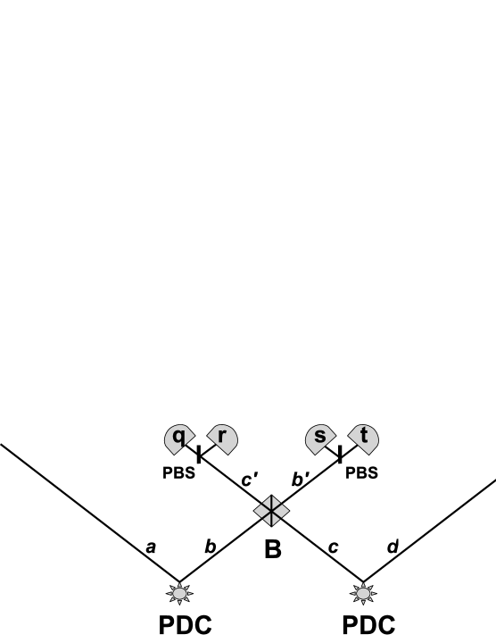
Figure 1: Entanglement swapping of photon-polarization qubits, based on two imperfect parametric down conversion sources (PDC) and a Bell-measurement with four imperfect photon detectors. Four spatial modes are involved, labeled by $a$, $b$, $c$ and $d$. Two modes, one from the first and one from the second source, $b$ and $c$, respectively, are combined at a balanced beam-splitter (B). The exits of the latter, denoted by $b^{\prime}$ and $c^{\prime}$, respectively, are directed to polarizing beamsplitters (PBS) and then detected at four detectors: one for the $H$ and one for the $V$ polarization of each of the $c^{\prime}$ and $b^{\prime}$ modes. This set-up forms an interferometric Bell-state measurement Weinfurter1994 ; Weinfurter1995 . The four detectors are inefficient photon detectors subject to dark counts. Their readout is denoted by $(qrst)$. Given this readout we are interested in the entangled quantum state of the remaining $a$ and $d$ modes depending on experimental parameters characterizing the deficiencies of the experiment.

As explained in Fig. 1, in the case of polarization qubits a Bell-state measurement consists in combining the $b$ and $c$ modes at a balanced beam-splitter, then directing its output modes $b^{\prime}$ and $c^{\prime}$ to polarizing beamsplitters (PBS) and finally detecting the four alternatives $c^{\prime}_{\mbox{\tiny{H}}}$, $c^{\prime}_{\mbox{\tiny{V}}}$, $b^{\prime}_{\mbox{\tiny{V}}}$ and $b^{\prime}_{\mbox{\tiny{H}}}$ at four detectors. The readout recorded by these detectors is denoted by $(qrst)$. Since a polarizing beamsplitter transmits horizontal and reflects vertical polarization, the readout “$q$” refers to mode $c^{\prime}_{\mbox{\tiny{H}}}$, the readout “$r$” to mode $c^{\prime}_{\mbox{\tiny{V}}}$, the result “$s$” to mode $b^{\prime}_{\mbox{\tiny{V}}}$ and the readout “$t$” to mode $b^{\prime}_{\mbox{\tiny{H}}}$. The range of values that can be assumed by these readouts depends on detector type and is clarified below.

The main task of this paper is to provide a model for an implementation of practical entanglement swapping. The goal is to model a realistic experiment with practical deficiencies. In a real-world scenario, the PDC sources are imperfect, creating not exactly one pair of entangled photons, but a superposition of alternatives that also includes the vacuum, independent pairs of photon-pairs, and higher pair-number contributions. This has been investigated before up to second order, see e.g. Marcikic2002 ; Riedmatten2003 . Furthermore, the detectors used to perform the Bell-state measurement are never perfect. They are usually inefficient to some degree, meaning that they sometimes do not detect existing photons. Detection inefficiencies are even further increased due to transmission losses between the source and detector. In theory, the latter can always be effectively taken into account by being included in the detector inefficiencies. Moreover, the detectors are also subject to dark counts, meaning that they may click and indicate a detection event even if there are no photons incident into the detector. In this paper we will make a distinction between photon-counting detectors and detectors which cannot discriminate photon numbers. In each case, the recorded readout of a Bell-state measurement with inaccurate detectors will be denoted by $(qrst)$. In the first case, the measurement results “$q$”, “$r$”,“$s$” and “$t$” can indicate any photon number $n\in{\mathbb{N}}_{0}$, whereas in the second case they are records of yes/no events, namely either “at least one photon” or “no photons”.

In what follows, we develop the basic ingredients of our theory. We begin with a theoretical description of imperfect photon-pair sources. We proceed by providing a detector model that takes into account arbitrary detector inefficiencies as well as dark counts. Using a Bayesian reasoning approach we finally derive the resultant quantum state $\hat{\rho}^{qrst}$ of the remaining $a$ and $d$ modes in a realistic entanglement swapping experiment conditioned on the readout $(qrst)$ of an inaccurate Bell-state measurement.

II.2 Modeling imperfect photon-pair sources

Ideally, a photon-pair source would create exactly one entangled photon pair on demand. Such sources do not exist yet. Realistic sources are probabilistic generating photon pairs at random instances within those time intervals allowed by the (pulsed) pump laser, and occasionally emitting two or even more photon pairs, although the probability for higher order contributions is usually kept small. While other approaches exist, see e.g. Duan2001 , parametric down conversion is the most common way to produce entangled photon pairs.

In PDC, a crystal with an appreciably large $\chi^{(2)}$ nonlinearity is pumped by a laser field. Each of the pump photons can spontaneously decay into a pair of identical (degenerate PDC) or nonidentical photons (nondegenerate PDC). The rate of pair generation using PDC is proportional to the $\chi^{(2)}$ nonlinearity, the strength of the classical pump field and the interaction time. As shown in Barlett-et-al2001 , a PDC process can be described and mathematically represented by a one-parameter SU(1,1) transformation of the vacuum state:

$$\Upsilon(\gamma)|\mbox{vac}\rangle=\exp\left(i\gamma\hat{K}_{x}\right)|\mbox{vac}\rangle\;,\quad\gamma\in\mathbb{R}\;.$$ (1)

Here, $\hat{K}_{x}$ is one of the generators $\{\hat{K}_{x},\hat{K}_{y},\hat{K}_{z}\}$ of the SU(1,1) group defined by the commutator relations

$$\left[\hat{K}_{x},\hat{K}_{y}\right]=-i\hat{K}_{z}\;,\quad\left[\hat{K}_{y},\hat{K}_{z}\right]=i\hat{K}_{x}\;,\quad\left[\hat{K}_{z},\hat{K}_{x}\right]=i\hat{K}_{y}\;.$$ (2)

For instance, in the case of type-I nondegenerate PDC, in which a pair of photons is created in the same polarization, and which we will consider throughout this paper, this generator is given by the following two-boson realization:

$$\hat{K}_{x}=\frac{1}{2}\left(\hat{a}_{\mbox{\tiny{V}}}^{\dagger}\hat{b}_{\mbox{\tiny{V}}}^{\dagger}+\hat{a}_{\mbox{\tiny{V}}}\hat{b}_{\mbox{\tiny{V}}}\right)\;,$$ (3)

where $\hat{a}_{\mbox{\tiny{V}}}$ and $\hat{b}_{\mbox{\tiny{V}}}$ are the annihilation operators corresponding to vertical polarizations of two different spatial modes $a$ and $b$.

As we can see, the resultant generated quantum state is not just a pair of photons, but a superposition of photon number states which particularly also includes the vacuum, pairs-of-pairs, and even higher order contributions. For small values of $\gamma$, the quantum state (1) after a type-I nondegenerate PDC can be approximated as

$$\Upsilon(\gamma)|\mbox{vac}\rangle\approx|\mbox{vac}\rangle+i\gamma\hat{K}_{x}|\mbox{vac}\rangle=|\mbox{vac}\rangle+\frac{i\gamma}{2}|0110\rangle\;,$$ (4)

where the Fock notation $|ijkl\rangle$ represents a state with $i,j,k,l$ photons in the $a_{\mbox{\tiny{H}}}$, $a_{\mbox{\tiny{V}}}$, $b_{\mbox{\tiny{V}}}$, $b_{\mbox{\tiny{H}}}$ modes, respectively. Please become aware of the chosen order “$HVVH$”. This convention will turn out to be convenient with regard to the description of entanglement swapping, as it coincides with the order of labels of the corresponding detection events in the readout $(qrst)$ of the Bell-state measurement, cf. Fig. 1. The role of the vacuum state in the superposition (4) is to allow for the particular feature that the generation of the desired photon pair occurs at random instances of time. To be more precise, a photon-pair emission happens to be random within those periods of time, during which a pump laser field propagates through the crystal. That is, when a pump pulse is sent, it will either lead to down conversion or not. There is a high probability that PDC will not take place at all. The strong vacuum component implies this. It is for sure, though, that there cannot be down-converted photon-pair creations during time intervals between two successive laser pulses, i.e. when there is no laser field propagating through the crystal. The randomness of photon-pair production can be decreased by using a crystal with a larger $\chi^{(2)}$ nonlinearity or stronger pump fields, but this also happens at the cost of increased probability of the emission of multi-pairs of photons, which is disadvantageous and to be avoided as far as possible. On the other hand, multi-pair-emission events can never be completely excluded.

For entanglement swapping, two PDC sources are required. As introduced above, the two different spatial modes of the first and of the second PDC source are labeled by $a$ and $b$, and by $c$ and $d$, respectively. In addition, the photons emitted by each source can have two mutually exclusive polarizations. We label them by $H$ and $V$, corresponding to horizontal and vertical polarizations. Moreover, any symmetrical superposition of horizontal and vertical polarizations is possible. They have to be regarded as quantum alternatives and taken into account coherently. In this paper, we assume a type-I nondegenerate PDC for both sources. Furthermore, we elaborate our theory for polarization entanglement. The preparation of polarization-entangled photon pairs can be experimentally realized using a pair of identical crystals stacked together such that their axes are orthogonal to each other, whereas the pump laser is diagonally polarized. Such a combination of two crystals effectively creates a PDC source producing two-mode squeezed states of the form given by Eq. (1) in each of the two orthogonal polarizations, with generators as given by Eq. (3) and the equivalent form for the $H$ polarization. The total quantum state prepared by two PDC sources of this kind is then mathematically represented as:

$$|\chi\rangle = \exp\left[i\chi\left(\hat{a}_{\mbox{\tiny{H}}}^{\dagger}\hat{b}_{\mbox{\tiny{H}}}^{\dagger}+\hat{a}_{\mbox{\tiny{H}}}\hat{b}_{\mbox{\tiny{H}}}\right)\right]\otimes\exp\left[i\chi\left(\hat{a}_{\mbox{\tiny{V}}}^{\dagger}\hat{b}_{\mbox{\tiny{V}}}^{\dagger}+\hat{a}_{\mbox{\tiny{V}}}\hat{b}_{\mbox{\tiny{V}}}\right)\right]$$ (5)

$$\otimes\exp\left[i\chi\left(\hat{c}_{\mbox{\tiny{H}}}^{\dagger}\hat{d}_{\mbox{\tiny{H}}}^{\dagger}+\hat{c}_{\mbox{\tiny{H}}}\hat{d}_{\mbox{\tiny{H}}}\right)\right]\otimes\exp\left[i\chi\left(\hat{c}_{\mbox{\tiny{V}}}^{\dagger}\hat{d}_{\mbox{\tiny{V}}}^{\dagger}+\hat{c}_{\mbox{\tiny{V}}}\hat{d}_{\mbox{\tiny{V}}}\right)\right]|\mbox{vac}\rangle\;.$$

We parameterize the generated quantum state by $\chi=\gamma/2\in\mathbb{R}$. Since $\chi$ is usually much smaller than one, the value $\chi^{2}$ is the photon-pair production rate of the PDC source, sometimes also referred to as its brightness. We will also call $\chi$ the efficiency of the source. In this paper we assume the same efficiency for both PDC sources. Too small values of $\chi$ lead to a strong vacuum contribution, so that most of the time the sources do not emit any photon pairs. As the value of $\chi$ increases the pollution from higher down-conversions becomes more and more important, see also Bussieres2008 .

For the purpose of doing quantum optical calculations, it is convenient to express the state (5) in a normal-ordered form. This can be done as follows. Following Ban1993 ; PuriBook , given two independent bosonic modes $a$ and $b$, we may choose a different basis of generators as compared to the basis in (2) in order to obtain a two-mode bosonic representation of the su(1,1) Lie algebra:

$$\hat{K}_{+}:=\hat{a}^{\dagger}\hat{b}^{\dagger}\;,\quad\hat{K}_{-}:=\hat{a}\hat{b}\;,\quad\hat{K}_{0}:=\frac{1}{2}\left(\hat{a}^{\dagger}\hat{a}+\hat{b}^{\dagger}\hat{b}+1\right)\;.$$ (6)

The new generator basis $\{\hat{K}_{0},\hat{K}_{+},\hat{K}_{-}\}$ of the su(1,1) Lie algebra satisfies the following commutator relations:

$$\left[K_{-},K_{+}\right]=2K_{0}\;,\quad[K_{0},K_{\pm}]=\pm K_{\pm}\;.$$ (7)

According to Ban1993 ; PuriBook , the following normal-order decomposition formula holds for exponential functions of the generators of the su(1,1) Lie algebra:

$$\exp\left[\alpha_{+}K_{+}+\alpha_{0}K_{0}+\alpha_{-}K_{-}\right]=\exp\left[A_{+}K_{+}\right]\exp\left[\ln(A_{0})K_{0}\right]\exp\left[A_{-}K_{-}\right]\;,$$ (8)

where $A_{0},A_{\pm}$ are given by:

$$A_{\pm} = \frac{(\alpha_{\pm}/\theta)\sinh\theta}{\cosh\theta-(\alpha_{0}/2\theta)\sinh\theta}\;,$$ (9)

$$A_{0} = \left[\cosh\theta-(\alpha_{0}/2\theta)\sinh\theta\right]^{-2}\;,$$ (10)

$$\theta = \left[(\alpha_{0}/2)^{2}-\alpha_{+}\alpha_{-}\right]^{1/2}\;.$$ (11)

Using this decomposition rule we can derive the following special case which we need for our purpose:

$$\exp\left[i\chi\left(\hat{a}^{\dagger}\hat{b}^{\dagger}+\hat{a}\hat{b}\right)\right] = \exp\left[\phi(\chi)\hat{a}^{\dagger}\hat{b}^{\dagger}\right]$$ (12)

$$\times\exp\left[\omega(\chi)\left(\hat{a}^{\dagger}\hat{a}+\hat{b}^{\dagger}\hat{b}+1\right)\right]$$

$$\times\exp\left[\phi(\chi)\hat{a}\hat{b}\right]\;,$$

where we introduced the definitions:

$$\phi(\chi) := i\tanh\chi\;,$$ (13)

$$\omega(\chi) := -\ln[\cosh\chi]\;.$$ (14)

Each of the four factors in Eq. (5) is of this form and can be decomposed in this way. By doing so and using the fact that creation and annihilation operators corresponding to different optical modes commute, we arrive at:

$$|\chi\rangle = \exp\left[4\omega(\chi)\right]\exp\left[\phi(\chi)\left(\hat{a}_{\mbox{\tiny{H}}}^{\dagger}\hat{b}_{\mbox{\tiny{H}}}^{\dagger}+\hat{a}_{\mbox{\tiny{V}}}^{\dagger}\hat{b}_{\mbox{\tiny{V}}}^{\dagger}+\hat{c}_{\mbox{\tiny{H}}}^{\dagger}\hat{d}_{\mbox{\tiny{H}}}^{\dagger}+\hat{c}_{\mbox{\tiny{V}}}^{\dagger}\hat{d}_{\mbox{\tiny{V}}}^{\dagger}\right)\right]$$ (15)

$$\times\exp\left[\omega(\chi)\left(\hat{a}_{\mbox{\tiny{H}}}^{\dagger}\hat{a}_{\mbox{\tiny{H}}}+\hat{a}_{\mbox{\tiny{V}}}^{\dagger}\hat{a}_{\mbox{\tiny{V}}}+\hat{b}_{\mbox{\tiny{H}}}^{\dagger}\hat{b}_{\mbox{\tiny{H}}}+\hat{b}_{\mbox{\tiny{V}}}^{\dagger}\hat{b}_{\mbox{\tiny{V}}}+\hat{c}_{\mbox{\tiny{H}}}^{\dagger}\hat{c}_{\mbox{\tiny{H}}}+\hat{c}_{\mbox{\tiny{V}}}^{\dagger}\hat{c}_{\mbox{\tiny{V}}}+\hat{d}_{\mbox{\tiny{H}}}^{\dagger}\hat{d}_{\mbox{\tiny{H}}}+\hat{d}_{\mbox{\tiny{V}}}^{\dagger}\hat{d}_{\mbox{\tiny{V}}}\right)\right]$$

$$\times\exp\left[\phi(\chi)\left(\hat{a}_{\mbox{\tiny{H}}}\hat{b}_{\mbox{\tiny{H}}}+\hat{a}_{\mbox{\tiny{V}}}\hat{b}_{\mbox{\tiny{V}}}+\hat{c}_{\mbox{\tiny{H}}}\hat{d}_{\mbox{\tiny{H}}}+\hat{c}_{\mbox{\tiny{V}}}\hat{d}_{\mbox{\tiny{V}}}\right)\right]|\mbox{vac}\rangle\;.$$

It is easy to see that the last two exponential factors acting on the vacuum state leave the latter unchanged. We are thus left with:

$$|\chi\rangle=\exp\left[4\omega(\chi)\right]\exp\left[\phi(\chi)\left(\hat{a}_{\mbox{\tiny{H}}}^{\dagger}\hat{b}_{\mbox{\tiny{H}}}^{\dagger}+\hat{a}_{\mbox{\tiny{V}}}^{\dagger}\hat{b}_{\mbox{\tiny{V}}}^{\dagger}+\hat{c}_{\mbox{\tiny{H}}}^{\dagger}\hat{d}_{\mbox{\tiny{H}}}^{\dagger}+\hat{c}_{\mbox{\tiny{V}}}^{\dagger}\hat{d}_{\mbox{\tiny{V}}}^{\dagger}\right)\right]|\mbox{vac}\rangle\;.$$ (16)

This is the normal-ordered form of the quantum state generated by the two PDC sources.

II.3 Modeling imperfect detectors

We now present our theory of detectors which we apply to practical entanglement swapping. We begin with the description of ideal photon-number discriminating detectors and then stepwise allow for practical deficiencies. As a first step we take into account detector inefficiencies disregarding dark counts. In a second step we provide a detector model which also includes dark counts. By this means we get a theoretical description of photon-number discriminating detectors that are inefficient and subject to dark counts. Eventually, we will also have to acquiesce to the fact that most of the detectors presently available in laboratories cannot discriminate photon numbers, but instead effectively measure whether there are no photons or at least one photon in a mode. These kind of detectors are referred to as threshold detectors BarlettSanders2002 . Finally, we explain our Bayesian inference approach which enables us to calculate the resultant quantum state after entanglement swapping in a realistic situation with imperfect detectors given the knowledge of it in the hypothetical ideal-detector scenario.

II.3.1 Unit-efficiency photon-number discriminating detectors with no dark counts

Ideally, we would like to have a unit-efficiency, photon-counting detector that exhibits no dark counts. Such a detector never clicks when there is vacuum and always clicks whenever there are photons present in a certain mode, and the strength of the click provides information about the number of photons. Following BarlettSanders2002 , we refer to such a detector as an ideal, photon-number discriminating detector. It is mathematically represented by a photon-counting projection-valued measure (PVM):

$$\left\{\hat{\Pi}_{n}=|n\rangle\langle n|\;,\quad n=0,1,2,3,\dots\right\}$$ (17)

with respect to the Fock state basis $\{|n\rangle\;,\;n\in{\mathbb{N}}_{0}\}$ of a certain mode.

II.3.2 Inefficient photon-number discriminating detectors with no dark counts

In practice, however, detectors always have a non-unit efficiency, meaning that even if photons are incident into the detector it has a finite probability not to trigger a click event. Throughout the paper, we denote the efficiency of a detector by $\eta$, with $0\leq\eta\leq 1$, where $\eta=1$ means a 100% efficiency. Following RohdeRalph2006 , we model a detector efficiency $\eta$ by preceding a perfect, unit-efficiency detector with a beamsplitter possessing the transmittance $\eta$. This is illustrated in Fig. 2, if we replace there the thermal state in the second beamsplitter port by the vacuum state. If $\hat{\rho}_{\mbox{\tiny sig}}$ is the input quantum state of the signal mode and $\hat{U}_{\mbox{\tiny BS}}(\eta)$ represents the unitary evolution corresponding to the beamsplitter transformation in the Schrödinger picture, then the probability to detect $q$ photons, where $q\in{\mathbb{N}}_{0}$, is given by

$$p_{\eta}\left(q|\hat{\rho}_{\mbox{\tiny sig}}\right)=\mbox{Tr}_{\mbox{\tiny trans}}\left[\hat{\Pi}_{q}\mbox{Tr}_{\mbox{\tiny refl}}\left[\hat{U}_{\mbox{\tiny BS}}(\eta)\left(\hat{\rho}_{\mbox{\tiny sig}}\otimes|\mbox{vac}\rangle\langle\mbox{vac}|\right)\hat{U}^{\dagger}_{\mbox{\tiny BS}}(\eta)\right]\hat{\Pi}_{q}\right]\;,$$ (18)

where we first trace over the reflected mode then apply the PVM (17) and finally take the trace with respect to the transmitted mode incident upon the perfect detector. Hereby we made the agreement that “reflection” and “transmission” refer to the signal mode.

For the purpose of this article, it is particularly important to expand on the special case in which the signal state is a photon number Fock state: $\hat{\rho}_{\mbox{\tiny sig}}=|i\rangle\langle i|$. Given this input state, the conditional probability to measure $q$ photons with a unit-efficiency detector would be $p_{\eta=1}(q|i)=\delta_{qi}$, whereas the conditional probability with an $\eta$-efficiency detector ($\eta\not=1$) amounts to:

$$p_{\eta}\left(q|i\right) = \mbox{Tr}_{\mbox{\tiny trans}}\left[\hat{\Pi}_{q}\mbox{Tr}_{\mbox{\tiny refl}}\left[\hat{U}_{\mbox{\tiny BS}}(\eta)\left(|i\rangle\langle i|\otimes|\mbox{vac}\rangle\langle\mbox{vac}|\right)\hat{U}^{\dagger}_{\mbox{\tiny BS}}(\eta)\right]\hat{\Pi}_{q}\right]\;$$ (21)

$$= \left\{\begin{array}[]{cc}{i\choose q}\eta^{q}(1-\eta)^{i-q}&\mbox{if $i\geq q$}\\ 0&\mbox{if $i<q$}\end{array}\right.\;.$$

Thus, the conditional probability to detect $q$ photons given that $i$ photons are incident upon a non-unit efficiency detector is a Bernoulli distribution, as intuitively expected. Clearly, in order to be able to detect $q$ photons, the number $i$ of incident photons must not be smaller than $q$, as we have not allowed for dark counts yet.

Before we continue, we would like to note that the detector efficiencies $\eta$ of our theory are intended to take into account as much as possible all inefficiencies of the experiment. In particular, photon transmission losses, e.g., in fibers, filters, and other optical elements preceding a detector, can always be included in an effective efficiency of the detector. Thus, the efficiencies $\eta$ of our model are to be understood as effective efficiencies comprising the proper intrinsic detector efficiencies as well as all kind of other losses.

II.3.3 Inefficient photon-number discriminating detectors with dark counts

We proceed by including the possibility of dark counts. We simulate dark counts by assuming the environment to be not in the vacuum state but in a thermal state of the form:

$$\hat{\rho}_{\mbox{\tiny\em T}}=\frac{1}{\cosh^{2}r}\sum_{n=0}^{\infty}\tanh^{2n}r|n\rangle\langle n|\;.$$ (22)

This density operator models a thermal source with an average photon number $\mbox{Tr}(\hat{\rho}_{\mbox{\tiny\em T}}\hat{n})=\sinh^{2}r$ and a pseudo temperature $T=\hbar\omega/(k_{B}\ln[\coth^{2}r])$. Thus, instead of assuming a vacuum state to be incident on the unused beamsplitter port, we combine our signal mode which is to be measured with a thermal state (22) at the beamsplitter with transmissivity $\eta$. Our detector model is illustrated in Fig. 2.

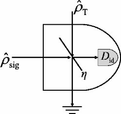
Figure 2: A model for an imperfect detector with efficiency $\eta$ and dark counts generated by a fictitious thermal background source. The signal mode and the thermal mode represented by the quantum states $\hat{\rho}_{\mbox{\tiny sig}}$ and $\hat{\rho}_{\mbox{\tiny T}}$, respectively, meet at a beamsplitter with transmittance $\eta$. One of its exits is directed to a perfect (ideal) detector ($D_{\mbox{\scriptsize id}}$), the photons of the second exit port are discarded. The perfect detector is assumed to be a unit-efficiency photon detector with no dark counts. We will make a distinction of two cases. In the first instance we will assume the perfect detector to be photon-number discriminating. Later we consider the case where the perfect detector is a unit-efficiency threshold detector.

The physical motivation behind this model is the association that the origin of dark counts stems from stray photons incident onto the detector from the environment. Furthermore, since the imperfect detector to be modeled has a non-unit efficiency, not all of the photons of the signal mode nor all photons from the thermal radiation cause a click in the detector, but just a fraction of them. This is effectively modeled by a beamsplitter whose transmittance $\eta$ is intended to represent the non-unit efficiency, followed by a subsequent perfect detector with unit-efficiency and no dark counts. Let us stress, however, that the thermal radiation intended to be responsible for dark counts is entirely fictitious and does not have to correspond to a real, actually existing photonic field. Any source of noise causing dark counts of the detector, e.g. electrical noise inside the detector, etc., can be effectively simulated by an imaginary thermal photonic field coupling into the detector from the environment via a beam splitter. This has been proven for homodyne detection by Appel et al. in Appel2007 .

As will be shown in the appendix A, the probability for a dark count in a non-ideal threshold detector amounts to

$$\wp_{\mbox{\tiny{dc}}}=\frac{(1-\eta)\tanh^{2}r}{1-\eta\tanh^{2}r}=\frac{(1-\eta)\exp[-\frac{\hbar\omega}{kT}]}{1-\eta\exp[-\frac{\hbar\omega}{kT}]}\;.$$ (23)

For any $0\leq\eta\leq 1$, we can always find a pseudo-temperature $T=T(r)$ to model any arbitrary value of $\wp_{\mbox{\tiny{dc}}}$. The case $\eta=1$ seems to exclude a non-vanishing $\wp_{\mbox{\tiny{dc}}}\not=0$. However, we may take the simultaneous limit $\eta\rightarrow 1$ and $T\rightarrow\infty$ in such a way that any dark count probability is kept fixed.

Using this detector model, we can calculate the conditional probability to detect $q\in{\mathbb{N}}_{0}$ photons with a photon-number discriminating detector possessing arbitrary efficiency $\eta$ and any dark count probability $\wp_{\mbox{\tiny{dc}}}$, given an input quantum state $\hat{\rho}_{\mbox{\tiny sig}}$ of the signal mode, according to:

$$p_{\eta,\wp_{\mbox{\tiny{dc}}}}(q|\hat{\rho}_{\mbox{\tiny sig}})=\mbox{Tr}_{\mbox{\tiny trans}}\left[\hat{\Pi}_{q}\mbox{Tr}_{\mbox{\tiny refl}}\left[\hat{U}_{\mbox{\tiny BS}}(\eta)\left(\hat{\rho}_{\mbox{\tiny sig}}\otimes\hat{\rho}_{\mbox{\tiny\em T}}\right)\hat{U}^{\dagger}_{\mbox{\tiny BS}}(\eta)\right]\hat{\Pi}_{q}\right]\;.$$ (24)

Again, we use the convention that “reflection” and “transmission” refer to the signal mode. Furthermore, throughout the article, the subscripts $\eta$ and $\wp_{\mbox{\tiny{dc}}}$ are used to express dependence on detector efficiency and dark count probability. For the purpose of this paper, it is sufficient to know the conditional probabilities for the particular input quantum states $\hat{\rho}_{\mbox{\tiny sig}}=|i\rangle\langle i|$, i.e. Fock states. We are therefore interested in $p_{\eta,\wp_{\mbox{\tiny{dc}}}}(q|i)$, with $i,q\in{\mathbb{N}}_{0}$, which is the conditional probability to detect $q$ photons given that $i$ photons are incident upon a photon-number discriminating detector with efficiency $\eta$ and dark count probability $\wp_{\mbox{\tiny{dc}}}$. Please note that now, due to dark counts, $q$ may be greater than $i$. A derivation of these probabilities constitutes a significant technical part of the present work and can be found in the appendix B. The result reads:

$$p_{\eta,\wp_{\mbox{\tiny{dc}}}}(q|i)=\left\{\begin{array}[]{ll}\frac{(1-\eta)(1-\wp_{\mbox{\tiny{dc}}})}{1-\eta(1-\wp_{\mbox{\tiny{dc}}})}\left(\frac{\eta}{1-\eta}\right)^{q}\left(1-\eta\right)^{i}G\left(i,q;\eta,\wp_{\mbox{\tiny{dc}}}\right)&\mbox{if $i\geq q$}\\ \frac{(1-\eta)(1-\wp_{\mbox{\tiny{dc}}})}{1-\eta(1-\wp_{\mbox{\tiny{dc}}})}\left[\frac{1-\eta}{\eta}b(\eta,\wp_{\mbox{\tiny{dc}}})\right]^{q-i}\eta^{i}G(q,i;\eta,\wp_{\mbox{\tiny{dc}}})&\mbox{if $q\geq i$}\\ \end{array}\right.\;\;,$$ (25)

where

$$b(\eta,\wp_{\mbox{\tiny{dc}}}):=\eta\tanh^{2}r\equiv\left[1+\frac{1-\eta}{\eta\wp_{\mbox{\tiny{dc}}}}\right]^{-1}\;,$$ (26)

and the function $G(\cdot,\cdot;\eta,\wp_{\mbox{\tiny{dc}}}):\mathbb{N}_{0}^{2}\rightarrow\mathbb{R}$ is given as follows. For $\kappa,\lambda\in{\mathbb{N}}_{0}$, $\kappa\geq\lambda$, we define:

$$G(\kappa,\lambda;\eta,\wp_{\mbox{\tiny{dc}}}):=\sum_{n=0}^{\infty}{\kappa\choose\lambda}{\kappa-\lambda+n\choose\kappa-\lambda}\left[b(\eta,\wp_{\mbox{\tiny{dc}}})\right]^{n}\left[\,{}_{2}F_{1}\left(-n,-\lambda\,;\kappa-\lambda+1\,;\frac{\eta-1}{\eta}\right)\right]^{2}\;,$$ (27)

and $G(\kappa,\lambda;\eta,\wp_{\mbox{\tiny{dc}}}):=0$ in the case $\kappa<\lambda$. Here and in what follows, ${}_{2}F_{1}(\cdot,\cdot,;\cdot\,;\cdot)$ denotes the Hypergeometric function which is defined as

$${}_{2}F_{1}(\alpha,\beta;\gamma;z) := 1+\sum_{n=1}^{\infty}\frac{(\alpha)_{n}(\beta)_{n}}{(\gamma)_{n}}\frac{z^{n}}{n!}\;\>,$$ (28)

where $(a)_{n}:=\Gamma(a+n)/\Gamma(a)$ is the Pochhammer symbol, and $\Gamma(\cdot)$ is the Gamma function. Please note that for $q=i$ the two results in Eq. (25) coincide.

II.3.4 Inefficient threshold detectors with dark counts

If we go a step further and acquiesce to the fact that photon-number discriminating detectors are a technological challenge and their realization is still in its infancy (however, see Rosenberg2005A ; Rosenberg2005B ), then, to provide a description of entanglement swapping of the most practical relevance, we have to consider threshold detectors BarlettSanders2002 . Ideally, such detectors effectively measure whether there are no photons or at least one photon in a mode. Following BarlettSanders2002 , we refer to a unit-efficiency threshold detector with no dark counts as an ideal threshold detector (ITD). Thus, an ITD is mathematically described by the PVM

$$\left\{\hat{\Pi}_{0}=|0\rangle\langle 0|\;,\;\hat{\Pi}_{>0}=\openone-\hat{\Pi}_{0}\right\}\;.$$ (29)

Inefficient threshold detectors with dark counts are contrived using the same detector model as above, but now with $D_{\mbox{\scriptsize id}}$ in Fig. 2 being an ITD instead of an ideal photon-counting detector. The relevant conditional probabilities are obtained in the same manner as above, using Eq. (24), but now with $q$ being either the event “no click” or the complementary event “click”, corresponding to the PVM elements $\hat{\Pi}_{0}$ or $\hat{\Pi}_{>0}$, respectively. Again, for the purpose of entanglement swapping, we would like to know these conditional probabilities particularly for the signal input quantum states $\hat{\rho}_{\mbox{\tiny sig}}=|i\rangle\langle i|$. The conditional probability of recording “no click” by a threshold detector with efficiency $\eta$ and dark count probability $\wp_{\mbox{\tiny{dc}}}$ given that $i$ photons are incident upon it, can be directly obtained from the result (25) by setting $q=0$. And the probability for the complementary event “click” is just one minus the latter probability:

$$p_{\eta,\wp_{\mbox{\tiny{dc}}}}(\mbox{``no click"}|i) = p_{\eta,\wp_{\mbox{\tiny{dc}}}}(q=0|i)$$ (30)

$$= (1-\wp_{\mbox{\tiny{dc}}})\big{[}1-\eta(1-\wp_{\mbox{\tiny{dc}}})\big{]}^{i}$$

$$p_{\eta,\wp_{\mbox{\tiny{dc}}}}(\mbox{``click"}|i) = 1-p_{\eta,\wp_{\mbox{\tiny{dc}}}}(\mbox{``no click"}|i)$$ (31)

$$= 1-(1-\wp_{\mbox{\tiny{dc}}})\big{[}1-\eta(1-\wp_{\mbox{\tiny{dc}}})\big{]}^{i}$$

II.3.5 Bayesian updating based on evidence obtained by imperfect detectors

In order to provide the resultant mixed quantum state of the remaining modes $a$ and $d$ depending on the result $(qrst)$ of a Bell-state measurement on the $c$ and $b$ modes with imperfect detectors including the presence of dark counts, we proceed in the fashion of Bayesian inference and reasoning. We first assume the notional ideal situation that the detectors used for the Bell-state measurement are unit-efficiency photon-number discriminating detectors with no dark counts. In this hypothetical case we know how to calculate the probability for a certain measurement readout $(ijkl)$ of the perfectly accurate Bell-state measurement as well as the corresponding resultant pure quantum state, denoted by $|\Phi_{ijkl}\rangle$, of the remaining modes $a$ and $d$ after the measurement, using von Neumann’s projection postulate vonNeumann1932 . We use this information as our hypothesis prior to observing evidence in the real experiment. The probability $p(ijkl)$ is our prior probability of the hypothesis that the resultant quantum state of the remaining modes $a$ and $d$ after the Bell measurement is given by $|\Phi_{ijkl}\rangle$.

Before we proceed, we would like to make the following agreement. Throughout the paper we agree upon using the letters $q,r,s,t$ to denote the readouts of measurements using imperfect detectors, and the letters $i,j,k,l$ to label results of hypothetical measurements employing perfect photon-number discriminating detectors. As for imperfect detectors, we differentiate between photon-number discriminating detectors and threshold detectors. In the first case $q,r,s,t\in{\mathbb{N}}_{0}$, in the latter case $q,r,s,t\in\{\mbox{\em``no click''},\mbox{\em``click''}\}$.

Given an actual detector readout $(qrst)$ of an imperfect Bell measurement with inaccurate detectors including the presence of dark counts, we infer what an ideal four-tuple of detectors would have yielded, i.e., readout $(ijkl)$, with probability $P^{qrst}_{ijkl}:=p(ijkl|qrst)$. In the language of Bayesianism, after the evidence $(qrst)$ has been observed by an imperfect Bell measurement, we update our knowledge with regard to the hypothesis according to Bayes’ theorem, by means of which we can calculate the posterior probability of the hypothesis $(ijkl)$ given the obtained evidence $(qrst)$:

$$P^{qrst}_{ijkl} \equiv p(ijkl|qrst)=\frac{p(qrst|ijkl)p(ijkl)}{p(qrst)}$$ (32)

$$= \frac{p(qrst|ijkl)p(ijkl)}{\sum_{i^{\prime},j^{\prime},k^{\prime},l^{\prime}=0}^{\infty}p(qrst|i^{\prime}j^{\prime}k^{\prime}l^{\prime})p(i^{\prime}j^{\prime}k^{\prime}l^{\prime})}\;.$$

Here, $p(qrst|ijkl)$ indicates the conditional probability for obtaining the evidence $(qrst)$ given that the hypothesis $(ijkl)$ would have happened to be true, if the detectors of our Bell-state measurement had been ideal. It is important to realize that $p(qrst|ijkl)$ is equivalent to the conditional probability of recording the readout $(qrst)$ given that exactly $i$, $j$, $k$ and $l$ photons are incident onto the four non-ideal detectors of the Bell-state measurement. Hence, the resultant quantum state of the remaining modes $a$ and $d$ after recording the actual readout $(qrst)$ at the inefficient detectors, is a mixed state of the form

$$\hat{\rho}^{qrst}=\sum_{ijkl}P^{qrst}_{ijkl}|\Phi_{ijkl}\rangle\langle\Phi_{ijkl}|\;.$$ (33)

In the next section we provide closed-form expressions for the conditional probabilities $P^{qrst}_{ijkl}$ depending on the experimental parameters $\chi$, $\eta$ and $\wp_{\mbox{\tiny{dc}}}$. In the first instance we assume imperfect photon-number discriminating detectors, i.e. detectors that realize a photon-counting PVM but are in general inefficient ($\eta\leq 1$), and have a non-zero dark-count probability $\wp_{\mbox{\tiny{dc}}}\not=0$. As our next step we consider imperfect threshold detectors. Again, in the style of Bayesian reasoning we upgrade our probabilities of the density operator (33) using the evidence that the measurement outcomes $q,r,s,t$ of a Bell-state measurement with threshold detectors can be either “no click” or “click”. The resultant quantum state obtained in this way is the most relevant result, as it refers to the most common practical situation, namely entanglement swapping using ordinary inaccurate threshold detectors.

II.4 Quantum state after entanglement swapping

Using the tools presented in the previous sections we are now in a position to derive the resultant quantum state (33) after a realistic entanglement swapping with imperfect sources and imperfect detectors.

We start with the quantum state provided by the two PDC sources, Eq. (16). Suppose our four detectors of the Bell measurement on the modes $b$ and $c$ were perfect, i.e., had a unit-efficiency $\eta=1$ and no detector dark counts. Then, to give the ideal readout $(ijkl)$, after applying the balanced beamsplitter transformation $B=\frac{1}{\sqrt{2}}\left({\;\,1\atop-1}{1\atop 1}\right)$ to modes $b$ and $c$ using the rule VogelWelsch2006

$${\hat{b}_{\mbox{\tiny{H}}}\choose\hat{c}_{\mbox{\tiny{H}}}}\rightarrow B^{\dagger}{\hat{b^{\prime}}_{\mbox{\tiny{H}}}\choose\hat{c^{\prime}}_{\mbox{\tiny{H}}}}\quad,\quad{\hat{b}^{\dagger}_{\mbox{\tiny{H}}}\choose\hat{c}^{\dagger}_{\mbox{\tiny{H}}}}\rightarrow B^{T}{\hat{b^{\prime}}^{\dagger}_{\mbox{\tiny{H}}}\choose\hat{c^{\prime}}^{\dagger}_{\mbox{\tiny{H}}}}\;,$$ (34)

and similarly for the vertical polarization, the resulting four-mode quantum state $\hat{U}_{B}|\chi\rangle$ is to be projected onto the subspace corresponding to the projector

$$\hat{\Pi}^{(ijkl)}_{c^{\prime}_{H},c^{\prime}_{V},b^{\prime}_{V},b^{\prime}_{H}}:=\left(|i\rangle\langle i|\right)_{c^{\prime}_{H}}\otimes(|j\rangle\langle j|)_{c^{\prime}_{V}}\otimes(|k\rangle\langle k|)_{b^{\prime}_{V}}\otimes(|l\rangle\langle l|)_{b^{\prime}_{H}}\otimes\openone_{a_{H}}\otimes\openone_{a_{V}}\otimes\openone_{d_{V}}\otimes\openone_{d_{H}}\;.$$ (35)

The modes $c^{\prime}_{H},c^{\prime}_{V},b^{\prime}_{V}$ and $b^{\prime}_{H}$ are the output modes of the balanced beamsplitter, cf. Fig. 1. The operator $\hat{U}_{B}$ represents the unitary evolution corresponding to the beamsplitter transformation in the Schrödinger picture, which we use. Here and in what follows, $|n\rangle$ denotes an $n$-photon Fock state. It should be clear from the context to which mode it refers. Accordingly, $(|i\rangle\langle i|)_{c^{\prime}_{H}}$ represents a projection operator corresponding to the Fock state $|i\rangle$ of mode $c^{\prime}_{H}$, etc.. The projection (35) followed by state normalization yields the following post-measurement quantum state :

$$\frac{\hat{\Pi}^{(ijkl)}_{c^{\prime}_{H},c^{\prime}_{V},b^{\prime}_{V},b^{\prime}_{H}}\hat{U}_{B}|\chi\rangle}{\left\|\hat{\Pi}^{(ijkl)}_{c^{\prime}_{H},c^{\prime}_{V},b^{\prime}_{V},b^{\prime}_{H}}\hat{U}_{B}|\chi\rangle\right\|}=|i^{c^{\prime}_{H}}\,j^{c^{\prime}_{V}}\,k^{b^{\prime}_{V}}\,l^{b^{\prime}_{H}}\rangle\otimes|\Phi_{ijkl}\rangle\;,$$ (36)

with the first factor being the Fock state with $i,j,k,l$ photons in the modes $c^{\prime}_{H}$, $c^{\prime}_{V}$, $b^{\prime}_{V}$, and $b^{\prime}_{H}$, respectively, and

$$|\Phi_{ijkl}\rangle \equiv \frac{1}{\sqrt{i!j!k!l!}}\left(\frac{\hat{d}_{\mbox{\tiny{H}}}^{\dagger}-\hat{a}_{\mbox{\tiny{H}}}^{\dagger}}{\sqrt{2}}\right)^{i}\left(\frac{\hat{d}_{\mbox{\tiny{V}}}^{\dagger}-\hat{a}_{\mbox{\tiny{V}}}^{\dagger}}{\sqrt{2}}\right)^{j}\left(\frac{\hat{a}_{\mbox{\tiny{V}}}^{\dagger}+\hat{d}_{\mbox{\tiny{V}}}^{\dagger}}{\sqrt{2}}\right)^{k}\left(\frac{\hat{a}_{\mbox{\tiny{H}}}^{\dagger}+\hat{d}_{\mbox{\tiny{H}}}^{\dagger}}{\sqrt{2}}\right)^{l}|\mbox{vac}\rangle$$

$$= \frac{1}{(\sqrt{2})^{i+j+k+l}\sqrt{i!j!k!l!}}\sum_{\mu=0}^{i}\sum_{\nu=0}^{j}\sum_{\kappa=0}^{k}\sum_{\lambda=0}^{l}(-1)^{\mu+\nu}{i\choose\mu}{j\choose\nu}{k\choose\kappa}{l\choose\lambda}$$

$$\times\left(\hat{a}_{\mbox{\tiny{H}}}^{\dagger}\right)^{\mu+\lambda}\left(\hat{a}_{\mbox{\tiny{V}}}^{\dagger}\right)^{\nu+\kappa}\left(\hat{d}_{\mbox{\tiny{H}}}^{\dagger}\right)^{i+l-\mu-\lambda}\left(\hat{d}_{\mbox{\tiny{V}}}^{\dagger}\right)^{j+k-\nu-\kappa}|\mbox{vac}\rangle\;.$$

Since the photons of the $c$ and $b$ modes are destroyed in the measurement process, we discard the first factor of Eq. (36). The second factor, $|\Phi_{ijkl}\rangle$, is the resultant pure state of the remaining $a$ and $d$ modes: The corresponding probability of the hypothetical ideal measurement readout $(ijkl)$ is given by:

$$p(ijkl)=\,\left\|\hat{\Pi}^{(ijkl)}_{c^{\prime}_{H},c^{\prime}_{V},b^{\prime}_{V},b^{\prime}_{H}}\hat{U}_{B}|\chi\rangle\right\|^{2}=\frac{\big{[}\tanh\chi\big{]}^{2(i+j+k+l)}}{\cosh^{8}\chi}\;.$$ (38)

In an actual experiment, however, detectors have an efficiency which is appreciably less than 100% and in addition exhibit dark counts. Given an actual detector readout $(qrst)$ of an imperfect Bell measurement with faulty photon-number discriminating detectors characterized by efficiency $\eta<1$ and dark count probability $\wp_{\mbox{\tiny{dc}}}$, we do not know the corresponding resultant post-measurement pure quantum state for the remaining $a$ and $d$ modes nor the probability of its occurrence. We can, however, calculate the posterior conditional probability for any readout $(ijkl)$ an ideal four-tuple of detectors would have yielded, i.e., the probability $P^{qrst}_{ijkl}(\eta,\wp_{\mbox{\tiny{dc}}})\equiv p_{\eta,\wp_{\mbox{\tiny{dc}}}}(ijkl|qrst)$. As explained in the previous section, this is done using Bayes’ theorem (32), according to which we achieve our goal if we know the conditional probabilities $p_{\eta,\wp_{\mbox{\tiny{dc}}}}(qrst|ijkl)$ for all possible events $(ijkl)\in{\mathbb{N}}_{0}^{4}$. Since the four detectors are statistically independent from one another, these probabilities factorize into four terms:

$$p_{\eta,\wp_{\mbox{\tiny{dc}}}}(qrst|ijkl)=p_{\eta,\wp_{\mbox{\tiny{dc}}}}(q|i)\,p_{\eta,\wp_{\mbox{\tiny{dc}}}}(r|j)\,p_{\eta,\wp_{\mbox{\tiny{dc}}}}(s|k)\,p_{\eta,\wp_{\mbox{\tiny{dc}}}}(t|l)\;,$$ (39)

where each of these factors is given by the expression (25). The factorization of the conditional probabilities together with result (38) imply a factorization of the posterior probabilities of Eq. (32):

$$P^{qrst}_{ijkl}(\chi,\eta,\wp_{\mbox{\tiny{dc}}})=f^{q}_{i}(\chi,\eta,\wp_{\mbox{\tiny{dc}}})f^{r}_{j}(\chi,\eta,\wp_{\mbox{\tiny{dc}}})f^{s}_{k}(\chi,\eta,\wp_{\mbox{\tiny{dc}}})f^{t}_{l}(\chi,\eta,\wp_{\mbox{\tiny{dc}}})\;,$$ (40)

where we now explicitely express their dependence on the experimental parameters $\chi,\eta$ and $\wp_{\mbox{\tiny{dc}}}$. By inserting result (38) and our physical assumption (39) into (32), we have:

$$f^{q}_{i}(\chi,\eta,\wp_{\mbox{\tiny{dc}}})\equiv\frac{p_{\eta,\wp_{\mbox{\tiny{dc}}}}(q|i)\tanh^{2i}\chi}{\sum_{i^{\prime}=0}^{\infty}p_{\eta,\wp_{\mbox{\tiny{dc}}}}(q|i^{\prime})\tanh^{2i^{\prime}}(\chi)}$$ (41)

and equivalent formulae for $f^{r}_{j}(\chi,\eta,\wp_{\mbox{\tiny{dc}}})$, $f^{s}_{k}(\chi,\eta,\wp_{\mbox{\tiny{dc}}})$ and $f^{t}_{l}(\chi,\eta,\wp_{\mbox{\tiny{dc}}})$. By inserting (25) into (41) we finally obtain the following exact closed-form solution:

$$f^{q}_{i}(\chi,\eta,\wp_{\mbox{\tiny{dc}}})=\left\{\begin{array}[]{ll}\frac{\tanh^{2i}(\chi)(1-\eta)^{i-q}G(i,q;\eta,\wp_{\mbox{\tiny{dc}}})}{g(q;\chi,\eta,\wp_{\mbox{\tiny{dc}}})}&\mbox{if $i\geq q$}\\ \frac{\tanh^{2i}(\chi)\eta^{2(i-q)}(1-\eta)^{q-i}b^{q-i}(\eta,\wp_{\mbox{\tiny{dc}}})G(q,i;\eta,\wp_{\mbox{\tiny{dc}}})}{g(q;\chi,\eta,\wp_{\mbox{\tiny{dc}}})}&\mbox{if $q\geq i$}\\ \end{array}\right.$$ (42)

with the common denominator

$$g(q;\chi,\eta,\wp_{\mbox{\tiny{dc}}}) := \sum_{i^{\prime}=0}^{q}\tanh^{2i^{\prime}}(\chi)\,\eta^{2(i^{\prime}-q)}(1-\eta)^{q-i^{\prime}}b^{q-i^{\prime}}(\eta,\wp_{\mbox{\tiny{dc}}})G(q,i^{\prime};\eta,\wp_{\mbox{\tiny{dc}}})$$ (43)

$$+\sum_{i^{\prime}=q+1}^{\infty}\tanh^{2i^{\prime}}(\chi)(1-\eta)^{i^{\prime}-q}G(i^{\prime},q;\eta,\wp_{\mbox{\tiny{dc}}})$$

and similar expressions for $f^{r}_{j}(\chi,\eta,\wp_{\mbox{\tiny{dc}}})$, $f^{s}_{k}(\chi,\eta,\wp_{\mbox{\tiny{dc}}})$ and $f^{t}_{l}(\chi,\eta,\wp_{\mbox{\tiny{dc}}})$. Eqs. (40),(42) and (43) form our result for photon-number discriminating detectors. Knowing the probabilities $P^{qrst}_{ijkl}(\chi,\eta,\wp_{\mbox{\tiny{dc}}})$ for all possible hypothetical readouts $(ijkl)$ with $i,j,k,l\in\mathbb{N}_{0}$ allows computation of the mixed quantum state (33) for the remaining $a$ and $d$ modes after an imperfect Bell measurement with measurement result $(qrst)$ using photon-number discriminating detectors with efficiency $\eta$ and dark count probability $\wp_{\mbox{\tiny{dc}}}$.

Let us consider the special case when dark counts are absent, i.e. $\wp_{\mbox{\tiny{dc}}}=0$. With Eq. (23) this leads to $(1-\eta)\tanh^{2}r=0$ and therefore $\tanh^{2}r=0$ as $\eta\not=1$ in general. This in turn implies $b(\eta,\wp_{\mbox{\tiny{dc}}}=0)=\eta\tanh^{2}r\equiv 0$ as $\eta\not=0$, and as a consequence also $G(\kappa,\lambda;\eta,\wp_{\mbox{\tiny{dc}}}=0)={\kappa\choose\lambda}$. According to our general result (42) the absence of dark counts, $\wp_{\mbox{\tiny{dc}}}=0$, implies $i\geq q$, again as $b(\eta,\wp_{\mbox{\tiny{dc}}}=0)$ must be zero, and we obtain:

$$f^{q}_{i}(\chi,\eta,\wp_{\mbox{\tiny{dc}}}=0) = \frac{{i\choose q}(1-\eta)^{i-q}\tanh^{2i}\chi}{\sum_{i^{\prime}=q}^{\infty}{i^{\prime}\choose q}(1-\eta)^{i^{\prime}-q}\tanh^{2i^{\prime}}\chi}$$ (44)

$$= \frac{{i\choose q}(1-\eta)^{i-q}\big{[}\tanh^{2}\chi\big{]}^{i-q}}{\sum_{i"=0}^{\infty}{q+i"\choose q}\big{[}(1-\eta)\tanh^{2}\chi\big{]}^{i"}}$$

$$= \frac{{i\choose q}\big{[}\tanh^{2}\chi\big{]}^{i-q}(1-\eta)^{i-q}}{\frac{1}{\Big{(}1-\big{[}(1-\eta)\tanh^{2}\chi\big{]}\Big{)}^{q+1}}}\;,$$

i.e., we get the result:

$$f^{q}_{i}(\chi,\eta,\wp_{\mbox{\tiny{dc}}}=0)={i\choose q}\big{[}(1-\eta)\tanh^{2}\chi\big{]}^{i-q}\Big{(}1-\big{[}(1-\eta)\tanh^{2}\chi\big{]}\Big{)}^{q+1}\;.$$ (45)

If we also let the efficiency $\eta$ go to unity, $\eta\rightarrow 1$, we arrive at:

$$\lim_{\eta\rightarrow 1}f^{q}_{i}(\chi,\eta,\wp_{\mbox{\tiny{dc}}}=0)=\delta_{qi}\;,$$ (46)

where $\delta_{qi}$ is the Kronecker delta symbol. This is also what one should expect in the ideal case of perfect detectors with no dark counts. Please note, that with $\eta\rightarrow 1$ we have also implicitly assumed that there are no transmission losses between the sources and detectors.

Acquiescing to the fact that photon-number discriminating detectors are still a technological challenge, we now consider the more practical situation of threshold detectors, in which case the events $(qrst)$ of the Bell measurement consist of readouts $q,r,s,t\in\{\mbox{\em``no click''},\mbox{\em``click''}\}$. The conditional probabilities are given by (30) and (31). Calculation of the functions $f^{q}_{i}(\chi,\eta,\wp_{\mbox{\tiny{dc}}})$ in Eq. (41) yields the following result:

$$f^{\mbox{\tiny``no click"}}_{i}(\chi,\eta,\wp_{\mbox{\tiny{dc}}}) = \big{[}h(\chi,\eta,\wp_{\mbox{\tiny{dc}}})\big{]}^{i}\big{(}1-h(\chi,\eta,\wp_{\mbox{\tiny{dc}}})\big{)}\;,$$ (47)

$$f^{\mbox{\tiny``click"}}_{i}(\chi,\eta,\wp_{\mbox{\tiny{dc}}}) = \frac{\Big{\{}\tanh^{2i}\chi-(1-\wp_{\mbox{\tiny{dc}}})\left[h(\chi,\eta,\wp_{\mbox{\tiny{dc}}})\right]^{i}\Big{\}}}{\cosh^{2}\chi-\frac{1-\wp_{\mbox{\tiny{dc}}}}{1-h(\chi,\eta,\wp_{\mbox{\tiny{dc}}})}}\;,$$ (48)

where we have introduced the definition:

$$h(\chi,\eta,\wp_{\mbox{\tiny{dc}}}):=\left[1-\eta(1-\wp_{\mbox{\tiny{dc}}})\right]\tanh^{2}\chi\;.$$ (49)

Eq. (40) together with (47 -49) form our result for threshold detectors. Please note, that in the ideal case, $\eta=1$ and $\wp_{\mbox{\tiny{dc}}}=0$, our result reduces to what we should expect:

$$f^{\mbox{\tiny``no click"}}_{i}(\chi,\eta=1,\wp_{\mbox{\tiny{dc}}}=0)=\delta_{i,0}$$ (50)

and

$$f^{\mbox{\tiny``click"}}_{i}(\chi,\eta=1,\wp_{\mbox{\tiny{dc}}}=0) = \left\{\begin{array}[]{ll}0&\quad\mbox{if $i=0$}\\ \frac{\tanh^{2i}\chi}{\sinh^{2}\chi}&\quad\mbox{if $i\geq 1$}\\ \end{array}\right.$$ (53)

$$\sum_{i=1}^{\infty}f^{\mbox{\tiny``click"}}_{i}(\chi,\eta=1,\wp_{\mbox{\tiny{dc}}}=0) = \frac{\tanh^{2}\chi}{\sinh^{2}\chi}\sum_{i^{\prime}=0}^{\infty}\tanh^{2i^{\prime}}\chi=1\;.$$ (54)

As for the peculiar non-relevant marginal situation $\eta=0$ and $\wp_{\mbox{\tiny{dc}}}=0$, we note that in this case there can be no click events, so that $f^{\mbox{\tiny``click"}}_{i}(\chi,\eta=0,\wp_{\mbox{\tiny{dc}}}=0)$ becomes a meaningless conditional probability. So it is not a flaw that the latter is not defined in this marginal situation. On the other hand, we get $f^{\mbox{\tiny``no click"}}_{i}(\chi,\eta=0,\wp_{\mbox{\tiny{dc}}}=0)=\tanh^{2i}\chi/\cosh^{2}\chi$ and $\sum_{i=0}^{\infty}f^{\mbox{\tiny``no click"}}_{i}(\chi,\eta=0,\wp_{\mbox{\tiny{dc}}}=0)=1$.

Our derivation of the resultant quantum state (33) after an imperfect entanglement swapping is based on Bayesian reasoning and the physical assumption that the four detectors of the Bell-state measurement are statistically independent from one another implying the property of Eq. (39). The latter property involves a factorization of the probabilities $P^{qrst}_{ijkl}$ into four terms corresponding to the four independent detectors, cf. Eq. (40). An obvious generalization of our results is to allow different efficiencies as well as different dark count probabilities for the four detectors. The derivation is very similar and the result reads:

$$P^{qrst}_{ijkl}(\,\chi,\{\eta_{\nu}\},\{{\wp_{\mbox{\tiny{dc}}}}_{\nu}\})=f^{q}_{i}(\chi,\eta_{1},{\wp_{\mbox{\tiny{dc}}}}_{1})f^{r}_{j}(\chi,\eta_{2},{\wp_{\mbox{\tiny{dc}}}}_{2})f^{s}_{k}(\chi,\eta_{3},{\wp_{\mbox{\tiny{dc}}}}_{3})f^{t}_{l}(\chi,\eta_{4},{\wp_{\mbox{\tiny{dc}}}}_{4})\;,$$ (55)

where $\eta_{\nu}$ and ${\wp_{\mbox{\tiny{dc}}}}_{\nu}$, $\nu=1,2,3,4$, denote the arbitrary and in general different efficiencies and dark count probabilities of the four detectors. The functions $f^{m}_{n}(\chi,\eta_{\nu},{\wp_{\mbox{\tiny{dc}}}}_{\nu})$ are given either by the result (42) in the case of photon-number discriminating detectors or by (47,48) in the case of threshold detectors.

III Comparison with experimental entanglement swapping

To evaluate the value of our model we test it against results of real entanglement swapping experiments PanBouwmeesterWeinfurterZeilinger1998 ; JenneweinWeihsPanZeilinger2002 ; RiedmattenMarcikicHouwelingenTittelZbindenGisin2005 . In these experiments entanglement verification is accomplished either by observing the visibility of four-fold coincidences of four threshold detectors (two for the Bell-state measurement and two for monitoring the modes $a$ and $d$, one on each side), obtained via variable polarization directions of analyzers, or by measuring certain correlation coefficients for polarization related to tests of the CHSH Bell inequality Clauser1969 . Assuming the resultant quantum state of the photons of the remaining modes $a$ and $d$ to be given by a Werner state, cf. Tittel2003 ,

$$\hat{\rho}^{qrst}=F|\psi^{T}\rangle\langle\psi^{T}|+\frac{1-F}{3}\left(\openone-|\psi^{T}\rangle\langle\psi^{T}|\right)\;,$$ (56)

where $|\psi^{T}\rangle$ is some target Bell state, the visibility is directly connected to the fidelity $F=\langle\psi^{T}|\hat{\rho}^{qrst}|\psi^{T}\rangle$ via the relation (cf. RiedmattenMarcikicHouwelingenTittelZbindenGisin2005 ):

$$V=(4F-1)/3\;.$$ (57)

Let us emphasize, however, that the assumption (56) is justified only for the post-selected quantum state $\hat{\rho}^{qrst}_{\mbox{\tiny postsel}}$, i.e, provided that click events are observed in both the $a$ and $d$ modes. This issue will be clarified below. The visibility is obtained according to $V=\left(\mbox{Max}-\mbox{Min}\right)/\left(\mbox{Max}+\mbox{Min}\right)$, where “Max” and “Min” denote the maximal and minimal values of the four-fold coincidence rate as a function of some polarization angle, respectively. The relation between visibility and the correlation coefficient $S$ of the CHSH Bell inequality is $S=2\sqrt{2}\,V$, cf. Rarity1990 .

To simulate a four-fold coincidence experiment and provide predictions for the visibility we proceed as follows. In accordance with the experimental situation of references PanBouwmeesterWeinfurterZeilinger1998 ; RiedmattenMarcikicHouwelingenTittelZbindenGisin2005 we choose to consider four-fold coincidence events in which the result of the Bell measurement on the $b$ and $c$ modes corresponds — in the ideal case scenario — to a projection onto the Bell state

$$|\Psi^{-}\rangle_{cb}=\frac{1}{\sqrt{2}}\left(\hat{c}_{\mbox{\tiny{H}}}^{\dagger}\hat{b}_{\mbox{\tiny{V}}}^{\dagger}-\hat{c}_{\mbox{\tiny{V}}}^{\dagger}\hat{b}_{\mbox{\tiny{H}}}^{\dagger}\right)|\mbox{vac}\rangle\;.$$ (58)

According to the common argument on entanglement swapping, this would mean that the remaining modes $a$ and $d$ are left in the same Bell state, i.e.  $|\Psi^{-}\rangle_{ad}$. To verify this entangled state by measurements on the $a$ and $d$ modes is the objective of the experiment of PanBouwmeesterWeinfurterZeilinger1998 . The experimental situations in references JenneweinWeihsPanZeilinger2002 ; RiedmattenMarcikicHouwelingenTittelZbindenGisin2005 are very similar.

Let us for a moment assume that our detectors and sources are ideal. Then, a projection onto the Bell state $|\Psi^{-}\rangle_{cb}$ is achieved whenever there are coincidence clicks of the two detectors for the $c^{\prime}_{H}$ and the $b^{\prime}_{V}$ mode or, vice versa, of the two detectors for the $c^{\prime}_{V}$ and $b^{\prime}_{H}$ modes. To understand this issue, we can exploit the fact that the Bell state $|\Psi^{-}\rangle_{cb}$ is antisymmetric under exchange of labels $c$ and $b$ implying fermionic statistics in the spatial behavior of the two photons, which means that they have to emerge from different ports of the balanced beam-splitter (cf. Fig. 1). The other three Bell states are symmetric with respect to exchange of labels $c$ and $b$ involving bosonic statistics in the spatial behavior, meaning that the photons will emerge at the same output port of the beamsplitter. Hence, in the ideal case of perfect sources and detectors, observing coincidences between two detectors on both sides of the beamsplitter is an experimental evidence for a projection onto the state $|\Psi^{-}\rangle_{cb}$ and thus also a preparation of the state $|\Psi^{-}\rangle_{ad}$ for the $a$ and $d$ modes. Only the coincidences of “$c^{\prime}_{H}$ and $b^{\prime}_{V}$” or “$c^{\prime}_{V}$ and $b^{\prime}_{H}$” clicks are possible, but not of two clicks corresponding to the same polarization, i.e., “$c^{\prime}_{H}$ and $b^{\prime}_{H}$” or “$c^{\prime}_{V}$ and $b^{\prime}_{V}$”, since the polarizations in the Bell state $|\Psi^{-}\rangle_{cb}$ are anti-correlated.

Yet, in a real experiment scenario the PDC sources and detectors are not ideal. In particular, we have to allow for the rare but non-negligible faulty events due to emission of multi-photon pairs as well as dark counts, and also take into account transmission losses and detector inefficiencies, so that the actual quantum state of the remaining $a$ and $d$ modes after the suggested Bell measurement will deviate from $|\Psi^{-}\rangle_{ad}$. Within the setting of our model with imperfect threshold detectors, a non-ideal projection onto the Bell state $|\Psi^{-}\rangle_{cb}$ is achieved whenever one of the following Bell measurement events $(q,r,s,t)$ is obtained: $(1,0,1,0)$ or $(0,1,0,1)$. Here and in what follows, $q=1$ means a click and $q=0$ that the detector does not click.

Before we proceed we would like to comment on the following interesting observation. Even if the detectors of the Bell-state measurement were ideal ($\eta=1,\wp_{\mbox{\tiny{dc}}}=0$), they would never indicate a projection onto $|\Psi^{-}\rangle_{cb}$ and as a consequence prepare the Bell state $|\Psi^{-}\rangle_{ad}$ unless also the photon-pair sources were ideal. The multi-pair nature of the PDC sources precludes a projection onto the Bell state $|\Psi^{-}\rangle_{cb}$ regardless of the quality of the detectors used for the Bell-state measurement. To understand this feature, let us consider the outcome $(1010)$ of the Bell-state measurement on the $b$ and $c$ modes and assume ideal photon-number discriminating detectors. In this situation, according to Eq. (46), we have $P^{qrst}_{ijkl}=\delta_{qi}\delta_{rj}\delta_{sk}\delta_{tl}$ and the quantum state (33) reduces to a single component, namely the pure state $|\Phi_{1010}\rangle$. According to (II.4) we obtain

$$|\Phi_{1010}\rangle=\frac{1}{\sqrt{2}}\left(\frac{|1010\rangle-|0101\rangle}{\sqrt{2}}+\frac{|0011\rangle-|1100\rangle}{\sqrt{2}}\right)\;.$$ (59)

Thus, apart from the expected Bell state $|\psi^{-}\rangle_{ad}\,$, we get another term superposed to it, namely a superposition of two photons being in the $a$ mode (in different polarizations of the latter) and no photons in the $d$ mode and vice versa. This is also understandable intuitively. There are three quantum alternatives contributing to the event $(qrst)=(1010)$ of the Bell measurement: (i) each PDC source emits exactly one photon-pair; ($ii$) the “first” PDC source produces vacuum and the “second” source two (independent) photon pairs; ($iii$) the “first” PDC source produces two photon pairs and the “second” source vacuum. The probability of each of these three alternatives is proportional to $\chi^{4}$, which also explains why the resultant normalized quantum state (59) of the remaining modes $a$ and $d$ does not depend on $\chi$. Only the alternative ($i$) leads to the desired Bell state $|\psi^{-}\rangle_{ad}$, whereas the other two alternatives ($ii$) and ($iii$) entail the second term in (59). For this feature see also Riedmatten2003Phys.Rev.A67 .

Hence, entanglement swapping performed with PDC sources cannot herald Bell states in the outgoing modes with a 100% probability, even if the detectors used for the Bell measurement are perfectly ideal. If, however, we are interested in post-selected correlations of detection events of the $a$ and $d$ modes, only the Bell state $|\psi^{-}\rangle_{ad}$ contributes to them. And as expected, the detection events will be perfectly anti-correlated. The second term in Eq. (59) does not contribute to four-fold coincidences and thus can be ignored in terms of post-selection. Furthermore, to fulfill the commonly used relation (57) between the fidelity and the experimentally observed visibility of four-fold coincidences, the former has to be calculated with the post-selected state. This means we have to project the quantum state $\hat{\rho}^{qrst}$ onto the subspace which corresponds to click events in both the $a$ and $d$ modes. Each of the outgoing modes has to have at least one photon. Introducing the projection operator

$$\hat{\Pi}_{\mbox{\tiny postsel}}:=\left(\openone_{a_{H},a_{V}}-\left(|00\rangle\langle 00|\right)_{a_{H},a_{V}}\right)\otimes\left(\openone_{d_{V},d_{H}}-\left(|00\rangle\langle 00|\right)_{d_{V},d_{H}}\right)\;,$$ (60)

the post-selected quantum state is defined as:

$$\hat{\rho}^{qrst}_{\mbox{\tiny postsel}}:=\frac{\hat{\Pi}_{\mbox{\tiny postsel}}\hat{\rho}^{qrst}\hat{\Pi}_{\mbox{\tiny postsel}}}{\mbox{Tr}[\hat{\Pi}_{\mbox{\tiny postsel}}\hat{\rho}^{qrst}\hat{\Pi}_{\mbox{\tiny postsel}}]}\;.$$ (61)

The fidelity

$$F_{\mbox{\tiny postsel}}:=\langle\psi^{-}|\hat{\rho}^{qrst}_{\mbox{\tiny postsel}}|\psi^{-}\rangle\;.$$ (62)

fulfills the relation (57), (see RiedmattenMarcikicHouwelingenTittelZbindenGisin2005 ).

Our scheme for entanglement verification via four-fold coincidence measurements is very similar to the experimental setup in PanBouwmeesterWeinfurterZeilinger1998 . It is illustrated in Fig. 3. We implement variable polarization measurements on both modes $a$ and $d$ by introducing polarization rotators (PR) into their spatial paths prior to polarizing beam-splitters and threshold detectors. The polarizations of the $a$ and $d$ modes are rotated by independently variable angles $\alpha$ and $\delta$. To avoid any confusion, let us agree upon the following meaning of the latter. The angles $\alpha$ and $\delta$ stand for rotation angles of polarization vectors in the real space and not of Bloch vectors on the Bloch sphere. Neither do they mean rotation angles of the $\lambda/2$-plates, which are used in an actual experiment to cause polarization rotations. The relation between these three different meanings is as follows. A rotation by angle $\alpha$ of a polarization vector in real space corresponds to a rotation by angle $\tilde{\alpha}=2\alpha$ of the Bloch vector on the Bloch sphere and to a rotation by angle $\alpha_{\lambda/2}=\alpha/2$ of the $\lambda/2$-plate.

Polarization rotations prior to PBS separating horizontal and vertical polarizations, and photon-detections, are equivalent to polarization measurements in different bases in Hilbert space. The absolute angle of rotation in each of the modes determines the basis of the polarization measurement. The polarization correlations of the entangled state should, in the ideal-case scenario, depend only on the relative angle between the two polarization rotators. We choose to rotate the polarization of mode $a$ by a fixed angle $\alpha=\pi/4$ (i.e. $+45^{\circ}$) and numerically calculate the probabilities for coincidences of detector clicks for measurements on the $a$ and $d$ modes, for varying angles $\delta$ of polarization rotation of the $d$ mode, given that the Bell measurement has yielded the result $(1,0,1,0)$ or $(0,1,0,1)$. We denote the four detectors for the measurements on the $a$ and $d$ modes by $D_{a}^{+}\,,D_{a}^{-}\,,D_{d}^{-}\,$ and $D_{d}^{+}$, corresponding to analyzing the $a$ mode along the $+45^{\circ}$-axis and $-45^{\circ}$-axis and the $d$ mode along the variable polarization directions $-\delta$ and $+\delta$, respectively. Furthermore, the four-tuple event $(q_{2},r_{2},s_{2},t_{2})$ of the measurements on the $a$ and $d$ modes, cf. Fig. 3, corresponds to readouts of the four-tuple of detectors $(D_{a}^{+},D_{a}^{-},D_{d}^{-},D_{d}^{+})$.

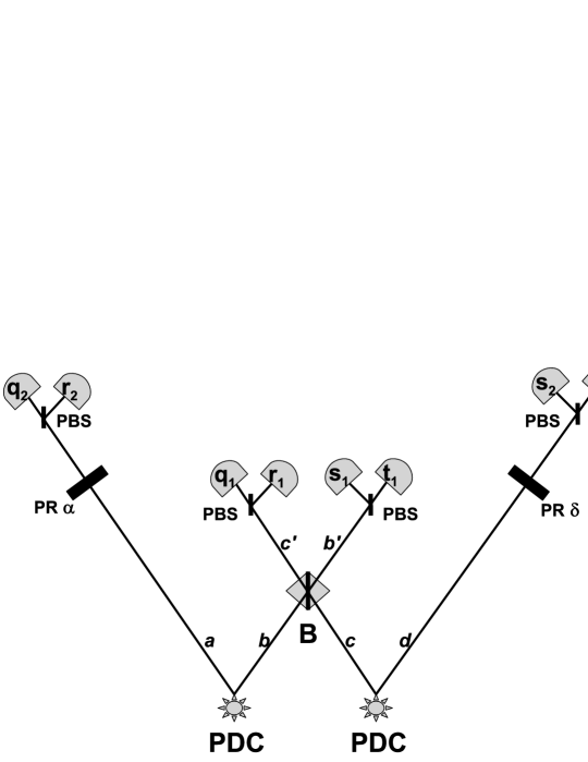
Figure 3: A scheme for entanglement verification in an entanglement swapping experiment. A Bell measurement with imperfect threshold detectors is performed on the $c$ and $b$ modes. A read-out $(q_{1}r_{1}s_{1}t_{1})$ is recorded. Polarization rotators (PR) parameterized by angles $\alpha$ and $\delta$ are applied to the remaining $a$ and $d$ modes prior to polarization measurements using polarizing beamsplitters (PBS) and non-ideal threshold detectors. The readout of the second measurement is denoted by $(q_{2}r_{2}s_{2}t_{2})$. For a fixed polarization rotation of the $a$ mode, $\alpha=\pi/4$, the observation of certain four-fold coincidences for varying rotation angles $0\leq\delta\leq\pi$ of the $d$ mode reveals, via the visibility $V$, the strength of the polarization correlations between the $a$ and $d$ modes.

In what follows, we provide the probability for four-fold coincidences using our model for practical entanglement swapping. Mathematically, the polarization rotators acting on the $a$ and $d$ modes are represented by the unitary operators

$$\hat{U}_{a}(\tilde{\alpha}) = \exp\left[i\tilde{\alpha}\hat{J}_{a}\right]\;,$$ (63)

$$\hat{U}_{d}(\tilde{\delta}) = \exp\left[i\tilde{\delta}\hat{J}_{d}\right]\;,$$ (64)

with $\tilde{\alpha},\tilde{\delta}\in\mathbb{R}$ and the generators of rotation

$$\hat{J}_{a} := \frac{1}{2}\left(\hat{a}_{\mbox{\tiny{V}}}^{\dagger}\hat{a}_{\mbox{\tiny{H}}}+\hat{a}_{\mbox{\tiny{V}}}\hat{a}_{\mbox{\tiny{H}}}^{\dagger}\right)\;,$$ (65)

$$\hat{J}_{d} := \frac{1}{2}\left(\hat{d}_{\mbox{\tiny{V}}}^{\dagger}\hat{d}_{\mbox{\tiny{H}}}+\hat{d}_{\mbox{\tiny{V}}}\hat{d}_{\mbox{\tiny{H}}}^{\dagger}\right)\;.$$ (66)

Here the angles $\tilde{\alpha}$ and $\tilde{\delta}$ are rotation angles of the Bloch vectors on the Bloch sphere and not of the polarization vectors in real space. As mentioned above, the former are related to the latter via $\tilde{\alpha}=2\alpha\;,\tilde{\delta}=2\delta$.

Given an event $(q_{1}r_{1}s_{1}t_{1})$ of an imperfect Bell measurement on modes $b$ and $c$, the conditional probability that polarization measurements on the $a$ and $d$ modes would have yielded the result $(i_{2}j_{2}k_{2}l_{2})$, if the detectors had been ideal, is given by

$$\mbox{prob}\left(i_{2}j_{2}k_{2}l_{2}|q_{1}r_{1}s_{1}t_{1}\right) = \mbox{Tr}\bigg{[}\left(|i^{a_{H}}_{2}j^{a_{V}}_{2}k^{d_{V}}_{2}l^{d_{H}}_{2}\rangle\langle i^{a_{H}}_{2}j^{a_{V}}_{2}k^{d_{V}}_{2}l^{d_{H}}_{2}|\right)\times\phantom{\bigg{]}}$$ (67)

$$\times\phantom{\bigg{[}}\left(\hat{U}_{a}(\tilde{\alpha})\otimes\hat{U}_{d}(\tilde{\delta}\,)\hat{\rho}^{q_{1}r_{1}s_{1}t_{1}}\hat{U}^{\dagger}_{a}(\tilde{\alpha})\otimes\hat{U}^{\dagger}_{d}(\tilde{\delta}\,)\right)\bigg{]}$$

$$= \sum_{i_{1}j_{1}k_{1}l_{1}}W^{i_{1}j_{1}k_{1}l_{1}}_{i_{2}j_{2}k_{2}l_{2}}(\tilde{\alpha},\tilde{\delta}\,)P^{q_{1}r_{1}s_{1}t_{1}}_{i_{1}j_{1}k_{1}l_{1}}(\,\chi,\{\eta^{(1)}_{\nu}\},\{{\wp^{(1)}_{\mbox{\tiny{dc}}\nu}}\})$$

where we have used Eq. (33) and introduced the transition probabilities

$$W^{i_{1}j_{1}k_{1}l_{1}}_{i_{2}j_{2}k_{2}l_{2}}(\tilde{\alpha},\tilde{\delta}\,) := \left|\langle i^{a_{H}}_{2}j^{a_{V}}_{2}k^{d_{V}}_{2}l^{d_{H}}_{2}|\hat{U}_{a}(\tilde{\alpha})\otimes\hat{U}_{d}(\tilde{\delta}\,)|\Phi_{i_{1}j_{1}k_{1}l_{1}}\rangle\right|^{2}\;.$$ (68)

The conditional probability to observe the event $(q_{2}r_{2}s_{2}t_{2})$ with non-ideal, imperfect detectors, given an event $(q_{1}r_{1}s_{1}t_{1})$ of a non-ideal Bell measurement on modes $b$ and $c$, is denoted and calculated as:

$$Q^{q_{1}r_{1}s_{1}t_{1}}_{q_{2}r_{2}s_{2}t_{2}}\left(\chi,\{\eta^{(1)}_{\nu}\},\{\eta^{(2)}_{\nu}\},\{{\wp^{(1)}_{\mbox{\tiny{dc}}\nu}}\},\{{\wp^{(2)}_{\mbox{\tiny{dc}}\nu}}\},\tilde{\alpha},\tilde{\delta}\right):=\mbox{prob}\left(q_{2}r_{2}s_{2}t_{2}|q_{1}r_{1}s_{1}t_{1}\right)$$

$$=\sum_{i_{2}j_{2}k_{2}l_{2}}\mbox{prob}(q_{2}r_{2}s_{2}t_{2}|i_{2}j_{2}k_{2}l_{2})\,\mbox{prob}(i_{2}j_{2}k_{2}l_{2}|q_{1}r_{1}s_{1}t_{1})$$

$$=\sum_{i_{2}j_{2}k_{2}l_{2}}p_{\eta_{1}^{(2)},\wp^{(2)}_{\mbox{\tiny{dc}}1}}(q_{2}|i_{2})\>p_{\eta_{2}^{(2)},\wp^{(2)}_{\mbox{\tiny{dc}}2}}(r_{2}|j_{2})\>p_{\eta_{3}^{(2)},\wp^{(2)}_{\mbox{\tiny{dc}}3}}(s_{2}|k_{2})\>p_{\eta_{4}^{(2)},\wp^{(2)}_{\mbox{\tiny{dc}}4}}(t_{2}|l_{2})\>\times$$

$$\times\left(\sum_{i_{1}j_{1}k_{1}l_{1}}W^{i_{1}j_{1}k_{1}l_{1}}_{i_{2}j_{2}k_{2}l_{2}}\big{(}\tilde{\alpha},\tilde{\delta}\,\big{)}P^{q_{1}r_{1}s_{1}t_{1}}_{i_{1}j_{1}k_{1}l_{1}}\big{(}\,\chi,\{\eta^{(1)}_{\nu}\},\{{\wp^{(1)}_{\mbox{\tiny{dc}}\nu}}\}\big{)}\right)$$

$$=\sum_{i_{2},j_{2},k_{2},l_{2}=0}^{\infty}\;\sum_{i_{1},j_{1},k_{1},l_{1}=0}^{\infty}p_{\eta_{1}^{(2)},\wp^{(2)}_{\mbox{\tiny{dc}}1}}(q_{2}|i_{2})\>p_{\eta_{2}^{(2)},\wp^{(2)}_{\mbox{\tiny{dc}}2}}(r_{2}|j_{2})\>p_{\eta_{3}^{(2)},\wp^{(2)}_{\mbox{\tiny{dc}}3}}(s_{2}|k_{2})\>p_{\eta_{4}^{(2)},\wp^{(2)}_{\mbox{\tiny{dc}}4}}(t_{2}|l_{2})\>$$

$$\hskip 85.35826pt\times W^{i_{1}j_{1}k_{1}l_{1}}_{i_{2}j_{2}k_{2}l_{2}}\big{(}\tilde{\alpha},\tilde{\delta}\,\big{)}P^{q_{1}r_{1}s_{1}t_{1}}_{i_{1}j_{1}k_{1}l_{1}}\big{(}\,\chi,\{\eta^{(1)}_{\nu}\},\{{\wp^{(1)}_{\mbox{\tiny{dc}}\nu}}\}\big{)}$$ (69)

For numerical simulations we need to know the transition probabilities (68). An explicit analytic expression is provided in the appendix C. This result together with Eqs. (55) and (47-49) enable us to calculate numerically the probabilities for four-fold coincidences. As explained above, we condition on obtaining the readout $(1_{c^{\prime}_{H}},0_{c^{\prime}_{V}},1_{b^{\prime}_{V}},0_{b^{\prime}_{H}})$ or $(0_{c^{\prime}_{H}},1_{c^{\prime}_{V}},0_{b^{\prime}_{V}},1_{b^{\prime}_{H}})$ in the Bell measurement. Given either of these two events occurs, regardless which of them, we calculate the conditional probabilities of recording the events $(1,0,1,0)$, $(0,1,1,0)$, $(0,1,0,1)$, and $(1,0,0,1)$, using the four-tuple $(D_{a}^{+},D_{a}^{-},D_{d}^{-},D_{d}^{+})$ of imperfect threshold detectors in the polarization measurement on the $a$ and $d$ modes, depending on the varying angle of rotation $\delta$.

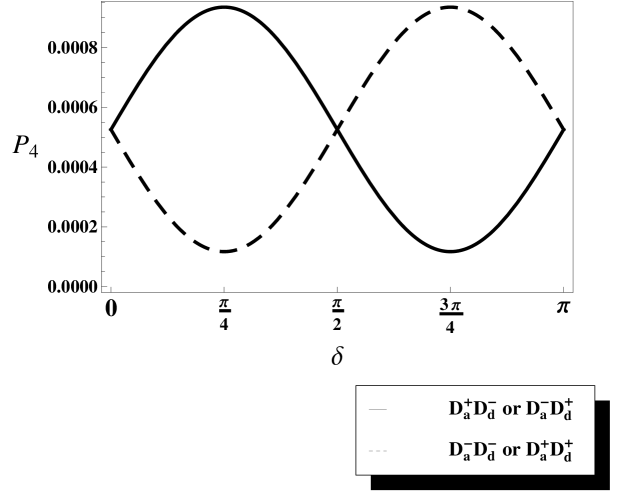
Figure 4: Simulated probability of four-fold coincidence $P_{4}$ depending on polarization rotation angle $\delta$, for a fixed rotation angle $\alpha=\pi/4$. Here $\alpha$ and $\delta$ represent angles of polarization rotations of the $a$ and $d$ modes in real space and not on the Bloch sphere. The experimental parameter values are given by $\chi\approx\sqrt{0,06}\approx 0.24$, $\eta^{(1)}_{1,2}=0.045$, $\eta^{(1)}_{3,4}=0.135$, $\eta^{(2)}_{1,2,3,4}=0.04$ and $\wp^{(1)}_{\mbox{\tiny{dc}}\,3,4}=1\times 10^{-5},\wp^{(1)}_{\mbox{\tiny{dc}}\,1,2}=\wp^{(2)}_{\mbox{\tiny{dc}}\,1,2,3,4}=3\times 10^{-5}$ in accordance with the conditions as found in the recent experiment RiedmattenMarcikicHouwelingenTittelZbindenGisin2005 . The continuous sinusoidal curve refers to the probability of the click coincidences “$D^{+}_{a}$ and $D^{-}_{d}$” or “$D^{-}_{a}$ and $D^{+}_{d}$” , and the dashed sinusoidal curve displays the probability of the click coincidences “$D^{-}_{a}$ and $D^{-}_{d}$” or “$D^{+}_{a}$ and $D^{+}_{d}$”, respectively, given that the Bell measurement yielded the result “$H$ and $V$” or “$V$ and $H$” for the $c$ and $b$ mode, respectively. The visibility is $V_{\mbox{\tiny th}}=77.7\%$.

In order to compare our predictions with experimental entanglement swapping, we have to choose the same experimental parameter values $\chi$, $\{\eta^{(1)}_{\nu}\}$, $\{\eta^{(2)}_{\nu}\}$, $\{{\wp^{(1)}_{\mbox{\tiny{dc}}\nu}}\}$, $\{{\wp^{(2)}_{\mbox{\tiny{dc}}\nu}}\}$ as in the experiment. It is important to emphasize that the detector efficiencies $\eta$ of our theory are to be considered as effective efficiencies that also include transmission and other losses, cf. Sec. II.3.2.

While we have developed our theory with entanglement swapping of polarization qubits as an intuitive example, it obviously also holds for any other realization of qubits, e.g. time-bin qubits TittelWeihs2001 . In the following we compare the predictions of our theory with a recent experiment on time-bin entanglement swapping RiedmattenMarcikicHouwelingenTittelZbindenGisin2005 , which explicitly mentions all required parameters related to the PDC sources, transmission line and detectors. Fig. 4 and Fig. 5 demonstrate results of our numerical simulations of four-fold coincidences with reference to experimental conditions of RiedmattenMarcikicHouwelingenTittelZbindenGisin2005 . The conditions of this experiment are given by the following approximate values: $\chi\approx\sqrt{0,06}\approx 0.24$, $\eta^{(1)}_{1,2}=0.045$, $\eta^{(1)}_{3,4}=0.135$, $\eta^{(2)}_{1,2,3,4}=0.04$ and $\wp^{(1)}_{\mbox{\tiny{dc}}\,3,4}=1\times 10^{-5},\wp^{(1)}_{\mbox{\tiny{dc}}\,1,2}=\wp^{(2)}_{\mbox{\tiny{dc}}\,1,2,3,4}=3\times 10^{-5}$. As expected, we get two complementary sine curves that are $90^{\circ}$ out of phase, one curve for anti-correlated polarization readouts (“$D^{+}_{a}$ and $D^{-}_{d}$” or “$D^{-}_{a}$ and $D^{+}_{d}$”) and another curve for correlated polarization readouts (“$D^{-}_{a}$ and $D^{-}_{d}$” or “$D^{+}_{a}$ and $D^{+}_{d}$”), at the detectors for the $a$ and $d$ modes. As anticipated, the probability to detect anti-correlated polarizations for the $a$ and $d$ modes attains its maximum for $\delta=\alpha=\pi/4$ and its minimum for $\delta=\alpha+\pi/2=3\pi/4$. Complementary to this, the probability to detect correlated polarizations has its maximum for $\delta=\alpha+\pi/2=3\pi/4$ and its minimum for $\delta=\alpha=\pi/4$. This is the characteristic entanglement property of the Bell state $|\Psi^{-}\rangle_{ad}$. The calculated visibility amounts to $V_{\mbox{\tiny th}}=77.7\%$. This is in respectably good agreement with the experimentally achieved visibility $V_{\mbox{\tiny exp}}=(80\pm 4)\%$ of RiedmattenMarcikicHouwelingenTittelZbindenGisin2005 .

Fig. 5 reveals the behavior of the visibility as a function of the square root of the photon-pair production rate $\chi$, for detector efficiencies and dark count probabilities chosen as given above. It is interesting to observe that the photon-pair production rate of the PDC sources used in this experiment, $\chi\approx 0.24$, lies far beyond its optimal value.

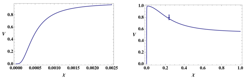
Figure 5: Visibility $V$ versus the square root of the photon-pair production rate $\chi$, for $\eta^{(1)}_{1,2}=0.045$, $\eta^{(1)}_{3,4}=0.135$, $\eta^{(2)}_{1,2,3,4}=0.04$ and $\wp^{(1)}_{\mbox{\tiny{dc}}\,3,4}=1\times 10^{-5},\wp^{(1)}_{\mbox{\tiny{dc}}\,1,2}=\wp^{(2)}_{\mbox{\tiny{dc}}\,1,2,3,4}=3\times 10^{-5}$. These values refer to the experimental situation of RiedmattenMarcikicHouwelingenTittelZbindenGisin2005 . The left image displays the functional dependence for very small $\chi$ values, the right image reveals the behavior for appreciably large values of $\chi$. For $\chi\approx 0.24$, which is the value found in the experiment RiedmattenMarcikicHouwelingenTittelZbindenGisin2005 , our numerical simulation (curve) yields the visibility $V_{\mbox{\tiny th}}=77.7\%$. The experimental result $V_{\mbox{\tiny exp}}=(80\pm 4)\%$ of RiedmattenMarcikicHouwelingenTittelZbindenGisin2005 is depicted by means of an $\pm 4\%$ error bar. A very good agreement is achieved. Our result also clearly demonstrates that the chosen photon-pair production rate belongs to a region with a rapidly decreasing visibility, thus being already far beyond its optimal value.

We have also compared the predictions of our model with the experimental data from the polarization entanglement swapping experiment reported in JenneweinWeihsPanZeilinger2002 . In this case, using $\chi$ =0.05 (which can be calculated from reported count rates, transmission loss and detector quantum efficiencies), we find $V_{\mbox{\tiny th}}=98\%$. Note that the experimentally obtained visibility, $V_{\mbox{\tiny exp}}\approx 90\%$, is much smaller than the value obtained from our model. This can easily be explained by taking into account that detector noise and multi-pair emissions are not the only practical limitations that impact on the visibility. Other deficiencies include imperfect entanglement created by each source, even in the case where only one single pair is generated, and imperfect temporal overlap of modes $b$ and $c$ on the beamsplitter that realizes the Bell state measurement. We believe the latter to be the main limitation in this experiment. Hence, our model currently only provides an upper, yet useful bound on the visibility.

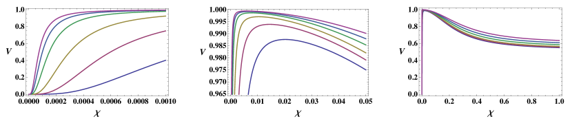
Figure 6: Visibility $V$ versus the square root of the photon-pair production rate $\chi$, for various detector efficiencies $\eta$ and the fixed dark count probability $\wp_{\mbox{\tiny{dc}}}=1\times 10^{-5}$. The function $V_{\eta,\wp_{\mbox{\tiny{dc}}}}(\chi)$ is plotted for six different efficiency values: $\eta=0.025,\>0.05,\>0.1,\>0.2,\>0.3,\>0.4$, corresponding to the curves of lowest to highest visibility in all three diagrams. The left diagram displays the dependence of the function $V_{\eta,\wp_{\mbox{\tiny{dc}}}}(\chi)$ on the parameter $\eta$ for very small $\chi$ values, the middle diagram shows the neighborhood of the maxima and the right diagram the behavior for high $\chi$ values. The regions displayed in the first two plots are also included in the third diagram where they correspond to the steep increase of the visibility for very small $\chi$ values.

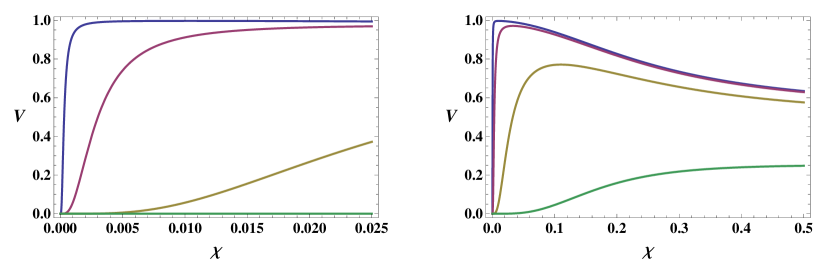
Figure 7: Visibility $V$ versus the square root of the photon-pair production rate $\chi$, for various detector dark count probabilities and the fixed efficiency $\eta=0.1$. Plots of the function $V_{\eta,\wp_{\mbox{\tiny{dc}}}}(\chi)$ are shown for four different detector dark count probabilities: $\wp_{\mbox{\tiny{dc}}}=1\times 10^{-2},\>1\times 10^{-3},\>1\times 10^{-4},\>1\times 10^{-5}$, corresponding to the curves of lowest to highest visibility in both diagrams. The left diagram displays the dependence of the function $V_{\eta,\wp_{\mbox{\tiny{dc}}}}(\chi)$ on the parameter $\wp_{\mbox{\tiny{dc}}}$ for small $\chi$ values, the right diagram the behavior for high $\chi$ values.

To analyze how entanglement is affected by detector imperfections, we have calculated the visibility $V_{\eta,\wp_{\mbox{\tiny{dc}}}}(\chi)$ as a function of $\chi$ for various detector efficiencies $\eta$ and dark count probabilities $\wp_{\mbox{\tiny{dc}}}$. To keep the analysis simple, we have assumed the same efficiencies and dark count probabilities for all detectors involved in the experimental setting. The dependence on $\eta$ and $\wp_{\mbox{\tiny{dc}}}$ is illustrated in Fig. 6 and Fig. 7. It is interesting to observe that, according to our theory, for reasonable low dark count probabilities ($\wp_{\mbox{\tiny{dc}}}\leq 10^{-4}$) there is a region of $\chi$-values such that the visibility can be made very close to $100\%$ even for low detector efficiencies. Given any detector efficiencies and dark counts, our model makes it possible to provide the optimal photon-pair production rate in order to achieve high entanglement after entanglement swapping. This is a valuable result. An important conclusion that can be drawn from our investigations is the feature that high photon-pair production rates are counter-productive. One should not exceed values of about $\chi=5\times 10^{-2}$. Higher $\chi$ values lead to a decreasing entanglement in the final quantum state after entanglement swapping and as such have an adverse impact. Yet, depending on the application, $V$ may not be the appropriate figure of merit to optimize.

First, in the here discussed proof-of-principle entanglement swapping experiments, the goal was to demonstrate a violation of the CHSH Bell inequality, rather than to maximize the violation. An important concern was thus to limit the time it took to take the data, generally many days. For the experiment RiedmattenMarcikicHouwelingenTittelZbindenGisin2005 we referred to in Fig. 5, this has resulted in source brightnesses $\chi$ exceeding the value required for maximum visibility.

As a second example where the visibility is not the relevant quantity to optimize, let us briefly consider QKD. Here, the figure of merit is the secret key rate, which scales in a non-trivial way with the visibility and with the number of detected coincidences Ma2007 . For the highest possible key rate, an optimal trade-off between the production rate of final entangled pairs, and visibility (i.e. amount of entanglement) has to be achieved. Hence, reducing the brightness of the PDC sources to a value that results in a maximum for $V$ does in general not lead to a maximum secret key rate.

IV Conclusion

Within the scope of our theory of practical entanglement swapping we have derived the actual quantum state of the remaining $a$ and $d$ modes depending on the result of a noisy Bell measurement with imperfect detectors and probabilistic sources. The main achievement consists in our ability to provide this quantum state for any given photon-pair production rate $\chi$, any given detector efficiency $\eta$ and any reasonable dark-count probability $\wp_{\mbox{\tiny{dc}}}$. In deriving our results we have made a distinction between photon-number discriminating detectors and threshold detectors. The calculated quantum state allows us to make predictions with regard to any quantity of interest. In particular, we can calculate the entanglement of the remaining modes, parameterized in terms of the visibility obtained in coincidence measurements, depending on the experimental parameters $\chi$, $\eta$ and $\wp_{\mbox{\tiny{dc}}}$.

Predictions of our theory have proved to be in close accord with experimental entanglement swapping. Our numerical simulations of certain four-fold coincidences between four threshold detectors demonstrate a remarkably good agreement with a recent entanglement swapping experiment reported in RiedmattenMarcikicHouwelingenTittelZbindenGisin2005 .

Furthermore, our theory provides a very useful functional relation between entanglement, quantified, e.g., by the visibility of four-fold coincidences, and the square root of the photon-pair production rate $\chi$. The latter is an essential experimental quantity in long-distance quantum key distribution based on protocols that employ quantum relays and repeater. The secret key rate, or equivalently the quantum bit error rate referred to as QBER, depend crucially on the photon-pair creation rate $\chi$. In our opinion, there sometimes is a tendency among scientists working on experimental QKD to aim at achieving brighter PDC sources due to the prevailed conception that higher photon-pair production rates lead to higher sifted-key rates. Here it should be realized, however, that it is not the source brightness itself that matters, but rather the production rate of final entangled photon-pairs after the swapping protocol, with their quantum correlations being as close as possible to that of Bell states. Our results indicate that in some experiments the optimal value of $\chi$ might eventually be exceeded. The investigations presented in section III suggest that, for a visibility of at least $97\%$, the photon-pair creation rates should not be chosen much greater than $\chi=0.05$. Higher values decrease the entanglement present after swapping, due to undesired multi-pair events from the same source, thus implying an increasing QBER. Hence, our results allow us to suggest the implications of the imperfections on schemes using entanglement swapping as a fundamental tool.

It should be emphasized, however, that, depending on the application, the amount of entanglement, as quantified by $V$, is not always the appropriate quantity to be made maximal. In QKD, for instance, the figure of merit is given by the secret key rate $R_{\mbox{\tiny sec}}$, and the non-trivial dependence of the latter on $\chi$ and the visibility $V$, cf. e.g. Ma2007 , suggests that the optimal $\chi$ values with respect to QKD are not necessarily those which yield the highest visibility of entanglement swapping. Nevertheless, we believe that the methods of the present work will prove very useful in finding the optimal photon-pair production rates with regard to achieving optimal secret-key rates in long distance, quantum repeater based QKD. As a first step into this direction we will have to generalize our results to several concatenated noisy entanglement swappings, and then examine the scaling properties with the number of these segments in the iteration.

In our future considerations we also plan to investigate the issue whether the optimal $\chi$ can be shifted to higher values by using photon-number discriminating detectors instead of threshold detectors for the Bell-state measurement. To understand the intuition, let us briefly discuss the events where a coincidence detection in two threshold detectors in modes $b^{\prime}$ and $c^{\prime}$ is interpreted as a projection onto a Bell state. For threshold detectors, a fraction of these cases originates from two photons impinging on one detector, and one photon impinging on the other detector. These undesired but not identifiable events result in a reduction of the swapped entanglement, i.e. visibility. Unit efficiency photon-number discriminating detectors would allow identifying and discarding these events, which leads to a higher visibility for equal source brightness, or, conversely, allows increasing the brightness while keeping the visibility constant. And so would do imperfect photon-number discriminating detectors to some extent. This conjecture is worth analyzing in view of promising technological advancements in research on photon-counting detectors Rosenberg2005A ; Rosenberg2005B . Obviously, though, if the PDC sources are too bright, events where only one click is detected at each output will be rare, and the production rate of final entangled pairs after the entanglement swapping operation will be low.

Acknowledgment: The authors acknowledge the support of NSERC, iCORE, CIFAR, MITACS, and General Dynamics Canada in preparing this work. We also thank Peter Marzlin and Thomas Jennewein for helpful discussions.

V Appendix

V.1 Dark count probability $\bm{\wp_{\mbox{\tiny{dc}}}}$

Throughout the paper we characterize dark counts in terms of the experimental parameter $\wp_{\mbox{\tiny{dc}}}$, which is defined to be the probability of a dark count event per detection window in a non-ideal threshold detector. Within our detector model, Eq. (23) provides $\wp_{\mbox{\tiny{dc}}}$ as a function of the parameter $\,r\,,$ or equivalently the pseudo temperature of the thermal source (22). To derive this relation, let us consider our detector model as depicted in Fig. 2 and at first assume the ideal photon-detector $D_{\mbox{\scriptsize id}}$ to be photon-number discriminating. Furthermore, we also suppose the signal mode to be in the vacuum state: $\hat{\rho}_{\mbox{\tiny sig}}=|\mbox{vac}\rangle\langle\mbox{vac}|$. Then, the probability of detecting $k$ dark count photons in the detector $D_{\mbox{\scriptsize id}}$ is obtained by applying the beam-splitter transformation $\hat{U}_{\mbox{\tiny BS}}(\eta)$ to the state $|\mbox{vac}\rangle\langle\mbox{vac}|\otimes\hat{\rho}_{\mbox{\tiny T}}$, followed by tracing over the reflected mode and projecting the transmitted mode onto the Fock state $|k\rangle$, and finally tracing over the latter mode. Hereby “reflection” and “transmission” refer to the signal mode. Thus, with the notation

$$\tilde{b}(\eta,r):=\eta\tanh^{2}r\;,$$ (70)

we have:

$$\mbox{prob}(\mbox{\it``k dark count photons"}) = \mbox{Tr}_{\mbox{\tiny trans}}\left[\hat{\Pi}_{k}\mbox{Tr}_{\mbox{\tiny refl}}\left[\hat{U}_{\mbox{\tiny BS}}(\eta)\left(|\mbox{vac}\rangle\langle\mbox{vac}|\otimes\hat{\rho}_{\mbox{\tiny T}}\right)\hat{U}^{\dagger}_{\mbox{\tiny BS}}(\eta)\right]\hat{\Pi}_{k}\right]\;$$ (71)

$$= \frac{1}{\cosh^{2}r}\sum_{n=k}^{\infty}{n\choose k}\left[\tanh^{2}r\right]^{n}\eta^{n-k}(1-\eta)^{k}\;$$

$$= \frac{1}{\cosh^{2}r}\left(\frac{1-\eta}{\eta}\right)^{k}\sum_{n=k}^{\infty}{n\choose k}\left[\tilde{b}(\eta,r)\right]^{n}$$

$$= \frac{1}{\cosh^{2}r}\left(\frac{1-\eta}{\eta}\right)^{k}\left[\tilde{b}(\eta,r)\right]^{k}\sum_{\nu=0}^{\infty}{\nu+k\choose k}\left[\tilde{b}(\eta,r)\right]^{\nu}\;,$$

where we used $\hat{\Pi}_{k}=|k\rangle\langle k|$ and the definition (22) of the thermal state $\hat{\rho}_{\mbox{\tiny T}}$. Since $0\leq\tilde{b}(\eta,r)<1$, we may apply the Lemma

$$\sum_{\nu=0}^{\infty}{\nu+k\choose k}q^{\nu}=\frac{1}{(1-q)^{k+1}}\quad\mbox{for}\quad 0\leq q<1\;,$$ (72)

which can be found in Stanley1999 . Hence,

$$\mbox{prob}(\mbox{\it``k dark count photons"})=\frac{1}{\cosh^{2}r}\left(\frac{1-\eta}{\eta}\right)^{k}\left[\frac{\tilde{b}(\eta,r)}{1-\tilde{b}(\eta,r)}\right]^{k}\frac{1}{1-\tilde{b}(\eta,r)}\;.$$ (73)

To obtain the probability for a dark count event in a photon-detector that does not discriminate between photon numbers, we have to sum over all integers $k\not=0$:

$$\wp_{\mbox{\tiny{dc}}} = \sum_{k=1}^{\infty}\mbox{prob}(\mbox{\it``k dark count photons"})$$ (74)

$$= \frac{1}{[1-\tilde{b}(\eta,r)]\cosh^{2}r}\sum_{k=1}^{\infty}\left[\frac{(1-\eta)\tilde{b}(\eta,r)}{\eta(1-\tilde{b}(\eta,r))}\right]^{k}\;.$$

Since

$$\theta:=\frac{(1-\eta)\tilde{b}(\eta,r)}{\eta[1-\tilde{b}(\eta,r)]}=\frac{(1-\eta)\tanh^{2}r}{1-\eta\tanh^{2}r}<1\;,$$ (75)

we finally get

$$\wp_{\mbox{\tiny{dc}}} = \frac{1}{\left[1-\tilde{b}(\eta,r)\right]\cosh^{2}r}\left(\sum_{k=0}^{\infty}\theta^{k}-1\right)$$ (76)

$$= \frac{1}{\left[1-\tilde{b}(\eta,r)\right]\cosh^{2}r}\left(\frac{1}{1-\theta}-1\right)$$

$$= \frac{(1-\eta)\tanh^{2}r}{1-\eta\tanh^{2}r}\;,$$

which is the result (23). Using this relation, we can express the function (70) in terms of $\eta$ and $\wp_{\mbox{\tiny{dc}}}$ rather than $\eta$ and $r$:

$$b(\eta,\wp_{\mbox{\tiny{dc}}}) := \tilde{b}\left(\eta,r(\eta,\wp_{\mbox{\tiny{dc}}})\right)$$ (77)

$$= \eta\tanh^{2}r=\left[1+\frac{1-\eta}{\eta\wp_{\mbox{\tiny{dc}}}}\right]^{-1}\;,$$

which is Eq. (26).

V.2 Conditional probabilities $\bm{p_{\eta,\wp_{\mbox{\tiny{dc}}}}(q|i)}$

The conditional probability $p_{\eta,\wp_{\mbox{\tiny{dc}}}}(q|i)$ to detect $q$ photons given that $i$ photons are incident upon a photon-number discriminating detector with efficiency $\eta$ and dark count probability $\wp_{\mbox{\tiny{dc}}}$ constitutes a major ingredient in our derivation of the quantum state after a realistic entanglement swapping operation. Here we derive its closed-form expression (25) using our detector model as depicted in Fig. 2. Assuming the signal mode to be in the Fock state $\hat{\rho}_{\mbox{\tiny sig}}=|i\rangle\langle i|$, according to Eq. (24) the conditional probability of interest is given as:

$$p_{\eta,\wp_{\mbox{\tiny{dc}}}}(q|i)=\mbox{Tr}_{\mbox{\tiny trans}}\left[\hat{\Pi}_{q}\mbox{Tr}_{\mbox{\tiny refl}}\left[\hat{U}_{\mbox{\tiny BS}}(\eta)\left(|i\rangle\langle i|\otimes\hat{\rho}_{\mbox{\tiny T}}\right)\hat{U}^{\dagger}_{\mbox{\tiny BS}}(\eta)\right]\hat{\Pi}_{q}\right]\;.$$ (78)

In what follows, we expand on the calculation of this expression. Using the relation (23), we expressed in (78) the dependence on the conditions of the thermal source in terms of the label $\wp_{\mbox{\tiny{dc}}}$ rather than the pseudo temperature of the source (or equivalently its parameter $r$). We will, however, initially use the notation $p_{\eta,r}(q|i)$ in the calculation below, and later show how the dark count probability $\wp_{\mbox{\tiny{dc}}}$ emerges in the final result.

Let $\hat{c},\;\hat{c}^{\dagger}$ and $\hat{e},\;\hat{e}^{\dagger}$ denote the annihilation and creation operators of the signal mode and the thermal mode (fictitious environment), respectively. Initially, their common quantum state, denoted by $\hat{\varrho}^{\mbox{\tiny in}}_{\mbox{\tiny sig,T}}$, is a product state, namely $\hat{\varrho}^{\mbox{\tiny in}}_{\mbox{\tiny sig,T}}=|i\rangle\langle i|\otimes\hat{\rho}_{\mbox{\tiny T}}$, where $\hat{\rho}_{\mbox{\tiny T}}$ is given by (22). We can express this input state as an operator functional of creation and annihilation operators:

$$\hat{\varrho}^{\mbox{\tiny in}}_{\mbox{\tiny sig,T}}=\hat{\varrho}^{\mbox{\tiny in}}_{\mbox{\tiny sig,T}}\left[\hat{c},\hat{c}^{\dagger},\hat{e},\hat{e}^{\dagger}\right]=\frac{1}{\cosh^{2}r}\sum_{n=0}^{\infty}\frac{\tanh^{2n}r}{i!n!}(\hat{c}^{\dagger})^{i}(\hat{e}^{\dagger})^{n}|\mbox{vac}\rangle\langle\mbox{vac}|\hat{e}^{n}\hat{c}^{i}\;.$$ (79)

Combining the signal with the thermal mode at a beamsplitter with transmittance $\eta$ leads to an entangled quantum state. In the Schrödinger picture, in which the photonic operators $\hat{c},\hat{c}^{\dagger},\hat{e},\hat{e}^{\dagger}$ remain unchanged, the beam-splitter transformation is represented by the unitary operator $\hat{U}_{\mbox{\tiny BS}}(\eta)$ which acts on input quantum states of the beamsplitter. Its action corresponds to replacing the creation and annihilation operators in the functional $\hat{\varrho}^{\mbox{\tiny in}}_{\mbox{\tiny sig,T}}\left[\hat{c},\hat{c}^{\dagger},\hat{e},\hat{e}^{\dagger}\right]$ by new operators according to the rule VogelWelsch2006 :

$${\hat{c}\choose\hat{e}}\rightarrow B_{\eta}^{\dagger}{\hat{c}\choose\hat{e}}\quad,\quad{\hat{c}^{\dagger}\choose\hat{e}^{\dagger}}\rightarrow B_{\eta}^{T}{\hat{c}^{\dagger}\choose\hat{e}^{\dagger}}\;,$$ (80)

where

$$B_{\eta}=\begin{pmatrix}\sqrt{\eta}&\sqrt{1-\eta}\\ -\sqrt{1-\eta}&\sqrt{\eta}\end{pmatrix}$$ (81)

is the beam-splitter transformation matrix consisting of the transmission and reflection coefficients $T=\sqrt{\eta}$ and $R=\sqrt{1-\eta}$. Applying the beam-splitter transformation yields the following entangled quantum state:

$$\hat{\varrho}^{\mbox{\tiny in}}_{\mbox{\tiny sig,T}}\stackrel{{\scriptstyle\mbox{\scriptsize BS}}}{{\longrightarrow}}\hat{\varrho}^{\mbox{\tiny out}}_{\mbox{\tiny sig,T}} := \hat{U}_{\mbox{\tiny BS}}(\eta)\hat{\varrho}^{\mbox{\tiny in}}_{\mbox{\tiny sig,T}}\hat{U}^{\dagger}_{\mbox{\tiny BS}}(\eta)$$ (82)

$$= \hat{U}_{\mbox{\tiny BS}}(\eta)\left(|i\rangle\langle i|\otimes\hat{\rho}_{\mbox{\tiny T}}\right)\hat{U}^{\dagger}_{\mbox{\tiny BS}}(\eta)$$

$$= \frac{1}{\cosh^{2}r}\sum_{n=0}^{\infty}\frac{\tanh^{2n}r}{i!\,n!}\left(\sqrt{\eta}\,\hat{c}^{\dagger}-\sqrt{1-\eta}\,\hat{e}^{\dagger}\right)^{i}\left(\sqrt{1-\eta}\,\hat{c}^{\dagger}+\sqrt{\eta}\,\hat{e}^{\dagger}\right)^{n}$$

$$\times\,|\mbox{vac}\rangle\langle\mbox{vac}|\left(\sqrt{1-\eta}\,\hat{c}+\sqrt{\eta}\,\hat{e}\right)^{n}\left(\sqrt{\eta}\,\hat{c}-\sqrt{1-\eta}\,\hat{e}\right)^{i}$$

$$= \frac{1}{\cosh^{2}r}\sum_{n=0}^{\infty}\frac{\tanh^{2n}r}{i!\,n!}\sum_{\nu=0}^{i}\sum_{\nu^{\prime}=0}^{i}\sum_{\mu=0}^{n}\sum_{\mu^{\prime}=0}^{n}{i\choose\nu}{i\choose\nu^{\prime}}{n\choose\mu}{n\choose\mu^{\prime}}$$

$$\times(-1)^{\nu+\nu^{\prime}}\left(\sqrt{\eta}\right)^{2n+\nu+\nu^{\prime}-\mu-\mu^{\prime}}\left(\sqrt{1-\eta}\right)^{2i-\nu-\nu^{\prime}+\mu+\mu^{\prime}}$$

$$\times\left(\hat{c}^{\dagger}\right)^{\nu+\mu}\left(\hat{e}^{\dagger}\right)^{i+n-\nu-\mu}|\mbox{vac}\rangle\langle\mbox{vac}|\hat{e}^{i+n-\nu^{\prime}-\mu^{\prime}}\hat{c}^{\nu^{\prime}+\mu^{\prime}}\;.$$

According to Eq. (78) the conditional probability $p_{\eta,r}(q|i)$ is obtained by ignoring the reflected mode and projecting the transmitted mode onto the Fock state $|q\rangle$, and finally taking the trace of the resultant non-normalized state. This can be rewritten as:

$$p_{\eta,r}(q|i)=\mbox{Tr}\left[\hat{\varrho}^{\mbox{\tiny out}}_{\mbox{\tiny sig,T}}\left(\hat{\Pi}_{q}^{\mbox{\tiny trans}}\otimes\openone^{\mbox{\tiny refl}}\right)\right]\;.$$ (83)

By inserting (82) into (83) and realizing that in the Schrödinger picture, which we use here, the mode $c$ in the equation (82) above corresponds to the transmitted and the mode $e$ to the reflected mode, respectively, we get:

$$p_{\eta,r}(q|i) = \frac{1}{\cosh^{2}r}\sum_{n=0}^{\infty}\frac{\tanh^{2n}r}{i!\,n!}\sum_{\nu=0}^{i}\sum_{\nu^{\prime}=0}^{i}\sum_{\mu=0}^{n}\sum_{\mu^{\prime}=0}^{n}{i\choose\nu}{i\choose\nu^{\prime}}{n\choose\mu}{n\choose\mu^{\prime}}$$ (84)

$$\times\,(-1)^{\nu+\nu^{\prime}}\left(\sqrt{\eta}\right)^{2n+\nu+\nu^{\prime}-\mu-\mu^{\prime}}\left(\sqrt{1-\eta}\right)^{2i-\nu-\nu^{\prime}+\mu+\mu^{\prime}}$$

$$\times\,\sqrt{(\nu+\mu)!}\sqrt{(\nu^{\prime}+\mu^{\prime})!}\sqrt{(i+n-\nu-\mu)!}\sqrt{(i+n-\nu^{\prime}-\mu^{\prime})!}$$

$$\times\,\delta_{q,\,\nu+\mu}\delta_{q,\;\nu^{\prime}+\mu^{\prime}}\delta_{i+n-\nu-\mu\,,\,i+n-\nu^{\prime}-\mu^{\prime}}\;$$

$$= \frac{1}{\cosh^{2}r}\sum_{n=0}^{\infty}\frac{\tanh^{2n}r}{i!\,n!}\sum_{\mu=0}^{n}\sum_{\mu^{\prime}=0}^{n}{i\choose q-\mu}{i\choose q-\mu^{\prime}}{n\choose\mu}{n\choose\mu^{\prime}}(-1)^{\mu+\mu^{\prime}}$$

$$\times\,\eta^{n+q}(1-\eta)^{i-q}\left(\frac{1-\eta}{\eta}\right)^{\mu+\mu^{\prime}}q!(i+n-q)!$$

$$= \frac{1}{\cosh^{2}r}\left(\frac{\eta}{1-\eta}\right)^{q}(1-\eta)^{i}\sum_{n=0}^{\infty}\left[\eta\tanh^{2}r\right]^{n}\frac{q!(i+n-q)!}{i!\,n!}\left[\Omega(\eta,i,q,n)\right]^{2}\;.$$

In the last step we have introduced the definition

$$\Omega(\eta,i,q,n):=\sum_{\mu=0}^{n}{i\choose q-\mu}{n\choose\mu}\left(\frac{\eta-1}{\eta}\right)^{\mu}\;.$$ (85)

It is important to recognize that $\Omega(\eta,i,q,n)=0$ unless $i\geq q-n$. This is intuitively understandable: the number $q$ of detected photons in $D_{\mbox{\scriptsize id}}$ cannot be greater than the sum $i+n$ of incident signal and thermal photons. To proceed, we have to distinguish two cases: $i\geq q$ and $i<q$. It is easily seen that in the case $i\geq q$ we have

$$\Omega(\eta,i,q,n)={i\choose q}\,_{2}F_{1}\left(-n,-q\,;i-q+1\,;\frac{\eta-1}{\eta}\right)\;,$$ (86)

where ${}_{2}F_{1}(\cdot,\cdot;\cdot;\cdot)$ is the Hypergeometric function as defined in (28). In the second case, $q>i$, we obtain:

$$\Omega(\eta,i,q,n) = \sum_{\mu=q-i}^{n}{i\choose q-\mu}{n\choose\mu}\left(\frac{\eta-1}{\eta}\right)^{\mu}$$ (87)

$$= \sum_{\kappa=0}^{n-q+i}{i\choose i-\kappa}{n\choose\kappa+q-i}\left(\frac{\eta-1}{\eta}\right)^{\kappa+q-i}$$

$$= \left(\frac{\eta-1}{\eta}\right)^{q-i}\;\sum_{\kappa=0}^{n-q+i}{i\choose\kappa}{n\choose n-q+i-\kappa}\left(\frac{\eta-1}{\eta}\right)^{\kappa}$$

$$= \left(\frac{\eta-1}{\eta}\right)^{q-i}{n\choose n-q+i}\sum_{\mu=0}^{n-q+i}{i\choose\mu}{n\choose n-q+i}^{-1}{n\choose n-q+i-\mu}\left(\frac{\eta-1}{\eta}\right)^{\mu}$$

$$= \left(\frac{\eta-1}{\eta}\right)^{q-i}{n\choose q-i}\;_{2}F_{1}\left(-i,q-i-n;q-i+1;\frac{\eta-1}{\eta}\right)\;.$$

We insert (86) into (84) and utilize the notation (70) to arrive at the following interim result for $i\geq q$:

$$p_{\eta,r}(q|i) = \frac{1}{\cosh^{2}r}\left(\frac{\eta}{1-\eta}\right)^{q}(1-\eta)^{i}\sum_{n=0}^{\infty}{i\choose q}{i-q+n\choose i-q}\left[\tilde{b}(\eta,r)\right]^{n}$$ (88)

$$\times\,\left[\,{}_{2}F_{1}\left(-n,-q\,;i-q+1\,;\frac{\eta-1}{\eta}\right)\right]^{2}\;.$$

For the $q>i$ case, we insert (87) into (84) and obtain:

$$p_{\eta,r}(q|i) = \frac{1}{\cosh^{2}r}\left(\frac{1-\eta}{\eta}\right)^{q-i}\eta^{i}\sum_{n=q-i}^{\infty}{q\choose i}{n\choose q-i}\left[\tilde{b}(\eta,r)\right]^{n}$$ (89)

$$\times\,\left[\,{}_{2}F_{1}\left(-i,q-i-n;q-i+1;\frac{\eta-1}{\eta}\right)\right]^{2}\;$$

$$= \frac{1}{\cosh^{2}r}\left(\frac{1-\eta}{\eta}\right)^{q-i}\eta^{i}\,\left[\tilde{b}(\eta,r)\right]^{q-i}\sum_{m=0}^{\infty}{q\choose i}{q-i+m\choose q-i}\left[\tilde{b}(\eta,r)\right]^{m}$$

$$\times\,\left[\,{}_{2}F_{1}\left(-i,-m\,;q-i+1\,;\frac{\eta-1}{\eta}\right)\right]^{2}\;$$

$$= \frac{1}{\cosh^{2}r}\left[\frac{1-\eta}{\eta}\,\tilde{b}(\eta,r)\right]^{q-i}\eta^{i}\sum_{n=0}^{\infty}{q\choose i}{q-i+n\choose q-i}\left[\tilde{b}(\eta,r)\right]^{n}$$

$$\times\,\left[\,{}_{2}F_{1}\left(-n,-i\,;q-i+1\,;\frac{\eta-1}{\eta}\right)\right]^{2}\;.$$

In the last step, after renaming the index of summation, $m\rightarrow n$, we made use of the permutation-symmetry property of Hypergeometric functions:

$${}_{2}F_{1}(\alpha,\beta;\gamma;z)=\,_{2}F_{1}(\beta,\alpha;\gamma;z)\;.$$ (90)

In this way a partial symmetry between the two results (88) and (89) is achieved. Please note that the result (89) is valid also for $q=i$, as in this case the right-hand side expressions of (88) and (89) coincide.

We would now like to replace the dependence on the parameter $r$ of the thermal source by a dependence on the dark count probability. The latter emerges in the following manner. We replace the function $\tilde{b}(\eta,r)$ by $b(\eta,\wp_{\mbox{\tiny{dc}}})$ according to Eq. (77) and use Eq. (23) to make the replacement

$$\frac{1}{\cosh^{2}r}=\frac{(1-\eta)(1-\wp_{\mbox{\tiny{dc}}})}{1-\eta(1-\wp_{\mbox{\tiny{dc}}})}\;.$$ (91)

Finally, by introducing the definition (27), we arrive at the result provided in Eq. (25).

V.3 Transition probabilities $\bm{W^{i_{1}j_{1}k_{1}l_{1}}_{i_{2}j_{2}k_{2}l_{2}}(\tilde{\alpha},\tilde{\delta})}$

In this appendix we provide an explicit analytic expression for the transition probabilities (68). Their definition involves unitary transformations representing polarization rotators for the $a$ and $d$ modes. According to Eqs. (63)-(66) the corresponding unitary operators are given by:

$$\hat{U}_{a}(\tilde{\alpha}) = \exp\left[i\frac{\tilde{\alpha}}{2}\left(\hat{a}_{\mbox{\tiny{V}}}^{\dagger}\hat{a}_{\mbox{\tiny{H}}}+\hat{a}_{\mbox{\tiny{V}}}\hat{a}_{\mbox{\tiny{H}}}^{\dagger}\right)\right]\;,$$ (92)

$$\hat{U}_{d}(\tilde{\delta}) = \exp\left[i\frac{\tilde{\delta}}{2}\left(\hat{d}_{\mbox{\tiny{V}}}^{\dagger}\hat{d}_{\mbox{\tiny{H}}}+\hat{d}_{\mbox{\tiny{V}}}\hat{d}_{\mbox{\tiny{H}}}^{\dagger}\right)\right]\;.$$ (93)

To find an explicit formula for $W^{i_{1}j_{1}k_{1}l_{1}}_{i_{2}j_{2}k_{2}l_{2}}(\tilde{\alpha},\tilde{\delta})$ it is very useful to “disentangle” these exponentials using a generalized Baker-Cambell-Hausdorf formula. Let us define

$$\hat{S}_{+}:=\hat{a}_{\mbox{\tiny{V}}}^{\dagger}\hat{a}_{\mbox{\tiny{H}}}\;,\quad\hat{S}_{-}:=\hat{a}_{\mbox{\tiny{V}}}\hat{a}_{\mbox{\tiny{H}}}^{\dagger}\;,\quad\hat{S}_{z}:=\frac{1}{2}\left(\hat{a}_{\mbox{\tiny{V}}}^{\dagger}\hat{a}_{\mbox{\tiny{V}}}-\hat{a}_{\mbox{\tiny{H}}}^{\dagger}\hat{a}_{\mbox{\tiny{H}}}\right)\;.$$ (94)

These operators form a bosonic representation of the su(2) Lie algebra, as they obey the commutation relations of generators of the latter. According to Ban1993 ; PuriBook , the following decomposition formula holds for exponential functions of the generators of the su(2) Lie algebra:

$$\exp\left[i\tilde{\alpha}\left(\theta_{+}\hat{S}_{+}+\theta_{z}\hat{S}_{z}+\theta_{-}\hat{S}_{-}\right)\right]=\exp\left(f_{+}(\tilde{\alpha})\hat{S}_{+}\right)\exp\left(f_{z}(\tilde{\alpha})\hat{S}_{z}\right)\exp\left(f_{-}(\tilde{\alpha})\hat{S}_{-}\right)$$ (95)

where the functions $f_{\pm}(\tilde{\alpha}),f_{z}(\tilde{\alpha})$ are given by:

$$f_{\pm}(\tilde{\alpha}) := \frac{i\theta_{\pm}}{\Gamma_{1}}\frac{\sin(\Gamma_{1}\tilde{\alpha})}{\cos(\Gamma_{1}\tilde{\alpha})-i\theta_{z}\sin(\Gamma_{1}\tilde{\alpha})/(2\Gamma_{1})}\;,$$ (96)

$$f_{z}(\tilde{\alpha}) := -2\ln\left[\cos(\Gamma_{1}\tilde{\alpha})-i\frac{\theta_{z}}{2\Gamma_{1}}\sin(\Gamma_{1}\tilde{\alpha})\right]\;,$$ (97)

with

$$\Gamma_{1}^{2}:=\theta_{+}\theta_{-}+\frac{\theta_{z}^{2}}{4}\;.$$ (98)

We apply this decomposition formula to Eq. (92). In our case we have $\theta_{+}=\theta_{-}=1/2$ and $\theta_{z}=0$, yielding $\Gamma_{1}=1/2\;$ and

$$f_{\pm}(\tilde{\alpha}) = i\tan\frac{\tilde{\alpha}}{2}\;,$$ (99)

$$f_{z}(\tilde{\alpha}) = -2\ln\left(\cos\frac{\tilde{\alpha}}{2}\right)\;.$$ (100)

Thus, Eq. (92) becomes:

$$\hat{U}_{a}(\tilde{\alpha}) = \exp\left[i\tan\left(\frac{\tilde{\alpha}}{2}\right)\hat{a}_{\mbox{\tiny{V}}}^{\dagger}\hat{a}_{\mbox{\tiny{H}}}\right]\exp\left[-\ln\left(\cos\frac{\tilde{\alpha}}{2}\right)\hat{a}_{\mbox{\tiny{V}}}^{\dagger}\hat{a}_{\mbox{\tiny{V}}}\right]$$ (101)

$$\times\exp\left[\ln\left(\cos\frac{\tilde{\alpha}}{2}\right)\hat{a}_{\mbox{\tiny{H}}}^{\dagger}\hat{a}_{\mbox{\tiny{H}}}\right]\exp\left[i\tan\left(\frac{\tilde{\alpha}}{2}\right)\hat{a}_{\mbox{\tiny{V}}}\hat{a}_{\mbox{\tiny{H}}}^{\dagger}\right]\;.$$

In a similar way we obtain a decomposition of $\hat{U}_{d}(\tilde{\delta})$ in Eq. (93). The result reads:

$$\hat{U}_{d}(\tilde{\delta}) = \exp\left[i\tan\left(\frac{\tilde{\delta}}{2}\right)\hat{d}_{\mbox{\tiny{V}}}^{\dagger}\hat{d}_{\mbox{\tiny{H}}}\right]\exp\left[-\ln\left(\cos\frac{\tilde{\delta}}{2}\right)\hat{d}_{\mbox{\tiny{V}}}^{\dagger}\hat{d}_{\mbox{\tiny{V}}}\right]$$ (102)

$$\times\exp\left[\ln\left(\cos\frac{\tilde{\delta}}{2}\right)\hat{d}_{\mbox{\tiny{H}}}^{\dagger}\hat{d}_{\mbox{\tiny{H}}}\right]\exp\left[i\tan\left(\frac{\tilde{\delta}}{2}\right)\hat{d}_{\mbox{\tiny{V}}}\hat{d}_{\mbox{\tiny{H}}}^{\dagger}\right]\;.$$

We use these expressions in (68) to derive the transition probabilities. A straightforward but lengthy calculation yields the following result:

$$W^{i_{1}j_{1}k_{1}l_{1}}_{i_{2}j_{2}k_{2}l_{2}}(\tilde{\alpha},\tilde{\delta}\,)=\left|A^{i_{1}j_{1}k_{1}l_{1}}_{i_{2}j_{2}k_{2}l_{2}}(\tilde{\alpha},\tilde{\delta}\,)\right|^{2}$$ (103)

with

$$A^{i_{1}j_{1}k_{1}l_{1}}_{i_{2}j_{2}k_{2}l_{2}}(\tilde{\alpha},\tilde{\delta}\,) := \langle i^{a_{H}}_{2}j^{a_{V}}_{2}k^{d_{V}}_{2}l^{d_{H}}_{2}|\hat{U}_{a}(\tilde{\alpha})\otimes\hat{U}_{d}(\tilde{\delta})|\Phi_{i_{1}j_{1}k_{1}l_{1}}\rangle$$

$$= \frac{1}{(\sqrt{2})^{i_{1}+j_{1}+k_{1}+l_{1}}\sqrt{i_{1}!j_{1}!k_{1}!l_{1}!}}\sum_{\mu=0}^{i_{1}}\sum_{\nu=0}^{j_{1}}\sum_{\kappa=0}^{k_{1}}\sum_{\lambda=0}^{l_{1}}(-1)^{\mu+\nu}{i_{1}\choose\mu}{j_{1}\choose\nu}{k_{1}\choose\kappa}{l_{1}\choose\lambda}$$

$$\times\delta_{\mu+\nu+\kappa+\lambda\,,\,i_{2}+j_{2}}\,\delta_{i_{1}+j_{1}+k_{1}+l_{1}\,,\,i_{2}+j_{2}+k_{2}+l_{2}}$$

$$\times\sqrt{(\mu+\lambda)!(\nu+\kappa)!(i_{1}+l_{1}-\mu-\lambda)!(j_{1}+k_{1}-\nu-\kappa)!}$$

$$\times\sum_{n_{a}=0}^{\mbox{\scriptsize min}\{j_{2},\nu+\kappa\}}\;\sum_{n_{d}=0}^{\mbox{\scriptsize min}\{k_{2},j_{1}+k_{1}-\nu-\kappa\}}\left[\cos\frac{\tilde{\alpha}}{2}\right]^{i_{2}+j_{2}-2n_{a}}\left[\cos\frac{\tilde{\delta}}{2}\right]^{k_{2}+l_{2}-2n_{d}}$$

$$\times\left\{\frac{\left[i\tan\frac{\tilde{\alpha}}{2}\right]^{j_{2}+\nu+\kappa-2n_{a}}\left[i\tan\frac{\tilde{\delta}}{2}\right]^{k_{2}+j_{1}+k_{1}-\nu-\kappa-2n_{d}}}{(j_{2}-n_{a})!(\nu+\kappa-n_{a})!(k_{2}-n_{d})!(j_{1}+k_{1}-\nu-\kappa-n_{d})!}\right\}$$

$$\times\left[\prod_{m_{1}=1}^{j_{2}-n_{a}}(n_{a}+m_{1})\right]^{\frac{1}{2}}\left[\prod_{m_{2}=1}^{\nu+\kappa-n_{a}}(n_{a}+m_{2})\right]^{\frac{1}{2}}$$

$$\times\left[\prod_{m_{3}=1}^{j_{2}-n_{a}}(i_{2}+m_{3})\right]^{\frac{1}{2}}\left[\prod_{m_{4}=1}^{\nu+\kappa-n_{a}}(i_{2}+j_{2}-\nu-\kappa+m_{4})\right]^{\frac{1}{2}}$$

$$\times\left[\prod_{m_{5}=1}^{k_{2}-n_{d}}(n_{d}+m_{5})\right]^{\frac{1}{2}}\left[\prod_{m_{6}=1}^{j_{1}+k_{1}-\nu-\kappa-n_{d}}(n_{d}+m_{6})\right]^{\frac{1}{2}}$$

$$\times\left[\prod_{m_{7}=1}^{k_{2}-n_{d}}(l_{2}+m_{7})\right]^{\frac{1}{2}}\left[\prod_{m_{8}=1}^{j_{1}+k_{1}-\nu-\kappa-n_{d}}(k_{2}+l_{2}-j_{1}-k_{1}+\nu+\kappa+m_{8})\right]^{\frac{1}{2}}$$

References

• (1) H. J. Briegel, W. Dür, J. I. Cirac, and P. Zoller, Phys. Rev. Lett. 81, 5932 (1998).
• (2) L.-M. Duan, M. D. Lukin, J. I. Cirac, and P. Zoller, Nature 414, 413 (2001).
• (3) N. Gisin, G. Ribordy, W. Tittel and H. Zbinden, Rev. Mod. Phys. 74, 145 (2002).
• (4) E. Waks, A. Zeevi and Y. Yamamoto, Phys. Rev. A 65, 052310 (2002).
• (5) B. C. Jacobs, T. B. Pittman and D. Franson, Phys. Rev. A 66, 052307 (2002).
• (6) H. de Riedmatten, I. Marcikic, W. Tittel, H. Zbinden, D. Collins, and N. Gisin, Phys. Rev. Lett. 92, 047904 (2004).
• (7) D. Collins, N. Gisin and H. de Riedmatten, J. Mod. Opt. 52, 735 (2005).
• (8) M. $\dot{\mbox{Z}}$ukowski, A. Zeilinger, M. A. Horne and A. K. Ekert, Phys. Rev. Lett. 71, 4287 (1993).
• (9) G. Brassard, N. Lütkenhaus, T. Mor and B. C. Sanders, Phys. Rev. Lett. 85, 1330 (2000).
• (10) C. H. Bennett and G. Brassard, in Proceedings of IEEE International Conference on Computers, Systems and Signal Processing, Bangalore, India (IEEE, New York, 1984), p. 175.
• (11) A. K. Ekert, J. G. Rarity, P. R. Tapster, and G. M. Palma, Phys. Rev. Lett. 69, 1293 (1992).
• (12) A. V. Sergienko, M. Atatüre, Z. Walton, G. Jaeger, B. E. A. Saleh, and M. C. Teich, Phys. Rev. A 60, R2622 (1999).
• (13) X. Ma, C.-H. F. Fung, and H.-K. Lo, Phys. Rev. A 76, 012307 (2007).
• (14) I. Marcikic, H. de Riedmatten, W. Tittel, V. Scarani, H. Zbinden, and N. Gisin, Phys. Rev. A 66, 062308 (2002).
• (15) H. de Riedmatten, V. Scarani, I. Marcikic, A. Acín, W. Tittel, H. Zbinden, and N. Gisin, J. Mod. Opt. 51, 1637 (2004).
• (16) J. B. Brask and A. S. Sørensen, Phys. Rev. A 78, 012350 (2008).
• (17) L. Jiang, J. M. Taylor, and M. D. Lukin, Phys. Rev. A 76, 012301 (2007).
• (18) B. Zhao, Z.-B. Chen, Y.-A. Chen, J. Schmiedmayer, and J.-W. Pan, Phys. Rev. Lett. 98, 240502 (2007).
• (19) Ş. K. Özdemir, A. Miranowicz, M. Koashi, and N. Imoto, Phys. Rev. A 66, 053809 (2002).
• (20) P. P. Rohde and T. C. Ralph, Phys. Rev. A 73, 062312 (2006).
• (21) X. Jia, X. Su, Q. Pan, C. Xie, and K. Peng, J. Opt. B: Quantum Semiclass. Opt. 7, 189-193 (2005).
• (22) W. Tittel and G. Weihs, Quantum Inf. Comput. 1, 3 (2001).
• (23) H. Weinfurter, Europhys. Lett. 25, 559 (1994).
• (24) M. Michler, K. Mattle, H. Weinfurter and A. Zeilinger, Phys. Rev. A 53, R1209 (1996).
• (25) S. D. Bartlett, D. A. Rice, B. C. Sanders, J. Daboul and H. de Guise, Phys. Rev. A 63, 042310 (2001).
• (26) F. Bussières, J.  A. Slater, N. Godbout, and W. Tittel, Opt. Express 16, 17060 (2008).
• (27) M. Ban, J. Opt. Soc. Am. B 10, 1347 (1993).
• (28) R. R. Puri, Mathematical Methods of Quantum Optics (Springer, Berlin and Heidelberg, 2001).
• (29) S. D. Barlett and B. C. Sanders, Phys. Rev. A. 65, 042304 (2002).
• (30) P. P. Rohde and T.C. Ralph, J. Mod. Op. 53, 1589 (2006).
• (31) J. Appel, D. Hoffman, E. Figueroa, and A. I. Lvovsky, Phys. Rev.  A 75, 035802 (2007).
• (32) D. Rosenberg, A. E. Lita, A. J. Miller, S. W. Nam and R. E. Schwall, IEEE Trans. Appl. Supraconductivity 15(2), 575 (2005).
• (33) D. Rosenberg, A. E. Lita, A. J. Miller and S. W. Nam, Phys. Rev. A. 71, 061803 (2005).
• (34) J. von Neumann, Mathematische Grundlagen der Quantenmechanik (Springer, Berlin, 1932).
• (35) W. Vogel and D.-G. Welsch, Quantum Optics (WILEY-VCH Verlag, Weinheim, 2006).
• (36) J.-W. Pan, D. Bouwmeester, H. Weinfurter and A. Zeilinger, Phys. Rev. Lett. 80, 3891 (1998).
• (37) T. Jennewein, G. Weihs, J. W. Pan and A. Zeilinger, Phys. Rev. Lett. 88, 017903 (2002).
• (38) H. de Riedmatten, I. Marcikic, J. A. W. van Houwelingen, W. Tittel, H. Zbinden and N. Gisin, Phys. Rev. A. 71, 050302 (2005).
• (39) J. F. Clauser, M. A. Horne, A. Shimony, and R. A. Holt, Phys. Rev. Lett. 23, 880 (1969).
• (40) I. Marcikic, H. de Riedmatten, W. Tittel, H. Zbinden, N. Gisin, Nature 421, 509 (2003).
• (41) J. G. Rarity and P. R. Tapster, Phys. Rev. Lett. 64, 2495 (1990).
• (42) H. de Riedmatten, I. Marcikic, W. Tittel, H. Zbinden, and N. Gisin, Phys. Rev. A 67, 022301 (2003).
• (43) R. P. Stanley, Enumerative Combinatorics:Volume 1 (Cambridge University Press, Cambridge, 1999).