Spin dynamics and structure formation in a spin-1 condensate in a magnetic field

Abstract

We study the dynamics of a trapped spin-1 condensate in a magnetic field. First, we analyze the homogeneous system, for which the dynamics can be understood in terms of orbits in phase space. We analytically solve for the dynamical evolution of the populations of the various Zeeman components of the homogeneous system. This result is then applied via a local density approximation to trapped quasi-1D condensates. Our analysis of the trapped system in a magnetic field shows that both the mean-field and Zeeman regimes are simultaneously realized, and we argue that the border between these two regions is where spin domains and phase defects are generated. We propose a method to experimentally tune the position of this border.

I Introduction

Bose-Einstein condensates (BECs) with a spin degree of freedom are an interesting field of research in many-body physics as they realize both superfluidity and magnetism in a well-controlled environment. First realized experimentally with ²³Na ten years ago Stamper-Kurn et al. (1998); Stenger et al. (1998), their study has matured remarkably over the last few years, with several groups studying their dynamics Chang et al. (2004); Schmaljohann et al. (2004a); Kronjäger et al. (2005); Higbie et al. (2005) and thermodynamics Erhard et al. (2004); Schmaljohann et al. (2004b). Of particular interest is the study of the process by which spin domains are formed during time evolution, a phenomenon observed experimentally Chang et al. (2005); Higbie et al. (2005); Sadler et al. (2006) and in numerical simulations based on a mean-field approach Mur-Petit et al. (2006); Saito and Ueda (2005); Zhang et al. (2005a).

The complicated dynamics of these non-linear systems, especially when they are subjected to time-varying external fields, makes the physical understanding of the structure formation process somehow elusive. To address this point, we present here a simple model based on an analytic solution for the homogeneous system for arbitrary magnetic fields $B$ and magnetizations ${\cal M}$. This solution is then applied to the study of realistic, trapped spin-1 condensates by means of the local density approximation (LDA). This approximation has already been applied successfully in a number of studies on scalar BECs, as well as cold Fermi gases. From the analysis of our results we are able to provide an intuitive picture of the process leading to the structure formation. Further, we argue that it should be possible to experimentally “tune” the spatial region where this process starts within the condensate.

The paper is organized as follows. In Sect. II.1 we present the phase space of a homogeneous system under a magnetic field $B$ and for arbitrary ${\cal M}$, and introduce the phase-space orbits that describe the dynamics of a conservative system. In Sect. II.2 we solve analytically the dynamical evolution of the homogeneous system. Then, in Sect. III we describe our local-density approximation for a trapped system and present numerical results for its dynamics (Sect. III.1), which we compare with simulations based on a mean-field treatment (Sect. III.3). In Sect. IV we discuss the progressive dephasing of different spatial points of the condensate in a homogeneous magnetic field, and relate this to the process of structure formation, with an indication of a possible experimental test. Finally, we conclude in Sect. V.

II Analytical results for the homogeneous system

II.1 Energetics of the homogeneous system

A homogeneous condensate of atoms with total spin $F$ can be described by a vector order parameter $\vec{\psi}$ with $2F+1$ components,

$$\vec{\psi} =\left(\begin{array}[]{c}\psi_{F}\\ \vdots\\ \psi_{-F}\end{array}\right)\>.$$ (4)

The density of atoms in a given Zeeman component $m=-F,\cdots,F$ is $n_{m}=|\psi_{m}|^{2}$ and the total density is given by $n=\sum_{m}|\psi_{m}|^{2}$. Introducing the relative densities for the homogeneous system $\lambda_{m}=n_{m}/n$, one has

$$\sum_{m}\lambda_{m}=1\>.$$ (5)

Given that $n$ is a conserved quantity, Eq. (5) will be fulfilled at all times during the dynamical evolution. Moreover, the magnetization

$${\cal M}=\sum_{m}m\lambda_{m}$$ (6)

is also a conserved quantity Mur-Petit et al. (2006).

We now focus our analysis to the case of a $F=1$ condensate. We write the various components of the order parameter as $\psi_{m}=\sqrt{n\lambda_{m}}\exp(i\theta_{m})$. This ansatz, together with conditions (5) and (6), leads to the following expression for the energy per particle of the homogeneous system in the mean-field approach Moreno-Cardoner et al. (2007); Zhang et al. (2003):

$${\cal E}(\lambda_{0}, {\cal M},\theta)=c_{2}n\Big{[}\lambda_{0}(1-\lambda_{0})+\frac{{\cal M}^{2}}{2}+$$

$$+\lambda_{0}\sqrt{(1-\lambda_{0})^{2}-{\cal M}^{2}}\cos\theta\Big{]}+\delta(1-\lambda_{0})\>.$$ (7)

Here $\theta=2\theta_{0}-\theta_{1}-\theta_{-1}$, while $c_{2}$ is given in terms of the $s$-wave scattering lengths $a_{f}$ in the channels of total spin $f=0,2$, by $c_{2}=4\pi\hbar^{2}(a_{2}-a_{0})/(3M)$, with $M$ as the atomic mass. Finally, $\delta=(E_{-}+E_{+}-2E_{0})/2$, where the energies of the atomic Zeeman states are given by the Breit-Rabi formula Breit and Rabi (1931) $E_{m}=-E_{\mathrm{hfs}}/8-E_{\mathrm{hfs}}\sqrt{1+m\alpha+\alpha^{2}}/2$ ($m=-1,0,+1$), with $E_{\textrm{hfs}}$ being the atomic hyperfine splitting and $\alpha=(g_{I}\mu_{N}+g_{J}\mu_{B})B/E_{\textrm{hfs}}$ is a function of the external magnetic field $B$. Here, $g_{I},g_{J}$ are the nuclear and electronic Landé factors, and $\mu_{N},\mu_{B}$ are the nuclear and Bohr magnetons, respectively. A sketch of the surface ${\cal E}$ is given in Fig. 1.

Figure 1: Energy (in units of $|c_{2}|n$) of the homogeneous system for the cases (a) ${\cal M}=0,\leavevmode\nobreak\ B=0$ and (b) ${\cal M}=0.3,\leavevmode\nobreak\ B=1$ mG, as given by Eq. (7) for a spin-1 condensate of ⁸⁷Rb.

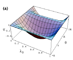
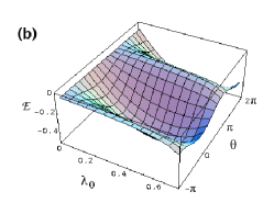
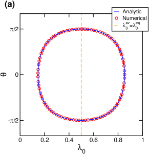
As indicated above, ${\cal M}$ is a constant during dynamical evolution. Similarly, given initial conditions $(\lambda_{0}^{\mathrm{in}},\theta_{\mathrm{in}})$, $E={\cal E}(\lambda_{0}^{\mathrm{in}},{\cal M},\theta_{\mathrm{in}})$ will also be conserved, thus defining an orbit on the surface ${\cal E}$ in $(\lambda_{0},\theta)$ space. A sketch of one such orbit is presented in Fig. 2.

Figure 2: Contour plot of the energy surface corresponding to ${\cal M}=0.3$ and $B=100$ mG. The white line shows the orbit corresponding to the initial conditions $\lambda_{0}^{\mathrm{in}}=1/2,\leavevmode\nobreak\ \theta_{\mathrm{in}}=\pi/2$ (indicated by the white dot). The minimum of $\cal E$ is at $\lambda_{0}\approx 0.455,\leavevmode\nobreak\ \theta=0$. Note the presence of open orbits for energies above that of the indicated white line.

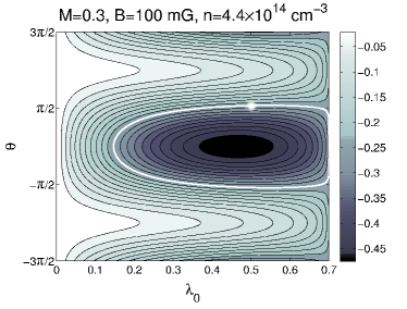
One should note that, depending on the initial conditions, the orbit defined by $E=\textrm{const}$ can be closed or open. In the first case, $\theta=\theta(t)$ will be a periodic function of time, while in the latter case, $|\theta(t)|$ will grow indefinitely with time. In both cases, however, $\lambda_{0}=\lambda_{0}(t)$ will be a periodic function of time.

II.2 Dynamics of the homogeneous system

We are interested in the time evolution of the densities of the different Zeeman components, $n_{m}=n\lambda_{m}$. From Eqs. (5) and (6) we have that

$$\lambda_{\pm 1} =\frac{1\pm{\cal M}-\lambda_{0}}{2}\>.$$ (8)

Therefore, we only need to follow the evolution of $\lambda_{0}$, which is given by

$$\frac{\partial\lambda_{0}}{\partial t}\equiv\dot{\lambda_{0}}=\frac{2}{\hbar}c_{2}n\lambda_{0}\sqrt{(1-\lambda_{0})^{2}-{\cal M}^{2}}\sin\theta\>.$$ (9)

With Eq (7), we rewrite this as

$$(\dot{\lambda_{0}})^{2}=\frac{4}{\hbar^{2}}\bigg{\{}(c_{2}n\lambda_{0})^{2}\left[(1-\lambda_{0})^{2}-{\cal M}^{2}\right]$$

$$-\left[E-\delta(1-\lambda_{0})-c_{2}n\left(\lambda_{0}(1-\lambda_{0})+\frac{{\cal M}^{2}}{2}\right)\right]^{2}\bigg{\}}\>.$$

It can be shown that the term in $\lambda_{0}^{4}$ actually drops out and we are left with a cubic polynomial on $\lambda_{0}$,

$$(\dot{\lambda_{0}})^{2} \equiv A(\lambda_{0}-\Lambda_{1})(\lambda_{0}-\Lambda_{2})(\lambda_{0}-\Lambda_{3})\>,$$ (10)

with

$$A:=-\frac{8c_{2}n\delta}{\hbar^{2}}\>,$$ (11)

and $\Lambda_{j}\leavevmode\nobreak\ (j=1,2,3)$ are the roots of $(\dot{\lambda_{0}})^{2}$, $\Lambda_{1}<\Lambda_{2}<\Lambda_{3}$. For ground state ($F=1$) alkalies $\delta>0$. Therefore, $\Lambda_{1}\leq\lambda_{0}(t)\leq\Lambda_{2}$ for $c_{2}<0$ and $\Lambda_{2}\leq\lambda_{0}(t)\leq\Lambda_{3}$ for $c_{2}>0$ Zhang et al. (2005b). For concreteness, in the following we will assume $c_{2}\leq 0$, i.e., ferromagnetic interactions.

We will now integrate the time evolution of $\lambda_{0}$. To do so, we introduce an auxiliary variable $z$ through $\lambda_{0}=(\Lambda_{2}-\Lambda_{1})z^{2}+\Lambda_{1}$. This will satisfy the differential equation

$$\dot{z}=\frac{\sqrt{A}}{2}\sqrt{\Lambda_{2}-\Lambda_{1}}\sqrt{(z^{2}-1)(z^{2}-k^{-2})}$$ (12)

where we defined

$$k^{2}:=\frac{\Lambda_{2}-\Lambda_{1}}{\Lambda_{3}-\Lambda_{1}}\in[0,1]\>.$$ (13)

The first order differential equation (12) can be solved analytically by separating the variables $z$ and $t$, and integrating:

$$\frac{\sqrt{A}}{2}\int_{t_{0}}^{t}dt =\frac{1}{\sqrt{\Lambda_{2}-\Lambda_{1}}}\int_{z_{0}}^{z_{t}}\frac{dz}{\sqrt{(1-z^{2})(k^{-2}-z^{2})}}=$$

$$=\frac{1}{\sqrt{\Lambda_{3}-\Lambda_{1}}}\int_{z_{0}}^{z_{t}}\frac{dz}{\sqrt{(1-z^{2})(1-k^{2}z^{2})}}\>.$$

The solution to the last integral can be expressed in terms of the elliptic integral of the first kind ,

$$F(\phi,k)=\int_{0}^{\sin\phi}\frac{dz}{\sqrt{(1-z^{2})(1-k^{2}z^{2})}}\>.$$

Taking as initial condition $z(t=t_{0})=z_{0}$ and using the fact that $F(-u,k)=-F(u,k)$, we can express $z_{t}$ in a compact form by means of the Jacobi elliptic functions Abramowitz and Stegun (1972), which are defined as the inverses of the elliptic integrals,

$$z_{t}\equiv z(t)=\textrm{sn}\Big{(}\gamma_{0}+\frac{\sqrt{A(\Lambda_{3}-\Lambda_{1})}}{2}(t-t_{0})\leavevmode\nobreak\ \Big{|}\leavevmode\nobreak\ k\Big{)}$$ (14)

with $z_{0}=\textrm{sn}(\gamma_{0}|k)$, i.e., $\gamma_{0}:=F(\arcsin(z_{0}),k)$. Finally, we undo the change in variables to write down the time evolution of the population of the $|m=0\rangle$ state,

$$\lambda_{0} (t)=\Lambda_{1}+$$

$$(\Lambda_{2}-\Lambda_{1})\,\textrm{sn}^{2}\!\left(\gamma_{0}+\frac{\sqrt{A(\Lambda_{3}-\Lambda_{1})}}{2}(t-t_{0})\leavevmode\nobreak\ \Big{|}k\right).$$ (15)

In accordance with the identity Abramowitz and Stegun (1972)

$$\textrm{sn}^{2}(\alpha|k)=\frac{1-\textrm{cn}(2\alpha|k)}{1+\textrm{dn}(2\alpha|k)}\>,$$

and given that both $\textrm{cn}(2\alpha|k)$ and $\textrm{dn}(2\alpha|k)$ are periodic functions in $\alpha$ with period $2K(k)$, $\lambda_{0}(t)$ will be a periodic function of time with period

$$T=\frac{2\hbar}{\sqrt{-2c_{2}n\delta(\Lambda_{3}-\Lambda_{1})}}\,K\left(\sqrt{\frac{\Lambda_{2}-\Lambda_{1}}{\Lambda_{3}-\Lambda_{1}}}\right)\>.$$ (16)

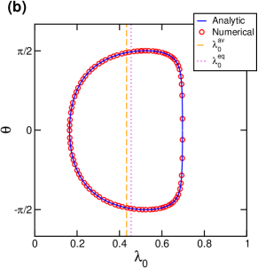
Here, $K(k)=F(\pi/2,k)$ stands for the complete elliptic integral of the first kind. We note that result (16) agrees with that in Ref. Zhang et al. (2005b), where $T$ was calculated directly by performing the integral $T=\oint d\lambda_{0}/\dot{\lambda_{0}}$ over a period of evolution. Further, let us point out that the average value $\lambda_{0}^{\textrm{av}}=(1/T)\int_{t_{0}}^{t_{0}+T}\lambda_{0}(t)\,dt$ does not necessarily coincide with the position of the minimum of $\cal E$, i.e., $\lambda_{0}^{\textrm{av}}$ may differ from the equilibrium value $\lambda_{0}^{\mathrm{eq}}$ (as given, e.g., in Ref. Moreno-Cardoner et al. (2007) for the case $B=0$). This is illustrated in Figs. 3(b) and 4(b).

II.3 Evolution in the absence of a magnetic field

We observe that the representation of $(\dot{\lambda_{0}})^{2}$ as a cubic polynomial on $\lambda_{0}$, Eq. (10), cannot be performed when $A=0$, i.e., when $B=0$. In this case, the analytic expression (15) is meaningless, as it would apparently result in no time evolution at all. Actually, in this situation, $(\dot{\lambda_{0}})^{2}$ can be written as a quadratic polynomial on $\lambda_{0}$:

$$(\dot{\lambda_{0}})^{2} =-\frac{4}{\hbar^{2}}\left\{2c_{2}nE\lambda_{0}^{2}-2c_{2}nE^{\prime}\lambda_{0}+(E^{\prime})^{2}\right\}$$

$$\equiv\overline{A}(\lambda_{0}-\overline{\Lambda}_{1})(\lambda_{0}-\overline{\Lambda}_{2})$$ (17)

$$\overline{\Lambda}_{1,2} =\frac{E^{\prime}}{2E}\left[1\mp\sqrt{1-\frac{2E}{c_{2}n}}\right]\qquad(\overline{\Lambda}_{1}<\overline{\Lambda}_{2})\>.$$ (18)

Here $E^{\prime}=E-c_{2}n{\cal M}^{2}/2$. Note that $\overline{A}:=-8c_{2}nE/\hbar^{2}\propto-c_{2}^{2}<0$ for $c_{2}<0$ as well as for $c_{2}>0$, and in both cases we will have $\overline{\Lambda}_{1}\leq\lambda_{0}(t)\leq\overline{\Lambda}_{2}$. Following a procedure analogous to that above, we arrive at

$$\lambda_{0}(t)=\overline{\Lambda}_{1}+(\overline{\Lambda}_{2}-\overline{\Lambda}_{1})\sin^{2}\!\left(\overline{\gamma}_{0}-\frac{\pi}{T_{B=0}}(t-t_{0})\right)$$ (19)

with $\sin\overline{\gamma}_{0}=\left[(\lambda_{0}^{\mathrm{in}}-\overline{\Lambda}_{1})/(\overline{\Lambda}_{2}-\overline{\Lambda}_{1})\right]^{1/2}$. In this case, $\lambda_{0}$ follows a pure sinusoidal evolution as has been predicted before in a number of references, e.g., Moreno-Cardoner et al. (2007); Zhang et al. (2005b); Pu et al. (1999). The average value is $\lambda_{0}^{\textrm{av}}=(\overline{\Lambda}_{1}+\overline{\Lambda}_{2})/2=E^{\prime}/(2E)$, and the period reads (compare with Pu et al. (1999))

$$T_{B=0}=\frac{\pi\hbar}{\sqrt{2c_{2}nE}}\>.$$ (20)

We show in Fig. 3 the time evolution of $\lambda_{0}(t)$ for two representative cases. The different panels compare the analytic evolution –given by Eq. (15) or (19)– with a numerical solution of the corresponding equation for $\dot{\lambda_{0}}$. In all cases, we see that the amplitude as well as the period of the time evolution are well predicted by the analytic results.

Figure 3: Evolution of the population of the $m=0$ Zeeman component, $\lambda_{0}(t)$, for the cases (a) ${\cal M}=0,\leavevmode\nobreak\ B=0$, and (b) ${\cal M}=0.3,\leavevmode\nobreak\ B=100$ mG, starting in both instances from $\lambda_{0}^{\mathrm{in}}=0.5,\leavevmode\nobreak\ \theta_{\mathrm{in}}=\pi/2$. In both panels, the solid line corresponds to the analytic result, (a) Eq. (19) or (b) (15), while the circles are a numerical integration of the differential equation for $\dot{\lambda_{0}}$. The dashed line gives the expected average value of $\lambda_{0}$, $\lambda_{0}^{\textrm{av}}\approx 0.433$. The arrows indicate the amplitude and period as predicted by the analytical results. In the bottom plot, also the value of the equilibrium population $\lambda_{0}^{\mathrm{eq}}\approx 0.455$ is indicated by a dotted line, while the dashed-dotted line stands for a fit to Eq. (26) (displaced vertically by 0.1 for clarity).

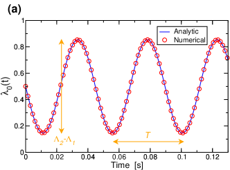
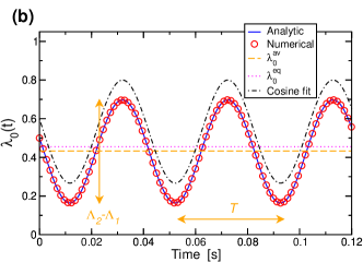
Finally, we show in Fig. 4 a plot of $\theta(t)$ vs. $\lambda_{0}(t)$ corresponding to the time evolution depicted in Fig. 3. For the case with magnetic field and ${\cal M}\neq 0$ we observe that the average value $\lambda_{0}^{\textrm{av}}\approx 0.433$ (indicated by the dashed line) differs from the position of the minimum of $\cal E$ ($\lambda_{0}^{\mathrm{eq}}\approx 0.455$, cf. Fig. 2) due to the deformation of the orbit.

Figure 4: Phase-space plot $(\lambda_{0},\theta)$ corresponding to (a) the evolution shown in Fig. 3(a) and (b) Fig. 3(b) (compare with Fig. 2). The solid line is the analytic result in (a) Eq. (19) and (b) Eq. (15), while the circles are the solution of the differential equations for $\dot{\lambda_{0}}$ and $\dot{\theta}$. The vertical dashed lines stand for the average value $\lambda_{0}^{\textrm{av}}$ in each case.

III Dynamics of the trapped system

We have established in the previous section the dynamical evolution of a homogeneous spin-1 condensate, in terms of orbits in the $(\lambda_{0},\theta)$ plane constrained by (i) conservation of density, (ii), conservation of magnetization, and (iii) conservation of energy. The resulting dynamics of the population of the $|m=0\rangle$ Zeeman component has been shown to be a periodic function of time, with a period determined by the density $n$ of the system, its magnetization ${\cal M}$, as well as the initial conditions of the evolution (implicit in $E$ and, therefore, in $\{\Lambda_{j}\}_{j=1,2,3}$ or $\{\overline{\Lambda}_{j}\}_{j=1,2}$), cf. Eqs. (16) and (20). Now, we will transfer these results to a realistic case of a trapped, quasi-one-dimensional (1D) condensate.

III.1 Local-density approximation

The initial conditions for the evolution of a trapped spinor condensate are the set of complex values $\psi_{m}^{\textrm{in}}(\bm{x})$ for all Zeeman components $m$ and all positions $\bm{x}$ where the density is not zero. In typical experiments, the preparation of the initial state is such that $n_{m}(\bm{x})/n(\bm{x})$ is a constant independent of position. This, together with the fact that $|c_{2}|\ll|c_{0}|$ for the systems studied so far, has lead to some theoretical works based on the so-called single-mode approximation (SMA), which assumes that $n_{m}(\bm{x},t)=n(\bm{x})\lambda_{m}(t)$ for all times $t$ of the evolution, i.e., that the spatial variation in the density of each Zeeman component is always given by the total density profile. However, numerical studies beyond the SMA (e.g., Mur-Petit et al. (2006); Pu et al. (1999); Saito and Ueda (2005)) predicted the formation of spin domains as time goes by. These have been observed in a number of experiments, e.g., Stenger et al. (1998); Higbie et al. (2005). In order to be able to observe the formation of spin domains during time evolution in a trapped system, we will therefore not make use of the SMA, but apply the analytical results of Sect. II via the LDA, i.e., we will assume that the evolution of the $|m=0\rangle$ population at each point within the condensate, $\lambda_{0}(\bm{x},t)$, is given by Eq. (15) [or Eq. (19)] with the substitution $n\rightarrow n(\bm{x})$. Here, the total density is normalized to the total number of atoms in the condensate, $\int d\bm{x}\,n(\bm{x})=N$. Similarly, we introduce the local densities of atoms in a given Zeeman state $n_{m}(\bm{x},t)$ normalized as $\int d\bm{x}\,n_{m}(\bm{x},t)=N_{m}(t)$. The conservation laws read now $\sum_{m}N_{m}(t)=N$ and $\sum_{m}mN_{m}(t)={\cal M}$. We note that $n(\bm{x})$ does not change in time at low enough temperatures Mur-Petit et al. (2006) unless momentum is imparted to the center of mass or to one or more of the Zeeman components Guilleumas et al. (2008).

In the language of the phase space introduced in Sect. II.1, a trapped system corresponds to an infinite-dimensional phase space, with a pair of variables $(\lambda_{0}(\bm{x}),\theta(\bm{x}))$ associated to each point $\bm{x}$. According to the LDA, we divide this whole phase space in sections corresponding to the different positions, and assume that they are independent. The initial condition described above, $n_{m}(\bm{x})/n(\bm{x})=\textrm{const}$, corresponds then to the dynamical system starting in all the different positions $\bm{x}$ at the same point of the corresponding phase space, $(\lambda_{0}(\bm{x},t=0)=\lambda_{0}^{\mathrm{in}},\leavevmode\nobreak\ \theta(\bm{x},t=0)=\theta_{\mathrm{in}})$. The dynamical evolution of the system corresponds then to the population $\lambda_{0}(\bm{x},t)$ at each point $\bm{x}$ following its own particular orbit in the corresponding $(\lambda_{0}(\bm{x}),\theta(\bm{x}))$ space, that is, $\lambda_{0}$ at position $\bm{x}$ follows the dynamical equation of the homogeneous system (15) [or Eq. (19)] with the parameters $\Lambda_{j}$ and $A$ determined by the local density $n(\bm{x})$. In other words, we assume that the position dependence is only parametric, and comes through the values of the parameters $\Lambda_{j}=\Lambda_{j}(\bm{x})$ and $T=T(\bm{x})$. We will indicate this by $\lambda_{0}(\bm{x},t)=\lambda_{0}^{\textrm{LDA}}(\bm{x},t)\equiv\lambda_{0}^{n(\bm{x})}(t)$. The density at position $\bm{x}$ of atoms in the Zeeman component $m$ at time $t$ will then be

$$n_{m}(\bm{x},t)=n(\bm{x})\lambda_{m}(\bm{x},t)\>.$$ (21)

with $\lambda_{\pm 1}(\bm{x},t)=\lambda_{\pm 1}^{n(\bm{x})}(t)$ given by Eq. (8) with the substitution $\lambda_{0}\rightarrow\lambda_{0}^{n(\bm{x})}(t)$, and ${\cal M}={\cal M}(t=0)$ is a conserved quantity Mur-Petit et al. (2006).

Note that the orbits associated to different points $\bm{x}$ may differ from one another, as their shapes depend inter alia on the local density $n(\bm{x})$, cf. Eq. (7). This fact, together with the position dependence of the parameters $\Lambda_{j}(\bm{x})$ and $T(\bm{x})$, is expected to lead to a dephasing of the evolution of the partial densities $n_{m}(\bm{x},t)$ at the different points, washing out the oscillations in the integrated populations, $N_{m}(t)$, in contrast to the stable oscillations that we have found for the homogeneous system, cf. Fig. 3.

In order to evaluate $N_{m}(t)$ it is necessary to know the density profile of the system. A good estimate for $n(\bm{x})$ in trapped atomic gases is given by the Thomas-Fermi approximation,

$$n_{\textrm{TF}}(\bm{x}) =\left\{\begin{array}[]{ll}\frac{n_{\textrm{max}}}{R_{\textrm{TF}}^{2}}(R_{\mathrm{TF}}^{2}-|\bm{x}|^{2})\>,&\quad|\bm{x}|\leq R_{\mathrm{TF}}\\ 0\>,&\quad\textrm{otherwise}\end{array}\right.\>.$$ (24)

For a quasi-1D system with total number of atoms $N$ and central density $n_{\mathrm{max}}$, $R_{\mathrm{TF}}=3N/(4n_{\mathrm{max}})$. The integrated population in $|m=0\rangle$ then reads

$$N_{0}(t)=\int dx\,n_{\textrm{TF}}(x)\lambda_{0}^{n_{\textrm{TF}}(x)}(t)\>.$$ (25)

III.2 Analytic approximation with sinusoidal time dependence

The time dependence of $\lambda_{0}^{n(x)}(t)$ has in principle to be calculated from Eq. (15) for each position $x$ at each time step, and then the integral (25) performed numerically to determine $N_{0}(t)$. It is possible however to give an analytical estimation for $N_{0}(t)$ if we make a further assumption on the time evolution. From Fig. 3, we see that the evolution of $\lambda_{0}(t)$ for the homogeneous system is very close to a sinusoidal function even when $B\neq 0$ . This is illustrated in Fig. 3(b), where a function of the form

$$\lambda_{0}^{\textrm{cos}}(t)=a+b\cos(\gamma+\nu t)$$ (26)

has been fitted to the numerical values obtained from Eq. (15). The fit is very good, even for this case, where the orbit in phase space is strongly deformed [cf. Fig. 4(b)]. The advantage of approximating the time evolution of $\lambda_{0}$ by Eq. (26) is that it allows for an analytic evaluation of the spatial integral (25), taking into account the position dependence of $\nu$. Indeed, from Eq. (16) we expect $\nu(x)\propto n(x)\propto(R_{\mathrm{TF}}^{2}-x^{2})$. It is easy to show that

$$N_{0}^{\textrm{cos}}(t) =\int dx\,n_{\textrm{TF}}(x)\left[a+b\cos\!\left[\gamma+\nu_{0}(1-\frac{x^{2}}{R_{\mathrm{TF}}^{2}})t\right]\right]$$

$$=\frac{n_{\textrm{max}}}{6(\nu_{0}t)^{3/2}}\Big{[}8a(\nu_{0}t)^{3/2}+6b\sqrt{\nu_{0}t}\sin(2\gamma)$$

$$+3\sqrt{2\pi}b\left\{\cos(\mu)S(\eta)-\sin(\mu)C(\eta)\right\}$$

$$+6\sqrt{2\pi}b\nu_{0}t\left\{\cos(\mu)C(\eta)+\sin(\mu)S(\eta)\right\}\Big{]}.$$ (27)

Here $S(\eta)$ and $C(\eta)$ are the Fresnel integrals Abramowitz and Stegun (1972), and we introduced $\mu=\gamma+\nu_{0}t$ and $\eta=\sqrt{2\nu_{0}t/\pi}$.

We show in Fig. 5 the time evolution of the integrated $|m=0\rangle$ population as given by Eqs. (25) and (27).

Figure 5: Time evolution of the integrated $|m=0\rangle$ population (normalized to the total population, $N=20\,000$) for $\lambda_{0}^{\mathrm{in}}=0.5,\leavevmode\nobreak\ \theta_{\mathrm{in}}=\pi/2,\leavevmode\nobreak\ {\cal M}=0.3$ and $B=100$ mG. The solid line shows the LDA result, Eq. (25), with $\lambda_{0}(x,t)=\lambda_{0}^{n(x)}(t)$. The circles stand for the analytic estimate of Eq. (27), and the dashed line is the result of integrating the set of coupled Gross-Pitaevskii equations (29).

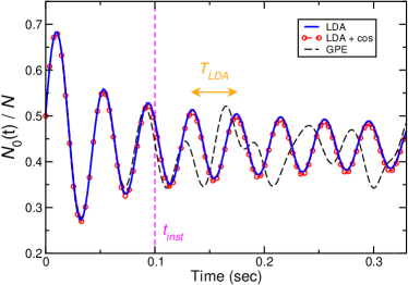
This calculation has been done for a quasi-1D system of $20\,000$ ⁸⁷Rb atoms in a trap such that the central density is $4.4\times 10^{14}$ cm^-3. The initial conditions are $\lambda_{0}^{\mathrm{in}}=0.5,\leavevmode\nobreak\ \theta_{\mathrm{in}}=\pi/2$ and ${\cal M}=0.3$ and we have taken a magnetic field $B=100$ mG (cf. Fig. 2). The solid line in the figure corresponds to the numerical integration of Eq. (25) with $\lambda_{0}(x,t)=\lambda_{0}^{n(x)}(t)$ given by Eq. (15). The circles stand for the analytic expression (27) with the parameters $a,b,\gamma,\nu_{0}$ taken so that $\lambda_{0}^{\textrm{cos}}(t)$ for a homogeneous system with density $n=n_{\mathrm{max}}$ reproduces the same behavior as that given by Eq. (15) at the same density: $a=(\Lambda_{1}+\Lambda_{2})/2,\leavevmode\nobreak\ b=(\Lambda_{1}-\Lambda_{2})/2,\leavevmode\nobreak\ \gamma=2\gamma_{0},\leavevmode\nobreak\ \nu_{0}=2\pi/T_{\textrm{LDA}}$, and $T_{\textrm{LDA}}=T(n_{\mathrm{max}})$. The agreement between the two calculations is very good at all times. Therefore, we conclude that the average value of $\lambda_{0}$ as well as the characteristic period of the oscillations is well determined by the values $\Lambda_{j}$ and $T_{\textrm{LDA}}$ calculated with the central density, while the time scale for the damping of the oscillations is determined by the spatial profile of the density.

Regarding the dephasing of the evolution of $\lambda_{0}(\bm{x},t)$ among different points, it is not very strong, in the sense that the damping of the oscillations is relatively slow. To be more precise, one can have a reasonable fit to the solid line in Fig. 5 by a function of the form

$$N_{0}(t)=\overline{N}_{0}+\Delta N_{0}\exp(-\alpha\sqrt{t})\cos\left(2\gamma_{0}^{\prime}+\frac{2\pi}{T^{\prime}}t\right)$$ (28)

with $\overline{N}_{0}\approx a$, $\Delta N_{0}\approx b$, $\gamma_{0}^{\prime}\approx\gamma_{0}$ and $T^{\prime}\approx T_{\textrm{LDA}}$.

III.3 Comparison with the mean-field approach

We proceed finally to compare the approximate calculation of $N_{0}(t)$ with a more complete approach in terms of the dynamical equations for the three components of the vector order parameter, $\psi_{m}(\bm{x},t)$, cf. Eq. (4). In the mean-field approximation, such equations can be cast in the form of three coupled Gross-Pitaevskii equations Mur-Petit et al. (2006),

$$i\hbar\frac{\partial\psi_{\pm 1}}{\partial t}= [{\cal H}_{s}+c_{2}(n_{\pm 1}+n_{0}-n_{\mp 1})]\psi_{\pm 1}+c_{2}\psi_{0}^{2}\psi^{*}_{\mp 1}\,,$$ (29a)

$$i\hbar\frac{\partial\psi_{0}}{\partial t}= [{\cal H}_{s}+c_{2}(n_{1}+n_{-1})]\psi_{0}+2c_{2}\psi_{1}\psi_{0}^{*}\psi_{-1}\,,$$ (29b)

where ${\cal H}_{s}=-\hbar^{2}/(2M)\,{\bm{\nabla}}^{2}+V_{\textrm{ext}}(\bm{x})+c_{0}n(\bm{x})$ and $c_{0}=4\pi\hbar^{2}(a_{0}+2a_{2})/(3M)$.

The results of solving Eqs. (29) with a Runge-Kutta algorithm are included in Fig. 5 as a dashed line. The average value of the oscillating $\lambda_{0}(t)$ is well estimated by the analytical model of Sect. II.2. Also, the characteristic time scale of the oscillations is well estimated by Eq. (16). The overall agreement is good for times $t\lesssim 100$ ms. After this time, the analytical estimate keeps oscillating with a slowly decreasing amplitude, while the numerical solution of the coupled equations (29) shows fluctuating oscillations. This behavior has been observed before, and the transition at $t=t_{\textrm{inst}}\sim 100$ ms has been related to a dynamical instability that leads to the formation of dynamical spin domains in the system Saito and Ueda (2005); Mur-Petit et al. (2006); Higbie et al. (2005). It is thus not surprising that our simple model fails for $t\gtrsim t_{\textrm{inst}}$. It is nevertheless remarkable that the time scale set by $T_{\textrm{LDA}}=T(n_{\mathrm{max}})\approx 89$ ms is still a good estimate of the characteristic oscillation time even much later during the time evolution.

IV Dephasing in a magnetic field and the process of structure formation in finite systems

A qualitative difference between the homogeneous system and the confined one appears when a magnetic field is present and, therefore, $A\neq 0$. The dynamics of a spinor condensate in a magnetic field is known to show two limiting behaviors: the mean-field regime, where the interaction energy dominates the evolution, and the Zeeman regime, where the evolution is driven by the Zeeman term of the Hamiltonian Zhang et al. (2005b); Sadler et al. (2006); Kronjäger et al. (2006). The crossover between the two regimes occurs when $c_{2}n\sim\delta$. This transition can be studied in real time by changing the (homogeneous) magnetic field on which the condensate is immersed Sadler et al. (2006); Saito et al. (2007); Mur-Petit et al. .

This transition can also be observed between different spatial regions of an inhomogeneous system. Indeed, if we assume that the magnetic field, magnetization and central density are chosen so that $|c_{2}|n(x=0)>\delta$ (so that at the center we are in the mean-field regime), then at the wings of the system, where $n(x)\rightarrow 0$, we will be in the Zeeman regime. Therefore, we expect to have a region in real space where the behavior with time changes qualitatively. For a profile as in Eq. (24), this transition border is given by

$$\frac{x_{\textrm{trans}}}{R_{\mathrm{TF}}}=\textrm{Re}\left[1-\frac{\delta}{c_{2}n_{\mathrm{max}}}\right]^{1/2}\>.$$ (30)

Naturally, for $\delta=0$, there is no transition (the density vanishes at $x=R_{\mathrm{TF}}$). On the other hand, for large enough magnetic field the whole system is in the Zeeman regime ($x_{\textrm{trans}}=0$).

These two regimes evolve with different characteristic times, $T_{\textrm{mf}}\simeq\hbar/(|c_{2}|n)$ and $T_{\textrm{Zeeman}}\simeq\hbar/\sqrt{2c_{2}n\delta}$, cf. Eqs. (20) and (16). Because of this, we can expect $\lambda_{0}$ and the phase in the inner part of the condensate ($|x|<x_{\textrm{trans}}$) to evolve at a different rate than in the outer wings of the system ($|x|>x_{\text{trans}}$), resulting in a particular spatial dependence of the phase. We note that the appearance of a spatial structure in the phase will lead to the creation of spin currents Mur-Petit et al. (2006) and, thus, to spin textures as reported in Chang et al. (2005); Sadler et al. (2006). Even though a smooth density profile will lead to a smooth variation in $T(x)=T(n(x))$ with position, from our model we expect that these qualitatively different behaviors should be observable for times $t\gtrsim t_{\textrm{trans}}=\textrm{min}\{T_{\textrm{mf}},T_{\textrm{Zeeman}}\}$

Interestingly, in light of the discussion in Sect. III.3, we observe that the time when the dynamical instability is expected to set in is close to the time when the divergence between mean-field and Zeeman regimes should be observable: $t_{\textrm{inst}}\simeq t_{\textrm{trans}}$. Because processes such as spin currents fall beyond LDA, their appearance implies a breakdown of our model, which is therefore not applicable to analyze the process of structure formation. This breakdown explains the lack of agreement between the results of our LDA model and those from Eqs. (29) for $t\gtrsim t_{\textrm{inst}}$ observed in Fig. 5.

The experiments reported in Ref. Sadler et al. (2006) showed the appearance of spin domains to be simultaneous with that of topological defects (phase windings) and also spin currents. This observation is consistent with the model just sketched. The time scale for the appearance of spin domains is estimated in that reference to be $\sim\hbar/(2|c_{2}|n)$ . Similarly, Saito et al. Saito et al. (2007) determined the time scale for the occurrence of a dynamical instability to be $t_{\textrm{inst}}=\hbar/(|c_{2}|n)$ when the magnetic field is small; this estimate coincides with our $T_{\textrm{mf}}$. On the other hand, for larger magnetic fields [$q\geq|c_{2}|n$ with $q=(\mu_{B}B)^{2}/(4E_{\textrm{hfs}})$], the relevant instability time scale is $t_{\textrm{inst}}=\hbar/\sqrt{q|q+2c_{2}n|}$, which is similar to $T_{\textrm{Zeeman}}$.

From their simulations, Saito and Ueda indicated Saito and Ueda (2005) that the formation of spin domains starts at the center of the condensate, and then spreads out. In our model, however, the position where the phase slip appears is determined by $x_{\textrm{trans}}$, and therefore is in principle amenable to be modified experimentally. It seems interesting to investigate the prospect to control the spatial appearance of spin domains and phase structures as predicted by Eq. (30).

V Summary and conclusions

We have studied the dynamics of a trapped spin-1 condensate under a magnetic field. First, we have analyzed the homogeneous system and seen that its dynamics can be understood in terms of orbits in the $(\lambda_{0},\theta)$ space. We have then solved analytically for the dynamical evolution $\lambda_{0}(t)$. We have used this information to study the trapped system by means of the Local Density Approximation (LDA). The results of this approach agree with those of the mean-field treatment for evolution times before the occurrence of a dynamical instability Saito and Ueda (2005). In particular, the expected average value of $\lambda_{0}$, as well as the characteristic time scale of its dynamics are well predicted by the formulas for the homogeneous system.

Our analysis of the trapped system has shown that, in the presence of a magnetic field, both the mean-field and Zeeman regimes are realized in a single spinor condensate. The analysis of this model allows for some qualitative insight into the process of structure formation. In particular, our model identifies a transition point [cf. Eq. (30)] around which this structure is generated, and predicts that it should be tunable, which could be tested in future experiments.