Upper Bounds on the Capacities of Noncontrollable Finite-State Channels with/without Feedback

Abstract

Noncontrollable finite-state channels (FSCs) are FSCs in which the channel inputs have no influence on the channel states, i.e., the channel states evolve freely. Since single-letter formulae for the channel capacities are rarely available for general noncontrollable FSCs, computable bounds are usually utilized to numerically bound the capacities. In this paper, we take the delayed channel state as part of the channel input and then define the directed information rate from the new channel input (including the source and the delayed channel state) sequence to the channel output sequence. With this technique, we derive a series of upper bounds on the capacities of noncontrollable FSCs with/without feedback. These upper bounds can be achieved by conditional Markov sources and computed by solving an average reward per stage stochastic control problem (ARSCP) with a compact state space and a compact action space. By showing that the ARSCP has a uniformly continuous reward function, we transform the original ARSCP into a finite-state and finite-action ARSCP that can be solved by a value iteration method. Under a mild assumption, the value iteration algorithm is convergent and delivers a near-optimal stationary policy and a numerical upper bound.

I Introduction

The channel capacity is usually defined as an operational quantity, called operational capacity, that is the supremum of all achievable rates. For a stationary memoryless channel without feedback, it is well-known that the operational capacity equals the maximum mutual information between the channel input and the channel output, called information capacity [1, 2]. It is also well-known that feedback does not increase capacities of memoryless channels [2, 3]. That is, the feedback capacity of a memoryless channel also equals the maximum mutual information. However, for a channel with memory, Massey [4] proved that the feedback capacity is upper-bounded by the normalized directed information, which can be strictly less than the mutual information. Since the mutual information can be reduced to the directed information when the channel is used without feedback [4], both the feedforward capacity for information stable channels [7] and the feedback capacity for directed information stable channels [8] can definitely be characterized by a unified quantity, i.e., the limit of the normalized directed information. This fact will be employed in this paper to upper-bound the feedforward/feedback capacities. Although the capacities for general channels can be characterized either by the supremum of the spectral inf-mutual information rates [9, 10] or by the supremum of the spectral inf-directed information rates [8], they are usually difficult to compute numerically.

In this paper, we are concerned with stationary finite-state channels (FSCs) as defined in [11, p. 97], a class of (directed) information stable channels with memory. Finite-state channels model a class of channels with memory which have finite channel states, such as finite-length intersymbol interference (ISI) channels and Gilbert-Elliott (GE) channels [12]. Gallager [11] defined the lower capacity and the upper capacity to characterize the dependence of the feedforward capacity on the initial channel state and showed that they coincide for indecomposable FSCs. Permuter et al. [13] extended Gallager’s method to characterize the feedback capacity of FSCs. For a class of stationary FSCs with feedback [14], Kim proved a coding theorem using an encoding scheme based on block ergodic decomposition and a decoding scheme based on strong typicality. For other special FSCs with/without feedback such as GE channels, GE-like channels and unifilar FSCs, see, for example, [12, 15, 16] and the references therein. If the channel state information (CSI) is known to either one of the transmitter and the receiver or both, the capacity usually has a simplified form. For an example, considering the special class of FSCs without ISI defined in [17], if the receiver has perfect CSI and both the output and the channel state are fed back to the transmitter, the feedback capacity can be characterized by a single letter formula.

In addition to the derivation of the capacity formula, the computation of the channel capacity is also an important problem. For general channels, this could be a very complicated optimization problem due to the following two issues. Firstly, the capacity usually takes the form of a limit, whose analytical properties are rarely known. Secondly, it might be required to consider almost all possible input processes to conduct the optimization. A brief review of the computation of the channel capacity or its bounds is summarized as follows.

For the discrete memoryless channel, the capacity can be computed by the Blahut-Arimoto algorithm [18, 19]. For the ISI channel with additive white Gaussian noise, if continuous channel inputs are allowed, the capacity can be computed by using the water-filling theorem [11, 2]. If only finite channel inputs are allowed in the ISI channel, bounds on the i.u.d. capacity $C_{i.u.d.}$, which is defined as the information rate when the channel inputs are independent and uniformly distributed (i.u.d.), can be evaluated numerically by a Monte Carlo method [20]. A more refined Monte Carlo method that utilizes the BCJR algorithm can be used to numerically evaluate the $C_{i.u.d.}$ and the information rates of stationary FSCs with Markov inputs [21, 22, 23, 24]. For an FSC with a given-order Markov input processe, the information rate can be further optimized by a generalization of the Blahut-Arimoto algorithm [25, 26]. These methods, coupled with the proofs [27] that Markov processes asymptotically achieve feedforward capacities of ISI channels, can be utilized to very closely lower-bound the feedforward capacities of ISI channels. For upper bounds on the feedforward capacities of the stationary FSCs, see [28, 29] and the references therein.

To compute the feedback capacity of the Markov channel, Tatikonda and Mitter [30, 31, 8] introduced a dynamic programming framework based on certain sufficient statistics. However, for general FSCs, the sufficient statistics could be very complicated and the corresponding dynamic programming problem can not be solved efficiently. Nonetheless, for some special FSCs, efficient dynamic programming algorithms have been implemented to evaluate the feedback capacities numerically [28, 32, 16, 33].

In this paper, we focus on the stationary noncontrollable FSC [26, Definition 22], which is also known as Markov channel without ISI [8, Definition 6.1]. By uncontrollability, we mean that the input has no influence on the channel state and the channel state evolves freely. As mentioned previously, for some special noncontrollable FSCs such as the GE channel [12] and GE-like channels [15], the capacity-achieving distributions are known, and the feedforward capacities can be evaluated using the methods in [21, 22, 23, 24]. For general noncontrollable FSCs, however, closely bounding the feedforward capacity and the feedback capacity seems to be the only practical approach. While good lower bounds on the capacities of noncontrollable channels are known [26, 34], computable upper bounds are loose. Here, the main practical result of this paper is the development of a numerical technique to closely upper bound the capacity, which combined with the previously mentioned lower bounds [26, 34] delivers a good numerical approximation of the capacity.

The main objective of this paper is to find computable upper bounds on the feedforward and feedback capacities. Firstly and most importantly, we develop upper bounds on the capacities by two techniques. One is inserting the delayed channel state into the channel input and then defining the directed information rate from the new channel input (including the source and the delayed channel state) sequence to the channel output sequence. The other is majorizing the set of the considered channel input processes. In this way, we develop two nested sequences of upper bounds for feedforward and feedback capacities, respectively. Secondly, through three theorems, we show that the upper bounds can be achieved by finite-order conditional Markov sources, conditioned on the delayed feedback (FB), on the delayed state information (SI) and on the statistic of channel outputs (called the a posteriori probability vector). Thirdly, similar to [28], we formulate the computation of the upper bound as an average reward per stage stochastic control problem (ARSCP) with a continuous state space and a continuous action space [35, 36]. This ARSCP is shown to have a uniformly continuous reward function and can be transformed into a finite-state and finite-action ARSCP, which can be solved by a value iteration method. Under a mild assumption, the value iteration algorithm is convergent and delivers a near-optimal stationary policy as well as a numerical upper bound.

Structure: The rest of this paper is structured as follows. The channel model is given in the next section. In Section III, the channel capacities of noncontrollable FSCs with/without feedback are introduced and the upper bounds on the capacities are developed. To facilitate the computation of these bounds, three theorems are presented in Section IV. In Subsection V-A, the computation of upper bounds is formulated as an ARSCP with a compact state space and a compact action space (Problem A) which can be further transformed into a finite-state and finite-action ARSCP (Problem B). In Subsection V-B, a value iteration method is introduced to solve Problem B to obtain a near-optimal policy. Section VI presents some numerical results, followed by the conclusion in Section VII.

Notation: A random variable is denoted by an upper-case letter (e.g. $X$) and its realization is denoted by the corresponding lower-case letter (e.g. $x$). A vector of random variables $[X_{i},X_{i+1},\ldots,X_{j}]$ is shortly denoted by $X_{i}^{j}$ and its realization is denoted by $x_{i}^{j}$. By default, we set $X^{j}\stackrel{{\scriptstyle\Delta}}{{=}}X_{1}^{j}$ and $x^{j}\stackrel{{\scriptstyle\Delta}}{{=}}x_{1}^{j}$. The cardinality of a set $\mathcal{X}$ is denoted by $\left|\mathcal{X}\right|$. The expectation of a function $g(\cdot)$ of a random variable $X$ is denoted by ${\bf E}[g(X)]$, while the expectation of a function $g(\cdot)$ of a random variable $X$ conditioned on a realization $y$ of a random variable $Y$ is denoted by ${\bf E}_{X|y}[g(X)]$.

II Channel Model

Let $S_{t}$, $X_{t}$ and $Y_{t}$ denote the channel state, the channel input and the channel output at time $t\in\mathbb{Z}$, whose realizations are $s_{t}$, $x_{t}$ and $y_{t}$, respectively. Each state $s_{t}$, each input letter $x_{t}$ and each output letter $y_{t}$ are drawn from finite alphabets $\mathcal{S}$, $\mathcal{X}$ and $\mathcal{Y}$, respectively. More specifically, an FSC has a state sequence $\mathbf{s}=s_{0},s_{1},s_{2},\ldots,s_{N}$, an input sequence $\mathbf{x}=x_{1},x_{2},\ldots,x_{N}$ and an output sequence $\mathbf{y}=y_{1},y_{2},\ldots,y_{N}$. As in [11], an FSC can be characterized by

$${\rm Pr}\!\left(y_{t},s_{t}\!\left|x^{t}\!,s_{0}^{t-1}\!,y^{t-1}\right.\!\right)\!=\!{\rm Pr}\!\left(y_{t},s_{t}\!\left|x_{t},\!s_{t-1}\right.\!\right).$$ (1)

An FSC is said to be noncontrollable if the channel inputs have no influence on the channel states and the channel states evolve freely. Hence, a noncontrollable FSC can further be characterized by

$${\rm Pr}\!\left(y_{t},s_{t}\!\left|x^{t}\!,s_{0}^{t-1}\!,y^{t-1}\right.\!\right)\!=\!{\rm Pr}\!\left(y_{t}\!\left|x_{t},\!s_{t-1}\right.\!\right){\rm Pr}\!\left(s_{t}\!\left|s_{t-1}\right.\!\right).$$ (2)

Moreover, we assume that the noncontrollable FSC is stationary and indecomposable [11], that is, the right-hand side of (2) is independent of time $t$ and the effect of the initial state $s_{0}$ on the characteristic of the channel dies away with time. For this reason, without loss of generality, we make an assumption that the distribution of the initial state $S_{0}$ equals the stationary distribution of the state $S_{t}$ where $t\geq 1$.

Remark: Under the above assumptions, it is easy to verify that if there is no feedback, then given the channel state $s_{t-1}$ and channel input $x_{t}$, the channel output $y_{t}$ and state $s_{t}$ are statistically independent of other channel inputs and prior channel states and outputs, i.e., for $t\leq N$,

$${\rm Pr}\!\left(y_{t},s_{t}\!\left|x^{N},s_{0}^{t-1},y^{t-1}\right.\!\right)\!=\!{\rm Pr}\!\left(y_{t}\!\left|x_{t},\!s_{t-1}\right.\!\right){\rm Pr}\!\left(s_{t}\!\left|\!s_{t-1}\right.\!\right).$$ (3)

However, if feedback is allowed (precisely speaking, the output sequence $y^{t-1}$ is available at the transmitter before emitting symbol $X_{t}$), then equality (3) may not hold.

The noncontrollable FSC will be illustrated by the following example related to the Gilbert-Elliott (GE) channel.

Example 1 (The RLL$(1,\infty)$-GE Channel)

The channel input is required to be a binary run-length-limited (RLL) sequence satisfying the RLL$(1,\infty)$ constraint, i.e., there are no consecutive ones in the sequence (see Fig. 1). The channel is a GE channel with two states (see Fig. 2), a “good” state and a “bad” state. Denote the channel state alphabet by $\mathcal{S}\stackrel{{\scriptstyle\Delta}}{{=}}\{g,b\}$. The transition probabilities between channel states are $p(b|g)\stackrel{{\scriptstyle\Delta}}{{=}}{\rm Pr}\left(S_{t}=b\left|S_{t-1}=g\right.\right)$ and $p(g|b)\stackrel{{\scriptstyle\Delta}}{{=}}{\rm Pr}\left(S_{t}=g\left|S_{t-1}=b\right.\right)$. When the channel state is “good”, i.e., $S_{t-1}=g$, the channel acts as a binary symmetric channel (BSC) with cross-over probability $\varepsilon_{g}$. When the channel is “bad”, i.e., $S_{t-1}=b$, the channel is a BSC with cross-over probability $\varepsilon_{b}$. ❑

Figure 1: A trellis section of the RLL$(1,\infty)$ sequence.

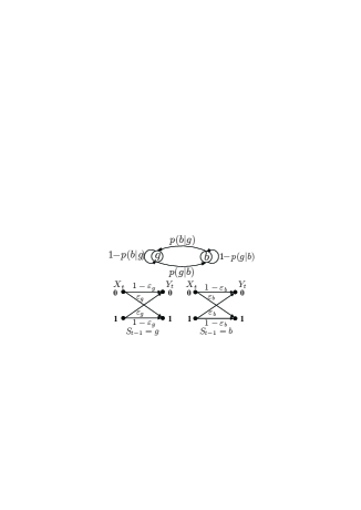
Figure 2: A Gilbert-Elliott channel.

III Channel Capacities and Upper bounds

III-A Channel Capacities

In order to unify the presentations of both channel capacities (the feedforward capacity and the feedback capacity), we use the notion of directed information, which was introduced by Massey in [4]. For any given joint probability distribution ${\rm Pr}\left(x^{N},y^{N}\right)$, the directed information from the channel input sequence $X^{N}$ to channel output sequence $Y^{N}$ is defined as

$$I\left(X^{N}\rightarrow Y^{N}\right)\stackrel{{\scriptstyle\Delta}}{{=}}\sum_{t=1}^{N}\,I\!\left(X^{t};Y_{t}\left|Y^{t-1}\right.\!\right).$$

It has been shown that $I\left(X^{N}\rightarrow Y^{N}\right)\leq I\left(X^{N};Y^{N}\right)$ with equality if the channel is used without feedback [4]. For simplicity, we denote $\mathcal{I}\left(X\rightarrow Y\right)$ as the directed information rate from the channel input to the channel output, that is,

$$\mathcal{I}\left(X\rightarrow Y\right)\stackrel{{\scriptstyle\Delta}}{{=}}\liminf_{N\rightarrow\infty}\frac{1}{N}\,I\!\left(X^{N}\rightarrow Y^{N}\right).$$ (4)

We now prove that the capacities can be characterized by the suprema of the directed information rates.

Theorem 1

The feedforward capacity of a stationary indecomposable noncontrollable FSC is given by

$$C=\sup_{\left\{{\rm Pr}\left(x_{t}\left|x^{t-1}\right.\!\right)\right\}_{t=1}^{\infty}}\mathcal{I}\left(X\rightarrow Y\right)$$ (5)

where the supremum is taken over all possible channel input processes. The feedback capacity of a stationary indecomposable noncontrollable FSC is given by

$$C^{fb}=\sup_{\left\{{\rm Pr}\left(x_{t}\left|x^{t-1},y^{t-1}\right.\!\right)\right\}_{t=1}^{\infty}}\mathcal{I}(X\rightarrow Y)$$ (6)

where the supremum is taken over all possible channel input processes that are causally dependent on the past channel outputs. This means that all past channel outputs $Y^{t-1}$ must be fed back to the source before emitting the symbol $X_{t}$.

Proof:

See Appendix A. ∎

For the general FSC, based on certain sufficient statistics, a dynamic programming framework to evaluate the capacity was presented [8]. However, as mentioned in Section VIII of [8], the sufficient statistic for a general FSC is often too complicated to be employed in dynamic programming methods. For some special FSCs, efficient dynamic programming algorithms have been proposed to evaluate the feedback capacity numerically [16, 28, 32, 33]. The main objective of this paper is to develop numerically computable upper bounds on the capacities of general indecomposable noncontrollable FSCs (2) with/without feedback.

III-B Upper Bounds on Capacities

To upper-bound the capacities, a technique of inserting the delayed channel state into the channel input is employed. Then the directed information from the channel input and delayed channel state sequence to the channel output sequence can be well defined as follows.

Definition 1

For a stationary indecomposable noncontrollable FSC (2), the directed information rate $\mathcal{I}_{v}\!\left(X,S\rightarrow Y\right)$ is defined as

$$\mathcal{I}_{v}\left(X,S\rightarrow Y\right)\stackrel{{\scriptstyle\Delta}}{{=}}\liminf_{N\rightarrow\infty}\frac{1}{N}\sum_{t=1}^{N}I\!\left(X^{t},S_{0}^{t-v-1};Y_{t}\left|Y^{t-1}\right.\!\right).$$ (7)

❑

In this definition, the $v$-delayed channel state is considered as a part of the channel input. Obviously, for a given channel input process, there is a nested sequence of upper bounds on $\mathcal{I}\left(X\rightarrow Y\right)$ as

$$\mathcal{I}\left(X\rightarrow Y\right)\leq\cdots\leq\mathcal{I}_{v+1}\left(X,S\rightarrow Y\right)$$ (8)

$$\;\;\;\;\;\;\;\;\;\>\;\leq\mathcal{I}_{v}\left(X,S\rightarrow Y\right)\leq\cdots\leq\mathcal{I}_{0}\left(X,S\rightarrow Y\right)\!.$$

Furthermore, the capacities in Theorem 1 can be bounded as

$$\begin{array}[]{ccc}C&\leq&\sup\limits_{\left\{\text{Pr}\left(x_{t}|x^{t-1}\right)\right\}_{t=1}^{\infty}}\mathcal{I}_{v}\left(X,S\rightarrow Y\right)\\ C^{fb}&\leq&\sup\limits_{\left\{\text{Pr}\left(x_{t}|x^{t-1},y^{t-1}\right)\right\}_{t=1}^{\infty}}\mathcal{I}_{v}\left(X,S\rightarrow Y\right).\end{array}$$ (9)

These upper bounds, however, can not be easily evaluated because the source sets are too general to be specified with a few parameters. To develop simpler expressions for upper bounds, we need to define the following sources in a similar way to those in [29].

Definition 2

Assume that the u-delayed output feedback (FB) $Y^{t-u-1}$, and the v-delayed state information (SI) $S_{0}^{t-v-1}$ are available at the source just before the emission of $X_{t}$ (see Fig. 3). Then the channel input $X_{t}$ could be selected according to a preset conditional probability law ${\rm Pr}\!\left(x_{t}\!\left|x^{t-1},s_{0}^{t-v-1},y^{t-u-1}\right.\!\right)$. All such input processes $\left\{X_{t}\right\}$ are described by a set $\mathcal{P}(u,v)$, i.e.,

$$\mathcal{P}(u,v)\stackrel{{\scriptstyle\Delta}}{{=}}\left\{{\rm Pr}\!\left(x_{t}\!\left|x^{t-1},s_{0}^{t-v-1},y^{t-u-1}\right.\!\right)\right\}_{t=1}^{\infty}.$$

In other words, $\mathcal{P}(u,v)$ represents the set of all sources (channel inputs) with $u$-delayed FB and $v$-delayed SI. ❑

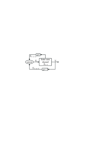
Figure 3: A noncontrollable FSC model with $u$-delayed FB and $v$-delayed SI.

Note that the delays $u$ and $v$ are both non-negative. An important subclass of sources from $\mathcal{P}(u,v)$, called conditional Markov source, is defined as follows.

Definition 3

For $v\leq m$, a source sequence $\{X_{t}\}$ used with $u$-delayed FB and $v$-delayed SI is said to be an m-th order conditional Markov source if the conditional probability mass function satisfies

$${\rm Pr}\!\left(x_{t}\!\left|x^{t-1}\!,s_{0}^{t-v-1}\!,y^{t-u-1}\right.\!\right)\!=\!{\rm Pr}\!\left(x_{t}\!\left|x_{t-m}^{t-1},s_{t-m-1}^{t-v-1},y^{t-u-1}\right.\!\right)\!.$$

Let $\mathcal{P}_{m}(u,v)$ represent the set of all such sources, that is,

$$\mathcal{P}_{m}(u,v)\stackrel{{\scriptstyle\Delta}}{{=}}\left\{{\rm Pr}\!\left(x_{t}\left|x_{t-m}^{t-1},s_{t-m-1}^{t-v-1},y^{t-u-1}\right.\!\right)\right\}_{t=1}^{\infty}.$$

❑

From the definitions of sources $\mathcal{P}(u,v)$ and $\mathcal{P}_{m}(u,v)$, we have the following facts for non-negative $u$, $v$ and $m$.

• The sets of channel input processes $\left\{{\rm Pr}\left(x_{t}\left|x^{t-1}\right.\right)\right\}_{t=1}^{\infty}$ and $\left\{{\rm Pr}\left(x_{t}\left|x^{t-1},y^{t-1}\right.\right)\right\}_{t=1}^{\infty}$ are subsets of the conditional source sets $\mathcal{P}(u,v)$ and $\mathcal{P}(0,v)$, respectively.

• $\mathcal{P}(u+1,v+1)\subseteq\mathcal{P}(u+1,v)\subseteq\mathcal{P}(u,v)$ and
  $\mathcal{P}(u+1,v+1)\subseteq\mathcal{P}(u,v+1)\subseteq\mathcal{P}(u,v)$.

• If $v+1\leq m$, then
  $\mathcal{P}_{m}(u+1,v+1)\subseteq\mathcal{P}_{m}(u+1,v)\subseteq\mathcal{P}_{m}(u,v)$ and
  $\mathcal{P}_{m}(u+1,v+1)\subseteq\mathcal{P}_{m}(u,v+1)\subseteq\mathcal{P}_{m}(u,v)$.

• If $v\leq m$, then $\mathcal{P}_{m}(u,v)\!\subseteq\!\mathcal{P}_{m+1}(u,v)\!\subseteq\!\cdots\!\subseteq\!\mathcal{P}(u,v)$.

Moreover, we can prove the following proposition.

Proposition 1

For a noncontrollable FSC with sources in the set $\mathcal{P}(u,u)$,

$${\rm Pr}\!\left(y_{t},s_{t}\!\left|x^{t+u},\!s_{0}^{t-1},y^{t-1}\right.\!\right)\!=\!{\rm Pr}\!\left(y_{t}\!\left|x_{t},\!s_{t-1}\right.\!\right){\rm Pr}\!\left(s_{t}\!\left|s_{t-1}\right.\!\right).$$ (10)

Proof:

In the case of $u=0$, equality (10) holds from the characteristics of the noncontrollable FSC in (2). In the case of $u\geq 1$, we have

$${\rm Pr}\!\left(y_{t},s_{t}\!\left|x^{t+u},s_{0}^{t-1},y^{t-1}\right.\!\right)$$ (11)

$$= \frac{{\rm Pr}\!\left(x^{t+u},s_{0}^{t},y^{t}\right)}{{\rm Pr}\!\left(x^{t+u},s_{0}^{t-1},y^{t-1}\right)}$$

$$= \frac{{\rm Pr}\!\left(x^{t},s_{0}^{t},y^{t}\right){\rm Pr}\!\left(x_{t+1}^{t+u}\!\left|x^{t},s_{0}^{t},y^{t}\right.\!\right)}{{\rm Pr}\!\left(x^{t},s_{0}^{t-1},y^{t-1}\right){\rm Pr}\!\left(x_{t+1}^{t+u}\!\left|x^{t},s_{0}^{t-1},y^{t-1}\right.\!\right)}$$

$$\stackrel{{\scriptstyle\rm(a)}}{{=}} {\rm Pr}\!\left(y_{t},s_{t}\!\left|x^{t},s_{0}^{t-1},y^{t-1}\right.\!\right)$$

$$= {\rm Pr}\!\left(y_{t}\!\left|x_{t},s_{t-1}\right.\!\right){\rm Pr}\!\left(s_{t}\left|s_{t-1}\right.\!\right)$$

where equality (a) results from the equality

$${\rm Pr}\!\left(x_{t+1}^{t+u}\!\left|x^{t},s_{0}^{t},y^{t}\right.\!\right)={\rm Pr}\!\left(x_{t+1}^{t+u}\!\left|x^{t},s_{0}^{t-1},y^{t-1}\right.\!\right)$$

since channel input processes are in the set $\mathcal{P}(u,u)=\left\{{\rm Pr}(x_{t}|x^{t-1},s_{0}^{t-u-1},y^{t-u-1})\right\}_{t=1}^{\infty}$ (see Definition 2). ∎

Proposition 1 implies that the probabilities ${\rm Pr}\left(y_{t},s_{t}\left|x^{t+u},s_{0}^{t-1},y^{t-1}\right.\right)$ are unaffected by the source selection from $\mathcal{P}(u,u)$ and that the probabilities ${\rm Pr}\left(y_{t},s_{t}\left|x^{t+u},s_{0}^{t-1},y^{t-1}\right.\right)$ can be characterized by the channel only. From the definition of the set $\mathcal{P}(u,u)$, we directly introduce a supremum as follows, which will be shown to be an upper bound on the capacity of the noncontrollable FSC.

Definition 4

Define $\mathcal{I}^{*}_{FB,SI}(u,v)$ as the supremum of the information rates $\mathcal{I}_{v}\left(X,S\rightarrow Y\right)$ over all sources with $u$-delayed FB and $u$-delayed SI in $\mathcal{P}(u,u)$, that is,

$$\mathcal{I}^{*}_{FB,SI}(u,v)\stackrel{{\scriptstyle\Delta}}{{=}}\sup\limits_{\mathcal{P}(u,u)}\mathcal{I}_{v}\left(X,S\rightarrow Y\right).$$ (12)

❑

Combining the inequalities in (8) and (9) with the discussion after Definitions 2 and 3, we conclude this section with the following proposition.

Proposition 2

1. For any $u\geq 0$ and $v\geq 0$, we have

   $$\mathcal{I}^{*}_{FB,SI}\left(u+1,v+1\right) \leq \mathcal{I}^{*}_{FB,SI}\left(u+1,v\right)$$

   $$\leq \mathcal{I}^{*}_{FB,SI}\left(u,v\right)$$

   and

   $$\mathcal{I}^{*}_{FB,SI}\left(u+1,v+1\right) \leq \mathcal{I}^{*}_{FB,SI}\left(u,v+1\right)$$

   $$\leq \mathcal{I}^{*}_{FB,SI}\left(u,v\right).$$

2. For any $v\geq 1$, we have a nested sequence of upper bounds on the feedforward capacity

   $$\begin{array}[]{ccl}C\leq\cdots\!\!\!\!&\leq&\!\!\!\!\mathcal{I}^{*}_{FB,SI}\left(v,v\right)\leq\cdots\\ \!\!\!\!&\leq&\!\!\!\!\mathcal{I}^{*}_{FB,SI}\left(1,1\right)\leq\mathcal{I}^{*}_{FB,SI}\left(0,0\right).\end{array}$$

3. For any $v\geq 1$, we have a nested sequence of upper bounds on the feedback capacity

   $$\begin{array}[]{ccl}C^{fb}\leq\cdots\!\!\!\!&\leq&\!\!\!\!\mathcal{I}^{*}_{FB,SI}\left(0,v\right)\leq\cdots\\ \!\!\!\!&\leq&\!\!\!\!\mathcal{I}^{*}_{FB,SI}\left(0,1\right)\leq\mathcal{I}^{*}_{FB,SI}\left(0,0\right).\end{array}$$

Proof:

It is straightforward and omitted here. ∎

IV Three Theorems for Upper Bounds

In this section, we introduce three main theorems that simplify the expressions for the upper bounds presented in Proposition 2 on the capacities of noncontrollable FSCs.

Theorem 2

Let $v\geq 0$. For noncontrollable FSCs,

$$I(X^{t},S_{0}^{t-v-1};Y_{t}|Y^{t-1})=I(X_{t-v}^{t},S_{t-v-1};Y_{t}|Y^{t-1})$$ (13)

and the directed information rate $\mathcal{I}_{v}\left(X,S\rightarrow Y\right)$ in (7) can be simplified as

$$\mathcal{I}_{v}\left(X,S\rightarrow Y\right)=\liminf\limits_{N\rightarrow\infty}\frac{1}{N}\sum\limits_{t=1}^{N}I(X_{t-v}^{t},S_{t-v-1};Y_{t}|Y^{t-1}).$$ (14)

Proof:

For any $v\geq 0$, by using the chain rule for mutual information, we have

$$I(X^{t},S_{0}^{t-v-1};Y_{t}|Y^{t-1})$$ (15)

$$= \!\!\!I(X_{t-v}^{t},S_{t-v-1};Y_{t}|Y^{t-1})$$

$$\!\!\!+\>I(X^{t-v-1},S_{0}^{t-v-2};Y_{t}|Y^{t-1},X_{t-v}^{t},S_{t-v-1}).$$

The last term equals zero since the current channel output $Y_{t}$ is independent of the distantly past states $S_{0}^{t-v-2}$ and inputs $X^{t-v-1}$ if the recent state $S_{t-v-1}$ and inputs $X_{t-v}^{t}$ and the whole history of outputs $Y^{t-1}$ are given. ∎

Theorem 3

Let $0\leq u\leq v$. The supremum $\mathcal{I}^{*}_{FB,SI}(u,v)$ is achieved by a $v$-th order conditional Markov source with $u$-delayed FB and $u$-delayed SI, that is,

$$\mathcal{I}^{*}_{FB,SI}(u,v)=\sup\limits_{\mathcal{P}_{v}(u,u)}\mathcal{I}_{v}(X,S\rightarrow Y)$$

where $\mathcal{P}_{v}(u,u)=\left\{{\rm Pr}\!\left(x_{t}\left|x_{t-v}^{t-1},s_{t-v-1}^{t-u-1},y^{t-u-1}\right.\!\right)\right\}_{t=1}^{\infty}$.

Proof:

See Appendix B. ∎

By Theorem 3, to evaluate the supremum $\mathcal{I}^{*}_{FB,SI}(u,v)$, it is necessary to search the whole set of conditional probabilities $\left\{{\rm Pr}\!\left(x_{t}\left|x_{t-v}^{t-1},s_{t-v-1}^{t-u-1},y^{t-u-1}\right.\!\right),t=1,2,\ldots,\right\}$. As time $t$ increases, the space of sequences $y^{t-u-1}$ expands exponentially, which makes it complicated to keep track of the dependence of the process $X_{t}$ on $Y^{t-u-1}$. In the sequel, we find some finite-size sufficient statistics to represent the sequence $y^{t-u-1}$.

Let $\mathcal{M}$ be the Cartesian product $\mathcal{X}^{v}\times\mathcal{S}^{v-u+1}$ whose elements are indexed simply by $\ell\in\{0,1,\cdots,M-1\}$ with $M=|\mathcal{M}|$. A random vector $\underline{A}_{t}$ is specified as the a posteriori probability vector with realization

$$\underline{\alpha}_{t}\stackrel{{\scriptstyle\Delta}}{{=}}\left[\alpha_{t}(0),\alpha_{t}(1),\cdots,\alpha_{t}(M-1)\right]$$ (16)

where

$$\alpha_{t}(\ell)\!\stackrel{{\scriptstyle\Delta}}{{=}}\!{\rm Pr}\!\left(\left(\!X_{t-v+1}^{t},\!S_{t-v}^{t-u}\!\right)\!=\!\ell\,|y^{t-u}\!\right)$$ (17)

for $\ell\!\in\!\{0,1,\cdots,M\!-\!1\}$. The sample space of the random vector $\underline{A}_{t}$ is denoted by $\mathcal{A}$, which is a simplex in $\mathbb{R}^{M}$. That is, $\mathcal{A}=\{\underline{\alpha}=\left[\alpha(0),\ldots,\alpha(M-1)\right]:\alpha(i)\geq 0,\sum_{i=0}^{M-1}\alpha(i)=1\}$. Given the probability vector $\underline{\alpha}_{t-1}$, the channel output $y_{t-u}$ and the set of transition probabilities ${\rm Pr}\!\left(x_{t}\!\left|x_{t-v}^{t-1},s_{t-v-1}^{t-u-1},y^{t-u-1}\right.\!\right)$, we can use the forward recursion of the BCJR algorithm [37] to compute all values of $\alpha_{t}(\ell)$ as

$$\alpha_{t}\!\left(x_{t-v+1}^{t},\!s_{t-v}^{t-u}\right)\!=\!\frac{\sum\limits_{x_{t-v},s_{t-v-1}}\!\!\!\!{\rm Pr}\!\left(x_{t-v}^{t},\!s_{t-v-1}^{t-u},\!y_{t-u}\!\left|y^{t-u-1}\right.\!\right)}{\sum\limits_{x_{t-v}^{t},s_{t-v-1}^{t-u}}\!\!\!\!{\rm Pr}\!\left(x_{t-v}^{t},\!s_{t-v-1}^{t-u},\!y_{t-u}\!\left|y^{t-u-1}\right.\!\right)}$$ (18)

where

$${\rm Pr}\!\left(\!x_{t\!-v}^{t},\!s_{t\!-v-\!1}^{t\!-u},\!y_{t\!-u}\!\left|y^{t\!-u-\!1}\right.\!\!\right)$$ (19)

$$\!\stackrel{{\scriptstyle\textrm{(a)}}}{{=}} \!\alpha_{t\!-1}\!\!\left(x_{t\!-v}^{t\!-1},s_{t\!-v-\!1}^{t\!-u-\!1}\right){\rm Pr}\!\left(x_{t}\!\left|x_{t\!-v}^{t\!-1},\!s_{t\!-v-\!1}^{t\!-u-\!1},\!y^{t\!-u-\!1}\right.\!\right)$$

$$\!\times\,{\rm Pr}\!\left(y_{t\!-u}\!\left|x_{t\!-u},s_{t\!-u-\!1}\right.\!\right)\!{\rm Pr}\!\left(s_{t\!-u}\!\left|s_{t\!-u-\!1}\right.\!\right).$$

The equality (a) results from Proposition 1 and the assumption $u\leq v$. From (19), we know that, once the prior conditional probability vector $\underline{\alpha}_{t-1}$ is given, the current conditional probability vector $\underline{\alpha}_{t}$ depends only on the current transition probability ${\rm Pr}\!\left(\!x_{t}\!\left|x_{t-v}^{t-1},\!s_{t-v-1}^{t-u-1},\!y^{t-u-1}\right.\!\right)$ and the channel transition law. To shorten the notation, we abbreviate (18) and (19) as

$$\underline{\alpha}_{t}\!=\!F_{\rm BCJR}\!\left(\underline{\alpha}_{t-\!1},\!\left\{{\rm Pr}\!\left(\!x_{t}\!\!\left|x_{t-\!v}^{t-\!1},\!s_{t-v-\!1}^{t-u-\!1},\!y^{t-u-\!1}\right.\!\right)\!\right\}\!,y_{t-u}\!\right)\!.$$ (20)

Evidently, the vector $\underline{\alpha}_{t-1}$ depends on the sequence $y^{t-u-1}$, and two different sequences $y^{t-u-1}$ and $\tilde{y}^{t-u-1}$ may result in the same vectors $\underline{\alpha}_{t-1}$. For an arbitrarily selected source from $\mathcal{P}_{v}(u,u)$, two different sequences $y^{t-u-1}$ and $\tilde{y}^{t-u-1}$ may induce different probabilities

$${\rm Pr}\!\left(x_{t}\!\left|x_{t-v}^{t-1},s_{t-v-1}^{t-u-1},y^{t-u-1}\right.\!\right)\!\neq\!{\rm Pr}\!\left(x_{t}\!\left|x_{t-v}^{t-1},s_{t-v-1}^{t-u-1},\tilde{y}^{t-u-1}\right.\!\right).$$

However, there do exist sources such that different sequences $y^{t-u-1}$ and $\tilde{y}^{t-u-1}$ resulting in the same vectors $\underline{\alpha}_{t-1}=\underline{\tilde{\alpha}}_{t-1}$ induce the same probabilities

$${\rm Pr}\!\left(x_{t}\!\left|x_{t-v}^{t-1},s_{t-v-1}^{t-u-1},y^{t-u-1}\right.\!\right)\!=\!{\rm Pr}\!\left(x_{t}\!\left|x_{t-v}^{t-1},s_{t-v-1}^{t-u-1},\tilde{y}^{t-u-1}\right.\!\right).$$

Such a subclass of $\mathcal{P}_{v}(u,u)$ is defined as follows.

Definition 5

The set $\mathcal{P}^{\prime}_{v}(u,u)$ collects all the $v$-th order conditional Markov sources with $u$-delayed FB and $u$-delayed SI such that

$${\rm Pr}\!\left(x_{t}\!\left|x_{t-v}^{t-1},s_{t-v-1}^{t-u-1},y^{t-u-1}\right.\!\right)\!=\!{\rm Pr}\!\left(x_{t}\!\left|x_{t-v}^{t-1},s_{t-v-1}^{t-u-1},\tilde{y}^{t-u-1}\right.\!\right)$$

whenever ${\underline{\alpha}}_{t-1}=\tilde{\underline{\alpha}}_{t-1}$. Hence, the source set $\mathcal{P}^{\prime}_{v}(u,u)$ can be shortly denoted by

$$\mathcal{P}^{\prime}_{v}(u,u)\stackrel{{\scriptstyle\Delta}}{{=}}\left\{{\rm Pr}\!\left(x_{t}\!\left|x_{t-v}^{t-1},s_{t-v-1}^{t-u-1},\underline{\alpha}_{t-1}\right.\!\right)\right\}_{t=1}^{\infty}.$$

❑

Fig. 4 depicts the noncontrollable FSC model, whose source belongs to the set $\mathcal{P}^{\prime}_{v}(u,u)$.

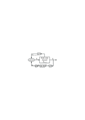
Figure 4: A noncontrollable FSC whose source is in the set $\mathcal{P}^{\prime}_{v}(u,u)$.

Theorem 4

Let $u\!\leq\!v$. The supremum $\mathcal{I}^{*}_{FB,SI}\!\left(u,\!v\right)$ can be achieved by a source in the set $\mathcal{P}^{\prime}_{v}(u,\!u)$, that is,

$$\mathcal{I}^{*}_{FB,SI}(u,v)=\sup_{\mathcal{P}^{\prime}_{v}(u,u)}\mathcal{I}_{v}\left(X,S\rightarrow Y\right)$$ (21)

where $\mathcal{P}^{\prime}_{v}(u,u)=\left\{{\rm Pr}\!\left(x_{t}\!\left|x_{t-v}^{t-1},s_{t-v-1}^{t-u-1},\underline{\alpha}_{t-1}\right.\!\right)\right\}_{t=1}^{\infty}$.

Proof:

See Appendix C. ∎

V DYNAMIC PROGRAMMING FOR SOURCE OPTIMIZATION

V-A Stochastic Control Formulations

From Theorem 4, we only need to consider the sources in the set $\mathcal{P}^{\prime}_{v}(u,u)$. In this setting, for any given $y^{t-u-1}$,

$${\rm Pr}\!\left(x_{t-v}^{t},s_{t-v-1},y_{t-u}^{t}\!\left|y^{t-u-1}\right.\right)$$ (22)

$$= \sum_{s_{t-v}^{t-u}}{\rm Pr}\!\left(x_{t-v}^{t},s_{t-v-1}^{t-u},y_{t-u}^{t}\!\left|y^{t-u-1}\right.\right)$$

$$\stackrel{{\scriptstyle\rm(a)}}{{=}} \sum_{s_{t-v}^{t-u}}{\rm Pr}\!\left(\!x_{t\!-\!v}^{t\!-\!1},\!s_{t\!-\!v\!-\!1}^{t\!-\!u\!-\!1}\left|y^{t\!-\!u\!-\!1}\right.\!\right){\rm Pr}\!\left(\!x_{t}\!\left|x_{t\!-\!v}^{t\!-\!1},\!s_{t\!-\!v\!-\!1}^{t\!-\!u\!-\!1},\!y^{t\!-\!u\!-\!1}\right.\!\right)$$

$$\>\>\>\>\>\>\>\times\;{\rm Pr}\!\left(y_{t\!-\!u}\left|x_{t\!-\!u},\!s_{t\!-\!u\!-\!1}\right.\!\right){\rm Pr}\left(s_{t\!-\!u}\!\left|s_{t\!-\!u\!-\!1}\right.\!\right)$$

$$\>\>\>\>\>\>\>\times\;{\rm Pr}\!\left(y_{t\!-\!u+1}^{t}\!\left|x_{t\!-\!v}^{t},\!s_{t\!-\!v\!-\!1}^{t\!-\!u}\right.\!\right)$$

$$\stackrel{{\scriptstyle\rm(b)}}{{=}} \sum_{s_{t-v}^{t-u}}\alpha_{t\!-\!1}\!\!\left(\!x_{t\!-\!v}^{t\!-\!1},\!s_{t\!-\!v\!-\!1}^{t\!-\!u\!-\!1}\!\right){\rm Pr}\!\left(\!x_{t}\!\left|x_{t\!-\!v}^{t\!-\!1},\!s_{t\!-\!v\!-\!1}^{t\!-\!u\!-\!1},\!\underline{\alpha}_{t-1}\right.\!\right)$$

$$\>\>\>\>\>\>\>\times\;{\rm Pr}\!\left(y_{t\!-\!u}\left|x_{t\!-\!u},\!s_{t\!-\!u\!-\!1}\right.\!\right){\rm Pr}\left(s_{t\!-\!u}\!\left|s_{t\!-\!u\!-\!1}\right.\!\right)$$

$$\>\>\>\>\>\>\>\times\;{\rm Pr}\!\left(y_{t\!-\!u+1}^{t}\!\left|x_{t\!-\!v}^{t},\!s_{t\!-\!v\!-\!1}^{t\!-\!u}\right.\!\right)$$

where equality (a) results from Proposition 1 and the assumption $u\leq v$, and equality (b) results directly from the definition of the source set $\mathcal{P}^{\prime}_{v}(u,u)$. Similar to equation (60) as shown in Appendix B, we can prove that the conditional probability ${\rm Pr}\!\left(y_{t-u+1}^{t}\left|x_{t-v}^{t},s_{t-v-1}^{t-u}\right.\!\right)$ is completely determined by the channel law. Therefore, equalities in (22) indicate that the joint conditional probability mass function on the left-hand side of (22) is not sensitive to the vector $y^{t-u-1}$ (that appears in the conditioning clause) but to its induced variable $\underline{\alpha}_{t-1}$. This implies that

$$I\!\left(X_{t-v}^{t},S_{t-v-1};Y_{t}\!\left|Y_{t-u+1}^{t-1},y_{t-u},y^{t-u-1}\right.\right)$$ (23)

$$=I\!\left(X_{t-v}^{t},S_{t-v-1};Y_{t}\!\left|Y_{t-u+1}^{t-1},y_{t-u},\underline{\alpha}_{t-1}\right.\right)$$

of which the right-hand side is a function of $\underline{\alpha}_{t-1}$, $\left\{{\rm Pr}\!\left(x_{t}\!\left|x_{t-v}^{t-1},s_{t-v-1}^{t-u-1},\underline{\alpha}_{t-1}\right.\!\right)\right\}$ and $y_{t-u}$. For simplicity, we introduce the following notations

$$\begin{array}[]{ccc}{\rm p}_{t}(\underline{\alpha}_{t-1})&\stackrel{{\scriptstyle\Delta}}{{=}}&\left\{{\rm Pr}\!\left(x_{t}\!\left|x_{t-v}^{t-1},s_{t-v-1}^{t-u-1},\underline{\alpha}_{t-1}\right.\!\right)\right\}\\ {\rm p}_{t}&\stackrel{{\scriptstyle\Delta}}{{=}}&\left\{{\rm p}_{t}(\underline{\alpha}_{t-1}):\underline{\alpha}_{t-1}\in\mathcal{A}\right\}\end{array}.$$

Obviously, for $\underline{\alpha}_{t-1}\in\mathcal{A}$, the quantity ${\rm p}_{t}(\underline{\alpha}_{t-1})$ is a transition probability matrix of size $M\times|\mathcal{X}|$. Let $\mathscr{P}$ be the collection of all possible transition probability matrices. Both of the sets $\mathcal{A}$ and $\mathscr{P}$ are bounded and closed, and hence compact. Moreover, $\left\{\{{\rm p}_{t}\}_{t=1}^{\infty}\right\}=\{({\rm p}_{1},{\rm p}_{2},\cdots)\}=\mathcal{P}^{\prime}_{v}(u,u)$. Then the right-hand side of (23) is a function that can be denoted by

$$g\left(\underline{\alpha}_{t-1},{\rm p}_{t}(\underline{\alpha}_{t-1}),y_{t-u}\right)$$ (24)

$$\stackrel{{\scriptstyle\Delta}}{{=}}I\!\left(X_{t-v}^{t},S_{t-v-1};Y_{t}\!\left|Y_{t-u+1}^{t-1},y_{t-u},\underline{\alpha}_{t-1}\right.\right).$$

Therefore, we can rewrite the directed information rate $\mathcal{I}_{v}(X,S\rightarrow Y)$ in (14) as

$$\mathcal{I}_{v}\!\left(X,S\rightarrow Y\right)$$ (25)

$$= \!\!\!\liminf_{N\!\rightarrow\!\infty}\!\frac{1}{N}\sum_{t=1}^{N}I\!\left(X_{t-v}^{t},S_{t-v-1};Y_{t}\!\left|Y_{t-u+1}^{t-1},Y^{t-u}\right.\!\right)$$

$$= \!\!\!\liminf_{N\!\rightarrow\!\infty}\!\frac{1}{N}\mathbf{E}\!\left[\sum_{t=1}^{N}g\left(\underline{\alpha}_{t-1},{\rm p}_{t}(\underline{\alpha}_{t-1}),Y_{t-u}\right)\!\right]\!.$$

Substituting (25) into (21), we can see that the problem to find the upper bound $\mathcal{I}^{*}_{FB,SI}(u,v)$ is equivalent to the following discrete-time infinite-horizon average reward per stage stochastic control problem (ARSCP) [35, 36, 38], which is referred to as Problem A for convenience.

Problem A. The ARSCP is specified as follows.

1. The stochastic control system of the problem is characterized by

   $$\underline{\alpha}_{t}\!=\!F_{BCJR}\!\left(\underline{\alpha}_{t-1},{\rm p}_{t}(\underline{\alpha}_{t-1}),y_{t-u}\right)$$ (26)

   where

   1. $\underline{\alpha}_{t-1}$ is the state and $\mathcal{A}$ is the state space, i.e., $\underline{\alpha}_{t-1}\in\mathcal{A}$ and $\underline{\alpha}_{t}\in\mathcal{A}$;

   2. ${\rm p}_{t}$ is the function (or policy) that maps the state space $\mathcal{A}$ to the action space $\mathscr{P}$, and ${\rm p}_{t}(\underline{\alpha}_{t-1})\in\mathscr{P}$ is the policy (or control) when the state is $\underline{\alpha}_{t-1}$;

   3. $y_{t-u}$ is the disturbance.

2. The reward function at stage $t$ is $g\!\left(\underline{\alpha}_{t-1},{\rm p}_{t}(\underline{\alpha}_{t-1}),y_{t-u}\right)$. For convenience, we define the expected reward function at stage $t$ as

   $$g\left(\underline{\alpha}_{t-1},{\rm p}_{t}(\underline{\alpha}_{t-1})\right)$$ (27)

   $$= {\bf E}\left[g\left(\underline{\alpha}_{t-1},{\rm p}_{t}(\underline{\alpha}_{t-1}),Y_{t-u}\right)\right]$$

   $$= I\left(X_{t-v}^{t},S_{t-v-1};Y_{t}\left|Y_{t-u}^{t-1},\underline{\alpha}_{t-1}\right.\right).$$

3. The objective of this problem is to find the maximum average reward per stage, i.e.,

   $$\mathcal{I}(\underline{\alpha}_{0}\!)=\!\!\sup\limits_{\{{\rm p}_{t}\}\in\mathcal{P}^{\prime}_{v}(u,u)}\!\!\!\!\!\!\mathcal{I}(\underline{\alpha}_{0},\{{\rm p}_{t}\})~{}{\rm for~{}all}~{}\underline{\alpha}_{0}\!\!\in\!\mathcal{A}$$ (28)

   where $\mathcal{I}(\underline{\alpha}_{0},\{{\rm p}_{t}\})$ is the average reward associated with the initial state $\underline{\alpha}_{0}$ and the sequence of policies $\{{\rm p}_{t}\}$

   $$\mathcal{I}\!\left(\underline{\alpha}_{0},\{{\rm p}_{t}\}\!\right)\!=\!\liminf_{N\rightarrow\infty}\!\frac{1}{N}\mathbf{E}\!\left[\sum\limits_{t=1}^{N}g\!\left(\underline{\alpha}_{t-1},{\rm p}_{t}(\underline{\alpha}_{t-1}),Y_{t-u}\right)\!\right]\!\!.$$ (29)

For the stochastic dynamic system (26) of Problem A, we have following two propositions.

Proposition 3

The system disturbance variable $Y_{t-u}$ is characterized by a conditional probability distribution that depends explicitly on the system state $\underline{\alpha}_{t-1}$ and the policy $\left\{{\rm Pr}\!\left(x_{t}\!\left|x_{t-v}^{t-1},s_{t-v-1}^{t-u-1},\underline{\alpha}_{t-1}\right.\!\right)\right\}$ (i.e., ${\rm p}_{t}(\underline{\alpha}_{t-1})$).

Proof:

Given the system state $\underline{\alpha}_{t-1}$ and the policy $\left\{{\rm Pr}\!\left(x_{t}\!\left|x_{t-v}^{t-1},s_{t-v-1}^{t-u-1},\underline{\alpha}_{t-1}\right.\!\right)\right\}$, the probability mass function of the system disturbance can be explicitly determined as

$${\rm Pr}\!\left(y_{t\!-\!u}\!\left|\underline{\alpha}_{t\!-\!1},\!\left\{\!{\rm Pr}\!\left(x_{t}\!\left|x_{t\!-\!v}^{t\!-\!1},s_{t\!-\!v\!-\!1}^{t\!-\!u\!-\!1},\underline{\alpha}_{t\!-\!1}\right.\!\right)\!\right\}\right.\!\right)$$ (30)

$$= \!\!\!\!\!\!\!\!\sum_{x_{t\!-\!v}^{t},s_{t\!-\!v\!-\!1}^{t\!-\!u}}\!\!\!\!\!{\rm Pr}\!\left(x_{t\!-\!v}^{t},s_{t\!-\!v\!-\!1}^{t\!-\!u},y_{t\!-\!u}\!\left|\underline{\alpha}_{t\!-\!1},\!\left\{\!{\rm Pr}\!\left(x_{t}\!\left|x_{t\!-\!v}^{t\!-\!1},s_{t\!-\!v-\!1}^{t\!-\!u\!-\!1},\underline{\alpha}_{t\!-\!1}\right.\!\right)\!\right\}\right.\!\right)$$

$$\stackrel{{\scriptstyle\textrm{(a)}}}{{=}} \!\!\!\!\!\!\!\!\sum_{x_{t\!-\!v}^{t},s_{t\!-\!v\!-\!1}^{t\!-\!u}}\!\!\!\!\!\alpha_{t\!-\!1}\!\!\left(\!x_{t\!-\!v}^{t\!-\!1},\!s_{t\!-\!v\!-\!1}^{t\!-\!u\!-\!1}\!\right){\rm Pr}\!\left(\!x_{t}\!\left|x_{t\!-\!v}^{t\!-\!1},\!s_{t\!-\!v\!-\!1}^{t\!-\!u\!-\!1},\!\underline{\alpha}_{t\!-\!1}\right.\!\right)$$

$$\;\;\;\;\;\times\;{\rm Pr}\!\left(y_{t\!-\!u}\left|x_{t\!-\!u},\!s_{t\!-\!u\!-\!\!1}\right.\!\right){\rm Pr}\!\left(s_{t\!-\!u}\!\left|s_{t\!-\!u\!-\!\!1}\right.\!\right)$$

where equality (a) follows from Proposition 1 and the assumption $u\!\leq\!v$. ∎

Proposition 4

The state process $\underline{A}_{t}$ with realization $\underline{\alpha}_{t}$ is a Markov process.

Proof:

Equation (26) and Proposition 3 imply that, given the prior state $\underline{A}_{t-1}$, the current state $\underline{A}_{t}$ is independent of the early states $\underline{A}_{0}^{t-2}$. Hence, $\underline{A}_{t}$ is a Markov process. ∎

Proposition 5

The reward function $g\!\left(\underline{\alpha}_{t\!-\!1},{\rm p}_{t}(\underline{\alpha}_{t\!-\!1}\!),y_{t\!-\!u}\!\right)$ is uniformly continuous over $\mathcal{A}\times\mathscr{P}$.

Proof:

This proposition can be proved by the compactness of the set $\mathcal{A}\times\mathscr{P}$ and the continuity of the reward function. ∎

In the average reward problem, i.e., Problem A, both the state $\underline{\alpha}$ and the policy ${\rm p}_{t}(\underline{\alpha})$ are continuous, which causes difficulties in theoretical analysis as well as computation. Fortunately, the uniform continuity of the reward function make it reasonable to restrict the reward function on discretized (finite) state space and action space. This approach causes a loss at most $\varepsilon$ as long as the quantization is fine enough [35, Sec. 6.6]. That is, Problem A can be solved approximately (resulting in an $\varepsilon$-optimal value) by solving its discretized version, Problem B.

Problem B. Let $\mathcal{Q}_{\delta}(\cdot)$ be a quantizer of the state set $\mathcal{A}$ which results in a finite-state space $\hat{\mathcal{A}}\subset\mathcal{A}$. Specifically, for any state $\underline{\alpha}\in\mathcal{A}$, there exists a quantized state $\hat{\underline{\alpha}}\in\hat{\mathcal{A}}$ such that the Euclidean distance satisfies $\|\underline{\alpha}-\hat{\underline{\alpha}}\|\leq\delta$ where $\delta$ is the designated quantization parameter. Similarly, let $\mathcal{Q}_{\xi}(\cdot)$ be the quantizer of the action space $\mathscr{P}$ and the resulting finite set be denoted by $\hat{\mathscr{P}}$. The finite-state and finite-action ARSCP is specified as follows.

1. The stochastic control system of this problem is

   $$\hat{\underline{\alpha}}_{t}=\mathcal{Q}_{\delta}\left(F_{BCJR}(\hat{\underline{\alpha}}_{t-1},\hat{\rm p}_{t}(\hat{\underline{\alpha}}_{t-1}),y_{t-u})\right)$$ (31)

   where

   1. $\hat{\underline{\alpha}}_{t-1}$ is the state and $\hat{\mathcal{A}}$ is the state space;

   2. $\hat{{\rm p}}_{t}$ is the function (or policy) that maps the state space $\hat{\mathcal{A}}$ to the action space $\hat{\mathscr{P}}$, and $\hat{{\rm p}}_{t}(\hat{\underline{\alpha}}_{t-1})\in\hat{\mathscr{P}}$ is the policy when the state is $\hat{\underline{\alpha}}_{t-1}$;

   3. $y_{t-u}$ is the disturbance.

2. The reward function at stage $t$ is $g\!\left(\hat{\underline{\alpha}}_{t-1},\hat{\rm p}_{t}(\hat{\underline{\alpha}}_{t-1}),y_{t-u}\right)$.

3. The objective of this problem is to find the maximum average reward per stage, i.e.,

   $$\mathcal{I}(\hat{\underline{\alpha}}_{0})\!=\!\!\sup_{\hat{\mathcal{P}}^{\prime}_{v}(u,u)}\!\!\mathcal{I}\!\left(\hat{\underline{\alpha}}_{0},\{\hat{\rm p}_{t}\}\right)~{}{\rm for~{}all}~{}\hat{\underline{\alpha}}_{0}\in\hat{\mathcal{A}}$$ (32)

   where

   • $\hat{\mathcal{P}}^{\prime}_{v}(u,u)$ is the collection of all policy sequences $\{\hat{\rm p}_{t}\}_{t=1}^{\infty}$ and is regarded as a discretized version of the source set $\mathcal{P}^{\prime}_{v}(u,u)$;

   • $\mathcal{I}(\hat{\underline{\alpha}}_{0},\{\hat{\rm p}_{t}\})$ is the average reward associated with the initial state $\hat{\underline{\alpha}}_{0}$ and the sequence of policies $\{\hat{\rm p}_{t}\}$

     $$\!\!\!\!\!\!\!\mathcal{I}\!\left(\hat{\underline{\alpha}}_{0},\!\{\hat{\rm p}_{t}\}\!\right)\!=\!\liminf_{N\rightarrow\infty}\!\frac{1}{N}\mathbf{E}\!\left[\sum\limits_{t=1}^{N}g\!\left(\hat{\underline{\alpha}}_{t-1},\hat{\rm p}_{t}(\hat{\underline{\alpha}}_{t-1}\!),\!Y_{t-u}\right)\!\right]\!\!.$$ (33)

The pair of coupled optimality equations [35, 40] of Problem B are

$$G^{*}(\underline{\alpha})=\max_{{\rm p}(\underline{\alpha})\in\hat{\mathscr{P}}}{\bf E}_{\underline{A}^{\prime}|\underline{\alpha}}\left[G^{*}(\underline{A}^{\prime})\right],~{}{\rm for~{}any}~{}\underline{\alpha}\in\hat{\mathcal{A}}$$ (34)

and

$$\!\!\!\!\!\!\!\!G^{*}\!(\underline{\alpha})+J^{*}\!(\underline{\alpha})$$ (35)

$$\!\!\!\!\!\!\!\!\!\!\!\!\!\!\!\!\!\!\!\!\!\!= \!\!\!\!\!\!\!\!\!\!\!\!\!\!\!\!\max\limits_{{\rm p}(\underline{\alpha})\in\bar{\mathscr{P}}(\underline{\alpha})}\!\!\!\left\{g\!\left(\underline{\alpha},{\rm p}(\underline{\alpha})\!\right)\!+\!\mathbf{E}_{\underline{A}^{\prime}|\underline{\alpha}}\!\!\left[J^{*}\!(\underline{A}^{\prime})\!\right]\!\right\},\!~{}{\rm for~{}any}~{}\underline{\alpha}\!\in\!\hat{\mathcal{A}}$$

where $\bar{\mathscr{P}}(\underline{\alpha})=\left\{{\rm p}(\underline{\alpha}):{\rm p}(\underline{\alpha})\in\arg\max_{\hat{\mathscr{P}}}{\bf E}_{\underline{A}^{\prime}|\underline{\alpha}}\left[{G}^{*}(\underline{A}^{\prime})\right]\right\}$ is the set of policies attaining the maximum in equation (34). The pair of coupled optimality equations can also be represented by vectors as

$$G^{*}=\max_{{\rm p}\in\mathcal{D}}L_{{\rm p}}G^{*}$$ (36)

and

$$G^{*}+J^{*}=\max_{{\rm p}\in\bar{\mathcal{D}}}\left\{g+L_{{\rm p}}J^{*}\right\}$$ (37)

where $\mathcal{D}$ is the set of all possible policies, i.e., $\mathcal{D}=\left\{{\rm p}=\left\{{\rm p}(\underline{\alpha}):\underline{\alpha}\in\hat{\mathcal{A}}\right\}\right\}$, and $\bar{\mathcal{D}}$ is the set of policies attaining the maximum in (36), i.e., $\bar{\mathcal{D}}=\left\{{\rm p}\in\mathcal{D}:{\rm p}\in\arg\max L_{{\rm p}}G^{*}\right\}$, and $L_{{\rm p}}=\left[{\rm Pr}(\underline{\alpha}^{\prime}|\underline{\alpha},{\rm p}(\underline{\alpha}))\right]_{|\hat{\mathcal{A}}|\times|\hat{\mathcal{A}}|}$ is a transition matrix between states under the policy ${\rm p}$. The solution $(G^{*},J^{*})$ to the pair of coupled optimality equations is usually called the gain-bias pair [36, 40] with $G^{*}$ being the optimal average reward vector. The policy that achieves the maxima in the pair of coupled optimality equations is called the optimal policy.

Remark: Depending on the choice of stationary policy, the Markov chain $\{\underline{A}_{t}\in\hat{\mathcal{A}}\}$ of Problem B may have different recurrent classes. Hence, Problem B is in general a multi-chain model [36]. The pair of coupled optimality equations of Problem B can be viewed as an analog to the Bellman equation for the uni-chain model [35, 36].

Theorem 5

For Problem B, there exists a stationary policy that satisfies the pair of coupled optimality equations (34) and (35).

Proof:

See Appendix D. ∎

From Theorem 5, it suffices to investigate only stationary policies. For convenience, we denote

$${\rm Pr}(j|i,\underline{\alpha})\!\stackrel{{\scriptstyle\Delta}}{{=}}\!{\rm Pr}\!\left(X_{t}=j\!\left|\left(X_{t-v}^{t-1},S_{t-v-1}^{t-u-1}\!\right)=i,\underline{A}_{t-1}=\underline{\alpha}\right.\!\right).$$

Then the stationary policy in the discretized version of the source set $\mathcal{P}^{\prime}_{v}(u,u)$ can be denoted by

$${\rm p}=\left\{{\rm p}(\underline{\alpha})=\left\{{\rm Pr}(j|i,\underline{\alpha})\right\}:\underline{\alpha}\in\hat{\mathcal{A}}\right\}.$$

We note that with a stationary source ${\rm p}$, the directed information rate $\mathcal{I}_{v}(X,S\rightarrow Y)$ in (25) can be computed using Monte Carlo methods similar to those in [21, 22, 23, 24].

V-B A Value Iteration Method to Solve Problem B

For a finite-state and finite-action ARSCP, there exist several dynamic programming algorithms (such as value iteration, policy iteration and linear programming) [36] to solve the pair of coupled optimality equations. To obtain $\varepsilon$-optimal value with small $\varepsilon$, fine quantization is required, but then the discretized state space $\hat{\mathcal{A}}$ and action space $\hat{\mathscr{P}}$ usually have large sizes. In this setting, the value iteration method is a better choice. In this subsection, a value iteration algorithm is introduced to solve Problem B. Under a mild assumption, the presented value iteration algorithm is shown to be convergent and delivers the near-optimal stationary policy and the optimal average reward value numerically.

The value iteration method is, for all $\underline{\alpha}\in\hat{\mathcal{A}}$,

$$J_{k}(\underline{\alpha})=\max_{\hat{\mathscr{P}}}\left\{g(\underline{\alpha},{\rm p}(\underline{\alpha}))+{\bf E}_{\underline{A}^{\prime}|\underline{\alpha}}\left[J_{k-1}(\underline{A}^{\prime})\right]\right\}$$ (38)

starting from an arbitrary initial function $J_{0}$. In the following, we show that this value iteration method can deliver a solution $(G^{*},J^{*})$ to the pair of coupled optimality equations (34) and (35). On one hand, from Proposition 4.3.1 in [36], the optimal average reward vector $G^{*}$ can be obtained as

$$G^{*}=\lim_{k\rightarrow\infty}\frac{J_{k}}{k}.$$ (39)

Note that in general, for a multi-chain average reward problem, $G^{*}(\underline{\alpha})$ may be different for different $\underline{\alpha}$. But by performing the iteration method for Example 1, we find that the values $\frac{J_{k}(\underline{\alpha})}{k}$ are always numerically approaching a constant as $k\rightarrow\infty$.

On the other hand, we need to find $J^{*}$. To this end, we make an additional assumption as follows.

Assumption 1

Every optimal stationary policy $\rm p$ has an aperiodic transition probability matrix $L_{\rm p}$. ❑

Remark: Recall that

$$\underline{\alpha}_{t}=\left[\alpha_{t}(0),\alpha_{t}(1),\cdots,\alpha_{t}(M-1)\right]$$ (40)

and

$$\alpha_{t}(\ell)={\rm Pr}\!\left(\left(\!X_{t-v+1}^{t},\!S_{t-v}^{t-u}\!\right)\!=\!\ell\,|y^{t-u}\!\right).$$ (41)

Intuitively, the optimal stationary policy should not depend heavily on the early channel outputs. In other words, the influence of $y^{t-w-1}$ on the optimal policy should die away with sufficiently large $w$. Specifically, for two different channel output sequences $(y^{t-w-1},y_{t-w}^{t-u})$ and $(\tilde{y}^{t-w-1},y_{t-w}^{t-u})$, the resulting probability vectors $\underline{\alpha}_{t}$ and ${\tilde{\underline{\alpha}}_{t}}$ should be almost the same (i.e., their Euclidean distance should be very small). As a result, the quantized versions of $\underline{\alpha}_{t}$ and ${\underline{\tilde{\alpha}}}_{t}$ will be equal. This implies that, for a given optimal stationary policy, the states $\underline{A}_{t}\in\mathcal{A}$ can be restricted to the subset of states (called it the subset of effective states) that correspond to the most recent channel outputs $Y_{t-w}^{t-u}$. Such a subset is communicative. In particular, the state $\underline{\alpha}$ corresponding to the vector $Y_{t-w}^{t-u}=\underline{0}$ can be reached from itself whenever the next channel output $Y_{t-u+1}$ equals $0$. Hence, the Markov chain is essentially aperiodic. This intuition has also been verified numerically in our example.

Under Assumption 1, according to Propositions 4.3.5 and 4.3.6 in [36], we have the following facts.

1. The optimal average reward vector $G^{*}$ satisfying (39) can also be obtained by

   $$G^{*}=\lim_{k\rightarrow\infty}(J_{k}-J_{k-1}).$$ (42)

2. The bias $J^{*}$ can be obtained by

   $$J^{*}=\lim_{k\rightarrow\infty}(J_{k}-kG^{*}).$$ (43)

3. There exists a sufficiently large $K$ such that for any $k\geq K$,

   $$\!\!\!\!\!\!\!\!\max_{{\rm p}(\underline{\alpha})\in\hat{\mathscr{P}}}\!\left\{g(\underline{\alpha},{\rm p}(\underline{\alpha}))+{\bf E}_{\underline{A}^{\prime}|\underline{\alpha}}\left[J_{k-1}(\underline{A}^{\prime})\right]\right\}$$ (44)

   $$\!\!\!\!= \!\!\!\!\!\!\!\!\max\limits_{{\rm p}(\underline{\alpha})\in\bar{\mathscr{P}}(\underline{\alpha})}\!\left\{g(\underline{\alpha},{\rm p}(\underline{\alpha}))+{\bf E}_{\underline{A}^{\prime}|\underline{\alpha}}\left[J_{k-1}(\underline{A}^{\prime})\right]\right\}$$

   where $\bar{\mathscr{P}}(\underline{\alpha})$ has been defined in the previous subsection, see equation (35).

Therefore, the pair $(G^{*},J^{*})$ induced by the value iteration method (38) is a solution to the pair of coupled optimality equations (34) and (35). Moreover, let ${\rm p}$ be the policy obtained by the value iteration method (38) for the sufficiently large $K$. Then $\{{\rm p}\}^{\infty}$ can achieve numerically optimal average reward value of Problem B. A practical value iteration algorithm for Problem B is described as follows.

Algorithm 1 (A Value Iteration Algorithm)

1. Initialization:

   • Choose a large positive integer $n$.

   • Initialize the terminal reward function or starting vector as $J_{0}(\underline{\alpha})=0$ for all $\underline{\alpha}\in\hat{\mathcal{A}}$.

2. Recursions:
   For $k\!=\!1,2,\ldots,n$, and any $\underline{\alpha}\in\hat{\mathcal{A}}$, compute

   $$J_{k}(\underline{\alpha})\!=\!\!\!\max_{{\rm p}(\underline{\alpha})\in\hat{\mathscr{P}}}\!\!\left\{g\!\left(\underline{\alpha},\!{\rm p}(\underline{\alpha})\right)\!+\!\mathbf{E}_{\underline{A}^{\prime}|\underline{\alpha}}\left[J_{k-1}(\underline{A}^{\prime})\right]\!\right\}\!.$$ (45)

   where $\underline{A}^{\prime}\in\hat{\mathcal{A}}$ is the random variable that depends on the system disturbance variable $Y_{t-u}$, and where the realization $\underline{\alpha}^{\prime}$ of $\underline{A}^{\prime}$ can be computed by

   $$\underline{\alpha}^{\prime}\!=\mathcal{Q}_{\delta}\!\left(F_{BCJR}\!\left(\underline{\alpha},{\rm p}(\underline{\alpha}),y_{t-u}\right)\right).$$ (46)

3. Optimized source:
   For any $\underline{\alpha}\in\hat{\mathcal{A}}$, the optimized source distribution is delivered as

   $${\rm p}^{*}(\underline{\alpha})=\arg\!\max_{{\rm p}(\underline{\alpha})\in\hat{\mathscr{P}}}\!\left\{\!g\!\left(\underline{\alpha},\!{\rm p}(\underline{\alpha})\right)\!+\!\!\mathbf{E}_{\underline{A}^{\prime}|\underline{\alpha}}\left[J_{n}(\underline{A}^{\prime})\right]\!\right\}.$$ (47)

4. End.

Remark: By implementing Algorithm 1, we can obtain stationary Markov source probabilities ${\rm p}^{*}=\left\{{\rm p}^{*}(\underline{\alpha}):\underline{\alpha}\in\hat{\mathcal{A}}\right\}$, which can be utilized to evaluate numerically the optimal average reward of Problem B, i.e., the $\varepsilon$-optimal value of Problem A. Strictly speaking, the optimal stationary policy ${\rm p}^{*}$ obtained in (47) for Problem B is an approximation of the optimal stationary policy of Problem A, and the information rate $\mathcal{I}_{v}\left(X,S\rightarrow Y\right)$ induced by the “optimal” stationary policy ${\rm p}^{*}$ is only a lower bound on the upper bound $\mathcal{I}_{FB,SI}^{*}(u,v)$. Obviously, finer quantization of $\mathcal{A}$ and $\mathscr{P}$ should cause less loss of optimality. The numerical values resulting from different quantizations are discussed in the following section.

VI Numerical results

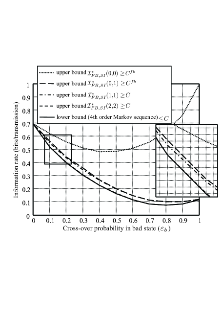
Figure 5: Bounds on the capacities of the RLL$(1,\infty)$-GE channel.

In this section, we present numerical results by taking the RLL$(1,\infty)$-GE channel shown in Fig. 1 and Fig. 2 as an example. We chose this channel because it was already used in a prior publication [26]. In this example, we set the transition probabilities between the channel states as $p(b\!\left|g\right.)\!=\!p(g\!\left|b\right.)\!=\!0.3$, the cross-over probability in the “good” state as $\varepsilon_{g}\!=\!0.001$ and the cross-over probability in the “bad” state as a variable $\varepsilon_{b}\in[0,1]$. Firstly, we quantize the state space $\mathcal{A}$ and the action space $\mathscr{P}$ using parameters $\delta$ and $\xi$, respectively. Secondly, we apply Algorithm 1 introduced in Section V to obtain an “optimal” stationary policy. Finally, we use Monte Carlo methods [21, 22, 23, 24] to numerically evaluate the upper bounds $\mathcal{I}^{*}_{FB,SI}(u,v)$. The results are shown in Fig. 5, where $\mathcal{I}^{*}_{FB,SI}(1,1)$ and $\mathcal{I}^{*}_{FB,SI}(2,2)$ are two upper bounds on the feedforward capacity, and $\mathcal{I}^{*}_{FB,SI}(0,0)$ and $\mathcal{I}^{*}_{FB,SI}(0,1)$ are two upper bounds on the feedback capacity. As expected, $\mathcal{I}^{*}_{FB,SI}(2,2)\leq\mathcal{I}^{*}_{FB,SI}(1,1)\leq\mathcal{I}^{*}_{FB,SI}(0,1)\leq\mathcal{I}^{*}_{FB,SI}(0,0)$. It is worth pointing out that, due to the RLL constraints, the source must have memory of order at least one and the optimization is implemented by taking into account the RLL constraint. In particular, the upper bound $\mathcal{I}^{*}_{FB,SI}(0,0)$ is obtained by optimizing the sources $\mathcal{P}^{\prime}_{1}(0,0)$. Also shown in Fig. 5 is a lower bound on $C$ computed using techniques presented in [25, 26]. By comparing $\mathcal{I}^{*}_{FB,SI}(2,2)$ with the lower bound, we observe that the bounds $\mathcal{I}^{*}_{FB,SI}(v,v)$ are numerically tight upper bounds on the feedforward capacity. We are unable to evaluate the tightness of the upper bounds $\mathcal{I}^{*}_{FB,SI}(0,v)$ on the feedback capacity since no good lower bounds on $C^{fb}$ are available in the literature for noncontrollable FSCs.

Fig. 6 illustrates the loss of the optimality caused by quantization. We focus on the computation of $\mathcal{I}^{*}_{FB,SI}(1,1)$. Let the quantization parameter of the action space $\mathscr{P}$ be fixed, i.e., $\xi=0.0125$, and the quantization parameter $\delta$ of the state space $\mathcal{A}$ be varying. From Fig. 6, we can see that a smaller $\delta$ (equivalently, a finer quantizer) induces a larger information rate $\mathcal{I}_{1}(X,S\rightarrow Y)$ and causes less loss of optimality. It can also be seen that the gap between the different quantizers is negligible for small quantization parameters $\delta$.

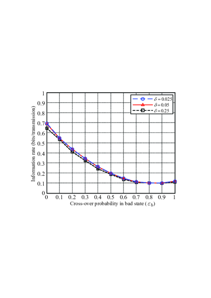
Figure 6: Information rates $\mathcal{I}_{1}(X,S\rightarrow Y)$ for “optimal” quantized sources in $\mathcal{P}^{\prime}_{1}(1,1)$ delivered by Algorithm 1 with different quantizers, where the quantization parameters of the state space and the action space are $\delta$ and $\xi=0.0125$, respectively.

VII Conclusion

By the technique of inserting the delayed channel state into the channel input, the directed information rate from the new channel input (including the channel input and the delayed channel state) to the channel output is defined, and then a universal form of upper bounds on the capacities of the noncontrollable FSC has been developed. In particular, two respective nested sequences of upper bounds on the feedforward capacity and the feedback capacity are obtained. It has been shown that these upper bounds can be achieved by finite order conditional Markov sources with delayed output feedback (FB) and delayed state information (SI). Moreover, the computation of the upper bounds was formulated as an average reward per stage stochastic control problem (ARSCP) with a continuous state space and a continuous action space. By the compactness of the state space and the action space and the unform continuity of the reward function, the original ARSCP was transformed into an ARSCP with a finite state set and a finite action set, which can be solved by a value iteration algorithm. Under a mild assumption, the value iteration algorithm is shown to be convergent and delivers a near-optimal stationary policy as well as numerically tight upper bounds.

Appendix A Proof of Theorem 1

Proof:

The feedforward capacity in (5) and the feedback capacity in (6) are rewritten as

$$C=\sup_{\left\{{\rm Pr}\left(x_{t}\left|x^{t-1}\right.\!\right)\right\}_{t=1}^{\infty}}\liminf_{N\rightarrow\infty}\frac{1}{N}I(X^{N}\rightarrow Y^{N})$$ (48)

and

$$C^{fb}=\sup_{\left\{{\rm Pr}\left(x_{t}\left|x^{t-1},y^{t-1}\right.\!\right)\right\}_{t=1}^{\infty}}\liminf_{N\rightarrow\infty}\frac{1}{N}I(X^{N}\rightarrow Y^{N}),$$ (49)

respectively. We now prove that they are equal to the capacities

$$C_{G}=\lim_{N\rightarrow\infty}\sup_{\left\{{\rm Pr}(x_{t}|x^{t-1})\right\}_{t=1}^{N}}\frac{1}{N}I(X^{N}\rightarrow Y^{N})$$ (50)

defined by Gallager in [11, Theorems 4.6.4 and 5.9.1] and

$$C_{P}^{fb}=\lim_{N\rightarrow\infty}\sup_{\left\{{\rm Pr}(x_{t}|x^{t-1},y^{t-1})\right\}_{t=1}^{N}}\frac{1}{N}I(X^{N}\rightarrow Y^{N})$$ (51)

defined by Permuter et al. in [13, Theorem 18], respectively. Here, we only prove $C=C_{G}$. A similar method (omitted here) can be used to prove $C^{fb}=C_{P}^{fb}$.

On one hand, we have $C\leq C_{G}$. Let $\left\{{\rm Pr}^{*}\!\left(x_{t}\left|x^{t-1}\right.\!\right)\right\}_{t=1}^{\infty}$ be a sequence of sources that achieves the capacity $C$. Then, for each $N$ and the fixed sequence $\left\{{\rm Pr}^{*}\!\left(x_{t}\left|x^{t-1}\right.\!\right)\right\}_{t=1}^{N}$, the corresponding directed information $I^{*}(X^{N}\rightarrow Y^{N})$ is less than $\sup I(X^{N}\rightarrow Y^{N})$, which implies that $C\leq C_{G}$.

On the other hand, we prove $C_{G}\leq C$. To this end, we introduce a new capacity expression

$$C_{M}=\sup_{\left\{\left\{{\rm Pr}(x_{t}|x^{t-1})\right\}_{t=1}^{T}\right\}_{T=1}^{\infty}}\liminf_{N\rightarrow\infty}\frac{1}{N}I(X^{N}\rightarrow Y^{N})\vspace{-0.1cm}$$ (52)

where the supremum is taken over all possible sequences of sources without the consistency requirement, i.e., $\left\{\left\{{\rm Pr}(x_{t}|x^{t-1})\right\}_{t=1}^{T}\right\}_{T=1}^{\infty}$. Firstly, we prove that $C_{G}\leq C_{M}$. For each $N$, denote the optimal source achieving $\sup I(X^{N}\rightarrow Y^{N})$ as $\left\{{\rm Pr}^{*}(x_{t}|x^{t-1})\right\}_{t=1}^{N}$. For the fixed sequence of sources $\left\{\left\{{\rm Pr}^{*}(x_{t}|x^{t-1})\right\}_{t=1}^{T}\right\}_{T=1}^{\infty}$, $\liminf\frac{1}{N}I(X^{N}\rightarrow Y^{N})=C_{G}$ trivially holds. Thus we have $C_{G}\leq C_{M}$. Secondly, we prove that $C_{M}=C$. It is obvious that $C\leq C_{M}$ since $\left\{{\rm Pr}(x_{t}|x^{t-1})\right\}_{t=1}^{\infty}\subset\left\{\left\{{\rm Pr}(x_{t}|x^{t-1})\right\}_{t=1}^{T}\right\}_{T=1}^{\infty}$. Now we need to prove that $C<C_{M}$ does not hold. Otherwise, there must exist a sequence of sources $\left\{\left\{{\rm{\tilde{P}r}}(x_{t}|x^{t-1})\right\}_{t=1}^{T}\right\}_{T=1}^{\infty}$ such that $\liminf_{N\rightarrow\infty}\frac{1}{N}I(X^{N}\rightarrow Y^{N})\geq C+\epsilon_{0}$ where $\epsilon_{0}>0$. It implies that there exists a $K$ such that for all $N\geq K$, $\frac{1}{N}I(X^{N}\rightarrow Y^{N})\geq C+\epsilon$ where $0<\epsilon<\epsilon_{0}$. Let $\left\{{\rm{\tilde{P}r}}(x_{t}|x^{t-1})\right\}_{t=1}^{N}$ be the source for a fixed $N\geq K$. Construct a process by $X^{\infty}=X^{N}\times X^{N}\times\cdots$ with probability assignment ${\rm Pr}(x^{\infty})=\left({\rm Pr}(x^{N})\right)^{\infty}$. Consider the directed information rate $\frac{1}{NL}I(X^{NL}\rightarrow Y^{NL})$.

$$\frac{1}{NL}I(X^{NL}\rightarrow Y^{NL})$$

$$\!\!\!\!\!= \!\!\!\!\!\!\frac{1}{NL}\sum_{i=1}^{NL}I(X^{i};Y_{i}|Y^{i-1})$$

$$\!\!\!\!\!= \!\!\!\!\!\!\frac{1}{NL}\sum_{\ell=0}^{L-1}\sum_{i=1}^{N}I(X^{\ell N+i};Y_{\ell N+i}|Y^{\ell N+i-1})$$

$$\!\!\!\!\!\geq \!\!\!\!\!\!\frac{1}{NL}\sum_{\ell=0}^{L-1}\sum_{i=1}^{N}I(X_{\ell N+1}^{\ell N+i};Y_{\ell N+i}|Y^{\ell N+i-1})$$

$$\!\!\!\!\!= \!\!\!\!\!\!\frac{1}{NL}\sum_{\ell=0}^{L-1}\sum_{i=1}^{N}I(X_{\ell N+1}^{\ell N+i};Y_{\ell N+i}|Y_{\ell N+1}^{\ell N+i-1},Y^{\ell N})$$

$$\!\!\!\!\!\stackrel{{\scriptstyle\rm(a)}}{{\geq}} \!\!\!\!\!\!\frac{1}{NL}\sum_{\ell=0}^{L-1}\left(\!\!\!\begin{array}[]{l}-\log|\mathcal{S}|\\ +\sum\limits_{i=1}^{N}I(X_{\ell N+1}^{\ell N+i};Y_{\ell N+i}|Y_{\ell N+1}^{\ell N+i-1},Y^{\ell N},S_{\ell N})\end{array}\!\!\!\!\!\right)$$

$$\!\!\!\!\!\stackrel{{\scriptstyle\rm(b)}}{{=}} \!\!\!\!\!\!\frac{1}{NL}\sum_{\ell=0}^{L-1}\left(\!\!-\log|\mathcal{S}|+\sum_{i=1}^{N}I(X_{\ell N+1}^{\ell N+i};Y_{\ell N+i}|Y_{\ell N+1}^{\ell N+i-1}\!,\!S_{\ell N})\!\!\right)$$

$$\!\!\!\!\!\stackrel{{\scriptstyle\rm(c)}}{{\geq}} \!\!\!\!\!\!\frac{1}{NL}\sum_{\ell=0}^{L-1}\left(\!\!-2\log|\mathcal{S}|+\sum_{i=1}^{N}I(X_{\ell N+1}^{\ell N+i};Y_{\ell N+i}|Y_{\ell N+1}^{\ell N+i-1})\!\!\right)$$

$$\!\!\!\!\!= \!\!\!\!\!\!\frac{1}{NL}\sum_{\ell=0}^{L-1}\left(-2\log|\mathcal{S}|+I(X_{\ell N+1}^{\ell N+N}\rightarrow Y_{\ell N+1}^{\ell N+N})\right)$$

$$\!\!\!\!\!\stackrel{{\scriptstyle\rm(d)}}{{=}} \!\!\!\!\!\!\frac{1}{N}\left(-2\log|\mathcal{S}|+I(X^{N}\rightarrow Y^{N})\right)$$

$$\!\!\!\!\!\geq \!\!\!\!\!\!C+\epsilon-\frac{2}{N}\log|\mathcal{S}|$$ (56)

where inequalities (a) and (c) result from Lemma 4 in [13], equality (b) results from the Markovianity of the chain $(X^{\ell N},Y^{\ell N})\rightarrow S_{\ell N}\rightarrow(X_{\ell N+1}^{(\ell+1)N},Y_{\ell N+1}^{(\ell+1)N})$, and equality (d) results from the assumptions of channel model and the construction of the process which imply that $I(X_{\ell N+1}^{\ell N+N}\rightarrow Y_{\ell N+1}^{\ell N+N})=I(X^{N}\rightarrow Y^{N})$ for all $\ell$. By the choice of $\epsilon_{0}$ and $\epsilon$, for any $L$, $\frac{1}{NL}I(X^{NL}\rightarrow Y^{NL})>C+\delta$ where $\delta>0$. Then $\liminf\frac{1}{N}I(X^{N}\rightarrow Y^{N})>C$, which raises a contradiction, regarding the expression of $C$ in (48). Therefore, $C_{G}\leq C_{M}=C$. ∎

Appendix B Proof of Theorem 3

Proof:

Let $\mathcal{P}_{1}\!\in\!\mathcal{P}(u,u)$ be an arbitrary source with $u$-delayed FB and $u$-delayed SI. Denote the corresponding information as $I\left(\left.X_{t-v}^{t},S_{t-v-1};Y_{t}\right|Y^{t-1}\right)$. To prove Theorem 3, it is sufficient to show that there exists a conditional Markov source $\mathcal{P}_{2}$ in $\mathcal{P}_{v}(u,u)\subseteq\mathcal{P}(u,u)$ with the same information $I\left(\left.X_{t-v}^{t},S_{t-v-1};Y_{t}\right|Y^{t-1}\right)$ as that achieved by $\mathcal{P}_{1}$. To do this, for any given $\mathcal{P}_{1}\!\in\!\mathcal{P}(u,u)$, we construct a new source $\mathcal{P}_{2}\in\mathcal{P}_{v}(u,u)$ as

$${\rm Pr}^{\left(\mathcal{P}_{2}\right)}\left(x_{t}\left|x^{t-1},s_{0}^{t-u-1},y^{t-u-1}\right.\right)$$ (57)

$$\stackrel{{\scriptstyle\Delta}}{{=}}{\rm Pr}^{\left(\mathcal{P}_{1}\right)}\left(x_{t}\left|x_{t-v}^{t-1},s_{t-v-1}^{t-u-1},y^{t-u-1}\right.\right)$$

with the initial probability as

$${\rm Pr}^{(\mathcal{P}_{2})}\!\left(x^{v},s_{0}^{v-u},y^{v-u}\!\right)\!\stackrel{{\scriptstyle\Delta}}{{=}}\!{\rm Pr}^{(\mathcal{P}_{1})}\!\left(x^{v},s_{0}^{v-u},y^{v-u}\!\right).$$

In the following, we will prove that both $\mathcal{P}_{1}$ and $\mathcal{P}_{2}$ induce the same joint probability distribution ${\rm Pr}\!\left(x_{t-v}^{t},\!s_{t-v-1},\!y^{t}\right)$, which, together with the result of Theorem 2, completes the proof of Theorem 3.

Actually, for any source with $u$-delayed FB and $u$-delayed SI, we have

$${\rm Pr}\!\left(x_{t-v}^{t},\!s_{t-v-1},\!y^{t}\right)$$ (58)

$$\!\!\!\!\!\!= \!\!\!\!\!\!\!\!\!\sum_{x^{t\!-\!v\!-\!1},s_{0}^{t\!-\!v\!-\!2},s_{t\!-\!v}^{t\!-\!u}}\!\!\!\!\!\!\!\!\!\!{\rm Pr}\!\left(x^{t},s_{0}^{t-u},y^{t}\right)$$

$$\!\!\!\!\!\!= \!\!\!\!\!\!\!\!\!\sum_{x^{t\!-\!v\!-\!1},s_{0}^{t\!-\!v\!-\!2},s_{t\!-\!v}^{t\!-\!u}}\!\!\!\!\!\!\!\!\!\!{\rm Pr}\!\left(x^{t},s_{0}^{t-u},y^{t-u}\right){\rm Pr}\!\left(\left.y_{t-u+1}^{t}\right|x^{t},s_{0}^{t-u},y^{t-u}\right)$$

$$\!\!\!\!\!\!= \!\!\!\!\!\!\!\!\!\sum_{x^{t\!-\!v\!-\!1},s_{0}^{t\!-\!v\!-\!2},s_{t\!-\!v}^{t\!-\!u}}\!\!\!\!\!\!\!\!\!\!{\rm Pr}\!\left(x^{v},s_{0}^{v-u},y^{v-u}\right){\rm Pr}\!\left(\left.y_{t-u+1}^{t}\right|x^{t},s_{0}^{t-u},y^{t-u}\right)$$

$$\;\;\;\;\;\;\times\prod_{\tau=v+1}^{t}\!\!{\rm Pr}\!\left(x_{\tau}\left|x^{\tau-1},s_{0}^{\tau-u-1},y^{\tau-u-1}\!\right.\right)$$

$$\;\;\;\;\;\;\;\;\;\;\;\;\;\;\;\;\times\,{\rm Pr}\!\left(y_{\tau-u},s_{\tau-u}\left|x^{\tau},s_{0}^{\tau-u-1},y^{\tau-u-1}\!\right.\right)$$

The channel laws ${\rm Pr}\!\left(y_{\tau-u},s_{\tau-u}\!\left|x^{\tau},s_{0}^{\tau-u-1},y^{\tau-u-1}\right.\!\right)$ and ${\rm Pr}\left(\left.y_{t-u+1}^{t}\right|x^{t},s_{0}^{t-u},y^{t-u}\right)$ in the above equation are both independent of the source distribution $\mathcal{P}_{1}$ (or $\mathcal{P}_{2}$) since

$${\rm Pr}\left(y_{\tau-u},s_{\tau-u}\left|x^{\tau},s_{0}^{\tau-u-1},y^{\tau-u-1}\right.\right)$$ (59)

$$\stackrel{{\scriptstyle\rm(a)}}{{=}} \!\!\!{\rm Pr}\left(y_{\tau-u}\left|x_{\tau-u},s_{\tau-u-1}\right.\right){\rm Pr}\left(s_{\tau-u}\left|s_{\tau-u-1}\right.\right)$$

$$\stackrel{{\scriptstyle\rm(b)}}{{=}} \!\!\!{\rm Pr}\left(y_{\tau-u},s_{\tau-u}\left|x_{\tau-v}^{\tau},s_{\tau-v-1}^{\tau-u-1},y^{\tau-u-1}\right.\right)$$

and

$${\rm Pr}\left(\left.y_{t-u+1}^{t}\right|x^{t},s_{0}^{t-u},y^{t-u}\right)$$ (60)

$$= \sum_{s_{t-u+1}^{t}}{\rm Pr}\left(\left.y_{t-u+1}^{t},s_{t-u+1}^{t}\right|x^{t},s_{0}^{t-u},y^{t-u}\right)$$

$$= \sum_{s_{t-u+1}^{t}}\prod_{\tau=t-u+1}^{t}{\rm Pr}\left(\left.y_{\tau},s_{\tau}\right|x^{t},s_{0}^{\tau-1},y^{\tau-1}\right)$$

$$\stackrel{{\scriptstyle\rm(c)}}{{=}} \sum_{s_{t-u+1}^{t}}\prod_{\tau=t-u+1}^{t}{\rm Pr}\left(\left.y_{\tau}\right|x_{\tau},s_{\tau-1}\right){\rm Pr}\left(\left.s_{\tau}\right|s_{\tau-1}\right)$$

$$\stackrel{{\scriptstyle\rm(d)}}{{=}} \sum_{s_{t-u+1}^{t}}\prod_{\tau=t-u+1}^{t}{\rm Pr}\left(\left.y_{\tau},s_{\tau}\right|x_{t-v}^{t},s_{t-v-1}^{\tau-1},y^{\tau-1}\right)$$

$$= {\rm Pr}\left(\left.y_{t-u+1}^{t}\right|x_{t-v}^{t},s_{t-v-1}^{t-u},y^{t-u}\right)$$

where equalities (a), (b), (c) and (d) result from Proposition 1 and the assumption $u\leq v$. Equalities (a) and (c) also state that the conditional probabilities ${\rm Pr}\!\left(y_{\tau\!-\!u},s_{\tau\!-\!u}\left|x^{\tau}\!,\!s_{0}^{\tau\!-\!u\!-\!1},\!y^{\tau\!-\!u-1}\right.\!\right)$ and ${\rm Pr}\!\left(\!\left.y_{t-u+1}^{t}\right|x^{t}\!,\!s_{0}^{t\!-\!u},\!y^{t\!-\!u}\!\right)$ are completely determined by the channel transition law.

Therefore, using (59) and (60), the given source $\mathcal{P}_{1}\!\in\!\mathcal{P}(u,u)$ induces the joint probability

$${\rm Pr}^{(\mathcal{P}_{1})}\!\!\left(x_{t-v}^{t},s_{t-v-1},y^{t}\right)$$ (61)

$$\!\!\!\!\!\!= \!\!\!\!\!\!\!\!\!\!\!\sum_{x^{t\!-\!v\!-\!1}\!,s_{0}^{t\!-\!v\!-\!2}\!,s_{t\!-\!v}^{t\!-\!u}}\!\!\!\!\!\!\!\!\!\!\!\!\!{\rm Pr}^{(\mathcal{P}_{1})}\!\!\left(x^{v}\!,s_{0}^{v-u}\!,y^{v-u}\!\right){\rm Pr}\!\left(\left.\!y_{t-u+1}^{t}\!\right|\!x_{t-v}^{t},s_{t-v-1}^{t-u},y^{t-u}\!\right)$$

$$\;\;\;\;\times\!\prod_{\tau={v+1}}^{t}\!\!{\rm Pr}^{(\mathcal{P}_{1})}\!\!\left(x_{\tau}\left|x^{\tau-1},s_{0}^{\tau-u-1},y^{\tau-u-1}\!\right.\right)$$

$$\;\;\;\;\;\;\;\;\;\;\;\;\times\;{\rm Pr}\!\left(y_{\tau-u},s_{\tau-u}\!\left|x_{\tau-v}^{\tau},s_{\tau-v-1}^{\tau-u-1},y^{\tau-u-1}\right.\!\right)$$

and the conditional probability

$${\rm Pr}^{(\mathcal{P}_{1})}\!\left(x_{t}\left|x_{t-v}^{t-1},s_{t-v-1}^{t-u-1},y^{t-u-1}\right.\right)$$ (62)

$$= \frac{{\rm Pr}^{(\mathcal{P}_{1})}\!\left(x_{t-v}^{t},s_{t-v-1}^{t-u-1},y^{t-u-1}\right)}{{\rm Pr}^{(\mathcal{P}_{1})}\!\left(x_{t-v}^{t-1},s_{t-v-1}^{t-u-1},y^{t-u-1}\right)}$$

$$= \frac{\sum\limits_{x^{t-v-1},s_{0}^{t-v-2}}{\rm Pr}^{(\mathcal{P}_{1})}\!\left(x^{t},s_{0}^{t-u-1},y^{t-u-1}\right)}{\sum\limits_{x^{t-v-1},s_{0}^{t-v-2}}{\rm Pr}^{(\mathcal{P}_{1})}\!\left(x^{t-1},s_{0}^{t-u-1},y^{t-u-1}\right)}$$ (63)

where

$${\rm Pr}^{(\mathcal{P}_{1})}\!\!\left(x^{t}\!,s_{0}^{t\!-\!u\!-\!1}\!,y^{t\!-\!u\!-\!1}\right)$$

$$\!= \!\!{\rm Pr}^{(\mathcal{P}_{1})}\!\!\left(\!x^{t\!-\!1}\!,\!s_{0}^{t\!-\!u\!-\!1}\!,\!y^{t\!-\!u\!-\!1}\right){\rm Pr}^{(\mathcal{P}_{1})}\!\!\left(\!x_{t}\!\left|x^{t\!-\!1}\!,\!s_{0}^{t\!-\!u\!-\!1}\!,\!y^{t\!-\!u\!-\!1}\right.\!\right)\!$$

and

$${\rm Pr}^{(\mathcal{P}_{1})}\!\left(x^{t-1},s_{0}^{t-u-1},y^{t-u-1}\right)$$

$$= \!\!\!{\rm Pr}^{(\mathcal{P}_{1})}\!\left(x^{v},s_{0}^{v-u},y^{v-u}\right)$$

$$\!\!\times\!\prod\limits_{\tau=v+1}^{t-1}\!\!{\rm Pr}^{\left(\mathcal{P}_{1}\right)}\!\left(x_{\tau}\!\left|x^{\tau-1},s_{0}^{\tau-u-1},y^{\tau-u-1}\right.\!\right)$$

$$\>\>\>\>\>\>\>\>\times\,{\rm Pr}\!\left(y_{\tau-u}\!\left|x_{\tau-u},s_{\tau-u-1}\right.\!\right){\rm Pr}\!\left(s_{\tau-u}\!\left|s_{\tau-u-1}\right.\!\right).$$

On the other hand, the source $\mathcal{P}_{2}\in\!\mathcal{P}_{v}(u,u)$ constructed as (57) induces the joint probability shown in (64) (see the top of the following page),

$${\rm Pr}^{(\mathcal{P}_{2})}\!\left(x_{t-v}^{t},s_{t-v-1},y^{t}\right)$$ (64)

$$\!\!\!\!\!\!\!\!= \!\!\!\!\!\!\!\!\!\!\!\!\sum_{x^{t\!-\!v\!-\!1}\!,s_{0}^{t\!-\!v\!-\!2}\!,s_{t\!-\!v}^{t\!-\!u}}\!\!\!\!\!\!\!\!\!\!\!\!\!{\rm Pr}^{(\mathcal{P}_{2})}\!\!\left(x^{v}\!,s_{0}^{v\!-\!u}\!,y^{v\!-\!u}\right)\!{\rm Pr}\!\left(\!\left.y_{t\!-\!u\!+\!1}^{t}\!\right|\!x_{t\!-\!v}^{t},s_{t\!-\!v\!-\!1}^{t\!-\!u},y^{t\!-\!u}\right)\!\!\!\prod_{\tau={v\!+\!1}}^{t}\!\!\!{\rm Pr}^{(\mathcal{P}_{2})}\!\!\left(x_{\tau}\!\left|x^{\tau\!-\!1}\!,s_{0}^{\tau\!-\!u\!-\!1}\!,y^{\tau\!-\!u\!-\!1}\!\right.\right)\!{\rm Pr}\!\left(y_{\tau\!-\!u},s_{\tau\!-\!u}\!\left|x_{\tau\!-\!v}^{\tau},s_{\tau\!-\!v\!-\!1}^{\tau\!-\!u\!-\!1},y^{\tau\!-\!u\!-\!1}\!\right.\right)$$

$$\!\!\!\!\!\!\!\!\stackrel{{\scriptstyle\textrm{(e)}}}{{=}} \!\!\!\!\!\!\!\!\!\!\!\!\sum_{x^{t\!-\!v\!-\!1}\!,s_{0}^{t\!-\!v\!-\!2}\!,s_{t\!-\!v}^{t\!-\!u}}\!\!\!\!\!\!\!\!\!\!\!\!\!{\rm Pr}^{(\mathcal{P}_{1})}\!\!\left(x^{v}\!,s_{0}^{v\!-\!u}\!,y^{v\!-\!u}\right)\!{\rm Pr}\!\left(\!\left.y_{t\!-\!u\!+\!1}^{t}\!\right|\!x_{t\!-\!v}^{t},s_{t\!-\!v\!-\!1}^{t\!-\!u},y^{t\!-\!u}\right)\!\!\!\prod_{\tau=v\!+\!1}^{t}\!\!\!{\rm Pr}^{\left(\mathcal{P}_{1}\right)}\!\!\left(x_{\tau}\!\left|x_{\tau\!-\!v}^{\tau\!-\!1}\!,s_{\tau\!-\!v\!-\!1}^{\tau\!-\!u\!-\!1}\!,y^{\tau\!-\!u\!-\!1}\!\right.\right)\!{\rm Pr}\!\left(y_{\tau\!-\!u},s_{\tau\!-\!u}\!\left|x_{\tau\!-\!v}^{\tau},s_{\tau\!-\!v\!-\!1}^{\tau\!-\!u\!-\!1},y^{\tau\!-\!u\!-\!1}\!\right.\right)$$

$$\!\!\!\!\!\!\!\!\stackrel{{\scriptstyle\textrm{(f)}}}{{=}} \!\!\!\!\!\!\!\!\!\!\!\!\sum_{x^{t\!-\!v\!-\!1}\!,s_{0}^{t\!-\!v\!-\!2}\!,s_{t\!-\!v}^{t\!-\!u}}\!\!\!\!\!\!\!\!\!\!\!\!\!{\rm Pr}^{(\mathcal{P}_{1})}\!\!\left(x^{v}\!,s_{0}^{v\!-\!u}\!,y^{v\!-\!u}\right)\!{\rm Pr}\!\left(\left.y_{t\!-\!u\!+\!1}^{t}\!\right|\!x_{t\!-\!v}^{t},s_{t\!-\!v\!-\!1}^{t\!-\!u},y^{t\!-\!u}\right)\!\!\!\prod_{\tau=v\!+\!1}^{t}\!\frac{{\rm Pr}^{(\mathcal{P}_{1})}\!\left(x_{\tau-v}^{\tau},s_{\tau-v-1}^{\tau-u},y^{\tau-u}\right)}{{\rm Pr}^{(\mathcal{P}_{1})}\!\left(x_{\tau-v}^{\tau-1},s_{\tau-v-1}^{\tau-u-1},y^{\tau-u-1}\right)}$$

$$\!\!\!\!\!\!\!\!\stackrel{{\scriptstyle\textrm{(g)}}}{{=}} \sum_{s_{t-v}^{t-u}}{\rm Pr}^{(\mathcal{P}_{1})}\!\!\left(x_{t-v}^{t},s_{t-v-1}^{t-u},y^{t-u}\right){\rm Pr}\!\left(\left.y_{t-u+1}^{t}\right|x_{t-v}^{t},s_{t-v-1}^{t-u},y^{t-u}\right)$$

$$\!\!\!\!\!\!\!\!= {\rm Pr}^{(\mathcal{P}_{1})}\!\left(x_{t-v}^{t},s_{t-v-1},y^{t}\right)$$

where equality (e) follows from the construction of the source $\mathcal{P}_{2}$, equality (f) results from the conditional probability in (62), and equality (g) is obtained by summing and canceling the numerators and the denominators in successive fractions starting at $\tau=v+1$ and considering ${\rm Pr}^{\left(\mathcal{P}_{1}\!\right)}\!\left(x^{v},s_{0}^{v-u},y^{v-u}\right)$.

The equality in (64) implies that the source $\mathcal{P}_{2}\!\in\!\mathcal{P}_{v}(u,u)\!\subseteq\!\mathcal{P}(u,u)$ induces the same information $I\!\left(\!X_{t-v}^{t},\!S_{t-v-1};\!Y_{t}\!\left|Y^{t-1}\right.\!\right)$ as the source $\mathcal{P}_{1}\!\in\!\mathcal{P}(u,u)$ does. Since $\mathcal{P}_{1}$ is chosen from $\mathcal{P}(u,u)$ arbitrarily, the supremum $\mathcal{I}^{*}_{FB,SI}(u,v)$ can be taken over the set of conditional Markov sources $\mathcal{P}_{v}(u,u)$ instead of over the set $\mathcal{P}(u,u)$. ∎

Appendix C Proof of Theorem 4

Proof:

For convenience, the conditional probabilities ${\rm Pr}\!\left(x_{t}\!\left|x_{t-v}^{t-1},s_{t-v-1}^{t-u-1},y^{t-u-1}\right.\!\right)$ and ${\rm Pr}\!\left(x_{t}\!\left|x_{t-v}^{t-1},s_{t-v-1}^{t-u-1},\underline{\alpha}_{t-1}\right.\!\right)$ are both referred to as policies at time $t$. To prove Theorem 4, we shall show that the vector of the a posteriori probabilities $\underline{\alpha}_{t-1}$ can be used to replace the delayed feedback $y^{t-u-1}$ for the purpose of determining the optimal policies that achieve the supremum $\mathcal{I}^{*}_{FB,SI}(u,v)$. First, we show that Bellman’s principle of optimality [35, 36] holds. For any time instant $T$ in the interval $[1,N]$, we decompose the information rate as

$$\!\!\!\!\!\!\!\!\sum_{t=1}^{N}I\!\left(\!X_{t\!-\!v}^{t},S_{t\!-\!v\!-\!1};Y_{t}\!\left|Y^{t\!-\!1}\right.\!\right)$$ (65)

$$\!\!\!\!\!\!\!\!\!\!\!\!\!\!\!\!\!\!= \!\!\!\!\!\!\!\!\sum_{t=1}^{T-1}I\!\left(\!X_{t\!-\!v}^{t},S_{t\!-\!v\!-\!1};Y_{t}\!\left|Y^{t\!-\!1}\right.\!\right)$$

$$\!\!\!\!\!\!\!\!\!\!\!\!+\!\!\!\!\sum_{y^{T\!-\!u\!-\!1}}\!\!\!{\rm Pr}\!\left(y^{T\!-\!u\!-\!1}\!\right)\!\!\left[\sum_{t=T}^{N}\!I\!\left(\!X_{t\!-\!v}^{t},\!S_{t\!-\!v\!-\!1};\!Y_{t}\!\!\left|y^{T\!-\!u\!-\!1}\!,Y_{T\!-\!u}^{t\!-\!1}\right.\!\right)\!\right]\!\!.$$

Similar to (58) in the proof of Theorem 3, we have

$$\!\!\!\!\!\!\!\!{\rm Pr}\!\left(x^{T-1},s^{T-v-2},y^{T-1}\right)$$ (66)

$$\!\!\!\!\!\!\!= \!\!\!\!\!\!\!\!\sum_{s_{T-v-1}^{T-u-1}}\!\!{\rm Pr}\!\left(x^{T-1},s^{T-u-1},y^{T-1}\right)$$

$$\!\!\!\!\!\!\!= \!\!\!\!\!\!\!\!\sum_{s_{T-v-1}^{T-u-1}}\!\!{\rm Pr}\!\left(y_{T-u}^{T-1}\!\left|x_{T-u}^{T-1},s_{T-u-1}\right.\!\right)$$

$$\!\!\!\!\!\times\!\prod_{\tau=1}^{T-1}\!{\rm Pr}\!\left(x_{\tau}\!\left|x_{\tau-v}^{\tau-1},s_{\tau-v-1}^{\tau-u-1},y^{\tau-u-1}\right.\!\right)$$

$$\;\;\times\,{\rm Pr}\!\left(y_{\tau-u}\!\left|x_{\tau-u},\,s_{\tau-u-1}\right.\!\right){\rm Pr}\!\left(s_{\tau-u}\!\left|s_{\tau-u-1}\right.\!\right)$$

which is independent of policies after time $T$, i.e., independent of the policies in the set $\left\{\left.{\rm Pr}\!\left(x_{t}\left|x_{t-v}^{t-1},s_{t-v-1}^{t-u-1},y^{t-u-1}\right.\right)\right|T\!\leq\!t\!\leq\!N\!\right\}$. Therefore, if optimal policies from time $1$ to $N$ are given, then the corresponding policies after time $T$ must be optimal in the sense that they maximize the last term of (65). Thus we have proved Bellman’s principle of optimality [35, 36].

Next, we show that if after time $T$ we utilize policies

$$\left\{\left.{\rm Pr}\!\left(x_{t}\!\left|x_{t-v}^{t-1},s_{t-v-1}^{t-u-1},\underline{\alpha}_{T-1},y_{T-u}^{t-u-1}\right.\!\right)\right|T\!\leq\!t\!\leq\!N\right\}$$

instead of the general policies

$$\left\{\left.{\rm Pr}\!\left(x_{t}\!\left|x_{t-v}^{t-1},s_{t-v-1}^{t-u-1},y^{T-u-1},y_{T-u}^{t-u-1}\right.\!\right)\right|T\!\leq\!t\!\leq\!N\right\}$$

we can still maximize the last term in (65). To show this, suppose that two different sequences $y^{T-u-1}$ and $\tilde{y}^{T-u-1}$ induce the same a posteriori probability vectors $\underline{\alpha}_{T-1}$ and $\tilde{\underline{\alpha}}_{T-1}$, that is, for all $\left(x_{T-v}^{T-1},\,s_{T-v-1}^{t-u-1}\!\right)$, we have

$$\alpha_{T-1}\!\left(x_{T-v}^{T-1},s_{T-v-1}^{T-u-1}\!\right)=\tilde{\alpha}_{T-1}\!\left(x_{T-v}^{T-1},s_{T-v-1}^{T-u-1}\!\right).$$

For the different sequences $y^{T-u-1}$ and $\tilde{y}^{T-u-1}$, if we use the same policies after time $T$, i.e., for all $t$ in the interval $T\!\leq\!t\!\leq\!N$,

$${\rm Pr}\left(x_{t}\left|x_{t-v}^{t-1},s_{t-v-1}^{t-u-1},y^{T-u-1},y_{T-u}^{t-u-1}\right.\right)$$

$$= \!\!{\rm Pr}\left(x_{t}\left|x_{t-v}^{t-1},s_{t-v-1}^{t-u-1},\tilde{y}^{T-u-1},y_{T-u}^{t-u-1}\right.\right)$$

then we have

$${\rm Pr}\left(x_{T-v}^{N},s_{T-v-1}^{N-v-1},y_{T-u}^{N}\left|y^{T-u-1}\right.\right)$$ (67)

$$\!\!= \!\!\!\!\!\!\sum_{s_{N-v}^{N-u}}{\rm Pr}\left(x_{T-v}^{N},s_{T-v-1}^{N-u},y_{T-u}^{N}\left|y^{T-u-1}\right.\right)$$

$$\!\!= \!\!\!\!\sum_{s_{N-v}^{N-u}}{\rm Pr}\left(x_{T-v}^{T-1},s_{T-v-1}^{T-u-1}\left|y^{T-u-1}\right.\right)$$

$$\;\times\,{\rm Pr}\left(x_{T}^{N},s_{T-u}^{N-u},y_{T-u}^{N-u}\left|x_{T-v}^{T-1},s_{T-v-1}^{T-u-1},y^{T-u-1}\right.\right)$$

$$\;\times\,{\rm Pr}\left(y_{N-u+1}^{N}\left|x_{T-v}^{N},s_{T-v-1}^{N-u},y^{N-u}\right.\right)$$

$$\!\!\stackrel{{\scriptstyle\rm(h)}}{{=}} \!\!\!\!\sum_{s_{N-v}^{N-u}}\!\alpha_{T-1}\!\left(x_{T-v}^{T-1},s_{T-v-1}^{T-u-1}\right){\rm Pr}\left(y_{N-u+1}^{N}\left|x_{N-u+1}^{N},s_{N-u}\right.\!\right)$$

$$\;\times\prod_{\tau=T}^{N}{\rm Pr}\!\left(x_{\tau}\left|x_{\tau-v}^{\tau-1},s_{\tau-v-1}^{\tau-u-1},y^{T-u-1},y_{T-u}^{\tau-u-1}\right.\!\right)$$

$$\;\;\;\;\;\;\;\;\times\,{\rm Pr}\left(y_{\tau-u}|x_{\tau-u},s_{\tau-u-1}\right){\rm Pr}\left(s_{\tau-u}|s_{\tau-u-1}\right)$$

$$\!\!= \!\!\!\!\sum_{s_{N-v}^{N-u}}\!\tilde{\alpha}_{T-1}\!\left(x_{T-v}^{T-1},s_{T-v-1}^{T-u-1}\right){\rm Pr}\!\left(y_{N-u+1}^{N}\left|x_{N-u+1}^{N},s_{N-u}\right.\!\right)$$

$$\;\times\prod_{\tau=T}^{N}{\rm Pr}\left(x_{\tau}\left|x_{\tau-v}^{\tau-1},s_{\tau-v-1}^{\tau-u-1},\tilde{y}^{T-u-1},y_{T-u}^{\tau-u-1}\right.\right)$$

$$\;\;\;\;\;\;\;\;\times\,{\rm Pr}\left(y_{\tau-u}|x_{\tau-u},s_{\tau-u-1}\right){\rm Pr}\left(s_{\tau-u}|s_{\tau-u-1}\right)$$

$$\!\!\stackrel{{\scriptstyle\rm(i)}}{{=}} \!\!{\rm Pr}\left(x_{T-v}^{N},s_{T-v-1}^{N-v-1},y_{T-u}^{N}\left|\tilde{y}^{T-u-1}\right.\right)$$

where equalities (h) and (i) result from Proposition 1 and the assumption $u\leq v$. The equality in (67) implies

$$\!\!\!\!\!\!\!\!\sum_{t=T}^{N}I\left(X_{t-v}^{t},S_{t-v-1};Y_{t}\left|y^{T-u-1},Y_{T-u}^{t-1}\right.\right)$$ (68)

$$= \!\!\!\!\sum\limits_{t=T}^{N}I\left(X_{t-v}^{t},S_{t-v-1};Y_{t}\left|\tilde{y}^{T-u-1},Y_{T-u}^{t-1}\right.\right).$$

Therefore, the optimal policies after time $T$ for $y^{T-u-1}$ must also be optimal for $\tilde{y}^{T-u-1}$, and vice versa. Since $y^{T-u-1}$ and $\tilde{y}^{T-u-1}$ induce the same vector $\underline{\alpha}_{T-1}\!=\!\tilde{\underline{\alpha}}_{T-1}$, the vector $\underline{\alpha}_{T-1}$ can be used instead of $y^{T-u-1}$, and the optimal policies after time $T$ can be replaced by

$$\left\{\left.{\rm Pr}\!\left(x_{t}\!\left|x_{t-v}^{t-1},s_{t-v-1}^{t-u-1},\underline{\alpha}_{T-1},y_{T-u}^{t-u-1}\right.\!\right)\!\right|T\!\leq\!t\!\leq\!N\right\}.$$

Since $T$ is chosen arbitrarily, the optimal source in the set $\mathcal{P}^{\prime}_{v}(u,u)\!=\!\left\{{\rm Pr}\!\left(x_{t}\!\left|x_{t-v}^{t-1},s_{t-v-1}^{t-u-1},\underline{\alpha}_{t-1}\right.\!\right)\right\}_{t=1}^{\infty}$ achieves the same supremum $\mathcal{I}^{*}_{FB,SI}(u,v)$ as the optimal source in the set $\mathcal{P}_{v}(u,u)$ does. ∎

Appendix D Proof of Theorem 5

Proof:

Let $\beta\in(0,1)$. We introduce the $\beta$-discounted version of Problem B, for all $\underline{\alpha}_{0}\in\hat{\mathcal{A}}$,

$$\mathcal{I}_{\beta}(\underline{\alpha}_{0})\!=\!\sup\liminf_{N\rightarrow\infty}\mathbf{E}\!\left[\sum\limits_{t=1}^{N}\beta^{t-1}g\!\left(\underline{\alpha}_{t-1},{\rm p}(\underline{\alpha}_{t-1}),Y_{t-u}\right)\!\right]$$ (69)

where only stationary policy sequences $\{{\rm p}_{t}\}_{t=1}^{\infty}$ with ${\rm p}_{t}={\rm p}\stackrel{{\scriptstyle\Delta}}{{=}}\{{\rm p}(\underline{\alpha}):\underline{\alpha}\in\hat{\mathcal{A}}\}$ are considered. By Proposition 4.1.3 in [36], there exists a Blackwell optimal policy ${\rm p}^{*}=\{{\rm p}^{*}(\underline{\alpha}):\underline{\alpha}\in\hat{\mathcal{A}}\}$ that is stationary and simultaneously optimal for all $\beta$-discounted problems (69) where $\beta$ is sufficiently close to $1$. From Proposition 4.1.7 in [36], we know that the Blackwell optimal policy ${\rm p}^{*}$ is optimal over all policies for Problem B. (These results can also be obtained according to Theorem 4.3 in [38]). ∎

Xiujie Huang (S’10) received the M.Sc. degree in mathematics from Sun Yat-sen University, Guangzhou, China, in 2006. She is a Ph.D. candidate in the Department of Electronics and Communication Engineering, Sun Yat-sen University, Guangzhou, China. She is currently visiting the Department of Electrical Engineering, University of Hawaii, Honolulu, USA. Her research interests include information theory and its applications in digital communication and storage systems. Her current researches focus on capacity (region) computation and magnetic recording/flash memory channel medeling.

Aleksandar Kavčić (S’93-M’98-SM’04) received the Dipl. Ing. degree in electrical engineering from Ruhr-University, Bochum, Germany, in 1993, and the Ph.D. degree in electrical and computer engineering from Carnegie Mellon University, Pittsburgh, PA, in 1998. Since 2007, he has been with the University of Hawaii, Honolulu, where he is presently a Professor of Electrical Engineering. Prior to 2007, he was with the Division of Engineering and Applied Sciences, Harvard University, Cambridge, MA. He served as a Visiting Associate Professor with the City University of Hong Kong in Fall 2005 and as a Visiting Scholar with the Chinese University of Hong Kong in Spring 2006. Prof. Kavčić received the IBM Partnership Award in 1999 and the NSF CAREER Award in 2000. He is a corecipient, with X. Ma and N. Varnica, of the 2005 IEEE Best Paper Award in Signal Processing and Coding for Data Storage. He served on the Editorial Board of the IEEE TRANSACTIONS ON INFORMATION THEORY as Associate Editor for Detection and Estimation from 2001 to 2004, as Guest Editor of the IEEE SIGNAL PROCESSING MAGAZINE during 2003-004, and as Guest Editor of the IEEE JOURNAL ON SELECTED AREAS IN COMMUNICATIONS from 2008 to 2009. From 2005 until 2007, he was the Chair of the Data Storage Technical Committee of the IEEE Communications Society.

Xiao Ma (M’08) received the Ph.D. degree in communication and information systems from Xidian University, China, in 2000. From 2000 to 2002, he was a Postdoctoral Fellow with Harvard University, Cambridge, MA. From 2002 to 2004, he was a Research Fellow with City University of Hong Kong. He is now a Professor with the Department of Electronics and Communication Engineering, Sun Yat-sen University, Guangzhou, China. His research interests include information theory, channel coding theory and their applications to communication systems and digital recording systems. Dr. Ma is a corecipient, with A. Kavčić and N. Varnica, of the 2005 IEEE Best Paper Award in Signal Processing and Coding for Data Storage. In 2006, Dr. Ma received the Microsoft Professorship Award from Microsoft Research Asia.

References

- [1] C. E. Shannon, “A mathematical theory of communication,” Bell Syst. Tech. J., vol. 27, pp. 379–423, 623–656, Jul./Oct. 1948.
- [2] T. M. Cover and J. A. Thomas, Elements of Information Theory. New York: John Wiley & Sons, Inc, 1991.
- [3] C. E. Shannon, “The zero error capacity of a noisy channel,” IRE Trans. Inform. Theory, vol. IT-2, no. 3, pp. 8–19, Sep. 1956.
- [4] J. L. Massey, “Causality, feedback and directed information,” in Proc. 1990 Intl. Symp. Inform. Theory and its Applications, Waikiki, Hawaii, USA, Nov. 27-30 1990, pp. 303–305.
- [5] H. Marko, “The bidirectional communication theory–A generalization of information theory,” IEEE Trans. Commun., vol. COM-21, no. 12, pp. 1345–1351, Dec. 1973.
- [6] R. Venkataramanan and S. S. Pradhan, “Directed information for communication problems with common side information and delayed feedback/feedforward,” in Proceedings of the 43rd Annual Allerton Conference, Monticello, IL, Sep. 2005, pp. 794–803.
- [7] R. L. Dobrushin, “General formulation of Shannon’s main theorem in information theory,” Amer. Math. Soc. Trans., vol. 33, pp. 323–438, 1963.
- [8] S. Tatikonda and S. Mitter, “The capacity of channels with feedback,” IEEE Trans. Inform. Theory, vol. 55, no. 1, pp. 323–349, Jan. 2009.
- [9] S. Verdú and T. S. Han, “A general formula for channel capacity,” IEEE Trans. Inform. Theory, vol. 40, no. 4, pp. 1147–1157, Jul. 1994.
- [10] T. S. Han, Information Spectrum Method in Information Theory. New York: Springer, 2003.
- [11] R. G. Gallager, Information Theory and Reliable Communication. New York: John Wiley & Sons, Inc, 1968.
- [12] M. Mushkin and I. Bar-David, “Capacity and coding for the Gilbert-Elliott channels,” IEEE Trans. Inform. Theory, vol. IT-35, no. 6, pp. 1277–1290, Nov. 1989.
- [13] H. H. Permuter, T. Weissman, and A. J. Goldsmith, “Finite state channels with time-invariant deterministic feedback,” IEEE Trans. Inform. Theory, vol. 55, no. 2, pp. 644–662, Feb. 2009.
- [14] Y.-H. Kim, “A coding theorem for a class of stationary channels with feedback,” IEEE Trans. Inform. Theory, vol. 54, no. 4, pp. 1488–1499, Apr. 2008.
- [15] A. J. Goldsmith and P. P. Varaiya, “Capacity, mutual information, and coding for finite-state Markov channels,” IEEE Trans. Inform. Theory, vol. 42, no. 3, pp. 868–886, May 1996.
- [16] H. Permuter, P. Cuff, B. V. Roy, and T. Weissman, “Capacity of the trapdoor channel with feedback,” IEEE Trans. Inform. Theory, vol. 54, no. 7, pp. 3150–3165, Jul. 2008.
- [17] H. Viswanathan, “Capacity of Markov channels with receiver CSI and delayed feedback,” IEEE Trans. Inform. Theory, vol. 45, no. 2, pp. 761–771, Mar. 1999.
- [18] R. E. Blahut, “Computation of channel capacity and rate distortion functions,” IEEE Trans. Inform. Theory, vol. IT-18, no. 4, pp. 460–473, Jul. 1972.
- [19] S. Arimoto, “An algorithm for computing the capacity of arbitrary discrete memoryless channels,” IEEE Trans. Inform. Theory, vol. IT-18, no. 1, pp. 14–20, Jan. 1972.
- [20] W. Hirt, “Capacity and information rates of discrete-time channels with memory,” Ph.D thesis, Swiss Federal Institute of Technology (ETH), Zurich, Switzerland, 1988.
- [21] D. M. Arnold and H.-A. Loeliger, “On the information rate of binary-input channels with memory,” in Proc. 2001 IEEE Int. Conf. Commun., vol. 9, Helsinki, Finland, Jun. 2001, pp. 2692–2695.
- [22] H. D. Pfister, J. B. Soriaga, and P. H. Siegel, “On the achievable information rates of finite state ISI channels,” in Proc. IEEE GLOBECOM’01, vol. 5, San Antonio, Texas, Nov. 25-29 2001, pp. 2992–2996.
- [23] V. Sharma and S. K. Singh, “Entropy and channel capacity in the regenerative setup with applications to Markov channels,” in Proc. IEEE Intern. Symp. on Inform. Theory, Washington, D.C., Jun. 24-29 2001, p. 283.
- [24] D. M. Arnold, H.-A. Loeliger, P. O. Vontobel, A. Kavčić, and W. Zeng, “Simulation-based computation of information rates for channels with memory,” IEEE Trans. Inform. Theory, vol. 52, no. 8, pp. 3498–3508, Aug. 2006.
- [25] A. Kavčić, “On the capacity of Markov sources over noisy channels,” in Proc. IEEE GLOBECOM’01, vol. 5, San Antonio, TX, USA, Nov. 25-29 2001, pp. 2997–3001.
- [26] P. O. Vontobel, A. Kavčić, D. M. Arnold, and H.-A. Loeliger, “A generalization of the Blahut-Arimoto algorithm to finite-state channels,” IEEE Trans. Inform. Theory, vol. 54, no. 5, pp. 1887–1918, May 2008.
- [27] J. Chen and P. H. Siegel, “Markov processes asymptotically achieve the capacity of finite-state intersymbol interference channels,” IEEE Trans. Inform. Theory, vol. 54, no. 3, pp. 1295–1303, Mar. 2008.
- [28] S. Yang, A. Kavčić, and S. Tatikonda, “Feedback capacity of finite-state machine channels,” IEEE Trans. Inform. Theory, vol. 51, no. 3, pp. 799–810, Mar. 2005.
- [29] X. Huang, A. Kavčić, X. Ma, and D. Mandic, “Upper bounds on the capacities of non-controllable finite-state machine channels using dynamic programming methods,” in Proc. IEEE Intern. Symp. on Inform. Theory, Seoul, Korea, Jun. 28 - Jul. 3 2009, pp. 2346–2350.
- [30] S. Tatikonda, “Control under communication constraints,” Ph.D thesis, Massachusetts Inst. of Technology, Cambridge, MA, Sept. 2000.
- [31] ——, “A Markov decision approach to feedback channel capacity,” in Proc. 44th IEEE Conf. Decision and Control, and the European Control Conference 2005, Seville, Spain, Dec. 12-15 2005, pp. 3213–3218.
- [32] J. Chen and T. Berger, “The capacity of finite-state Markov channels with feedback,” IEEE Trans. Inform. Theory, vol. 51, no. 3, pp. 780–798, Mar. 2005.
- [33] L. Zhao and H. H. Permuter, “Zero-error feedback capacity of channels with state information via dynamic programming,” IEEE Trans. Inform. Theory, vol. 56, no. 6, pp. 2640–2650, Jun. 2010.
- [34] P. Sadeghi, P. O. Vontobel, and R. Shams, “Optimization of information rate upper and lower bounds for channels with memory,” IEEE Trans. Inform. Theory, vol. 55, no. 2, pp. 663–688, Feb. 2009.
- [35] D. P. Bertsekas, Dynamic Programming and Optimal Control, 3rd ed. Belmont, MA: Athena Scientific, 2005, vol. 1.
- [36] ——, Dynamic Programming and Optimal Control, 3rd ed. Belmont, MA: Athena Scientific, 2007, vol. 2.
- [37] L. R. Bahl, J. Cocke, F. Jelinek, and J. Raviv, “Optimal decoding of linear codes for minimizing symbol error rate,” IEEE Trans. Inform. Theory, vol. IT-20, no. 2, pp. 284–287, Mar. 1974.
- [38] A. Arapostathis, V. S. Borkar, E. Fernández-Gaucherand, M. K. Ghosh, and S. I. Marcus, “Discrete-time controlled Markov processes with average cost criterion: a survey,” SIAM J. Control and Optimization, vol. 31, no. 2, pp. 282–344, Mar. 1993.
- [39] A. Browder, Mathematical Analysis: An Introduction. New York: Springer-Verlag, 1996.
- [40] M. L. Puterman, Markov Decision Processes: Discrete Stochastic Dynamic Programming. Hoboken, New Jersey: John Wiley & Sons, Inc., 1994.