Gamma-Hadron Separation in Very-High-Energy $\gamma$-ray astronomy using a multivariate analysis method

Abstract

In recent years, Imaging Atmospheric Cherenkov Telescopes (IACTs) have discovered a rich diversity of very high energy (VHE, $>100$ GeV) $\gamma$-ray emitters in the sky. These instruments image Cherenkov light emitted by $\gamma$-ray induced particle cascades in the atmosphere. Background from the much more numerous cosmic-ray cascades is efficiently reduced by considering the shape of the shower images, and the capability to reduce this background is one of the key aspects that determine the sensitivity of a IACT. In this work we apply a tree classification method to data from the High Energy Stereoscopic System (H.E.S.S.). We show the stability of the method and its capabilities to yield an improved background reduction compared to the H.E.S.S. Standard Analysis.

1 Introduction

In the last years ground-based Imaging Atmospheric Cherenkov Telescopes (IACTs) opened a previously inaccessible window for the study of astrophysical sources of $\gamma$ radiation in the VHE regime. The detection of more than 50 galactic VHE $\gamma$-ray emitters during the galactic plane scan performed by the H.E.S.S. collaboration between 2004 and 2007 [1, 2, 3] decupled the number of known VHE $\gamma$-ray sources and hence established a new field in astronomy.

The earth’s atmosphere is opaque to VHE photons, which initiate electromagnetic particle cascades (Extensive Air Showers, EAS) in the atmosphere. The highly relativistic charged particles in the cascade emit Cherenkov light which can be imaged via a large mirror onto a fine-grained camera. From the shower image one can reconstruct the arrival direction of the primary $\gamma$-ray and calculate its energy using the number of collected Cherenkov photons and the directional information.

One of the big advantages of IACTs is their enormous effective detector area. Modern instruments reach $\sim 10^{5}~{}\mathrm{m^{2}}$ which is five orders of magnitude larger than what is typically achieved with satellite-based instruments like EGRET or Fermi LAT. While the latter benefit from quasi background free observations, Cherenkov telescopes have to deal with a vast number of hadronic cosmic-ray background events. The capability to suppress these against the $\gamma$-rays associated with astrophysical sources is one of the key aspects that determines the sensitivity of IACTs.

To increase the sensitivity of ground-based VHE $\gamma$-ray telescope systems beyond what is obtained with state-of-the-art instruments like H.E.S.S. [4], MAGIC [5], VERITAS [6] or CANGAROO-III [7] larger arrays are needed, as e.g. studied by the CTA [8] and AGIS [9] consortia.

Still, for the existing instruments, increased background reduction can improve the sensitivity considerably. With respect to the classical - robust but less sensitive - Hillas approach [10], which parametrises the 2-dimensional elliptical shape of the recorded images for reconstruction and selection of $\gamma$-ray like events, sensitivity can be increased by e.g. analysis methods which compare the detected images with a 3-dimensional photosphere model of the EAS (e.g. 3D Model analysis, introduced by Lemoine-Goumard et al. [11]). Furthermore, the applicability of multivariate analysis techniques like Random Forests [12] in ground-based VHE astronomy has recently been demonstrated [13, 14, 15].

In this paper we follow the latter approach and discuss the application of the Boosted Decision Trees (BDT) method, provided by the TMVA package [16], to data obtained by the H.E.S.S. experiment. The stability of the technique and its capabilities to improve $\gamma$/hadron separation compared to the H.E.S.S. Standard Analysis are demonstrated. After a brief description of the method (Chapter 2) and an introduction of the training and evaluation of the BDT method with events recorded by the H.E.S.S. experiment in Chapter 3, the application of BDT to H.E.S.S. data is discussed (Chapter 4). Finally, performance and sensitivity evaluated using Monte-Carlo simulations and background data are presented (Chapter 5).

2 Classification using Boosted Decision Trees

Machine learning algorithms like Neural Networks (NNs), Likelihood Estimators or Fisher discriminants are basically extensions of simple cut-based analysis techniques to multivariate algorithms. They are widely used in natural sciences for classification of events of different type which are described by a set of input parameters. Beyond the aforementioned techniques the MiniBooNE [17, 18] and D0 [19] collaborations recently utilised the BDT method for particle identification in high energy physics, and Bailey et al. [20] used it for supernova searches in optical astronomy.

One of the main advantages of NNs and BDT compared to Likelihood classifiers or Fisher discriminants is the consideration of nonlinear correlations between input parameters. Furthermore, the BDT method effectively ignores parameters without separation power whereas NNs could suffer from those, resulting in a degraded separation.

2.1 Basics of the Decision Tree Algorithm

Decision trees [21, 22] can be represented by a two dimensional structure like the one sketched in Fig. 1. By applying, at each branching, a binary split criterion (passed or failed) on one of the characterising input parameters they classify events of unknown type as signal-like or background-like. The determination of these criteria is also referred to as training of a decision tree, and is performed with a training set consisting of events of known type. To circumvent a drawback of single decision trees, namely the instability against statistical fluctuations in the training event set, one extends the single decision tree to a forest of decision trees, which differ in the binary split criteria. A weighted mean vote of the classification of all single trees in the forest stabilises the response of the classifier and improves its performance. This vote is the output of the BDT and describes the signal- or background-likeliness of an event. In this work it is referred to as the $\zeta$ variable. The forest of trees is obtained by a process called “boosting”, starting from an initial single tree.

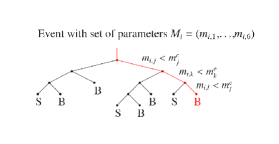
Figure 1: Sketch of a decision tree. An event, described by a parameter set, $M_{i}$ = ($m_{i,1}$,$\ldots$,$m_{i,6}$), undergoes at each node a binary split criterion (passed or failed) on one of its parameters until it ends up in a leaf. This leaf marks it as signal (S) or background (B).

2.2 The training procedure for a single tree

The training or building of a decision tree is the process that finds the appropriate splitting criterion for each node using a training sample, $S$, of events of known type. The training sample is composed of a signal training sample, $S_{1}$, and a background training sample, $S_{2}$, which consist of $N_{1}$ signal and $N_{2}$ background events, respectively. Each event in the training set is characterised by a weighting factor $\omega_{i}$ and a set of input parameters, $M_{i}$. To build a decision tree from such a training sample the following steps are performed:

• The training samples are normalised in such a way that all signal events have the same weight, $\omega_{i}(S_{1})=1/N_{1}$, and all background events have the same weight $\omega_{i}(S_{2})=1/N_{2}$.

• Tree building starts at the root node (top node in Fig. 1), where one finds the variable and split value that provides the best separation of signal and background events. According to this splitting criterion, $S$ is divided into two subsets of events that either pass or fail this criterion. Each subset is fed into a child node where again the cut parameter which separates best signal and background events is determined.

• This procedure is applied recursively until further splitting would not increase the separation, or a preassigned minimum number of events is reached . According to the majority of signal and background events, the last-grown nodes (which are called leaves) are assigned signal (S) or background (B) type, respectively (see Fig. 1).

2.3 Boosting

Single decision trees are sensitive to statistical fluctuations in the training sample, hence a boosting procedure is applied which results in a forest of trees and thus increases the stability of the method. In this procedure, events that got misclassified in the building of the previous tree are multiplied with a boost weight, $\alpha$, thereby getting a higher weight in the training of the next tree. Hence, the boosting is applied to all trees except for the first one. This method is known as AdaBoost or adaptive boost [23]. $\alpha$ is calculated from the fraction of misclassified events in all leaves, $err$:

$$\alpha=\frac{1-err}{err}$$ (1)

After having applied $\alpha$ to each misclassified event, renormalisation of the training samples retains the sum of weights of all events in a decision tree constant.

2.4 BDT settings

In this work we use the BDT method provided by the TMVA package. The decision tree settings are mostly default values, which have been optimised and tested by the TMVA developers. These parameters guarantee a fast training procedure and a stable response of the classifier and are marked with a * in the following.

• The number of trees was chosen to be 200*, which is a compromise between separation performance and processing power. Varying this value in a broad range does not significantly change the presented results.

• The Gini Index* was used as separation type. It calculates the inequality between signal and background distributions for each value to find the best cut. Other separation types were tested and found to achieve similar results.

• Splitting was stopped when the number of events in a node fell below ($N_{1}$ + $N_{2}$) / (10 $\cdot N_{par}^{2}$)*, taking into account the training statistics and the number of training parameters. Typical numbers are between 100 and 1000 for the smallest and largest data set, respectively.

• The number of steps used to scan the parameter space for the best splitting criterion was increased from 20 to 100 to adequately cover training parameters with a large range of values.

3 Training and Evaluation of the BDT method

Having discussed the basic BDT-functioning and details of the growing procedure in the last chapter, this section deals with the training and evaluation of the BDT method. After an introduction of the training parameters used in this work, the properties of the signal- and background training sample are discussed. Finally, tests of the classifiers response are presented.

3.1 Training parameters

The recorded EAS images contain pixels which mainly store photons from the night sky background (NSB). They are removed in an image cleaning procedure [24] for the further image analysis. Only pixels with an intensity of 5 p.e. and a neighbouring pixel with more than 10 p.e. (and vice versa) are kept, thereby just selecting pixels which contain Cherenkov photons originating from the EAS.

To classify the recorded air-shower events as of either signal- or background type, a set of training parameters has been derived using information from the EAS images. The training parameters are based on the Hillas Parameters [10] which are calculated using the second moments of the cleaned shower images. Of these, the width, length, and total intensity (also called image size) of the ellipse are used for classification. Compared to cosmic-ray induced showers, which in general exhibit a rather irregular shape, showers produced by $\gamma$-rays (or electrons) have an elliptical, quite regular structure. The Hillas Parameters inherently store information about the shape of the shower, and can therefore be used to discriminate between cosmic-ray and $\gamma$-ray primaries. Furthermore, an event recorded by multiple telescopes is better constrained. To be independent of the number of participating telescopes (hereafter called multiplicity), the Hillas Parameters of individual telescopes are averaged. The same is true for all the BDT training parameters, presented in the following:

• One type of training parameters is based on the mean reduced scaled width approach introduced by Aharonian et al. [24]. For an image with a given size and reconstructed impact distance the mean expected width for a $\gamma$-ray $\langle W_{i}\rangle$ as obtained from $\gamma$-ray simulations is compared to the measured width $W_{i}$. The Scaled Width for telescope $i$ is then defined as $\mathrm{SCW}_{i}=(W_{i}-\langle W_{i}\rangle)/\sigma_{i}$, with $\sigma_{i}$ being the spread of the expected width. The mean reduced scaled width (MRSW) can then be calculated as the average SCW over all telescopes:

  $$\mathrm{MRSW}=\frac{1}{\displaystyle\sum_{i\in N_{tel}}\omega_{i}}\cdot\displaystyle\sum_{i\in N_{tel}}\left(\mathrm{SCW}_{i}\cdot\omega_{i}\right)\mbox{ ,}$$ (2)

  taking into account the accuracy of the $\gamma$-ray simulations by introducing a weighting factor $\omega_{i}$, defined as $\omega_{i}=\langle W_{i}\rangle^{2}/\sigma_{i}^{2}$.

  Similarly, the mean reduced scaled length (MRSL) is calculated. By comparing the measured width and length of the image with the prediction for an hadronic event , two additional training parameters, the mean reduced scaled width off (MRSWO) and mean reduced scaled length off (MRSLO), are computed.

• Another parameter addresses the different interaction lengths of photons and hadronic cosmic-rays in the atmosphere. It is expressed as the depth of the shower maximum X_max and reconstructed from the recorded shower images. Also this parameter is calculated as a weighted mean value over all participating telescopes.

• Because of their irregular structure, the energy of hadron-induced showers may be reconstructed differently for telescopes seeing the shower from different directions. The $\Delta$E / E parameter, calculated as the averaged spread in energy reconstruction between the triggered telescopes, adds additional separation power to the BDT classification.

For illustration, Fig. 2 shows all training parameter distributions for events with zenith angles around 20^∘ and energies 0.5 TeV $\leq$ E $\leq$ 1.0 TeV.

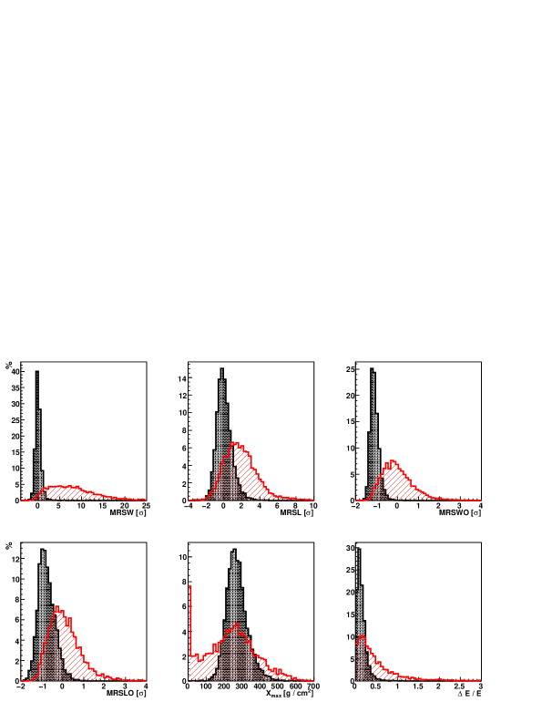
Figure 2: Distribution of the training variables with reconstructed energies between (0.5–1.0) TeV in the zenith angle range (15–25)^∘ for $\gamma$-rays (black) and cosmic-rays (red).

3.2 Training sample

The training set used for building the BDT consists of Monte-Carlo simulations of $\gamma$-rays as signal events, and Off-Events as cosmic ray background. The $\gamma$-rays are simulated as resulting from a point source, at a fixed distance (offset) of 0.5^∘ from the camera centre, and follow an energy distribution dN/dE $\sim$ E^-Γ with index $\Gamma$ = 2.0. Since cosmic-rays reach the earth isotropically, the Off-Events are homogeneously distributed over the field of view of the camera. A cut on the minimum image size of 80 p.e. and the maximum distance between the centre-of-gravity ($COG$) of the Hillas ellipse and the camera centre (to reduce effects of image truncation) was applied to the training sample. This is also referred to as pre-selection and used to exclude poorly reconstructed events from the training process.

3.3 Training

The aim of a BDT classification is a stable $\gamma$/hadron separation over the whole dynamical range of the telescope system, which comprises the accessible energy range as well as the observational conditions (e.g. the zenith angle of the observation). Since the shower shape changes with the primary particle energy and its zenith angle, the distributions of some of the input parameters and consequently the response of the classifier changes. As opposed to the mean reduced scaled parameters which by construction are independent of event energy and zenith angle, the depth of the shower maximum and the uncertainty in the energy estimation do depend on both these quantities.

This characteristic requires a training of the BDT in energy- and zenith angle bands. The energy range accessible for H.E.S.S. (from $\sim$100 GeV to $\sim$100 TeV) was divided into six bands, based on the energy reconstructed assuming a $\gamma$-ray hypothesis, such that for each of seven zenith angle bands (from 0^∘ to 60^∘) the input parameter distributions do not change significantly, and a sufficient number of events for the training process was available. A summary of the training statistics in the energy- and zenith angle bands can be found in Table 1. The decreasing number of training events with increasing energy and/or zenith angle is a direct consequence of the energy spectra of the training sample and the increased energy threshold of the H.E.S.S. system at larger zenith angles.

	0.1 - 0.3	0.3 - 0.5	0.5 - 1.0	1.0 - 2.0	2.0 - 5.0	5.0 - 100.0
0.0 - 15.0	120k/240k	55k/110k	55k/115k	35k/70k	25k/45k	15k/25k
15.0 - 25.0	95k/190k	60k/120k	65k/125k	40k/85k/	30k/55k	15k/35k
25.0 - 35.0	60k/120k	65k/130k	70k/135k	50k/95k	35k/70k	20k/45k
35.0 - 42.5	-/-	75k/150k	75k/155k	55k/115k	45k/95k	35k/65k
42.5 - 47.5	-/-	55k/105k	95k/195k	75k/145k	60k/125k	50k/100k
47.5 - 52.5	-/-	-/-	140k/275k	100k/200k	95k/185k	80k/165k
52.5 - 60.0	-/-	-/-	50k/100k	70k/140k	70k/135k	70k/140k

Table 1: Number of signal- (first value) and background training events (second value) in all trained zenith angle- and energy bands. Events with small energy and large zenith angle cannot be reconstructed since the energy threshold of the H.E.S.S. array increases with zenith angle.

As visible from Fig. 2 all parameters show a more or less pronounced separation power which manifests itself in a different importance of these variables for the building of the BDT. This importance is calculated using the rate of occurrence of a splitting variable during the training procedure, weighted by the squared separation-gain and the number of events in the corresponding nodes [21]. Fig. 3 demonstrates that the relative importance of the training parameters does depend on the energy and zenith angle of the event and that this importance changes from band to band.

While the MRSW parameter is generally the most important classification variable, this is not true for events with energies below a few hundred GeV, since in this energy range hadron- and $\gamma$-initiated showers look similar [25, 26]. Here, the X_max parameter provides better separation, because it carries information about the primary particle interaction length without taking into account the shape of the shower image. Therefore, X_max is uncorrelated with the image shape parameters and an important parameter for the $\gamma$/hadron separation at low energies and large zenith angles.

On the other hand, the spread in event energy reconstruction, $\Delta$E / E, becomes more important for events of high energies, because in this energy range $\gamma$-initiated showers exhibit a rather regular shape, whereas hadron-initiated showers show large fluctuations and therefore a large spread in the energy reconstructed by the participating telescopes.

Also the MRSWO and MRSLO parameters carry additional information about the shower shape. They suffer from the larger hadronic shower fluctuations, but nevertheless contribute to a significant extent to the training procedure.

Beyond the parameters used in this work, additional variables which parametrise the intrinsic image properties (e.g. like those obtained for the 3D Model analysis [11]) are sensitive to different shower properties and could further improve the BDT classification.

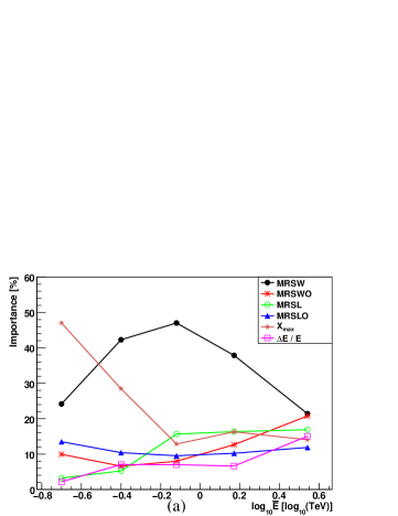
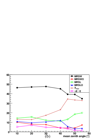
Figure 3: Importance (as defined in the main text) of the training parameters as a function of (a) mean reconstructed energy in the (15–25)^∘ zenith angle band and (b) as a function of mean zenith angle for reconstructed energies between (0.5–1.0) TeV.

3.4 BDT response

After having grown the BDT, the classifier’s response was tested in all zenith angle- and energy bands with an independent test sample of signal- and background events. As an example, Fig. 4 shows the result of the classification of this test sample with the BDT trained in the (0.5–1.0) TeV band with zenith angles (15–25)^∘, demonstrating the excellent classification power of the BDT approach in terms of $\gamma$/hadron separation. However, as explained in the last section, some of the input parameters depend on zenith angle and energy and therefore the $\zeta$ distributions look different from band to band. This later requires zenith- and energy-dependent cuts, to make the $\gamma$/hadron separation independent of the input parameter distributions (Chapter 4.2).

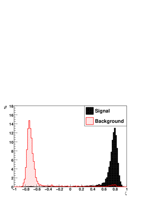
Figure 4: BDT output for events using an independent test sample (same energy and zenith range as in Fig. 2).

4 Systematic studies using H.E.S.S. data

The consistency between data and simulations is one of the key aspects for the analysis of VHE $\gamma$-ray sources. Since observations cover a broad energy range and are performed under various observational conditions (e.g. different zenith angles or telescope configurations), the BDT classification has to be tested under these conditions. For this purpose, we apply the BDT method to H.E.S.S. observations of the Galactic Centre (GC) region performed in 2004 and compare the excess of $\gamma$-rays above the background with the predictions from $\gamma$-ray simulations with similar properties.

4.1 Comparison between simulations and data

The data set used here is a subset of the GC observations [27] and accumulates to a total livetime of 11.4 hours. The data were selected by zenith angle to cover a smaller range of $15^{\circ}\leq\theta\leq 25^{\circ}$, thereby avoiding the mixing of $\gamma$-ray simulations at different zenith angles when comparing the results. The mean offset of the observations is 1^∘. In the following we compare the $\gamma$-ray excess of the GC source HESS J1745–290 to $\gamma$-ray simulations at a fixed zenith- and offset angle of $20^{\circ}$ and 1^∘, respectively. The energy spectrum of HESS J1745–290 follows a power-law in energy with a spectral index of $\Gamma$=2.21 between (0.2–10.0) TeV [28], and the $\gamma$-ray simulations are chosen to match the same spectral shape in this energy range.

The $\zeta$ distributions for events coming from the assumed source region (On-Region) and from seven background control regions (Off-Regions) are shown in Fig. 5, (a). The $\gamma$-ray excess can then be calculated as $\mathrm{N_{\gamma}}=\mathrm{N_{On}}-\alpha\cdot\mathrm{N_{Off}}$, with $\mathrm{N_{On}}$ and $\mathrm{N_{Off}}$ being the number of events from the On-Region and Off-Regions, respectively, and $\alpha$ as normalisation factor which accounts for the different geometrical areas of the On-Region and Off-Regions. The comparison between $\gamma$-ray excess and simulated $\gamma$-rays (Fig. 5, (b)) reveals an excellent agreement and demonstrates that the BDT classifies both type of events in the same way in a broader zenith angle- and energy range.

To illustrate the stability of the BDT classification with respect to different subsets of events, Fig. 6 shows the comparison for events with low energies of 0.2 TeV $\leq$ E $\leq$ 0.4 TeV and for events which were recorded by just two telescopes. These two subsets contain 1/2 and 1/3 of all events, respectively, and are difficult to classify, given the limited separational information for such kind of events. Even for those, the agreement between $\gamma$-ray simulations and $\gamma$-ray excess is obvious and confirms the robustness of the BDT classification.

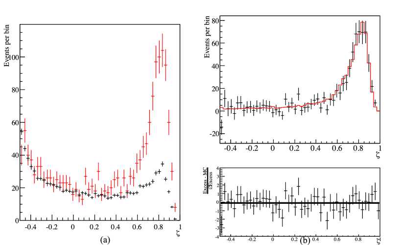
Figure 5: (a): $\zeta$ distribution for events from the On-Region (red) and events from the Off-Regions (black), weighted by $\alpha$, from HESS J1745–290 observations. (b): Comparison between $\gamma$-ray simulations (red curve) and $\gamma$-ray excess, normalised to the number of events in the range ($0\leq\zeta\leq 1$). Also shown are the residua between the two distributions and the result of a fit of a constant, which is compatible with 0 residuum within the statistical errors and has a $\chi^{2}$/ndf of 40/49.

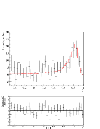
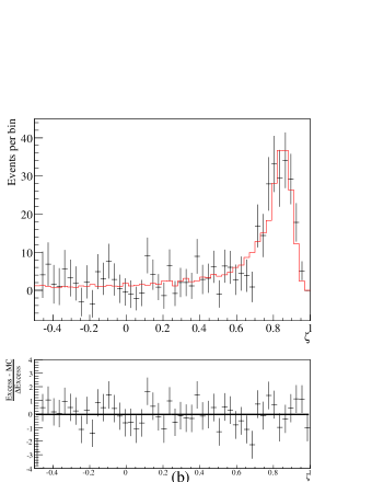
Figure 6: Comparison of $\zeta$ distributions for $\gamma$-ray simulations and $\gamma$-ray excess (a): for events with a multiplicity of 2 and (b): for events with reconstructed energies 0.2 TeV $\leq$ E $\leq$ 0.4 TeV. The lower panel again shows their residua and the result of a fit of a constant. Both fits are compatible with 0 residuum within the statistical errors and have a $\chi^{2}$/ndf of 57/49 and 43/49, respectively.

4.2 Spectral analysis with the BDT method

The last section illustrated that the BDT classification of data and simulations leads to consistent results under variation of different parameters like the covered energy range or the telescope multiplicity of the events. Hence, the BDT classification can be used to select $\gamma$-ray-like events for the spectral analysis of VHE $\gamma$-ray sources.

As aforementioned, the energy- and zenith-dependence of some of the input parameters leads to a zenith- and energy dependent BDT classification. A fixed cut on $\zeta$ would accordingly lead to different cut efficiencies and hence result in a classification which depends on the observational conditions . To circumvent this problem, the independent test sample was used to predict the $\gamma$-efficiency of all possible $\zeta$ cuts in each zenith angle- and energy band. This information was then used to assign a corresponding $\gamma$-efficiency to every $\zeta$ of an event, $\epsilon_{\gamma}(\zeta)$.

In the H.E.S.S. Standard Analysis [24], $\gamma$-ray selection cuts are optimised on MRSW, MRSL, image intensity and $\theta^{2}$ simultaneously to maximise the significance ($\sigma$, defined in [30], Equation (17)). The same optimisation procedure was applied to our analysis, but using $\epsilon_{\gamma}(\zeta)$ instead of MRSW and MRSL. Here we optimised for two different sets of assumed strength and spectral index of the source, namely the $\zeta$ std-cuts (10% of the integrated Crab flux above 200 GeV with a spectral index of $\Gamma$=2.6) and the $\zeta$ hard-cuts (1% of the integrated Crab flux above 200 GeV with a spectral index of $\Gamma$=2.0). Together with the cuts used in the H.E.S.S. Standard Analysis, which are optimised for the same source types, they are summarised and described in Table 2.

(a)

Configuration	$\epsilon_{\gamma}(\zeta)$	$\theta^{2}_{cut}$	Size
	Max	Max	Min
		(degrees2)	(p.e.)
Standard	0.84	0.0125	60
Hard	0.83	0.01	160

(b)

	MRSW	MRSL	$\theta^{2}_{cut}$	Size
Configuration	Max	Max	Max	Min
	$\sigma$	$\sigma$	(deg2)	(p.e.)
Standard	0.9	2.0	0.0125	80
Hard	0.7	2.0	0.01	200

Table 2: (a): Selection cuts optimised for Configuration Standard (strong, steep spectrum sources) and Hard (weak, hard spectrum sources) for the $\zeta$ analysis. (b): Selection cuts optimised for the Standard and Hard Configurations for the H.E.S.S. Standard Analysis [24]. Minimum cuts on MRSW and MRSL of -2.0 are applied in the case of the Standard Analysis.

	0.1 - 0.3	0.3 - 0.5	0.5 - 1.0	1.0 - 2.0	2.0 - 5.0	5.0 - 100.0
0.0 - 15.0	0.28/0.31	0.59/0.61	0.63/0.64	0.52/0.59	0.61/0.62	0.63/0.64
15.0 - 25.0	0.27/0.29	0.56/0.58	0.61/0.63	0.56/0.57	0.56/0.57	0.60/0.61
25.0 - 35.0	0.22/0.25	0.51/0.53	0.59/0.60	0.55/0.57	0.48/0.51	0.54/0.56
35.0 - 42.5	-/-	0.45/0.48	0.58/0.60	0.52/0.53	0.44/0.46	0.43/0.45
42.5 - 47.5	-/-	0.25/0.28	0.54/0.56	0.54/0.56	0.42/0.45	0.39/0.42
47.5 - 52.5	-/-	-/-	0.47/0.50	0.48/0.51	0.36/0.39	0.38/0.41
52.5 - 60.0	-/-	-/-	0.29/0.32	0.46/0.48	0.38/0.40	0.35/0.37

Table 3: $\zeta$ cuts in all zenith angle and energy bands which correspond to an $\epsilon_{\gamma}(\zeta)$ cut of 0.84 ($\zeta$ std-cuts, first value) and 0.83 ($\zeta$ hard-cuts, second value).

The optimised $\zeta$ std-cuts were applied to the HESS J1745–290 data set and a spectrum was extracted. The spectrum obtained for the application of the $\zeta$ std-cuts and the published differential flux [28] are shown in Fig. 7. An excellent agreement between both results further consolidates the applicability of the BDT approach for the analysis of VHE $\gamma$-ray sources. Additional spectral tests with sources of different spectral shape, flux level or source extensions were performed. They show the same agreement between the $\zeta$ std-cuts and the H.E.S.S. Standard Analysis.

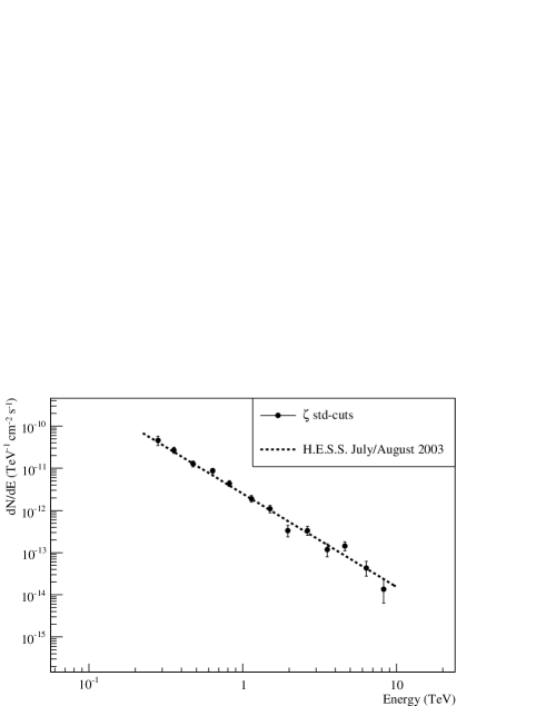
Figure 7: Comparison between the fit to the energy spectrum of HESS J1745–290 for the July/August 2003 data set (dashed line, [28]) and the spectrum obtained with the $\zeta$ std-cuts (filled circles).

5 Performance and Sensitivity

Having shown the applicability of the BDT classification under different observational conditions and for the spectral analysis, the performance and sensitivity of BDT is studied on the basis of $\gamma$-ray simulations and Off-Events.

5.1 Separation power of $\zeta$ cuts

An appropriate parameter to quantify the quality of analysis cuts is the quality factor Q (e.g. [31]), defined as:

$$\mathrm{Q}=\frac{\epsilon_{\gamma}}{\sqrt{\epsilon_{CR}}}\mathrm{,}$$

$$\mathrm{with}\qquad\epsilon_{i}=\frac{\hat{N_{i}}}{N_{i}}\qquad(i=\gamma~{}\mathrm{or~{}CR}),$$

where the cut efficiency $\epsilon_{i}$ is defined as the number of events that pass certain cuts $\hat{N_{i}}$ divided by the number of events before cuts $N_{i}$. Fig. 8 shows the development of Q_ζ / Q_std as a function of zenith angle and energy for the $\zeta$ std- and hard-cuts and the std- and hard-cuts after application of the pre-selection and the image shape selection. The pre-selection consist of the corresponding image size cuts and a cut on the distance between the $COG$ of the shower image and the camera centre to avoid truncated images at the camera edge. The image shape cuts comprehend cuts on $\zeta$ and MRSW, MRSL, respectively (see Table 2 and 3 for further information).

The training in energy- and zenith angle bands leads to a stable improvement in separation power for the BDT method and makes the zenith- and energy-dependent cuts on $\zeta$ well suited for this kind of analysis. Especially at energies below a few hundred GeV and energies above a few TeV the improvement in Q for hard- and std-spectrum sources is remarkable. As a result of the training with $\gamma$-rays simulated at a fixed offset of 0.5^∘, the performance of the $\zeta$ cuts is reduced for events with larger offsets ($\geq 1.5^{\circ}$). However, a training in offset bands resulted in steps in selection efficiency across the field of view and in the description of the camera acceptance, and is therefore not employed.

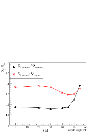
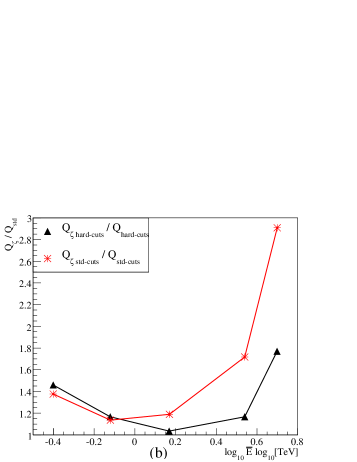
Figure 8: Improvement in Q-factor, defined as Q_ζ / Q_std (Q-factor described in the main text) versus (a): zenith angle and (b): reconstructed energy for the $\zeta$ analysis compared to the H.E.S.S. Standard Analysis. The values for Q are determined using the cut efficiencies for $\gamma$-rays from simulations and background events from off source data in the specific zenith angle and reconstructed energy range.

5.2 Sensitivity of $\zeta$ cuts

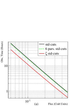
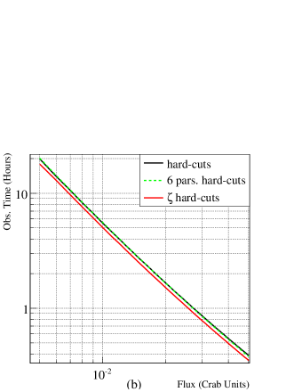
Figure 9: Sensitivity of the H.E.S.S. array for six sets of selection cuts. Shown is the required observation time to detect a point-like $\gamma$-ray source with 5$\sigma$ significance above the background, as a function of the flux of the source with spectral index (a) $\Gamma=2.63$ and (b) $\Gamma=2.0$ at 20^∘ zenith angle and 0.5^∘ offset. Note, that the required observation time is up to 45% and 20% less for the BDT method compared to the H.E.S.S. Standard Analysis for configuration Standard and Hard, respectively. Furthermore, no gain in sensitivity is achieved in the case of the six parameter box cuts optimisation for configuration Hard (black curve is hidden behind the green, dashed curve).

The optimised $\zeta$ cuts (introduced in Section 4.2 and Table 2) are applied to $\gamma$-ray simulations and Off-Events, and their sensitivity for strong, std-spectrum and weak, hard-spectrum sources was calculated. To disentangle the performance improvement due to the information stored in the additional parameters and due to the treatment of non-linear correlations by the BDT method, the sensitivity for optimised box cuts on all training parameters is also shown. These box cuts are a set of one-dimensional cuts on each training parameter which are all optimised simultaneously to obtain the best separation between signal and background.

Fig. 9 illustrates the improved separation power of the $\zeta$ analysis compared to the box cuts applied in the H.E.S.S. Standard Analysis. Shown is the required observation time for a detection (signal with more than 5$\sigma$ above background) of a point source for a range of fluxes, assuming a power-law in energy with a spectral index of $\Gamma=2.63$ as measured for the Crab nebula [24] (Fig. 9, (a)) and for a hard spectrum source with index $\Gamma=2.0$ (Fig. 9, (b)) for the aforementioned sets of selection cuts. Remarkably, the optimised $\zeta$ cuts show the highest sensitivity over a wide range of source strengths. The required observation time for the $\zeta$ analysis is up to  45% and  20% less compared to the H.E.S.S. Standard Analysis, for configuration Standard and Hard, respectively. It is also clear from Fig. 9, that box cuts add just little to the total separation gain, since they ignore non-linear correlations in the six training parameters.

Since the X_max parameter contributes especially at low energies to the classification (see Fig. 3 for comparison), and cuts optimised for hard-spectrum sources tend to reject low-energy events, the performance improvement of the $\zeta$ hard-cuts is only 20% compared to the H.E.S.S. hard-cuts. Nevertheless, the improvement is stable over a wide range of fluxes. One possibility to further improve the BDT performance for hard-spectrum sources is to find the best match between size cut applied to select the training sample (see Section 3.2 for comparison) and size cut optimised for a given source type in an alternating process.

6 Summary and Outlook

IACTs have to deal with a vast number of hadronic cosmic-ray background events. The capability to suppress these against the $\gamma$-rays is one of the aspects which limits the sensitivity of IACTS. In this work the training, testing and evaluation of the BDT method with H.E.S.S. data was presented. The BDT is a multivariate analysis method, which combines the information carried in several classification parameters into one parameter $\zeta$. This parameter describes the likeness of an event to be of hadronic or electromagnetic origin. Observations of the VHE $\gamma$-ray source HESS J1745–290 show a very good agreement between $\zeta$ distribution of the measured $\gamma$-ray excess and the predictions from $\gamma$-ray simulations for a variety of observational conditions. Zenith- and energy-dependent cuts are introduced to account for the zenith and energy-dependent classification of the BDT. Performance tests have shown a dramatically increased separation power for the $\zeta$ analysis compared to the H.E.S.S. Standard Analysis especially for sources with a spectral index compatible with that measured for the Crab nebula.

The systematic studies performed in this work and the achieved classification power demonstrate that a multivariate analysis approach like BDT is well suited for the analysis of $\gamma$-ray data measured with instruments like H.E.S.S.. In near- and mid-term projects like H.E.S.S. II, MAGIC II, CTA and AGIS the accessible energy range of IACTs is extended as the reachable sensitivity increases. Multivariate methods can play a major role for the analysis and particularly for the $\gamma$/hadron separation of upcoming instruments. The majority of the events will be recorded below a 100 GeV, where $\gamma$/hadron separation is increasingly difficult. In this work, performance of parameters such as X_max demonstrate the ability especially for the separation at low energies.

References

- [1] Aharonian, F.A., (H.E.S.S. Collaboration), 2005, Science, 307, 1938
- [2] Aharonian, F.A., (H.E.S.S. Collaboration), 2006a, ApJ, 636, 777
- [3] Hoppe, S., (H.E.S.S. Collaboration), 2007, Proceedings of the 30th International Cosmic Ray Conference, July 3-July 11, 2007, Merida, Mexico, vol. 2, 579-582
- [4] Hinton, J.A. (H.E.S.S. Collaboration), 2004, New Astron. Rev., 48, 331
- [5] Lorenz, E. (MAGIC Collaboration), 2004, New Astron. Rev., 48, 339
- [6] Weekes, T.C. (VERITAS Collaboration), 2002, Astropart. Phys. 17, 221
- [7] Kubo, H. (CANGAROO-III Collaboration), 2004, New Astron. Rev., 48, 323
- [8] Hermann, G., Hofmann, W., Schweizer, T., Teshima, M. (CTA Consortium), 2007, Proceedings of the 30th International Cosmic Ray Conference, July 3-July 11, 2007, Merida, Mexico, vol. 3, 1313-1316
- [9] Fegan, S. and Buckley, J. H. and Bugaev, S. and Funk, S. and Konopelko, A. and Maier, G. and Vassiliev, V. V. and Simulation Studies Working Group and AGIS collaboration, High Energy Astrophysics Division 2008, 10.2806F
- [10] Hillas, A.M., Proceedings of the 19th International Cosmic Ray Conference, August 11-August 23, 1985, La Jolla, USA, vol. 3, 445
- [11] Lemoine-Goumard, M., Degrange, B., Tluczykont, M., 2006, Astropart. Phys., 25, 195
- [12] Breiman, L., 2001, Machine Learning. 45, 1
- [13] Albert, J. (MAGIC Collaboration), 2008, Nucl. Instrum. Meth. A588, 424
- [14] Egberts, K. and Hinton, J.A. (H.E.S.S. Collaboration), 2008, Advances in Space Research, 42, 473F
- [15] Bock, R.K., et al. , 2004, Nucl. Instrum. Meth. A516, 511
- [16] Höcker, A., et al. , TMVA - Toolkit for Multivariate Data Analysis, [physics/0703039v4], 2007
- [17] Roe, B.P., Yang, H.-J., Zhu, J., Liu, Y., Stancu, I and McGregor, G., 2005, Nucl. Instrum. Methods Phys. Res., Sect. A 543, 577
- [18] Yang, H.-J., Roe, B.P. and Zhu, J., 2005, Nucl. Instrum. Methods Phys. Res., Sect A 555, 370
- [19] Benitez, J., 2005, APS Meeting Abstracts, F1028B, 2008
- [20] Bailey, S., et al. , 2007, ApJ, 665, 1246,
- [21] Breiman, L., Friedman, J., Stone, C.J., and Olshen, R.A., Classification and Regression Trees (Wadsworth, Stamford, 1984)
- [22] Bowser-Chao, D., Dzialo, D.L., 1993, Phys. Rev. D 47,1900
- [23] Freund, Y. and Schapire, R.E., 1996, in Machine Learning: Proceedings of the 13th International Conference, edited by Saitta, L. (Morgan Kaufmann, San Francisco, 1996) p.148.
- [24] Aharonian, F.A., Akhperjanian, A.G., Bazer-Bachi, A.R., et al. , 2006b, Astron. & Astrophys., 457, 899-915
- [25] Sobczyńska, D., 2007, J. Phys. G: Nucl. Part. Phys., 34, 2279-2288
- [26] Maier, G and Knapp, J., 2007, Astropart. Phys., 28, 72
- [27] Aharonian, F.A., et al. , 2006c, Phys.Rev.Lett., 97. 221102
- [28] Aharonian, F.A., (H.E.S.S. Collaboration), 2004, Astron. & Astrophys., 425, L13-L17
- [29] Berge, D. and Funk, S. and Hinton, J., 2007, Astron. & Astrophys., 466, 1219-1229
- [30] Li, T.-P. & Ma, Y.-W., 1983, ApJ, 272, 317
- [31] Bugayov, V. V., et al. , 2002, Astropart. Phys., 17, 41