Abstract

We study free particles in a one-dimensional box with combinations of two types of boundary conditions: the Dirichlet condition and a one-parameter family of quasi-Neumann conditions at the two walls. We calculate energy spectra approximately and obtain equations of state having the same (one-dimensional) volume dependence as van der Waals equations of state. The dependence of the equations of state is examined for particles obeying Maxwell-Boltzmann, Bose-Einstein, or Fermi-Dirac statistics. Our results suggest that the deviation from ideal gas may also be realized as finite size effects due to the interaction between the particles and the walls.

1 Introduction

In quantum mechanics, boundary conditions play an important role. A good example is Casimir force [1] predicted in 1948. It is also known that boundary conditions produce force in non-relativistic quantum mechanics [2, 3, 4]. In this paper, we focus on one-dimensional free particles and show that this force leads to equations of state whose one-dimensional volume or length dependence is the same as that of van der Waals equation of state.

Consider a closed box. One may impose the conventional Dirichlet condition on wave functions at the walls of the box. In mathematics, we are, however, permitted to generalize the boundary condition in the context of self-adjoint extensions of Hamiltonian operators [5], where the Dirichlet and Neumann conditions are allowed just as special boundary conditions. Interestingly, it has been pointed out [6] that the generalized boundary conditions can be derived from the vanishing limits of widths of two step functions, which may be realized at, for example, junctions of two semiconductor layers. In this paper, we consider the Dirichlet condition and a class of boundary conditions including the Neumann condition, which we call quasi-Neumann conditions, to find how boundary conditions affect the physical property of the particles in the box. We show that such boundary conditions affect statistical quantities of finite size systems. Note that this effect has no relation with bulk properties of the system in the thermodynamic limit, where the effect that we will obtain disappears.

Specifically, we approximately calculate the spectra of particles in the box by integral approximation and find that the spectra can lead to equations of state having the same dependence on length as van der Waals equation of state. Van der Waals equation was introduced by Johannes Diderik van der Waals in his Ph.D. thesis [7] and has been well-known to describe the behavior of real fluids. Van der Waals-like equations of state were derived from, for example, the Gaussian Markoffian process [8], the intermolecular interaction in classical statistical mechanics [9, 10], the wall-molecular interaction in classical statistical mechanics [11], or the electro-magnetic field [12]. Unlike van der Waals equation of state, our equations of state tend to that for ideal gas in the thermodynamic limit. In finite size system, the quantum boundary effects lead to similar equations of state as the above-mentioned effects. The free particles under the Dirichlet condition [13] and cyclic boundary condition [14] have been studied earlier, and here we consider combinations of the non-trivial boundary conditions and show that they admit equations of state whose length dependence is the same as that of van der Waals equation of state.

This paper is organized as follows. In section 2, we briefly review the method of self-adjoint extensions to characterize the possible boundary conditions. In section 3, we study free particles in a one-dimensional box with the Dirichlet condition at its one wall and a quasi-Neumann condition at the other wall (see the left one of Fig.1). We consider three types of statistics: Maxwell-Boltzmann statistics, Bose-Einstein statistics, and Fermi-Dirac statistics, for which equations of state are obtained. In section 4, we study free particles in a one-dimensional box with identical boundary conditions at its both walls (see the right one of Fig.1), where we assume Maxwell-Boltzmann statistics. In addition, we extend the one-dimensional box with identical quasi-Neumann conditions at both of the walls to a three-dimensional one. In section 5, we summarize our results and discuss the physical meanings on the outcomes.

Figure 1: The energy eigenfunctions and the energy levels in the boxes with different boundary conditions. The solid lines show the eigenfunctions. The height of dashed lines indicates the square root of the energy levels.

2 On self-adjoint extensions of the Hamiltonian

In this section, we give a short review on self-adjoint extensions based on [15]. Consider particles in a one-dimensional box with the length $l$. Each particle is governed by the Hamiltonian,

$$H= -\frac{\hbar^{2}}{2m}\frac{\mathrm{d}^{2}\ }{\mathrm{d}x^{2}},$$ (2.1)

where $x\in[a,b]$ is a coordinate in the box. The Dirichlet conditions may be imposed on a wave function at the walls of the box. In general, infinitely large number of pairs of boundary conditions at both of the walls is permitted as long as the Hamiltonian is self-adjoint in mathematics. It is known that each pair of boundary conditions defines a distinctive wave function and spectrum. Thus, this generalization of boundary conditions has physical meaning.

Let $\textrm{Dom}(H)$ be the domain of the Hamiltonian. If $H$ is a self-adjoint operator, then $\phi_{1},\phi_{2}\in\textrm{Dom}(H)$ must satisfy

$$0 =\int^{b}_{a}\mathrm{d}x\ \phi_{1}^{*}(x)\Big{\{}-\frac{\hbar^{2}}{2m}\frac{\mathrm{d}^{2}}{\mathrm{d}x^{2}}\phi_{2}(x)\Big{\}}-\int^{b}_{a}\mathrm{d}x\Big{\{}-\frac{\hbar^{2}}{2m}\frac{\mathrm{d}^{2}}{\mathrm{d}x^{2}}\phi_{1}(x)\Big{\}}^{*}\phi_{2}(x)$$

$$=-\frac{\hbar^{2}}{2m}\Big{\{}\phi_{1}^{*}(b)\frac{\mathrm{d}\phi_{2}}{\mathrm{d}x}(b)-\frac{\mathrm{d}\phi_{1}^{*}}{\mathrm{d}x}(b)\phi_{2}(b)\Big{\}}+\frac{\hbar^{2}}{2m}\Big{\{}\phi_{1}^{*}(a)\frac{\mathrm{d}\phi_{2}}{\mathrm{d}x}(a)-\frac{\mathrm{d}\phi_{1}^{*}}{\mathrm{d}x}(a)\phi_{2}(a)\Big{\}}.$$ (2.2)

Note that the above equations represent the conservation of the probability current density at both of the walls if $\phi_{1}=\phi_{2}$. We assume that the wall of $x=a$ is disconnected from that of $x=b$, and for example, the cyclic boundary condition is excluded. The disconnected condition implies that each term of the second line of (2.2) must be equal to $0$ independently. We discuss only the boundary at $x=a$, since the boundary condition at $x=b$ can be dealt with similarly.

For convenience, we use $\phi^{\pm}_{i}(x)$ introduced as

$$\phi^{\pm}_{i}(x):=\phi_{i}(x)\pm iL\frac{\mathrm{d}\phi_{i}}{\mathrm{d}x}(x),$$ (2.3)

where $L\in\mathbb{R}$ and $i=1,2$. Note that $L$ has the dimension of length. We can rewrite the condition (2.2) as

$${\phi_{1}^{+}}^{*}(a)\phi_{2}^{+}(a)={\phi_{1}^{-}}^{*}(a)\phi_{2}^{-}(a).$$ (2.4)

The above equation means that the (one-dimensional) Hermite inner product of $\phi_{1}^{+}(a)$ and $\phi_{2}^{+}(a)$ is equal to that of $\phi_{1}^{-}(a)$ and $\phi_{2}^{-}(a)$. Since $\phi_{1}$ and $\phi_{2}$ are arbitrary elements of $\textrm{Dom}(H)$, $\phi^{+}_{i}$ must be connected with $\phi^{-}_{i}$ by a (one-dimensional) unitary transformation specified by $\textrm{Dom}(H)$:

$$e^{i\theta}\phi^{+}_{i}(a) =\phi^{-}_{i}(a).$$ (2.5)

Note that $\textrm{Dom}(H)$ is characterized by the unitary transformation vice versa. This procedure brings the condition of self-adjointness to a simple form:

$$(e^{i\theta}-1)\phi(a)+iL(e^{i\theta}+1)\frac{\mathrm{d}\phi}{\mathrm{d}x}(a) =0.$$ (2.6)

This equation is known as Cheon-Fülöp-Tsutsui boundary equation[16].

We introduce $L_{\theta}:=-L\cot\frac{\theta}{2}$ instead of $L$ and $\theta$, then (2.6) can be written as follows:

$$\phi(l)=L_{\theta}\frac{\mathrm{d}\phi}{\mathrm{d}x}(l).$$ (2.7)

The above equation contains the arbitrary parameter $L_{\theta}$. In mathematics, the Hamiltonian (2.1) is not a bounded operator; therefore it cannot be defined in the entire Hilbert space but a dense subspace of it. The domain of the Hamiltonian cannot be specified uniquely, either. The arbitrary parameter $L_{\theta}$ implies this ununiqueness. In particular, $L_{\theta}=0$ and $L_{\theta}=\infty$ imply the Dirichlet condition and the Neumann condition, respectively. Note that the boundary condition (2.7) has been derived [6] from the limits of two step functions, whose ratio between the heights and widths characterizes $L_{\theta}$

3 The box with the Dirichlet and a quasi-Neumann conditions

In this section, we study the box with the Dirichlet and a quasi-Neumann conditions.

Let $x\in[0,l]$ be a coordinate in the box. We assume that our wave function satisfies the Dirichlet condition at $x=0$ and a boundary condition characterized by $L_{\theta}$ at $x=l$. We restrict ourselves to $|L_{\theta}|>l$ at $x=l$, which is required technically to ensure the validity of our approximation. A class of such boundary conditions includes the Neumann condition, but not the Dirichlet condition; accordingly, we call such a boundary condition a quasi-Neumann condition.

A wave function of each particle is given by

$$\phi(x) =A\sin kx,\hskip 14.22636pt(k\in\mathbb{R}),$$ (3.1)

and its spectrum condition is obtained by

$$\frac{l}{L_{\theta}}=kl\cot kl.$$ (3.2)

Note that the above equation is a transcendental equation; therefore we cannot solve it explicitly.

3.1 Calculation of approximated spectrum

Now we study the equation (3.2) and obtain its approximated solutions. The spectrum condition (3.2) has a solution for each region, $(n-1)\pi<kl<n\pi$, where $n\in\mathbb{N}$. In addition, the solution $kl$ tends to $\pi(n-\frac{1}{2})$ in the limit $n\to\infty$ (see Fig.2). We expand $\cot kl$ as

$$\cot kl=\Big{(}n-\frac{1}{2}\Big{)}\pi-kl+O\Big{[}\Big{(}kl-n\pi+\frac{1}{2}\pi\Big{)}^{3}\Big{]}.$$ (3.3)

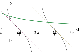
Figure 2: The thin lines represent $y=\cot kl$ and the dashed lines show their linear approximation. The thick line is $y=\frac{l}{L_{\theta}}\frac{1}{kl}$. The crossing points of the thick and thin lines yield the solutions of (3.2). Those of the thick and dashed lines yield the approximation solutions.

For each region, the following inequality is fulfilled:

$$\Big{|}\Big{(}n-\frac{1}{2}\Big{)}\pi-kl\Big{|}<\big{|}\cot kl\big{|}=\Big{|}\frac{l}{L_{\theta}}\frac{1}{kl}\Big{|}.$$ (3.4)

This inequality leads to

$$\Big{|}(n-\frac{1}{2})\pi-kl\Big{|}<\Big{|}\frac{l}{L_{\theta}}\frac{1}{\pi\big{(}n-\frac{1}{2}\big{)}}\Big{|}+O\Bigg{[}\bigg{\{}\frac{l}{L_{\theta}}\frac{1}{\pi\big{(}n-\frac{1}{2}\big{)}}\bigg{\}}^{2}\Bigg{]}.$$ (3.5)

The approximation solution of (3.2) for each region, $(n-1)\pi<kl<n\pi$, is therefore obtained by

$$kl =\pi\Big{(}n-\frac{1}{2}\Big{)}-\frac{l}{\pi L_{\theta}\big{(}n-\frac{1}{2}\big{)}}+O\Bigg{[}\bigg{\{}\frac{l}{L_{\theta}}\frac{1}{\pi\big{(}n-\frac{1}{2}\big{)}}\bigg{\}}^{3}\Bigg{]},$$ (3.6)

where the error term is estimated from (3.5). The solutions lead to energy spectrum of each particle $E_{n}$ as

$$E_{n} =\frac{\kappa}{l^{2}}\bigg{\{}1+\Big{(}\frac{l}{L_{\theta}}\Big{)}^{2}\frac{1}{\pi^{4}\big{(}n-\frac{1}{2}\big{)}^{4}}\bigg{\}}\Big{(}n-\frac{1}{2}\Big{)}^{2}-\frac{\nu}{l}\Bigg{[}1-O\bigg{[}\bigg{\{}\frac{l}{L_{\theta}}\frac{1}{\pi\big{(}n-\frac{1}{2}\big{)}}\bigg{\}}^{2}\bigg{]}\Bigg{]}$$

$$\simeq\frac{\kappa\big{(}n-\frac{1}{2}\big{)}^{2}}{l^{2}}-\frac{\nu}{l},$$ (3.7)

where

$$\kappa :=\frac{\hbar^{2}\pi^{2}}{2m}, \nu :=\frac{\hbar^{2}}{mL_{\theta}},$$ (3.8)

and we ignore the terms of the order $\frac{l}{L_{\theta}}$ by our quasi-Neumann condition.

3.2 Statistical quantity and equation of state

In this section, we calculate statistical quantities and derive equations of state from the spectrum in high temperature region $\frac{\beta\kappa}{l^{2}}<1$. We assume $N$ particles obeying Maxwell-Boltzmann statistics, Bose-Einstein statistics, and Fermi-Dirac statistics.

3.2.1 The case of Maxwell-Boltzmann statistics

Now, we study the case of Maxwell-Boltzmann statistics. By using (A.4), we obtain partition function $Z_{c}$ as follows:

$$Z_{c}= \bigg{\{}\sum_{n=1}^{\infty}\exp(-\beta E_{n})\bigg{\}}^{N}$$

$$= \exp\Big{(}\frac{N\beta\nu}{l}\Big{)}\bigg{\{}\int^{\infty}_{0}\mathrm{d}x\exp\Big{(}-\frac{\beta\kappa}{l^{2}}x^{2}\Big{)}\bigg{\}}^{N}$$

$$= \Big{(}\frac{l}{2}\sqrt{\frac{\pi}{\beta\kappa}}\Big{)}^{N}\exp\Big{(}\frac{N\beta\nu}{l}\Big{)}.$$ (3.9)

Let $p_{c}$ be force acting on the walls of the box. We can, based on statistical mechanics, derive $p_{c}$ from following equation:

$$p_{c}=\frac{1}{\beta Z_{c}}\frac{\mathrm{d}Z_{c}}{\mathrm{d}l}.$$ (3.10)

The equation of state in this case is thus given by

$$\Big{(}p_{c}+\frac{N\nu}{l^{2}}\Big{)}l =\frac{N}{\beta}.$$ (3.11)

The given equation differs from ideal gas law in the term $\frac{N\nu}{l^{2}}$. We refer to this term as a force correction term. Note that (3.11) becomes the equation of state for ideal gas if the wave function satisfies the Neumann condition at $x=l$. This implies that equation of state for ideal gas cannot be derived under a pair of Dirichlet conditions, which will be discussed in section 4.1.

The equation of state (3.11) resembles van der Waals equation of state:

$$\Big{(}p_{\textrm{vdW}}+\frac{N^{2}\nu_{\textrm{vdW}}}{l^{2}}\Big{)}(l-\sigma_{\textrm{vdW}}N)=\frac{N}{\beta}.$$ (3.12)

Van der Waals equation of state is different from ideal gas law in the terms $\frac{N^{2}\nu_{\textrm{vdW}}}{l^{2}}$ and $-\sigma_{\textrm{vdW}}N$. We call the former a force correction term and the latter a length correction term. Van der Waals equation differs from (3.11) in two points. One is that van der Waals equation of state has the length correction term, while (3.11) does not. In section 4, we will derive equations that possess length correction terms, which are however different from van der Waals one. The other is that the force correction term in (3.11) is in proportion to $N$, while that of van der Waals equation of state is in proportion to $N^{2}$; therefore, the force correction term in (3.11) vanishes in the thermodynamic limit $l\to\infty$ under the constant density. This is reasonable because the boundary effects are expected to disappear in the thermodynamic limit, where the property of bulk gas becomes dominant. Our equation is thus meaningful only in finite length systems. We will further discuss this point in the last section.

3.2.2 The cases of Bose-Einstein statistics and Fermi-Dirac statistics

Now, we study the case of quantum statistics. Let bosonic variables be subscripted by $+$ and fermionic variables by $-$.

We express, by using integral approximation (A.4), the particle number $N$ as a function of chemical potential $\mu_{\pm}$ like that:

$$N= \sum^{\infty}_{n=1}\frac{1}{\exp\big{\{}\beta(E_{n}-\mu_{\pm})\big{\}}\mp 1}$$

$$= \pm\frac{l}{2}\sqrt{\frac{\pi}{\beta\kappa}}\textrm{Li}_{\frac{1}{2}}\Big{[}\pm\exp\Big{\{}\beta\big{(}\mu_{\pm}+\frac{\nu}{l}\big{)}\Big{\}}\Big{]},$$ (3.13)

where $\textrm{Li}_{s}(x)$ is polylogarithm function (see Appendix B). Note that the integral approximation of the bosonic case is violated in the region $\beta\big{(}\mu_{+}+\frac{\nu}{l}\big{)}\sim 0$ since the integrand becomes infinity at $\beta\big{(}\mu_{+}+\frac{\nu}{l}\big{)}=0$. We will discuss this case in section 3.3.

Analogously, the force in this case $p_{\pm}$ is obtained by

$$p_{\pm}= -\sum^{\infty}_{n=1}\frac{\mathrm{d}E_{n}}{\mathrm{d}l}\frac{1}{\exp\{\beta(E_{n}-\mu_{-})\}\mp 1}$$

$$= \sum^{\infty}_{n=1}\frac{\frac{2\kappa}{l^{3}}\big{(}n-\frac{1}{2}\big{)}^{2}-\frac{\nu}{l^{2}}}{\exp[\beta(E_{n}-\mu_{-})]\mp 1}$$

$$= \pm\frac{1}{2\beta}\sqrt{\frac{\pi}{\kappa\beta}}\textrm{Li}_{\frac{3}{2}}\Big{[}\pm\exp\Big{\{}\beta(\frac{\nu}{l}+\mu_{\pm})\Big{\}}\Big{]}-\frac{N\nu}{l^{2}}.$$ (3.14)

We can rewrite the equation (3.13) as

$$\frac{\kappa\beta N^{2}}{l^{2}}=\frac{\pi}{4}\bigg{[}\textrm{Li}_{\frac{1}{2}}\big{\{}\pm e^{\beta(\mu_{\pm}+\frac{\nu}{l})}\big{\}}\bigg{]}^{2}.$$ (3.15)

Since $\textrm{Li}_{\frac{1}{2}}(\pm e^{y})$ is a monotone function of $y$, there exists the inverse function; therefore, $\beta\big{(}\mu_{+}+\frac{\nu}{l}\big{)}$ can be regarded as a function of $\frac{\kappa\beta N^{2}}{l^{2}}$. For this reasons, we introduce $R_{\pm}\Big{(}\frac{\kappa\beta N^{2}}{l^{2}}\Big{)}$ by

$$R_{\pm}\Big{(}\frac{\kappa\beta N^{2}}{l^{2}}\Big{)}:=\frac{\textrm{Li}_{\frac{3}{2}}\Big{[}\pm\exp\Big{\{}\beta(\frac{\nu}{l}+\mu_{\pm})\Big{\}}\Big{]}}{\textrm{Li}_{\frac{1}{2}}\Big{[}\pm\exp\Big{\{}\beta(\frac{\nu}{l}+\mu_{\pm})\Big{\}}\Big{]}},$$ (3.16)

whose behavior is shown in Fig. 3.

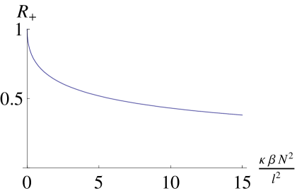
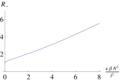
Figure 3: These figures show the behavior of $R_{\pm}$. (Left) Bosons. It shows that $R_{+}$ is a monotonically decreasing function of $\frac{\kappa\beta N^{2}}{l^{2}}$. (Right) Fermions. It shows that $R_{-}$ is a monotonically increasing function of $\frac{\kappa\beta N^{2}}{l^{2}}$. The graphs imply that both $R_{\pm}$ tend to $1$ in the limit $\frac{\kappa\beta N^{2}}{l^{2}}\to 0$.

From the above equation, we can rewrite (3.14) as

$$\Big{(}p_{\pm}+\frac{N\nu}{l^{2}}\Big{)}l=\frac{N}{\beta}R_{\pm}\Big{(}\frac{\kappa\beta N^{2}}{l^{2}}\Big{)}.$$ (3.17)

We regard the above equation as the equation of state in this case, which also has the term, $\frac{N\nu}{l^{2}}$, as is the case for (3.11). We call this term a force correction term as well. In the bosonic case, a similar equation without the force correction term was derived from the cyclic boundary condition in [14]. Note that the equation (3.11) is derived from replacing $R_{\pm}$ with $1$.

3.3 Behavior in the limit $l\to 0$

In the previous section, we calculate the statistics quantities in the high temperature region $\frac{\beta\kappa}{l^{2}}<1$. In this section, we study the behavior of the equations of state in the limit $\beta\to\infty$.

3.3.1 The case of Maxwell-Boltzmann statistics

In the region $\frac{\kappa\beta}{l^{2}}\gg 1$, the integral approximation is not better than first term approximation:

$$Z_{c}=\exp(-\frac{\beta N\kappa}{4l^{2}}+\frac{\beta N\nu}{l}).$$ (3.18)

Then $p_{c}$ is given by

$$\big{(}p_{c}+\frac{N\nu}{l^{2}}\big{)}\ l=\frac{\kappa N}{2l^{2}}.$$ (3.19)

We call the term $\frac{N\nu}{l^{2}}$ a force correction term as well. Note that the term is the same shape as those of (3.11) and (3.17).

3.3.2 The case of Bose-Einstein statistics

In the bosonic case, the integral approximation is not verified in the region $\beta\big{(}\mu_{+}+\frac{\nu}{l}\big{)}\sim 0$, since the integrand of (A.4) diverges at $\beta\big{(}\mu_{+}+\frac{\nu}{l}\big{)}=0$; therefore the second term of the right hand side of (A.4) cannot be neglected. In this region, we use the following approximation:

$$N =\sum_{n=1}^{\infty}\frac{1}{\exp\big{\{}\frac{\beta\kappa}{l^{2}}\big{(}n-\frac{1}{2}\big{)}^{2}-\beta\big{(}\mu_{+}+\frac{\nu}{l}\big{)}\big{\}}-1}$$

$$=\frac{1}{\exp\Big{\{}\frac{\beta\kappa}{4l^{2}}-\beta\big{(}\mu_{+}+\frac{\nu}{l}\big{)}\Big{\}}-1}+\int_{1}^{\infty}\frac{\mathrm{d}x}{\exp\Big{\{}\frac{\beta\kappa}{l^{2}}x^{2}-\beta\big{(}\mu_{+}+\frac{\nu}{l}\big{)}\Big{\}}-1}.$$ (3.20)

An upper bound of the integral term is given by

$$\int_{1}^{\infty}\frac{dx}{\exp\big{\{}\frac{\beta\kappa}{l^{2}}x^{2}-\beta\big{(}\mu_{+}+\frac{\nu}{l}\big{)}\big{\}}-1}< \int^{\infty}_{1}\frac{dx}{\frac{\beta\kappa}{l^{2}}x^{2}-\beta\big{(}\mu_{+}+\frac{\nu}{l}\big{)}-1}$$

$$< \frac{l^{2}}{\beta\kappa}.$$ (3.21)

If $\frac{N}{2}\gg\frac{l^{2}}{\beta\kappa}$, the first term of the second line of (3.20) is much bigger than the integral term. In other words, the average number of the particles in the ground state is much bigger than that in the excited states. Bose-Einstein condensation therefore happens in that region. Note that the condition, $\frac{N}{2}\gg\frac{l^{2}}{\beta\kappa}$, is independent of the boundary parameter $L_{\theta}$. In this region, we can neglect the integral term of (3.20); therefore the equation of state is given by as follows:

$$\big{(}p_{+}+\frac{N\nu}{l^{2}}\big{)}\ l=\frac{\kappa N}{2l^{2}}.$$ (3.22)

The above equation is identical to (3.19) based on Maxwell-Boltzmann statistics.

3.3.3 The case of Fermi-Dirac statistics

In the fermionic case, the equation of state (3.17) is still valid in the limit of $\beta\to\infty$. From appendix B, the asymptotic behavior of $R_{-}(z)$ in the limit of $z\to\infty$ is

$$R_{-}(z)\to \frac{2}{3}z.$$ (3.23)

The equation of state thus tends to

$$\big{(}p_{-}+\frac{N\nu}{l^{2}}\big{)}\ l=\frac{2\kappa N^{3}}{3l^{2}}.$$ (3.24)

We also call the term $\frac{N\nu}{l^{2}}$ a force correction term. Note that the force correction term is the same shape as those of (3.11), (3.17), (3.19), and (3.20).

4 Pairs of identical boundary conditions

We have studied the statistical quantities of the system in the box with the Dirichlet condition and a quasi-Neumann condition in the previous section. In this section, we assume pairs of identical boundary conditions: a pair of the Dirichlet conditions and a pair of identical quasi-Neumann conditions. In addition, we extend the one-dimensional box with a pair of quasi-Neumann conditions to a three-dimensional box. We consider particles obeying Maxwell-Boltzmann statistics since the quantum statistics cases are hard to study by using the method developed in section 3.

4.1 One-dimensional box with the Dirichlet condition

In section 3.2.1, we have shown that the equation of state under Maxwell-Boltzmann statistics with the pair of the Dirichlet condition and the Neumann condition is identical to that for ideal gas. In this section, we show that the equation of state of the pair of the Dirichlet conditions is different from that for ideal gas.

We impose the Dirichlet condition at the walls of the box. Let $E_{n}$ be energy of each particle given by

$$E_{n}=\frac{\kappa n^{2}}{l^{2}},$$ (4.1)

where $n\in\mathbb{N}$. By using (A.8), we obtain partition function $Z^{DD}$ as follows:

$$Z^{DD} =\big{\{}\sum_{n=1}^{\infty}\exp(-\beta E_{n})\big{\}}^{N}$$

$$=\Big{\{}\int^{\infty}_{0}\mathrm{d}x\exp\big{(}-\frac{\beta\kappa}{l^{2}}x^{2}\big{)}-\frac{1}{2}\Big{\}}^{N}$$

$$=\Big{(}\frac{l}{2}\sqrt{\frac{\pi}{\kappa\beta}}-\frac{1}{2}\Big{)}^{N}.$$ (4.2)

Let $p^{DD}$ be the force acting on the wall. The equation of state in this case is thus given by

$$p^{DD}\ \bigg{(}l-\sqrt{\frac{\beta\kappa}{\pi}}\bigg{)}=\frac{N}{\beta}.$$ (4.3)

We call the term $-\sqrt{\frac{\beta\kappa}{\pi}}$ a length correction term. The above equation of state is clearly different from ideal gas law, which is derived from classical statistical mechanics; therefore quantum effect is responsible for this difference.

Tsutsui et al. have studied a one-dimensional box with a partition at the center of the box [2, 3]. They imposed the Dirichlet conditions on wave functions at the walls of the box. They also imposed the Dirichlet condition at one side of the partition and the Neumann condition at the other side of the partition. It was shown that the partition is, in high temperature limit $\beta\to 0$, subjected to force $\Delta p$ given by

$$\Delta p=\frac{N}{l^{2}}\sqrt{\frac{\kappa}{\beta\pi}},$$ (4.4)

where $l$ is the length of each half of the box.

Below, we derive $\Delta p$ from the equations of state (3.11) and (4.3). In the high temperature limit, the length correction term is smaller than $l$; therefore we approximately rewrite $p^{DD}$ as follows:

$$p^{DD} =\frac{N}{l\beta}\frac{1}{1-\frac{1}{l}\sqrt{\frac{\beta\kappa}{\pi}}}$$

$$\sim\frac{N}{l\beta}+\frac{N}{l^{2}}\sqrt{\frac{\kappa}{\beta\pi}}$$

$$=p^{DN}+\Delta p,$$ (4.5)

where $p^{DN}$ is the force of Maxwell-Boltzmann particles in the box with a pair of the Dirichlet condition and the Neumann condition. Since the difference of the forces $p^{DD}-p^{DN}$ is given by $\Delta p$, our results agree with that of [2, 3] in the high temperature limit.

4.2 One-dimensional box with a quasi-Neumann Condition

In this section, we study particles in the box with a quasi-Neumann condition. Let $x\in[-\frac{l}{2},\frac{l}{2}]$ be a coordinate in the box. We assume identical boundary conditions at the walls. In accordance with [18], the boundary conditions at $x=\frac{l}{2}$ and $x=-\frac{l}{2}$ are characterized by the boundary parameters $L_{\theta}$ and $-L_{\theta}$, respectively. The sign change of the boundary parameter is caused by reversing the direction where the particles collide on the wall. The wave functions are given by three the types:

$$\phi =\cos k_{1}x$$ (4.6)

$$\phi =\sin k_{2}x$$ (4.7)

$$\phi =\cosh k_{3}x,$$ (4.8)

where $k_{1}$, $k_{2}$, and $k_{3}$ satisfy following quantization conditions:

$$-\frac{l}{L_{\theta}} =k_{1}l\tan\frac{k_{1}l}{2}$$ (4.9)

$$\frac{l}{L_{\theta}} =k_{2}l\cot\frac{k_{2}l}{2}$$ (4.10)

$$\frac{l}{L_{\theta}} =k_{3}l\tanh\frac{k_{3}l}{2}.$$ (4.11)

The approximation (3.3) and

$$\tan x =x-n\pi+O\big{[}(x-n\pi)^{3}\big{]}$$ (4.12)

$$\tanh x =x+O\big{[}x^{3}\big{]}$$ (4.13)

lead to energy spectrum of each particle as

$$E_{n}=\frac{\kappa(n-1)^{2}}{l^{2}}-\frac{2\nu}{l},$$ (4.14)

where $n\in\mathbb{N}$. By using equation (A.8), we obtain partition function $Z^{NN}$ as follows:

$$Z^{NN} =\big{\{}\sum_{n=1}^{\infty}\exp(-\beta E_{n})\big{\}}^{N}$$

$$=\exp\Big{(}\frac{2N\nu\beta}{l}\Big{)}\Big{\{}\int^{\infty}_{0}\mathrm{d}x\exp\big{(}-\frac{\beta\kappa}{l^{2}}x^{2}\big{)}+\frac{1}{2}\Big{\}}^{N}$$

$$=\exp\Big{(}\frac{2N\nu\beta}{l}\Big{)}\Big{(}\frac{l}{2}\sqrt{\frac{\pi}{\kappa\beta}}+\frac{1}{2}\Big{)}^{N}.$$ (4.15)

Let force acting on the wall be $p^{NN}$. An equation of state in this case is given by

$$\Big{(}p^{NN}+\frac{2N\nu}{l^{2}}\Big{)}\bigg{(}l+\sqrt{\frac{\beta\kappa}{\pi}}\bigg{)}=\frac{N}{\beta}.$$ (4.16)

We call the term $\frac{2N\nu}{l^{2}}$ a force correction term and the term $\sqrt{\frac{\beta\kappa}{\pi}}$ a length correction term. Note that $\nu=0$ implies the Neumann condition. Let $p^{N}$ be force under the pair of the Neumann conditions, the equation of state is given by

$$p^{N}\bigg{(}l+\sqrt{\frac{\beta\kappa}{\pi}}\bigg{)}=\frac{N}{\beta}.$$ (4.17)

The above equation is different from the equation of the pair of the Dirichlet conditions (4.3).

4.3 Three-dimensional box with a quasi-Neumann condition

Here, we study a three-dimensional box with a quasi-Neumann condition at the wall of box. Let $(x,y,z)$ be a three-dimensional Cartesian coordinate. Consider a cuboid box whose median point is the origin of the coordinate. Let its sides be parallel to the coordinate axes. We introduce $l_{x},l_{y}$, and $l_{z}$ as the lengths of the sides. As is the previous section, we impose identical boundary conditions at the walls of the box: the boundary condition at $x=\frac{l_{x}}{2}$, $y=\frac{l_{y}}{2}$, and $z=\frac{l_{z}}{2}$ are characterized by $L_{\theta}$ and the boundary condition at $x=-\frac{l_{x}}{2}$, $y=-\frac{l_{y}}{2}$, and $z=-\frac{l_{z}}{2}$ are characterized by $-L_{\theta}$. We introduce quantum numbers for $x$, $y$, and $z$ directions as $n_{x}$, $n_{y}$, $n_{z}\in\mathbb{N}$, which characterize energy of a particle, $E_{n_{x},n_{y},n_{z}}$, as

$$E_{n_{x},n_{y},n_{z}}=\kappa\bigg{\{}\frac{(n_{x}-1)^{2}}{l_{x}^{2}}+\frac{(n_{y}-1)^{2}}{l_{y}^{2}}+\frac{(n_{z}-1)^{2}}{l_{z}^{2}}\bigg{\}}-2\nu\bigg{(}\frac{1}{l_{x}}+\frac{1}{l_{y}}+\frac{1}{l_{z}}\Big{)}.$$ (4.18)

The energy implies that force is different by the directions. We introduce $p_{x}$ as force of the $x$ direction, the equation of state is given by

$$\bigg{(}p_{x}+\frac{2N\nu S_{x}}{V^{2}}\bigg{)}\bigg{(}V+S_{x}\sqrt{\frac{\kappa\beta}{\pi}}\bigg{)}=\frac{N}{\beta},$$ (4.19)

where $S_{x}=l_{y}l_{z}$ and $V=l_{x}S_{x}$. The force of the other directions is obtained by the same calculation. Note that the terms showing the aeolotropic behavior of pressure vanish in the thermodynamic limit $V\to\infty$ under the constant density condition, $\frac{N}{V}=$ constant. The equation of state (4.19) thus predicts no aeolotropic bulk gas but shows the dependence of boundary effects on the scale of the system.

5 Conclusion and Discussion

We studied free particles in a closed box whose boundary conditions are generalized by self-adjoint extensions of the Hamiltonian. We solved the energy spectrum conditions approximately and obtained the equations of state from the energy spectra by integral approximation. Note that our results are significant primarily for finite size systems since the boundary effects disappear in the thermodynamic limit; therefore, our equations of state do not describe the bulk properties of free particles at the thermodynamic limit.

We assume three different combinations of the boundary conditions. First, we considered the one-dimensional box with the Dirichlet condition and a quasi-Neumann condition. We assumed three types of statistics: Maxwell-Boltzmann, Bose-Einstein, and Fermi-Dirac statistics, and obtained the equations of state (3.11) and (3.17) and evaluated the behavior of the equations in the limit $l\to 0$, arriving at (3.19), (3.22), and (3.24). Although these five equations are different in statistics and in the region of $l$, they share the same force correction terms. The common force correction terms have the same dependence on length as that of van der Waals equation. The force correction terms are dependent on the boundary parameter, whereas other terms are independent.

Second, we studied Maxwell-Boltzmann particles under the Dirichlet condition at both of the walls. We found that the equation of state (4.3) is no longer that of ideal gas due to the length correction term in (4.3), which is different from that of van der Waals equation of state (3.12). It has been studied in [2, 3] that there is a difference between two pressures, one of which obtained under the pair of the Dirichlet conditions and the other evaluated under the pair of the Dirichlet and the Neumann conditions. The equations of state of (3.11) and (4.3) lead to the high temperature limit of the pressure difference (4.4), which is an increasing function of temperature and vanishes in the thermodynamic limit.

Third, we studied particles obeying Maxwell-Boltzmann statistics under a quasi Neumann condition at both of the walls. We obtained the equation of state (4.16), which has both the length correction term and the force correction term. The strength of the force correction term in this case is twice of that of the pair of the Dirichlet condition and a quasi Neumann condition. The length correction term in this case is similar to that of the pair of the Dirichlet conditions except for its sign. Note that the equation of the pair of the Neumann conditions (4.17) is different from that of the pair of the Dirichlet conditions.

These three results clearly show that boundary conditions can yield force correction terms that have inverse square dependence on the length, analogously to van der Waals equation. However, the force correction term in van der Waals equation and those of our equations are different in particle number dependence. Our equations of state are influenced by boundary effects which vanish in the thermodynamic limit, and hence they are meaningful only in the finite length system. In the case of van der Waals equation, the order $N^{2}$ is regarded as the number of the inter-molecular interactions, which is $N(N-1)\sim N^{2}$ since the $N$ particles interact with each other. On the other hand, the force correction term of the pair of the Dirichlet condition and a quasi Neumann condition is in proportion to $N$ and that of the pair of quasi Neumann conditions is twice of that of the pair of the Dirichlet condition and a quasi Neumann condition. There is no force correction term in the equation of state of the pair of the Dirichlet conditions. Interestingly, the product of the particle number and the number of the walls of a quasi Neumann condition equals the dependence of the particle number of the force correction terms in our model. This implies that the particle number dependence can be interpreted as the number of the interactions, as in the case with van der Waals equation.

We also briefly touched upon the three-dimensional box with a quasi-Neumann condition. The obtained equation of state (4.19) is a three-dimensional extension of the one-dimensional equation (4.16) and we find that the three-dimensional equation possesses the same property of the one-dimensional equation, confirming that boundary effects can appear in three dimensions, too. Finally, we mention that generalized boundary conditions have been used for effective descriptions of rapidly varying potentials at small scales, which are approximately represented by the vanishing limit of widths of step functions [6, 19, 20]. There, the boundary condition (2.7) and parameter $L_{\theta}$ are derived from such limits of two step functions [6]. These circumstances may appear, for instance, at junctions of two semiconductor layers and, if so, our boundary effects may actually be observed experimentally.

6 Acknowledgements

The author would like to thank Prof. I. Tsutsui and Dr. Y. Abe, Dr. T. Ichikawa, T. Sasaki and H. Imazato for useful comments.

Appendix A On approximation

In this appendix, we give a brief account of integral approximation of the sum of series. For all $n\in\mathbb{Z}$, $f(x)$ can be expanded as

$$f(x)=\sum_{k=0}^{\infty}\frac{1}{k!}\Big{(}x-n-\frac{1}{2}\Big{)}^{k}f^{(k)}(n+\frac{1}{2}),$$ (A.1)

where $x\in(n,n+1)$. We obtain

$$\int_{0}^{\infty}f(x)dx=\sum_{k=0}^{\infty}\frac{1}{(2k+1)!}\frac{1}{2^{2k}}T_{2k},$$ (A.2)

where

$$T_{k}:=\sum_{n=0}^{\infty}f^{(k)}(n+\frac{1}{2}).$$ (A.3)

We apply the above equation to $f^{(2k)}(x)$ and eliminate the differential term by successive iteration, then we obtain the following series expansion:

$$\int_{0}^{\infty}f(x)dx=\sum_{n=1}^{\infty}a_{2n-1}f^{(2n-1)}(0)+\sum_{n=0}^{\infty}f(n+\frac{1}{2}),$$ (A.4)

where

$$\kappa_{k}:= \frac{1}{k!}\frac{1}{2^{k}}$$

$$a_{2k-1}= 2\kappa_{2k+1}-\sum_{n=1}^{k-1}2\kappa_{2n+1}a_{2(k-n)-1}.$$ (A.5)

The coefficient $a_{2k-1}$ tends to $0$ rapidly in the limit $k\to\infty$. In addition, $f(x)=F(\sqrt{\alpha}x)$ in our system; therefore

$$f^{(n)}(0)\sim O[\alpha^{\frac{n}{2}}].$$ (A.6)

From the above equations, then we can neglect the sum of the first term of the right hand side of (A.4) if $\alpha<1$.

Now, we show a similar formula to (A.4). Let f(x) expand as follows:

$$f(x)=\sum_{k=0}^{\infty}\frac{1}{k!}\Big{(}x-n\Big{)}^{k}f^{(k)}(n).$$ (A.7)

We define $S_{k}:=\sum_{n=0}^{\infty}f^{(k)}(n)$ and repeat the above discussion, then the following equation is obtained:

$$\int_{0}^{\infty}f(x)dx =\sum_{k=0}^{\infty}\frac{1}{(k+1)!}\frac{1}{2^{k+1}}f^{(k)}(0)+\sum_{k=1}^{\infty}\frac{1}{(2k+1)!}\frac{1}{2^{2k}}\sum_{n=0}^{\infty}f^{(2k)}(n)$$

$$=\sum_{n=1}^{\infty}f(n)+\sum_{n=0}^{\infty}b_{n}f^{(n)}(0),$$ (A.8)

where

$$b_{0} =\frac{1}{2}$$

$$b_{2k} =\frac{1}{2}a_{2k-1}$$

$$b_{2k-1} =a_{2k-1}+\kappa_{2k}-\sum_{n=1}^{k-1}\kappa_{2n}a_{2(k-n)-1}.$$ (A.9)

Appendix B On polylogarithm

The polylogarithm[22], $\textrm{Li}_{s}(z)$, is defined in $|z|<1$ as follows:

$$\textrm{Li}_{s}(z)=\sum_{k=1}^{\infty}\frac{z^{k}}{k^{s}}.$$ (B.1)

In $|z|>1$, it is defined by analytical continuation of the above equation. It satisfies the following formulae:

$$\textrm{Li}_{s}(-z)+\textrm{Li}_{s}(z) =2^{1-s}\textrm{Li}_{s}(z^{2})$$ (B.2)

$$\lim_{\textrm{Re}(\mu)\to\infty}\textrm{Li}_{s}(e^{\mu}) =-\frac{\mu^{s}}{\Gamma(s+1)};$$ (B.3)

therefore we obtain the asymptotic behavior of them:

$$\textrm{Li}_{\frac{1}{2}}\big{\{}-\exp(z)\big{\}} \to-2\sqrt{\frac{z}{\pi}}$$ (B.4)

$$\textrm{Li}_{\frac{3}{2}}\big{\{}-\exp\big{(}z\big{)}\big{\}} \to-\frac{4z}{3}\sqrt{\frac{z}{\pi}}.$$ (B.5)

We can express $\textrm{Li}_{\frac{1}{2}}(\pm e^{y})$ and $\textrm{Li}_{\frac{3}{2}}(\pm e^{y})$ in integral forms as

$$\textrm{Li}_{\frac{1}{2}}(\pm e^{y}) =\int^{\infty}_{0}\frac{2\ \mathrm{d}x}{\pm\exp[\pi x^{2}-y]-1}$$ (B.6)

$$\textrm{Li}_{\frac{3}{2}}(\pm e^{y}) =\int^{\infty}_{0}\frac{4\pi x^{2}\ \mathrm{d}x}{\pm\exp[\pi x^{2}-y]-1}.$$ (B.7)

The above equations imply that $\textrm{Li}_{\frac{1}{2}}(\pm e^{y})$ and $\textrm{Li}_{\frac{3}{2}}(\pm e^{y})$ are monotone functions because of the integrands are monotone functions of $y$.

References

- [1] H. B. G. Casimir, Proc. Kon. Nederl. Akad. Wet. 51(1948)793
- [2] T. Flp, H. Miyazaki, I. Tsutsui, Mod. Phys. Lett. A18 (2003) 2863
- [3] T. Flp, I. Tsutsui, J. Phys. A: Math. Theor. 40 (2007) 4585
- [4] T. Flp, I. Tsutsui, J. Phys. A: Math. Theor. 42 (2009) 475301
- [5] Methods of Modern Mathematical Physics II: Fourier Analysis, Self Adjointness, M. Read, B. Simon, Academic Press, New York, San Francisco, London.
- [6] T. Fülöp, T. Cheon, I. Tsutsui, Phys. Rev. A66 (2002) 052102.
- [7] J. D. van der Waals, ”Over de Continuiteit van den Gasmen Vloeistoftoestand”. Thesis, Leiden (1873)
- [8] M. Kac, G. E. Uhlenbeck, P.C. Hemmer, J. Math. Phys. 4 (1963) 216
- [9] E. M. Lifshitz, L. P. Pitaevskii, Statistical Physics Part 1, Pergramon press, 3rd ed. (1959) 232
- [10] Byung Chan Eu, Kyunil Rah, Phys. Rev. E 63 (2001) 031203
- [11] D. E. Sullivan, Phys. Rev. B 20 (1979) 3991
- [12] I. E. Dzyaloshinskii, E. M. Lifshitz, L. P. Pitaevskii, Sov. Phys. Usp. 4 (1961) 153
- [13] S. Grossmann, M. Holthaus, Z. Phys. B 97 (1995) 319
- [14] D. J. Toms, J. Phys. A: Math. Gen. 39 (2006) 713
- [15] I. Tsutsui, T. Fülöp, T. Cheon, Ann. Phys. 294 (2001) 1
- [16] I. Tsutsui, T. Flp, T. Cheon, J. Phys. A: Math. Gen. 36 (2003) 275
- [17] B. M. Levitan, I. S. Sargsjan, Introduction to spectral theory, Providence, Rhode Island (1975) 9
- [18] I. Tsutsui, T. Fülöp, T. Cheon, J. Math. Phys. 42 (2001) 5687.
- [19] T. Shigehara, H. Mizoguchi, T. Mishima, T. Cheon, IEICE Trans. Fund. Elec. Comm. Comp. Sci. E82-A (1999) 1708
- [20] T. Cheon, T. Shigehara, K. Takayanagi, J. Phys. Soc. Jpn, 69 (2000) 345
- [21] P. eba, Czech. J. Phys. B36 (1986) 667
- [22] D. Wood, Technical Report 15, University of Kent, Computing Laboratory, University of Kent, Canterbury, UK, June 1992.
- [23] B. W. Smith, M. Monthioux, D. E. Luzzi, Nature 396 (1998) 323