Enhanced imaging of microcalcifications in digital breast tomosynthesis through improved image-reconstruction algorithms

Abstract

PURPOSE:
We develop a practical, iterative algorithm for image-reconstruction in under-sampled tomographic systems, such as digital breast tomosynthesis (DBT).

METHOD:
The algorithm controls image regularity by minimizing the image total $p$-variation (TpV), a function that reduces to the total variation when $p=1.0$ or the image roughness when $p=2.0$. Constraints on the image, such as image positivity and estimated projection-data tolerance, are enforced by projection onto convex sets (POCS). The fact that the tomographic system is under-sampled translates to the mathematical property that many widely varied resultant volumes may correspond to a given data tolerance. Thus the application of image regularity serves two purposes: (1) reduction of the number of resultant volumes out of those allowed by fixing the data tolerance, finding the minimum image TpV for fixed data tolerance, and (2) traditional regularization, sacrificing data fidelity for higher image regularity. The present algorithm allows for this dual role of image regularity in under-sampled tomography.

RESULTS:
The proposed image-reconstruction algorithm is applied to three clinical DBT data sets. The DBT cases include one with microcalcifications and two with masses.

CONCLUSION:
Results indicate that there may be a substantial advantage in using the present image-reconstruction algorithm for microcalcification imaging.

I Introduction

Digital breast tomosynthesis (DBT) is an emerging X-ray imaging modality that aims at improving the effectiveness of mammographic screening without an increase in radiation dose. DBT provides partial tomographic information that aids in reducing the impact of overlapping tissue structures on tumor detection Niklason et al. (1997); III and Godfrey (2003). A key component of the system is the image-reconstruction (or synthesis) algorithm. Data acquired in DBT are far from sufficient for “exact” tomographic image-reconstruction, which limit the effectiveness of single-pass algorithms. Such algorithms are generally derived from algorithms that assume complete tomographic data, and they generally introduce artifacts in the DBT images. Nonetheless, one-pass algorithms such as filtered back-projection (FBP), modified FBP and matrix-inversion methods are employed to produce images. A thorough investigation on DBT image reconstruction algorithms Wu et al. (2004); Karellas and Giger (2004); Zhang et al. (2006), showed that iterative algorithms present many advantages over one-pass algorithms. Reasons for this include (1) iterative algorithms generally put milder assumptions on the “missing” data; most FBP algorithms set missing views to zero – which is an impossibility for projection imaging, and (2) iterative algorithms allow for physical constraints to be easily incorporated such as physical borders of the object, and valid range for X-ray attenuation values. Here, we investigate iterative image-reconstruction in DBT based on image total p-variation (TpV) minimization Chartrand (2007); Sidky et al. (2007).

Investigation of existing iterative algorithms applied to DBT has been performed in Refs. Wu et al. (2004); Karellas and Giger (2004); Zhang et al. (2006). These references cover the principal iterative algorithms used in tomographic image-reconstruction, demonstrating their performance on various imaging features pertaining to DBT. Maximum likelihood (ML) methods and variations on the algebraic reconstruction technique (ART) are studied. These iterative algorithms, however, may not be ideally suited to image-reconstruction in DBT. Generally speaking, iterative algorithms have been designed to work efficiently for scanning systems where the projection data are complete, or nearly complete, but of low quality. For example, in most nuclear medicine imaging systems, the collected projection data is usually fully sampled allowing for “exact” inversion, at least theoretically, but the data are often corrupted by high levels of noise. As a result, an iterative algorithm is often employed. DBT scanning is challenging for image-reconstruction algorithms in a different way. The data are of high quality (low noise), but they are radically incomplete. This incompleteness means that there may be many, very different, candidate attenuation distributions that agree with the available data. In fact, the recent interest in compressive sensing Candès et al. (2006a, b), poses the extreme limit of the latter situation: namely, can one obtain exact image-reconstruction from “perfect” quality data that is under-sampled. In this article, we adapt an algorithm Sidky and Pan (2008), which we have developed for investigating compressive sensing in tomographic image-reconstruction, to the DBT scanning system.

Iterative image-reconstruction algorithms aim to minimize an objective function that combines a data fidelity term and a regularization term. The overall picture is that there is a trade-off between the two terms. When the weight on the regularization term is small the resulting image yields data that is “close” to the available data, but it may contain conspicuous artifacts due to noise or other inconsistencies in the data. When the weight on the regularization term is large, the resulting image will be regularized at the expense of faithfulness to the data. This picture applies to the scanning situation where the data are complete, but of low quality. For incomplete data scans, however, this trade-off picture is too simple. One of the basic properties of a tomographic system that collects incomplete projection data is that there is not a unique image that corresponds to the available projection data. As a result, regularization of the image takes on two roles: (1) selection of a unique image among those that agree with the projection data, and (2) the traditional role where the image is regularized while relaxing consistency with the available data. In the first role, the image regularization is lowered while the image is constrained to a given data agreement. In the second role the data constraint on the image is relaxed allowing for further minimization of the image regularization.

In our previous work, the image reconstruction algorithm employed projection onto convex sets (POCS) to enforce a data consistency constraint as well as other physical constraints such as positivity, and steepest descent was used to minimize the regularization term. There was an adaptive element introduced to control the relative step-sizes of the POCS and steepest descent components of the algorithm, hence the algorithm is called adaptive steepest descent - POCS (ASD-POCS) Sidky and Pan (2008). The ASD-POCS algorithm allows for the separation of the two roles for the regularizer in tomographic image-reconstruction from incomplete projection-data. Our previous work was focused on compressive sensing in tomography and was restricted to $\ell_{1}$-based regularizers, and algorithm efficiency was a secondary concern.

In this article, we break-up the pieces of the ASD-POCS algorithm, and reassemble them into a simplified, practical image-reconstruction algorithm that we apply to DBT. The practical aspect refers to the fact that we aim to obtain useful images within 10-20 iterations, and the simplification of the algorithm refers to a reduction in the number of algorithm parameters to only those that have a significant impact on the image within the first few iteration steps. Although we provide a specific algorithm here, we do not claim that it is optimal; there are likely many ways to reassemble the ASD-POCS algorithm pieces that yield useful tomographic images. As a result, we refer to ASD-POCS as a framework instead of a single algorithm. Few quantitative comparisons are made as such detailed comparisons make sense only when a particular scan geometry, set of reconstruction parameters, and image regularizer is selected. The various images are shown to reveal the effect of various algorithm parameters on the reconstructed images.

The remainder of the paper is organized as follows: Sec. II describes the general data model for iterative image-reconstruction in X-ray based tomography, Sec. III motivates the need for a new type of iterative algorithm for incomplete scanning configurations such as DBT, Sec. IV presents an image-reconstruction algorithm for DBT derived within the ASD-POCS framework, and Sec. V demonstrates the image-reconstruction algorithm with actual DBT case data that contains both microcalcifications and masses.

II System model and image-reconstruction

We describe the system model for X-ray tomography for which we develop the image-reconstruction algorithm from the ASD-POCS framework. On the one hand, the presentation is quite general in that the image-reconstruction algorithm can be applied to a wide class of linear system models. On the other hand, many aspects of the algorithm implementation are quite specific. For example, the representation of the imaging volume, i.e. voxel shape, is designed with the DBT scan in mind. In this introductory section, we aim the discussion toward general X-ray tomography, but we specify the particular geometry and implementations used here to obtain the DBT results.

Figure 1: Configuration of the digital breast tomosynthesis system. The coordinate system, whose origin lies on the center of rotation for the X-ray source, is also indicated. The front view shows a schematic including the compression paddle. The walls of this paddle are visible in many of the projections.

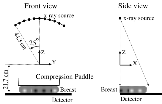
DBT has undergone much development recently, and there are two main configurations being pursued. Most companies working on DBT are developing variations of a swinging X-ray source, while XCounter is proposing a linear X-ray movement system. The common denominator for DBT systems is that projection data is acquired over a limited number of angles with respect to a full, circular tomographic scan as acquired in CT. For the present study we perform volume reconstruction from data acquired by a DBT prototype developed at Massachusetts General Hospital in collaboration with General Electric Healthcare. The scanner configuration and properties are specified in Ref. Wu et al. (2004), but we re-iterate the geometric configuration here. As shown in Fig. 1, the breast is compressed to a thickness of 3-8 cm on a carbon-fiber tray protecting the fixed, flat-panel detector. The X-ray source is moved on an arc, centered on point $h=21.7$ cm above the detector, and with radius $R=44.3$ cm. The detector is composed of an array of 1800x2304 detector bins with width 100 microns, and is physical dimensions are $W=180.0$ mm $\times$ $L=230.4$ mm. The number of projections is 11, and they are approximately equally spaced along the 50^∘ arc. In the article we use the term ”in-plane” to refer to $xy$-planes, parallel to the detector, and the term ”depth” to refer to the $z$-direction, perpendicular to the detector.

The data at each detector bin can be approximately related to the line integral of the breast X-ray attenuation-map:

$$g(s,u,v)=\int d\ell f(\vec{r}_{0}(s)+\ell\hat{\theta}(s,u,v)),$$ (1)

where the source position follows

$$\vec{r}_{0}(s)=(0,R\sin{s},R\cos{s}),$$ (2)

and the detector bin locations are described by

$$\vec{d}(u,v)=(u,v-L/2,-h).$$ (3)

The unit vector $\hat{\theta}(s,u,v)$ points from X-ray source to detector bin:

$$\hat{\theta}(s,u,v)=\frac{\vec{d}(u,v)-\vec{r}_{0}(s)}{|\vec{d}(u,v)-\vec{r}_{0}(s)|}.$$ (4)

The data model in Eq. (1) involves integration of the continuous object. But for the majority of iterative image-reconstruction algorithms further approximation is necessary, because these algorithms generally apply to only finite linear systems and as a result the imaging volume must have a finite representation.

For the discussion below this imaging equation is converted to a discrete, linear system:

$$M\vec{f}=\tilde{g}.$$ (5)

The image vector, $\vec{f}$, is a finite set of coefficients specifying the particular combination of basis elements, which in this case are voxels. The available set of projection data, $\tilde{g}$, will in general have a different size than the set of image basis elements. The system matrix $M$ approximates the continuous line integration of Eq. (1). The particular form of $M$ depends on how the integration approximation is formulated and on the choice of image basis functions. For the current work, we employ the standard voxel representation of the imaging volume. The choice of voxel dimensions typical in DBT are asymmetric. For specifying the voxel size, the in-plane resolution is taken to be the detector resolution – in this case 100 microns. The depth resolution, however, is about 10-fold lower. In previous work, the voxel size has been taken as 0.1x0.1x1.0 mm³ Wu et al. (2003, 2004), and we do the same. With this choice of voxel dimension, the imaging volume is composed of 30 to 80 slices arranged parallel to the detector and within each slice there are the same number of voxels as detector bins. For the reconstructions presented in the results, the slice number is fixed at 60.

Before going on to specify the exact form of $M$, we take an aside here to discuss projection data incompleteness. The important point about incomplete scanning data, is that there may be many attenuation distributions that agree with the available projection data, or equivalently, that solve Eq. (5). There are two aspects to the data incompleteness: the number of measurements may be less than the number of unknowns, and the system matrix $M$ may be ill-conditioned. DBT suffers from both types of incompleteness. For the present imaging volume the number of unknown voxel values is 110,880,000, while the number of measured rays for the 11-projection DBT data set is 22,351,560. Thus, based on vector dimensions alone, the DBT system is under-sampled by a factor of 5. A way to think about the stability issue is that there may be many attenuation distributions that approximately solve Eq. (5), or more precisely, given a “small”, positive number $\delta$ many images may satisfy the following inequality:

$$\|M\vec{f}-\tilde{g}\|\leq\delta.$$ (6)

For example, if the number of views is increased by a factor of 10 the DBT system may still suffer from the second kind of data incompleteness because the geometrical arrangement of the measured rays may not be optimal for tomographic image-reconstruction. The incompleteness in the DBT scan means small changes in the reconstruction algorithm may have a large effect on the reconstructed images, and the data incompleteness plays an integral role in the algorithm design of Sec. IV.

The projection matrix $M$ employed here is ray-driven, meaning that the individual rays of the projection are first identified and the contribution of image voxels to the individual rays is computed. For each ray in the projection data set, the intersection of that ray with the mid-plane of each slice is computed. The contribution of the ray-integral for a particular slice is obtained by linearly interpolating the neighboring four voxel values within the slice and multiplying the result by the ray path-length through the slice. Each of the slice contributions are subsequently summed to yield the ray integral. In practice, the size of $M$ is enormous. For the present set-up using 60 slices, $M$ has on the order of $10^{15}$ elements. Typically, $M$ is computed on-the-fly which is quite efficient for projection, because at most 240 voxels contribute to each ray integration.

The above discussion specifies the form of the linear system that we seek to solve. In the next section, the need for a new algorithm is motivated.

III Iterative algorithms and DBT image-reconstruction

As we have discussed above, the DBT scanning system yields incomplete data for tomographic image-reconstruction. Most of the commonly used iterative algorithms are based on an optimization problem containing two terms: (1) data error $\delta$, the difference between the available data and the estimated projection data based on the current image estimate, and (2) an image regularity penalty, some function, $R(\cdot)$, of the image that increases with “roughness” or some other undesirable property of the image. The function $R(\cdot)$ can take many forms, such as image total variation or squared voxel differences, the roughness. The data-error, can also take different functional forms. The usual optimization problem minimizes an objective function that is the sum of these two terms combined with a parameter to control the strength of the regularization.

Figure 2: Diagram of in the $R,\delta$-plane comparing possible images for an under-sampled versus a completely-sampled tomographic system. The dark region represents images of the latter case. For completely-sampled systems, a unique image minimizes the data error, $\delta$, hence only one value of $R$ is possible. For under-sampled systems, the lightly shaded region, many possible candidate volumes correspond to the situation of minimum $\delta$. The circled point has significance for compressive sensing, if $R$ is the $\ell_{1}$-norm or image total-variation. The two curves represent generic behavior of standard iterative algorithms for the case of no regularization (solid curve), and with regularization (dashed curve).

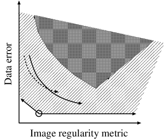
The sketch in Fig. 2 illustrates the difference between the present DBT scanning system and tomographic systems with complete but low-quality data. Each point on the $R,\delta$-plane represents an image estimate, or possibly multiple image estimates corresponding to the same data-error and image-regularity measure. The dark-shaded region is indicative of completely-sampled, high-noise system. Lower values of the data-error generally leads to worse image-regularity. Minimizing the data-error leads to a very small set (possibly only one) of image estimates that is generally very noisy. Hence, rarely is the image at the bottom of the dark region, minimum $\delta$ ever sought. Instead, a regularity penalty is introduced in to the objective function, and an image along the left-edge of the dark region is obtained, yielding a smoother image with greater data-error. The light-shaded region represents possible image estimates for an under-sampled, low-noise scanning system, such as DBT. The achievable data-errors are much lower because the data are of higher quality and there is generally less inconsistency when the projection data are under-sampled. As the system is under-sampled, there is not a unique image that minimizes the data error. In the schematic, there may be many images with different values of the regularity measure that have the minimum data error. As a result, for an effective image reconstruction algorithm for undersampled tomographic systems, it is desirable to be able to independently control the data error and regularity of the image estimates.

The curves shown in Fig. 2 sketch possible trajectories of standard iterative methods applied to the under-sampled system. The solid curve represents iterations from a generic algorithm that minimizes data error. If the algorithm is initialized with a uniform image, as is often done, the image regularity measure starts at low values and the data error is high. As the iterations progress, the image estimate migrates down and to the right. Reduced data error is obtained, generally, at the expense of worse image regularity. If a penalty term is introduced, one might obtain the dashed curve. The image estimates will have lower values of $R(\cdot)$, but the data-error will decrease more slowly. As a result, iterative algorithms that include a penalty term of fixed strength may not be the most efficient for under-sampled tomographic image-reconstruction.

The ASD-POCS algorithm, we developed in Ref. Sidky and Pan (2008), was designed for compressive-sensing tomographic image-reconstruction. Specifically, it was designed to solve the following constrained minimization

$$\vec{f}^{*}=\text{argmin}\;R(\vec{f}),$$ (7)

subject to the constraints

$$\left|M\vec{f}-\tilde{g}\right|^{2}\leq\epsilon^{2},$$ (8)

$$\vec{f}\geq 0.$$

For the compressive sensing application, the ASD-POCS algorithm uses the image total variation (TV) as the regularity measure $R(\cdot)$. The minimum TV image is sought for a fixed data error $\epsilon$ ($\delta\leq\epsilon$). Minimum TV images have the sparsest gradient magnitude images, which is an assumption that applies well to underlying images that are piecewise constant. In particular, one of the goals of ASD-POCS is to closely approximate the image with minimum data error and minimum TV, indicated by the circle in Fig. 2. More generally, the ASD-POCS algorithm can be used to search the lightly-shaded region of the figure, and the function $R(\cdot)$ may take other forms.

IV a practical image-reconstruction algorithm using the ASD-POCS framework

Although the ASD-POCS algorithm is effective at finding a close approximation to the solution of the constrained minimization Eqs. (7) and (8), it may take hundreds to thousands of iterations to obtain a satisfactory solution. Keeping practicality in mind, we assemble an algorithm within the ASD-POCS framework that is more efficient and employs fewer algorithm parameters.

The ASD-POCS algorithm solves the constrained minimization problem by employing POCS to enforce the convex constraints on the image combined with steepest descent to reduce the $R(\cdot)$ objective function. One modification is that we include a line search on the steepest descent portion of the algorithm. The line search ensures that the steepest-descent steps actually reduce the objective $R(\cdot)$ from the first iteration on. This change reduces artifacts in the early iterations (this is not done in the original ASD-POCS algorithm, because it may sacrifice the ability of the algorithm to yield a good approximation to the constrained-minimization problem). Another important modification is reducing the number of control parameters for the adaptation of the step-sizes. The previous version of ASD-POCS had 6 control parameters, which served its purpose of obtaining a good approximate solution to the constrained minimization problem. Because the optimization problem, Eqs. (7) and (8), was being solved, the 6 control parameters affect only the “path” of the image estimate but the final image could be regarded as depending only on the single parameter $\epsilon$ in the constraint. For the present case, where we intend to truncate the iteration well short of convergence, the reconstructed image has to be viewed as a function of the algorithm parameters and $\epsilon$. Having to explore the impact of seven parameters negates the advantage of truncating the iteration early.

We present the new version of the ASD-POCS algorithm in the form of a pseudo-code and abbreviate the notation where possible. The symbol $:=$ means assignment, meaning that the result on the right-hand side gets assigned to the variable on the left-hand side; image-space variables have a vector sign, e.g. $\vec{f}$, and a hat is used if the vector has unit length; data-space variables are denoted by a tilde, e.g. $\tilde{g}$. The number of measured rays, length of $\tilde{g}$, is $N_{d}$. The vector $\vec{M}_{i}$ is the row of the system matrix that yields the $i$th data element. The function $P$ enforces lower and upper bounds on an image estimate: $P(\vec{f},a,b)$ yields the image $\vec{f}^{\prime}$ with components

$$f^{\prime}_{i}=\begin{cases}a&f_{i}<a\\ f_{i}&a\leq f_{i}\leq b\\ b&f_{i}>b\end{cases}.$$

The function $R(\cdot)$ is the image regularity measure.

The pseudo-code is:

1:	$\beta:=1.0;\;N_{\text{iter}}=10$
2:	$ng:=5$
3:	$r_{\text{max}}:=1.0$
4:	$\gamma_{\text{red}}:=0.8$
5:	$\vec{f}:=0$
6:	for $i=1,N_{\text{iter}}$ do				main loop (POCS/descent loop)
7:		$\vec{f}_{0}:=\vec{f}$
8:		for $j=1,N_{d}$ do: $\vec{f}:=\vec{f}+\beta\vec{M}_{j}\frac{g_{j}-\vec{M}_{j}\cdot\vec{f}}{\vec{M}_{j}\cdot\vec{M}_{j}}$				ART
9:		$\vec{f}:=P(\vec{f},0,f_{\text{max}})$			enforce bounding constraints
10:		$\vec{f}_{\text{res}}:=\vec{f}$
11:		$dp:=|\vec{f}-\vec{f}_{0}|$
12:		$\vec{f}_{0}:=\vec{f}$
13:		for $j=1,ng$ do			steepest descent loop
14:			$R_{0}:=R(\vec{f})$
15:			$\vec{df}:=\nabla_{\vec{f}}R(\vec{f})$
16:			$\hat{df}:=\vec{df}/|\vec{df}|$
17:			$\vec{f}^{\prime}:=\vec{f}-dp*\hat{df}$
18:			$\vec{f}^{\prime}:=P(\vec{f}^{\prime},0,f_{\text{max}})$
19:			$\gamma:=1.0$
20:			while $R(\vec{f}^{\prime})>R_{0}$ do		projected line search
21:				$\gamma:=\gamma*\gamma_{\text{red}}$
22:				$\vec{f}^{\prime}:=\vec{f}-\gamma dp*\hat{df}$
23:				$\vec{f}^{\prime}:=P(\vec{f}^{\prime},0,f_{\text{max}})$
24:			end while
25:			$\vec{f}:=\vec{f}^{\prime}$
26:		end for
27:		$dg:=|\vec{f}^{\prime}-\vec{f}_{0}|$
28:		if $dg>r_{\text{max}}*dp$ then $\vec{f}:=r_{\text{max}}\frac{dp}{dg}(\vec{f}^{\prime}-\vec{f}_{0})+\vec{f}_{0}$
29:	end for
30:	return $\vec{f}_{\text{res}}$

The primary controls of the ASD-POCS algorithm are the parameters $\beta$ and $N_{\text{iter}}$ on line 1. As $\beta$ is lowered from a value of 1.0, the image-estimate regularity is decreased, and as the $N_{\text{iter}}$ increases the image-estimate data-error is reduced. In terms of the $R,\delta$ diagram of Fig. 2, $\beta$ is a horizontal control and $N_{\text{iter}}$ is a vertical control.

For readers interested in the reasoning behind this version of the ASD-POCS algorithm, the remainder of this section provides a detailed explanation of the algorithm roughly in the order of the pseudo-code, starting with line 8: Reduction of the data error is accomplished through ART at line 8, and positivity is enforced by the projection at line 9. For the results below, we do not enforce an image upper bound, $f_{\text{max}}=\infty$, because there is little impact. In general, the size of the image-change due to POCS, $dp$ in the pseudo-code, is large relative to the progress made by steepest descent on $R(\cdot)$ especially when we require that the objective function be reduced with each steepest descent step. Thus, the algorithm is designed to make as much progress as possible, in terms of maximizing $dg$, on steepest descent of $R(\cdot)$. First, multiple gradient descent steps are taken with the loop starting at line 13. We found that $ng=5$ loops makes decent progress. Many more loops than that yields diminishing returns. This parameter is not critical, and we leave it fixed at 5. Second, the projected line search at lines 19-24 is slightly unusual in that it is designed to maximize the steepest descent step-size, $dg$, while not increasing the objective function $R(\cdot)$. Thus, the line search algorithm will in general not find the minimum of $R(\cdot)$ along the image-change direction $\hat{df}$ as is normally done with line searches. A relatively large line-search-reduction parameter, $\gamma_{\text{red}}:=0.8$, is chosen so that, again, $dg$ will be maximal. Furthermore, the initial guess for the line-search step-size of $dp$, at line 17, is very aggressive. Choosing $\gamma_{\text{red}}:=0.8$ is not critical for the results and we leave it fixed, but it does impact algorithm efficiency. The image estimate resulting from the steepest descent section will respect positivity because of the projections at lines 18 and 23.

The adaptive element of this algorithm occurs at line 28. The reasoning goes that as long as the change in the image due to POCS $dp$ is not less than $dg$, each iteration of the outer loop will make net progress in reducing the data error. In the early iterations, when $dp$ is large, the steepest descent on $R(\cdot)$ is allowed to take large steps, thereby quickly reducing the image regularity measure. At later steps $dg$ is constrained to lower values so that data error is not increased. We include the ratio parameter $r_{\text{max}}=1.0$ even though it’s not used here. For applications with very high quality data and when it is feasible to take many more iterations such as a hundred or more, it may be desirable to set $r_{\text{max}}<1.0$ in order to make more progress in reducing data error. If algorithm efficiency is of no concern, then the reader is referred to our previous ASD-POCS algorithm Sidky and Pan (2008), where precise control over the data-error tolerance $\epsilon$ is afforded. For the present algorithm the tolerance parameter $\epsilon$ is traded for iteration number, which ends up being the parameter that controls data error. In order to control image regularity, normally the steepest-descent step would be reduced or increased. But, as it is important to maximize $dg$ for efficiency, we instead control the POCS step-size. This is effectively controlled by the relaxation parameter $\beta$. It is set to 1.0 in the pseudo-code, but we vary this control parameter in a range of 0.1 to 1.0, below. To summarize, the controls of the algorithm are: iteration number, more iterations reduce data error; and $\beta$, lower $\beta$ reduces $R(\cdot)$.

The final image $\vec{f}_{\text{res}}$ is considered to be the one after the POCS steps, at line 10, and this is the one shown in the present results. But we point out that there is a non-negligible difference between this image and the image estimate following the steepest descent Sidky et al. (2006). We point out also, that we do not claim this algorithm is optimal in any sense. We regard ASD-POCS as a framework for generating specific image-reconstruction algorithms. The adaptive control step, line 28, can be done differently. For example, in our previous algorithm in Ref. Sidky and Pan (2008) the data error of the current image estimate is compared against a pre-set data tolerance $\epsilon$. Also, different convex constraints on the image function can be included in $P$, i.e, different bounds or support constraints.

Before going on to the results, we mention a few points about algorithm efficiency. As written above, the pseudo-code is quite inefficient for the early iterations of the steepest-descent line-search. At line 20 it is likely that $R(\vec{f}^{\prime})>>R_{0}$, so it may be desirable to include extra logic that allows much smaller values of $\gamma_{\text{red}}$ when this is the case, switching back to the larger value when $R(\vec{f}^{\prime})$ is near $R_{0}$. The pseudo-code above is presented above with simplicity in mind, so there is no doubt that other such tricks could substantially improve run time. Computation of the gradient of $R(\vec{f})$ in line 15 is easily implemented on commodity graphics hardware Sidky and Pan (Lindau, Germany 2007).

V application to DBT projection data

In this section, we employ the practical ASD-POCS image-reconstruction algorithm to clinical DBT projection data obtained on the GE-MGH instrument. In the following, results of the image reconstruction are displayed for cases containing microcalcifications and masses. It will be evident that the ASD-POCS algorithm can have a significant impact on microcalcification imaging.

V.1 DBT projection data

Figure 3: (Left) A single projection for the case containing a uniform mass. (Right) Cropped view used for reconstruction.

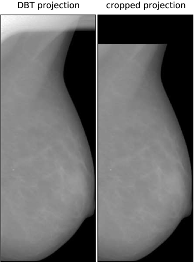
As stated earlier, the scan consists of 11 projection views acquired over a 50^∘ arc. The geometry of the system is shown in Fig. 1. An example projection from this system is shown in Fig. 3 for a view offset at 25^∘. Note that, for this view, a fin from the compression paddle appears in the projection. For such views we truncate the projections to eliminate rays passing through this fin, because the fin is not in the reconstruction volume. Doing so reduces artifacts at the edge of the reconstruction volume, and it allows us to demonstrate convergence properties of the ASD-POCS algorithm.

V.2 Form of the ASD-POCS objective function and algorithm parameters

The ASD-POCS algorithm, presented in Sec. IV, was shown with a generic objective function. For DBT image-reconstruction, here, we employ a total p-variation (TpV) norm of the image as the objective. The TpV norm of the image, written in terms of image voxel values $f_{i,j,k}$, is

$$\left\|\vec{f}\right\|_{TpV}=\sum_{i,j,k}\Delta_{i,j,k}^{p},$$ (9)

where

$$\Delta_{i,j,k}=\sqrt{(f_{i,j,k}-f_{i-1,j,k})^{2}+(f_{i,j,k}-f_{i,j-1,k})^{2}+(f_{i,j,k}-f_{i,j,k-1})^{2}+s}.$$ (10)

The parameter $s$ is set to $10^{-6}$, here, and it is needed to ensure that the TpV norm is differentiable with respect to voxel value when $p\leq 1.0$. Because $\Delta_{i,j,k}$ involves a backward difference, the summations in Eq. (9) start at the second voxel number. For the images reconstructed below, we take the values of $p$ to be 0.8, 1.0 and 2.0 . The case of $p=0.8$, results in a non-convex norm, and it may have some advantage for image-reconstruction from incomplete projection data Chartrand (2007); Sidky et al. (2007). When $p=1.0$, the TpV-norm reduces to the standard TV-norm which is convex, and when $p=2.0$ TpV becomes a quadratic, roughness measure, which is commonly used as a penalty term for iterative image-reconstruction. It is demonstrated in the results that the value of $p$ has a significant impact on image quality for DBT.

The image array used in the reconstruction consists of 60 slices, 1 mm thick, stacked parallel to the detector. The in-plane voxel width is 0.1 mm, matching the detector resolution. The in-plane extent of the slices vary with each case because of breast-size variation (the volume dimensions are given with each case, below). The imaging volume is unusual in that the voxels are 10 times longer in depth than their transverse width. The limited angular range of the DBT scan does not readily yield much information on depth variations, hence the thick slices. Two interesting algorithm aspects that we do not explore here are (1) increasing depth resolution in the imaging volume and (2) employing spatial differencing for the TpV-norm. Thinner slices may yield improved depth resolution when used in combination with the TpV-norm for values $p\leq 1.0$. There are also preliminary indications that using spatial differencing in Eq. (10), where the voxel differences in each dimension are divided by the corresponding voxel length, may improve depth resolution. We have found that these factors make little difference for the ASD-POCS algorithm when run in the 10-20 iteration range. But increasing depth resolution or employing spatial differencing may yield significantly different images that solve the optimization problem, Eqs. (7) and (8).

For completeness, we provide the expression for the voxel-gradient of the objective function, Eq. (9), which is needed for the ASD-POCS algorithm at line 15 of the pseudo-code. The $i,j,k^{th}$ component of the gradient is given by:

$$\partial\left\|\vec{f}\right\|_{TpV}/\partial f_{i,j,k}= \Delta_{i,j,k}^{p-2}(3f_{i,j,k}-f_{i-1,j,k}-f_{i,j-1,k}-f_{i,j,k-1})+$$

$$\Delta_{i+1,j,k}^{p-2}(f_{i,j,k}-f_{i+1,j,k})+\Delta_{i,j+1,k}^{p-2}(f_{i,j,k}-f_{i,j+1,k})+\Delta_{i,j,k+1}^{p-2}(f_{i,j,k}-f_{i,j,k+1}).$$ (11)

Note that this expression applies only to interior voxels. At the edges of the imaging volume the terms that involve voxels outside the imaging volume should be eliminated.

V.3 Reconstructed images

We demonstrate the ASD-POCS algorithm by investigating image-reconstruction on three sets of DBT clinical data: one that contains microcalcifications and two cases that have masses. For each case, images from a basic EM implementation are also shown. The EM implementation used is given by the following update equation

$$\vec{f}^{(k+1)}=\vec{f}^{(k)}\cdot\frac{M^{T}\cdot\left(\tilde{g}/(M\cdot\vec{f}^{(k)})\right)}{M^{T}\cdot\tilde{I}},$$ (12)

where $\tilde{I}$ is a data vector with every element set to 1, $k$ is the iteration number, and the image estimate at $k=0$ is initialized to 1’s in each voxel. We stress that the EM images are shown only to give a rough idea on the performance of current algorithms. Furthermore, the goal of this article is not to claim that ASD-POCS yields “better” images, because that is a task dependent issue. Although the results do seem to indicate a potential advantage for microcalcification imaging. The aim here, however, is mainly to demonstrate the image-regularization controls of the ASD-POCS algorithm. Using these controls, the images can be optimized for different tasks in future work.

Each of the three cases, below, are reconstructed in the same way, meaning the same sets of algorithm parameters are used. The exceptions to this are that the image volume dimensions and the projection data cropping are slightly different for each case. For the EM results images are shown at 5,10, and 20 iterations, as iteration number is really the main control for regularization. For ASD-POCS, the objection function parameter $p$ is set to 0.8, 1.0, and 2.0; lower values of $p$ tend to sharpen edges. The relaxation factor $\beta$ takes on values of 1.0, 0.5, and 0.1; smaller $\beta$, in general, allows for ASD-POCS to achieve lower values of the TpV objective. Images for ASD-POCS are also shown for 5, 10, and 20 iterations. As will be seen, there is surprisingly little change in the reconstructed images for these iteration numbers. In each of the image sets, a 2D ROI is displayed that shows either microcalcifications or a mass, depending on the case.

V.4 Case 1: microcalcifications

Figure 4: ROI reconstructions of the data set containing microcalcifications by the EM algorithm at (left) 5, (middle) 10, and (right) 20 iterations. The gray scale window is [0.30,0.65].

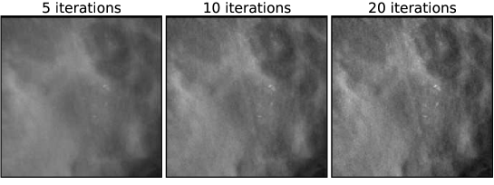
A set of EM images for the first case is shown in Fig. 4, and the corresponding ASD-POCS images are shown in Figs. 5, 6, and 7. A striking feature of the ASD-POCS reconstructions is the prominence of the microcalcifications. Lower values of $p$ accentuate these small features better than large $p$-values. Even for $p=2.0$, the visibility of the microcalcifications is comparable to that of the EM results. The differences in microcalcification contrast can be seen quantitatively in the profiles shown in Fig. 8. These profiles are plotted along depth and transverse lines that intersect with a single microcalcification. We point out that while lower $\beta$ increases regularization strength in ASD-POCS and lower iteration number increases regularization strength for EM, there is no direct correspondence between the two parameters; the chosen iteration numbers for the EM profiles are selected only for reference. Interestingly, there seems to be little change in the ASD-POCS image for iteration numbers 5-20, which obviously has some practical implication.

Figure 5: ROI reconstructions of the data set containing a microcalcifications by the ASD-POCS framework with $\beta=1.0$. The gray scale window is held fixed, and is the same as that of the EM results, [0.30,0.65].

Figure 6: Same as Fig. 5 except $\beta=0.5$.

Figure 7: Same as Fig. 5 except $\beta=0.1$.

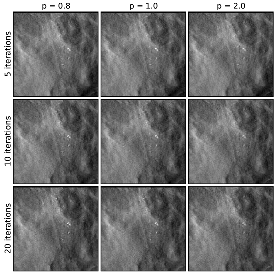
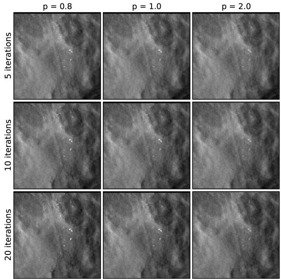
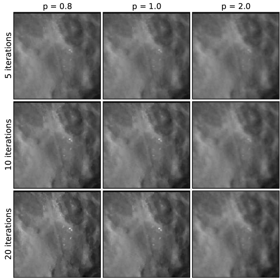
From the profiles and slice images, it is clear that lower $p$ in ASD-POCS enhances microcalcification contrast substantially, leaving one to wonder if there is any advantage to larger $p$-values. While lower $p$-values appear to be advantageous, there is also an impact of $p$-value on the image background. The ROIs displayed in Figs. 5, 6, and 7 are shown in a large enough region to obtain some sense of the difference in background. Again, we are trying, here, to only give some intuition on the parameter-space $(p,\beta)$ dependence of the ASD-POCS algorithm. Optimal values of $p$ and $\beta$ for particular tasks, such as microcalcification detection by human observers, need to be investigated in separate studies. Another important factor that affects selection of $p$ and $\beta$ is data quality. Lower values of $p$, for example, may be robust against detector noise, but may be also more sensitive to inconsistency due to patient motion.

Figure 8: Profiles, centered on a microcalcification, through reconstructed images for different values of $p$ and $\beta$. Also shown are results by the EM algorithm. The comparison of EM at different iteration number does not necessarily have any relation to the ASD-POCS results at different $\beta$. (Top) Transverse profiles along the $x$-direction. (Bottom) Depth profiles in the $z$-direction. The fact that microcalcification have a greater width in the depth profiles is likely to inherent blurring in the DBT system.

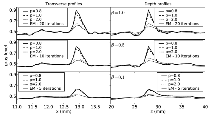
If, upon further study, it turns out that low $p$ image-reconstruction with ASD-POCS consistently yields improved contrast on microcalcification imaging, the implication for DBT imaging is enormous. It is known that microcalcification imaging is noise-limited, while mass imaging is structured-background limited. Image reconstruction algorithms that increase microcalcification detectability may lower the required intensity of the probing X-ray beam, thus lowering the radiation-dose of the DBT scan.

V.5 Case 2: uniform mass

Figure 9: ROI reconstructions of the data set containing a uniform mass by the EM algorithm at (left) 5, (middle) 10, and (right) 20 iterations. The gray scale window is [0.35,0.55].

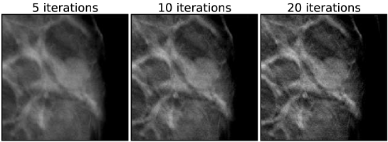
For the next case, there is a uniform mass, as can be seen in the EM image-reconstructions in Fig. 9. As was done in the previous case, we present a spread of images in Figs. 10, 11, and 12 from the ASD-POCS algorithm for the same sets of algorithm parameters, covering a range of $p$- and $\beta$-values. The iteration number dependence appears to be weak for ASD-POCS. The conspicuity of the mass for this case does not vary with algorithm parameters nearly as much as the microcalcification conspicuity of the previous case. There are many reasons for this. First, the X-ray attenuation coefficient of the mass is less than that of calcium, so the contrast that can be potentially regained is not as great. Second, the lower $p$ reconstructions tend to yield sharper edges, but this does not have as large an effect on the mass which is substantially bigger than microcalcifications. Finally, as pointed out earlier, mass conspicuity tends to depend on background structure noise. As this type of background is physically there, low $p$ image-reconstruction sharpens the edges of the background features just as much as the mass’s edges. Thus, the conspicuity of the mass may not improve dramatically as $p$ is lowered. In any case, there are subtle differences between the images, and these differences may have an impact on human or machine observers.

Figure 10: ROI reconstructions of the data set containing the uniform mass by the ASD-POCS framework with $\beta=1.0$. The gray scale window is held fixed, and is the same as that of the EM results, [0.35,0.55].

Figure 11: Same as Fig. 10 except $\beta=0.5$.

Figure 12: Same as Fig. 10 except $\beta=0.1$.

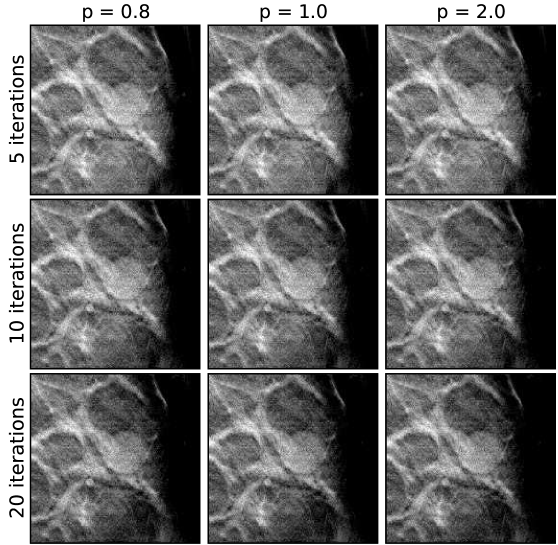
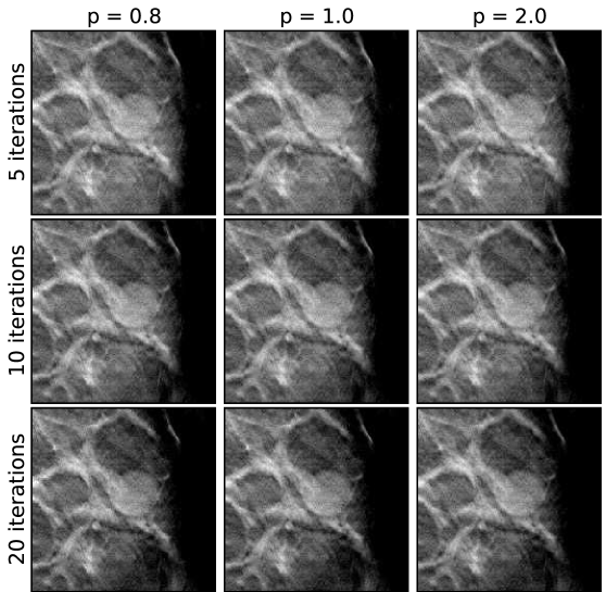
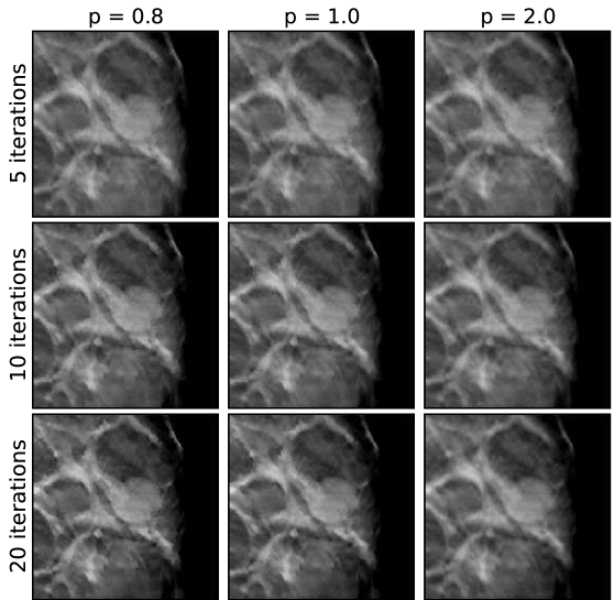
Comparing the visual quality of the images of the present case with the previous one, it is interesting that similar $\beta$-values do not yield similar apparent image quality. For example, $\beta=1.0$ for the present case appears to be quite noisy, even taking into account differing gray level windows, relative to $\beta=1.0$ for the previous case. For the 3 sets of $\beta$-values, $\beta=0.1$ appears to yield, visually, the best images for this mass case, while $\beta=0.5$ seems to best for the previous, microcalcification case. These, differences are likely due to varying quality of the acquired projection data. A quantitative discussion of algorithm performance across different DBT cases will be further elaborated on in Sec. V.7.

V.6 Case 3: spiculated mass in a dense breast

Figure 13: ROI reconstructions of the data set containing a spiculated mass in a dense breast by the EM algorithm at (left) 5, (middle) 10, and (right) 20 iterations. The gray scale window is [0.42,0.57].

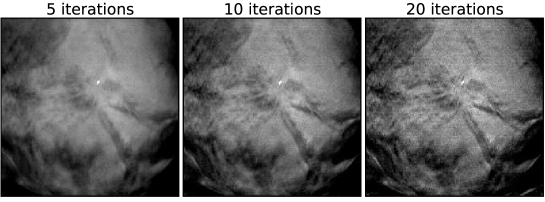
Finally, we present a case with a spiculated mass in dense breast tissue. It is precisely this type of case which DBT was developed for; by removing some of the interference of the overlapping structures such masses may be more conspicuous in DBT images than in standard mammographic projection imaging. The EM images are shown in Fig. 13, and the ASD-POCS images are shown in Figs. 14, 15, and 16. As with the previous mass case, there may be some advantage to image-reconstruction with ASD-POCS at low $p$ due to the fact that edges are enhanced. But the advantage is not as clear cut as it is with microcalcification imaging. Any advantage in mass imaging needs to be demonstrated by task-based image quality evaluation.

Figure 14: ROI reconstructions of the data set containing the spiculated mass in a dense breast by the ASD-POCS framework with $\beta=1.0$. The gray scale window is held fixed, and is the same as that of the EM results, [0.42,0.57].

Figure 15: Same as Fig. 14 except $\beta=0.5$.

Figure 16: Same as Fig. 14 except $\beta=0.1$.

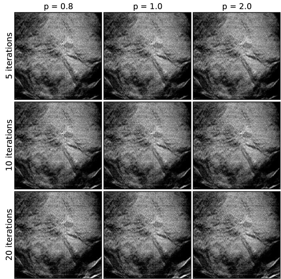
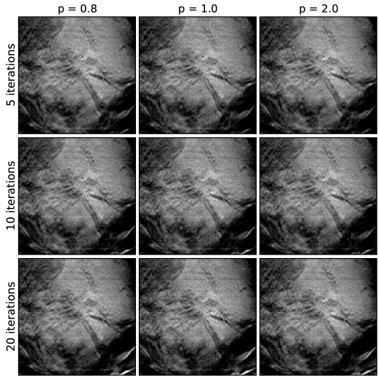
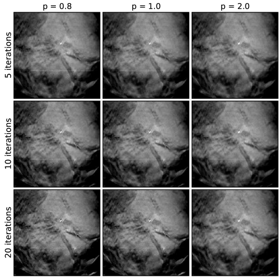
With this case, under-regularization, at large $\beta$, tends to yield linear artifacts in the image. Actually, similar lines appear for the other cases in the first two iterations of ASD-POCS, but the quickly disappear and are gone by the fifth iteration. These lines, for the present case, are likely due to a slight system misalignment or patient motion. This case reveals the control afforded by the $\beta$ parameter in the ASD-POCS algorithm. It is easy to select a value of $\beta$ small enough to wash out the linear artifacts without severely blurring the underlying features of the image.

V.7 Evolution of algorithm metrics

Figure 17: ASD-POCS versus EM parameter trajectories for the data sets containing (top) microcalcifications, (middle) a uniform mass, and (bottom) a spiculated mass. ASD-POCS with only $p=1.0$ is shown. In each case, the actual iteration numbers are indicated by the symbols starting at iteration 2, at the top of each curve, and increasing by 2 until 20 iterations at the bottom of the curves.

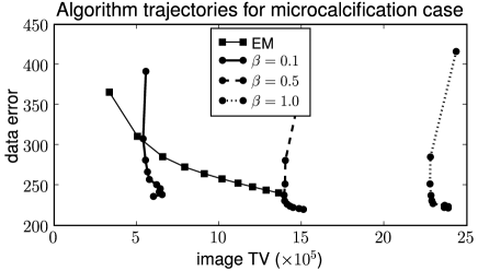
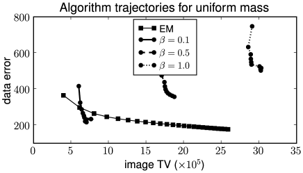
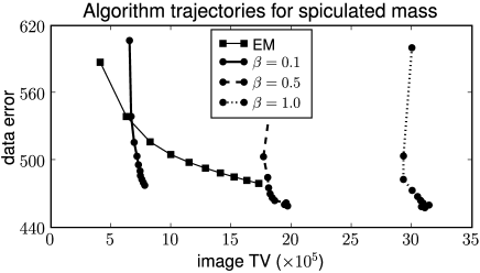
It is instructive to return to the discussion on the ASD-POCS algorithm, and examine the trajectories of the image estimates in the $R,\delta$-plane. Figure 17 shows this evolution for each of the three DBT cases for $p=1.0$. The plotted data error is given by:

$$\delta=\sqrt{(M\vec{f}-\tilde{g})\cdot(M\vec{f}-\tilde{g})},$$ (13)

and the objective function $R(\cdot)$ is Eq. (9) with $p=1.0$. It is primarily for the purpose of generating these graphs that the projection rays intersecting the compression paddle were excluded from the DBT projection data sets. Retaining these inconsistent rays would skew the values of the data error. Aside from differences in cropping the projection data, the algorithm parameters are the same for each of the three DBT data sets.

Recall that the goal in designing the current ASD-POCS algorithm is to be able to obtain images, within a few iterations (on the order of 10), corresponding to any point in as-much-as-possible of allowed region of the data error-TV plane. Starting with the microcalcification case, at the top of Fig. 17, the difference between the ASD-POCS and the standard EM algorithm is clear. Reducing the value of $\beta$ seems to directly reduce image TV, and the adaptive component of the ASD-POCS allows the data error to be reduced with little change in image TV. The last iteration shown, number 20, at the bottom of each of the three $\beta$ curves, is the minimum data-error image in the sequence. Interestingly, this minimum data-error value seems to have little dependence on $\beta$ even though the image TV is dramatically reduced by lowering $\beta$. This is not surprising due to the fact that the DBT system is very much undersampled in the angular direction; many images with very different TV-values may correspond to the same data-error. The track of the EM algorithm shows the traditional trade-off for most iterative algorithms. As iteration number is increased data-error is reduced at the expense of image regularity. For this particular EM run, no TV regularization was used. But incorporating such regularization in EM, for example by the method discussed in Refs. Lange (1990); Persson et al. (2001), results in an iteration track of similar shape. It is still difficult to obtain images for the low-data-error, low-TV corner with a non-adaptive iterative algorithm. We point out that the ASD-POCS algorithm likely cannot explore the complete allowed region of the data error-TV plane, especially within a few iterations. And there is room for further algorithm development in pushing toward low-data-error and low-image-TV.

Turning to the DBT case with the uniform mass, shown in the middle graph in Fig. 17, the algorithm trajectories are similar to the previous case aside from one aspect. There is a significant drop in data error obtained by reducing $\beta$ from 1.0 to 0.1 . This trend is counter-intuitive, because greater image regularity is generally obtained at the expense of data fidelity. In this case, imposing greater image regularity allows for greater progress in reducing data-error. This type of behavior, we have observed before in image-reconstruction from simulated data; it generally occurs when the primary component of the data error is noise in the detector bin measurements. The data for this case is noisier than that of the previous, microcalcification case. This is seen in the reconstructed images, and the raw projection data show higher X-ray attenuation. Yet, the minimum data-error reached, at $\beta=0.1$, is comparable to minimum values reached for the microcalcification case.

Examining the curves for the spiculated-mass case, the shape of the curves is similar to that of the microcalcification case. The difference between this case and the previous two is the value of the minimum data-error achieved. It is roughly a factor of two higher than the previous cases. Again, as this is a dense breast, the data noise is relatively high. But as $\beta$ is decreased the data error remains high. We speculate that the reason for this is that there may be additional error due to incorrect geometry, such as patient motion during the scan.

Studying the algorithm trajectories in the data-error, image-regularity plane helps to understand the image-reconstruction algorithm. Such curves may also prove useful in determining data quality. Clearly, for ideal data, a data-error of zero can be reached. Data-error values, however, will in general be finite, but it may be also important to know the source of the data inconsistency. If these curves can be used to reveal data-error due to patient motion, they have additional, practical value. For example, imaging microcalcifications is highly dependent on the absence of motion. If a particular scan reveals no microcalcifications and the algorithm trajectories suggest patient motion is likely present, it may be advisable to do a re-scan.

VI discussion

We have introduced a practical, iterative image-reconstruction algorithm, within the ASD-POCS framework, that can achieve useful images within a few iterations. This algorithm allows for fine control over the regularity of the reconstructed images, which is essential for under-determined imaging problems such as DBT. For the studies presented here, the image regularity metric is taken to be the total $p$-variation, which reduces to the total variation and the image roughness for $p=1.0$ and $p=2.0$, respectively. The other main algorithm parameter, $\beta$, controls the level of the regularity objective-function. As with all other iterative algorithms, the iteration number is implicitly another parameter. The main advantage of the present algorithm is that each of these few parameters have a real effect on the image quality, and these effects are relatively independent of each other.

For DBT imaging, microcalcification imaging is the task that appears to be most greatly impacted by the present algorithm. Images reconstructed with low values of $p$ show markedly greater contrast of the microcalcifications than those reconstructed by existing algorithms. The practical significance of this increased contrast is that it may be possible to reduce the X-ray intensity thereby lowering patient dose for the DBT scan. The effects for mass imaging are more subtle, but the finer controls allowed by the present algorithm may allow better optimization of the DBT system for mass imaging by either human or computer observers.

Extensions of this work can follow many different paths. Within the ASD-POCS framework, various methods of performing the adaptive control may lead to more efficient image-reconstruction algorithms. Also different objective functions, which can simply be dropped into the present framework, may be advantageous for different imaging tasks. One practical question that we intend to investigate is to use the ASD-POCS framework together with algorithm trajectories to provide an assessment of projection data quality, particularly, to find a way to automatically detect patient motion.

We point out that the algorithm presented here, though applied to DBT imaging, can easily be adapted to other X-ray based tomographic systems. In fact, other tomographic imaging modalities with a linear data model may also be amenable to image-reconstruction within the ASD-POCS framework.