Gravity-driven instabilities: interplay between state-and-velocity dependent
frictional sliding and stress corrosion damage cracking

Abstract.

We model the progressive maturation of a heterogeneous mass towards a gravity-driven instability, characterized by the competition between frictional sliding and tension cracking, using array of slider blocks on an inclined basal surface, which interact via elastic-brittle springs. A realistic state- and rate-dependent friction law describes the block-surface interaction. The inner material damage occurs via stress corrosion. Three regimes, controlling the mass instability and its precursory behavior, are classified as a function of the ratio $T_{c}/T_{f}$ of two characteristic time scales associated with internal damage/creep and with frictional sliding. For $T_{c}/T_{f}\gg 1$, the whole mass undergoes a series of internal stick and slip events, associated with an initial slow average downward motion of the whole mass, and progressively accelerates until a global coherent runaway is observed. For $T_{c}/T_{f}\ll 1$, creep/damage occurs sufficiently fast compared with nucleation of sliding, causing bonds to break, and the bottom part of the mass undergoes a fragmentation process with the creation of a heterogeneous population of sliding blocks. For the intermediate regime $T_{c}/T_{f}\sim 1$, a macroscopic crack nucleates and propagates along the location of the largest curvature associated with the change of slope from the stable frictional state in the upper part to the unstable frictional sliding state in the lower part. The other important parameter is the Young modulus $Y$ which controls the correlation length of displacements in the system.

1. Introduction

Gravity-driven instabilities include landslides, mountain collapses, rockfalls, ice mass break-off and snow avalanches. They pose a considerable risk to mountain communities, real-estate development, tourist activities and hydropower energy generation. Gravity-driven instabilities are the most widespread natural hazard on Earth. Most of these consist of slumping masses of soil, too small to be lethal but costly in term of property damage, especially when they are close to roads, railway lines and built-up areas. At the other extreme is the infrequent occurrence of the collapse of a mountainside which can release the energy equivalent of a major volcanic eruption or earthquake within seconds. Such collapses are among the most powerful hazards in nature and can wreak devastation over tens of square kilometers. In the US and Europe in particular, gravity-driven instabilities at all scales are particularly significant and cause billions of dollars and euros in damage each year.

Gravity-driven instabilities occur in a wide variety of geomechanical contexts, geological and structural settings, and as a response to various loading and triggering processes. They are often associated with other major natural disasters such as earthquakes, floods and volcanic eruptions. Some slope instabilities involve the rupture and collapse of entire mountains, with devastating consequences. One of the most spectacular rockslides that ever occurred in the world is the Köfels rockslide [Erismann and Abele, 2001], in which more than $3\;\rm km^{3}$ of rock was released in a short time span. This event occurred approximately 9,600 years ago. Many other large and giant historic and prehistoric rockslides have been described by Heim [1932], Abele [1974] and Erismann and Abele [2001]. Recent spectacular landslides in the European Alps include the Vaiont disaster, which resulted in about 2,000 casualties when a $0.3\;\rm km^{3}$ sliding mass fell into a hydro-electric power reservoir in 1963 [Müller, 1964]. Another example is the Val Pola slide, damming up the valley in 1987 [Azzoni et al., 1992]. Much can also be learned from frequent and historically reported giant and rapid landslides on the slopes of many volcanoes [Moore et al., 1994; McMurtry et al., 1999; Clouard et al., 2001]. These are often associated with either caldera collapse [Hurlimann et al., 2000] or volcanic eruption [Voight, 1988; Heinrich et al, 1999]. Earthquakes are other triggering processes, which have to be considered.

The present paper develops a model of the progressive maturation of a mass towards a gravity-driven instability, which combines basal sliding and cracking. Our hypothesis is that gravity-driven ruptures in natural heterogeneous material are characterized by a common triggering mechanism resulting from a competition between frictional sliding and tension cracking. Heterogeneity of material properties and dynamical interaction seem to have a significant influence on the global behavior. Our main goal is thus to understand the role of the competition or interplay between the two physical processes of sliding and tension cracking in the early stages of an instability. The run-up to the sliding instabilities can be described by applying a modern constitutive law of state-and-velocity dependent friction. This means that solid friction is not used as a parameter but as a process evolving with the concentration of deformation and properties of sliding interfaces. Cracking and fragmentation in the mass is accounted for by using realistic laws for the progressive damage accumulation via stress corrosion and other thermally activated processes aided by stress. In one sense, the present paper can be considered as an important extension of [Helmstetter et al., 2004; Sornette et al., 2004], who modeled the potentially unstable mass by means of a single rigid slider block interacting with a inclined basal surface via solid friction. These authors showed that the use of a realistic state- and rate-dependent friction law established in the laboratory could provide a reasonable starting point for describing the empirical displacement and velocity data preceding landslides. Here, we use an array of such slider blocks on an inclined (and curved) basal surface, which interact via elastic-brittle springs. The springs, which model the inner material properties of the mass, also undergo damage, eventually leading to failure. By combining both sliding and damage processes in a single coherent model, this paper contributes to the literature by providing

• a better understanding of the relative role of and interplay between the frictional and rupture processes,

• a quantification of the transition from slow stable landsliding to unstable and fast catastrophes events,

• a theory of potential precursors to catastrophic slope failure,

• a model to exploit the increasing availability of continuous monitoring by geodetic, GPS, SAR measurements as well as geophysical measurements to obtain advanced warnings,

• a framework to assess the impact of varying climatic conditions and/or external forcing (rain, snow, passing seismic waves, etc.), and

• a framework for developing strategies to mitigate the hazard resulting from gravity-driven instabilities.

In Section 2, we provide a summary of previous works related to gravity-driven instabilities, and focus particularly on the different strategies employed to investigate stability. Section 3 is devoted to a detailed description of the proposed model. Section 4 presents an application of this numerical model to a hanging glacier and a comparison between numerical and experimental results. Conclusions are presented in Section 5.

2. Summary of previous related works

At the longest time scales, gravity-driven instabilities have been studied historically by the method of slope stability analysis developed in civil engineering, which was developed to ensure the safety of man-made structures, such as dams and bridges. This method usually divides a profile view of the mass of interest into a series of slices, and calculates the average factor of safety for each of these slices, using a limit equilibrium method [e.g. Hoek and Bray, 1981; Blake et al., 2002]. The factor of safety is defined as the ratio of the maximum retaining force to the driving forces. Geomechanical data and properties are inserted in finite elements or discrete elements of numerical codes, which are run to predict the possible departure from static equilibrium or the distance to a failure threshold. This is the basis of landslide hazard maps, using safety factors greater than $1$. In this modeling strategy, the focus is on the recognition of time-independent landslide-prone areas. Such an approach is similar to the practice in seismology called “time-independent hazard,” where earthquake-prone areas are located relative to active faults, for instance, while the prediction of a single, individual earthquake is recognized to be much more difficult, if not unattainable. This “time-independent hazard” essentially amounts to assuming that gravity-driven instabilities result from a random (Poisson) process in time, and uses geomechanical modeling to constrain the future long-term hazard. In this model, failure appears to occur without warning, probably because earlier movements have passed unnoticed. The approaches in terms of a factor of safety do not address the possible preparatory stages leading to the catastrophic collapse.

In contrast, “time-dependent hazard” would accept a degree of predictability in the process, because the hazard associated with the potential triggering of gravity-driven instabilities varies with time, perhaps in association with varying external factors (rain, snow, volcanic). For instance, accelerated motions have been linked to pore pressure changes [e.g. Vangenuchten and Derijke, 1989; Van Asch et al., 1999], leading to an instability when the gravitational pull on a slope exceeds the resistance at a particular subsurface level. Since pore pressure acts at the level of submicroscopic to macroscopic discontinuities, which themselves control the global friction coefficient, circulating water can hasten chemical alteration of the interface roughness, and pore pressure itself can force adjacent surfaces apart. Both effects can produce a reduction in the friction coefficient which leads, when constant loading applies, to accelerating movements [Kuhn and Mitchell, 1993]. However, this explanation has not lead to a quantitative method for forecasting slope movement.

The next level in the hierarchy of models would be “gravity-driven instability forecasting,” which would require significantly better understanding to enable the prediction of some of the features of an impending catastrophe, usually on the basis of the observation of precursory signals. Practical difficulties include identifying and measuring reliable, unambiguous precursors, and the acceptance of an inherent proportion of missed events or false alarms. Let us also mention the approach developed by [Iverson, 1985; 1986a; 1986b; 1993; Iverson and Reid, 1992] based on coupled pressure-dependent plastic yield and nonlinear viscous flow deformations (see also [Iverson and Reid, 1992]). According to the theory of Iverson et al., the plastic yield is a generalization of the Coulomb criterion to three-dimensional stress states in the spirit of Rice [1975], and the effect of pore-water pressures is accounted for by the use of the Terzaghi “effective” stresses. This theory embodies as special cases models of creeping, slumping, sliding and flowing types of slope deformation. The underlying equations remain fundamentally based on continuum mechanics, which differentiates it from our approach which focuses on the dominating role of sliding interfaces/bands and their rheology controlled by discrete asperities, joints and blocks.

There exists a common phenomenology prior to rupture, which is observed in many different natural materials and geophysical set-ups. In particular, there are well-documented cases of precursory signals, showing accelerating slip-over time scales of weeks to decades. We mentioned before the Vaiont landslide on the Mt Toc slope in the Dolomite region in the Italian Alps, which was the catastrophic culmination of an accelerated slope velocity (see for instance [Helmstetter et al., 2004; Sornette et al., 2004] for the data and a recent analysis in terms of accelerated precursory sliding velocity). More precisely, gravity-driven instabilities often exhibit a finite time singularity characterized by a power law behavior of some variable (such as displacement or deformation, velocity of the instable mass or acoustic emissions) as a function of time. This behavior is quite common in a wide class of nonlinear process, including gravity-driven instability such as rockfall [Amitrano et al., 2005], landslides [Helmstetter et al., 2004; Sornette et al., 2004], break-off of ice chunks from hanging glaciers [Flotron, 1977; Röthlisberger, 1981; Lüthi, 2003; Pralong and Funk, 2005, Pralong et al., 2005], but also for earthquakes [Bufe and Varnes, 1993; Bowman et al., 1998; Jaumé and Sykes, 1999; Sammis and Sornette, 2002], and volcanic eruption [Voight, 1988]. Analogous behaviors have also been associated with financial crashes, with the dynamics of the economy and of population [Johansen and Sornette, 2001; Ide and Sornette 2002]. In other cases which exhibited accelerated deformations , such as La Clapière mountain [Helmstetter et al., 2004] in the southern Alps near St-Etienne-de-Tinée, France, the sliding can undergo a transition towards a slower more stable regime. While only a few such cases have been monitored in the past, modern monitoring techniques are bound to provide a wealth of new quantitative observations based on GPS and SAR (synthetic aperture radar) technology to map the surface velocity field [Mantovani et al., 1996; Parise, 2001; Fruneau et al., 1996; Malet et al., 2002; Berardino et al., 2003; Coe et al., 2003; Colesanti et al., 2003; Mora et al., 2003; Wasowski and Singhroy, 2003] and seismic monitoring of slide quake activity [Gomberg et al., 1995; Xu et al., 1996; Rousseau, 1999; Caplan-Auerbach et al., 2001].

Other studies proposed that rates of gravity-driven mass movements are controlled by microscopic slow cracking and, when a major failure plane is developed, the abrupt decrease in shear resistance may provide a sufficiently large force imbalance to trigger a catastrophic slope rupture [Kilburn and Petley, 2003]. Such a mechanism, with a proper law of input of new cracks, may reproduce the acceleration preceding of the collapse that occurred at Vaiont, Mt Toc, Italy [Kilburn and Petley, 2003].

An alternative modeling strategy consists in viewing the accelerating displacement of the slope prior to the collapse as the final stage of the tertiary creep preceding failure [Saito and Uezawa, 1961; Saito, 1965; 1969; Voight and Kennedy, 1979; Voight, 1988; 1989; 1990; Fukuzono, 2000; Kuhn and Mitchell, 1993]. Further progress in exploring the relevance of this mechanism requires a reasonable knowledge of the geology of the sliding surfaces, their stress-strain history, the mode of failure and the time-dependent shear strength along the surface of failure [Bhandari, 1988]. Unfortunately, this range of information is not usually available. This mechanism is therefore used mainly as a justification for the establishment of empirical criteria of impending landslide instability.

Observations of landslides have been quantified by what amounts to a scaling law relating the slip acceleration $d\dot{\delta}/dt$ to the slip velocity $\dot{\delta}$ according to the following equation [Voight, 1990; Voight and Kennedy, 1979; Petley et al., 2002]

(2.1) $$d\dot{\delta}/dt=A\dot{\delta}^{\alpha}~{},$$

where $A$ and $\alpha$ are empirical constants. For $\alpha>1$, this relationship predicts a divergence of the sliding velocity in finite time at some critical time $t_{f}$, which is determined by the parameters $A$ and $\alpha$ and the initial value of the velocity. The mathematical divergence is of course not to be taken literally: it signals a bifurcation from accelerated creep to complete slope instability for which inertia is no longer negligible and other processes such as liquefaction (not necessarily involving fluids) come into play. Several cases have been quantified ex-post with this law, usually using $\alpha=2$, by plotting the time $t_{f}-t$ to failure as a function of the inverse of the creep velocity [Bhandari, 1988]. In fact, the solution of (2.1) for $\alpha>1$ can be expressed as

(2.2) $$t_{f}-t\sim 1/\dot{\delta}^{1\over\alpha-1}~{}.$$

These fits suggest that it might be possible to forecast impending landslides by recording accelerated precursory slope displacements. As a matter of fact, for Mont Toc, Italy, Vajont landslide, Voight [1988] mentioned that a prediction of the failure date could have been made more than 10 days before the actual failure by using (2.2) with $\alpha=2$. The physically based friction model [Helmstetter et al., 2004; Sornette et al., 2004] which avoids such a priori assumption has confirmed this claim.

Figure 1. Simplified synopsis of the range of time scales, the associated sliding velocities and the major processes involved in the evolution of slopes (see for example [Brunsden, 1999] for a review). Our model is applied to the intermediate range from years to tens of minutes before the catastrophic collapse, as indicated in boldface. This graph was prepared with the help of G. Ouillon.

Voight [1988; 1989] proposed that relation (2.1), which generalizes damage mechanics laws [Rabotnov, 1980; Gluzman and Sornette, 2001], can be used with other variables (including strain and/or seismic energy release) for a large variety of materials and loading conditions [Sammis and Sornette, 2002]. Equation (2.1) seems to apply as well to diverse types of landslides occurring in rock, soil and ice, including first-time and reactivated slides [Voight, 1988]. It may be seen as a special case of a general expression for failure [Voight, 1988; 1989; Voight and Cornelius, 1991]. Recently, such time-to-failure laws have been interpreted as resulting from cooperative critical phenomena and have been applied to the prediction of failure of heterogeneous composite materials [Anifrani et al., 1995] and to precursory increase of seismic activity prior to main shocks [Sornette and Sammis, 1995; Jaume and Sykes, 1999; Sammis and Sornette, 2002]. See also [Sornette, 2002] for extensions to other fields.

The law (2.1) may apply over time scales from years to tens of minutes before the run-out, as summarized in Figure 1. Our model provides a general conceptual and operational framework to rationalize the law (2.1). One of the strengths of our approach is to be able to tackle in the same conceptual framework both stable slope evolutions as well as unstable regimes culminating in a runout. Our approach applies to any landslides, irrespective of their final catastrophic evolution in the runout regime, because we focus on the quasi-static regime in which the slope can still be analyzed as a system of interacting sliding blocks. While we model the progressive damage and rupture between sliding blocks, we do not describe the final stage of the dynamic runout during which most large landslide disintegrate in rapid motion in a collection of blocks as they move down the slope (as an example of this, see [Campbell 1989; 1990; Cleary and Campbell, 1993; Campbell et al., 1995]). This final dynamic regime includes additional physical mechanisms that we do not account for: (i) heat-generated pore pressure inside a rapidly deforming shear band [Voight and Faust, 1982a,b], (ii) thermo-poro-mechanical softening of the soil [Vardoulakis, 2002a,b] and (ii) shear-induced pore dilation which leads to unstability when sediments are dilated to their critical-state porosity (see for instance [Moore and Iverson, 2002]). These models predict exponential accelerations only in the last tens of seconds when the sliding velocity is sufficiently large. Finally, the runout itself is characterized by further mechanisms associated with velocities reaching such large values (meter/s to tens of meters/s) that inertial effects are no longer negligible (see Figure 1). These two times scales are not addressed in our approach, which focuses on the stability and possible destabilizations of slopes over time scales from years to tens of minutes.

3. Geometry and physical inputs of the model

3.1. Main elements of the model

To tackle the challenge of modeling the interplay between the two physical processes of sliding and tension cracking in the preparatory stages of a gravity-driven instability, we proposed a discrete set-up made of block masses linked to each other by elastic springs. The blocks slid on a basal inclined surface and interacted via direct elastic coupling to the neighboring blocks.

A toy model embodying the principles of competition between subsurface slip and the possible growth of cracks decoupling adjacent blocks was developed by Andersen et al. [1997] and Leung and Andersen [1997]. Many other investigators have studied spring-block models, but most were derived from the Burridge-Knopoff prototype having elastic coupling with an upper rigid plate, as a simple representation of the tectonic driving which lead to earthquakes. Note that such elastic coupling to an upper plane entails the wrong large scale elastic limit for gravity-driven masses. In contrast, the blocks in the Andersen et al. [1997]’s model are only connected to nearest neighbors and are in frictional contact with a substrate. Meakin and collaborators [Meakin, 1991] have also studied a similar model in the context of drying patterns.

Using blocks as representative discrete interacting elements provides a reasonable starting point for describing the processes occurring before the complete destabilization of the slope. Actually, a model with just one block was used by [Heim, 1932; Korner, 1976; Eisbacher, 1979; Davis et al., 1990]. In these works, the friction coefficient between the rigid block and surface is usually imposed as a constant, or just either slip- or velocity-dependent (but not slip- and velocity-dependent). A constant solid friction coefficient (Mohr-Coulomb law) is often taken to simulate mass over bedrock sliding. A slip-dependent friction coefficient model is taken to simulate the yield-plastic behavior of a brittle material beyond the maximum of its strain-stress characteristics. For rock avalanches, Eisbacher [1979] suggested that the evolution from a static to a dynamic friction coefficient is induced by the emergence of a basal gauge. Studies using a velocity-dependent friction coefficient have focused mostly on the establishment of empirical relationships between shear stress $\tau$ and block velocity $v$, such as $v\sim\exp[a\tau]$ [Davis et al., 1990] or $v\sim\tau^{1/2}$ [Korner, 1976], however without a definite understanding of the possible mechanism. Muller and Martel [2000] also point out that near the surface, principal stresses are either normal or parallel to the local slope; thus shear stress on planes parallel to the slope must be small. This implies that slip must initiate on pre-existing planes of weakness.

Our present model improves on these models and on the multi-block model of Andersen et al. [1997] and Leung and Andersen [1997] in two ways. First, we use a state-and-velocity weakening friction law instead of a constant (or just state- or velocity-weakening) solid friction coefficient. Second, rather than a static threshold for the spring failures, we model the progressive damage accumulation via stress corrosion and other thermally activated processes aided by stress. Both improvements make the numerical simulations significantly more involved but present the advantage of embodying rather well the known empirical phenomenology of sliding and damage processes. Adding the state and velocity-dependent friction law and time-dependent damage processes allows us to model rather faithfully the interplay between sliding, cracking between blocks and the overall self-organizing of the system of blocks. This will allow us to investigate the following questions: what are the conditions under which cracking (disconnection between blocks) can stabilize sliding? What is the effect of heterogeneity along the slope? Can we construct a simple set of blocks and their interactions that can reproduce the complex history of some slopes, such as the case studies presented in Section 4.

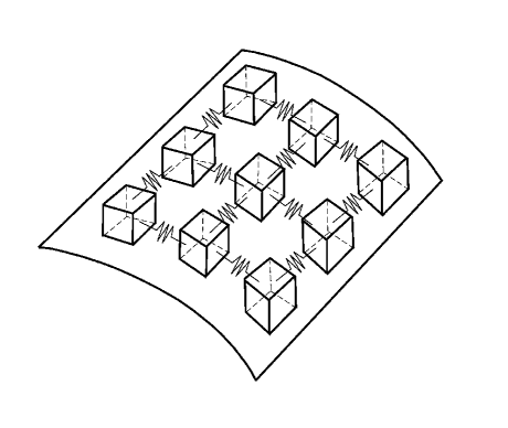
The geometry of the system of blocks interacting via springs and with a basal surface is depicted in Figure 2. The model includes the following characteristics:

1. frictional sliding on the ground or between layers,

2. heterogeneity of basal properties,

3. possible tension rupture by accumulation of damage,

4. dynamical interactions of damage or cracks along the sliding layer,

5. geometry and boundary conditions,

6. interplay between frictional sliding and cracking.

We now turn to the specification of the two key ingredients, the friction and damage laws, that are applied to blocks and bonds respectively.

Figure 2. Illustration of the model constisting of spring-blocks resting on an inclined slope. The blocks lie on an inclined curved surface and gravity is the driving force. Only a small subset of the spring-block system is shown here.

3.2. Friction law between the discrete blocks and the basal surface

3.2.1. State- and rate-dependent solid friction

State- and velocity-dependent friction laws have been established on the basis of numerous laboratory experiments (see, for instance, [Scholz, 2002; 1998; Marone, 1998; Gomberg et al., 2000] for reviews). Friction laws have been investigated in the laboratory using mainly strain-controlled tests in which, for instance, motion of a slider block is driven by controlling its velocity. This strain-controlled set-up is thought to be relevant to faults which are generally assumed to be driven by far-field forces transmitted via elastic and inelastic deformations. In contrast, gravity-driven masses move chiefly in response to changes in the mix of internal body forces imposed by gravity and pore-pressure fields. In this context, stress-controlled experiments are more relevant. Dieterich [1994] has shown that his strain-controlled friction law does apply to stress-controlled interactions between ruptures. Many other works have used these friction law in stress-controlled situations (see e.g. [Lapusta et al., 2000; Ben-Zion and Rice, 1997]). Experiments have also confirmed that the state- and velocity-dependent friction laws established with strain-controlled experiment apply equally well (with a slight modification with regularization) to stress-controlled situations [Prakash and Clifton, 1993; Prakash, 1998; Ben-Zion, 2001; Berger, 2002].

Analogies between landslide faults and tectonic faults [Gomberg et al., 1995] and the relevance of a solid friction criterion for pre-existing slopes with weak layers or geologic discontinuities, with bedding planes, landslide slip-surfaces, faults, or joints, or for existing landslides, suggest that the improved description of the friction coefficient that we use here be viewed as an a element essential to the understanding of slope evolutions. To our knowledge, Helmstetter et al. [2004] and Sornette et al. [2004] were the first to explore quantitatively the analogy between sliding rupture and earthquakes and to use the physics of state- and velocity-dependent friction to model gravity-driven instabilities and their precursory phases (see [Brabb, 1991; Cruden, 1997; Guzetti et al., 1999; Howell et al., 1999; Al-Homoud and Tahtamoni, 2001] for a compilation of cases). Earlier, Chau [1995, 1999] also used the state- and rate-dependent friction law (3.1) given below to model gravity-driven instabilities. He transformed the problem into a formal nonlinear stability analysis of the type found in mathematical theory of dynamical systems, but no physical application was described. In particular, Chau’s analysis missed the existence of the finite-time singular behavior found also empirically, as discussed above and recalled below.

The key concept underlying the state- and rate-dependent friction law is that the friction coefficient $\mu$ between a block and the inclined basal surface supporting it evolves continuously as a function of cumulative slip $\delta$, slip velocity $\dot{\delta}$ and time, as shown by experiments carried over a large range of time scales, under static or sliding conditions over a large range of velocities, for a wealth of different materials. The version of the rate/state-variable constitutive law, currently most accepted as being in reasonable agreement with experimental data on solid friction, is known as the Dieterich-Ruina law [Dietrich, 1994]:

(3.1) $$\mu(\dot{\delta},\theta)=\mu_{0}+A\ln{\dot{\delta}\over\dot{\delta}_{0}}+B\ln{\theta\over\theta_{0}}~{},$$

where the state variable $\theta$ is usually interpreted as the proportional to the surface of contact between asperities of the two surfaces. The constant $\mu_{0}$ is the friction coefficient for a sliding velocity $\dot{\delta}_{0}$ and a state variable $\theta_{0}$. $A$ and $B$ are coefficients depending on material properties. Expression (3.1) as written is not appropriate for very low or vanishing values of sliding velocities and a simple regularization near $\dot{\delta}=0$ can be performed, that is motivated by Arrhenius thermal activation of creep at asperity contacts [Ben-Zion, 2003]. The time evolution of the state variable $\theta$ is described by

(3.2) $${{\rm d}\theta\over{\rm d}t}=1-{\theta\dot{\delta}\over D_{c}}~{},$$

where $D_{c}$ is a characteristic slip distance, usually interpreted as the typical size of asperities. We note that (3.2) can be rewritten

(3.3) $${{\rm d}\theta\over{\rm d}\delta}={1\over\dot{\delta}}-{\theta\over D_{c}}~{}.$$

For small or zero sliding velocity, $\theta$ grows linearly with time. Using the above-mentioned regularization [Ben-Zion, 2003], this gives a logarithmic strengthening of $\mu$. For a steady-state non-zero velocity, we have [Scholz, 1998] $\mu={\hat{\mu}}_{0}+(A-B)\ln[\dot{\delta}/\dot{\delta}_{0}]$, where ${\hat{\mu}}_{0}=\mu_{0}+B\ln{D_{c}\over\theta_{0}\dot{\delta}_{0}}$. Thus, the derivative of the steady-state friction coefficient with respect to the logarithm of the reduced slip velocity is $A-B$. If $A>B$, this derivative is positive: friction increases with slip velocity and the system is stable as more resistance occurs which tends to react against the increasing velocity. In contrast, for $A<B$, friction exhibits the phenomenon of velocity-weakening and is unstable.

The primary parameter that determines stability, $A-B$, is a material property. For instance, for granite, $A-B$ is negative at low temperatures (unstable) and becomes positive (stable) for temperatures above about 300^∘C. In general, for low-porosity crystalline rocks, the transition from negative to positive $A-B$ corresponds to a change from elastic-brittle deformation to crystal plasticity in the micro-mechanics of friction [Scholz, 1998]. For the application to gravity-driven instabilities, we should in addition consider that sliding surfaces are not only contacts of bare rock surfaces: they are usually lined with wear detritus, called cataclasite or gouge in the case of faults or joints. The shearing of such granular material involves an additional hardening mechanism (involving dilatancy), which tends to make $A-B$ more positive. For such materials, $A-B$ is positive when the material is poorly consolidated, but decreases at elevated pressure and temperature as the material becomes lithified. See also Section 2.4 of Scholz’s book [Scholz, 2002] and the discussion below. The friction law (3.1) with (3.2) accounts for the fundamental properties of a broad range of surfaces in contact, namely that they strengthen (age) logarithmically when aging at rest, and tend to weaken (rejuvenate) when sliding.

3.2.2. Frictional dynamics

Let us first consider a single block and the base in which it is encased. The block represents the discrete element of the slope which may be potentially unstable. The two main parameters controlling the stability of the block are the angle $\phi$ between the surface on which the block stands and the horizontal and the solid friction coefficient $\mu$. The block exerts stresses that are normal ($\sigma$) as well as tangential ($\tau$) to this surface of contact. The angle $\phi$ controls the ratio of the shear over normal stress: $\tan\phi=\tau/\sigma$. In a first step, we assume for simplicity that the usual solid friction law $\tau=\mu\sigma$ holds for all times. Four possible regimes are found, that depend on the ratio $B/A$ of two parameters $A$ and $B$ of the rate and state friction law and on the initial frictional state of the sliding surfaces characterized by a reduced parameter

(3.4) $$X_{i}=(S\;\theta_{0})^{1/(1-B/A)}~{}{\theta\over\theta_{0}}~{},~{}~{}~{}~{}~{}\;\;\;{\rm for}~{}A\neq B~{},$$

where

(3.5) $$S\equiv{\dot{\delta}_{0}\over D_{c}}~{}e^{{\tau\over\sigma}-\mu_{0}\over A}$$

depends on the material properties but not on the initial conditions, and $\theta_{0}$ represents the initial value of the state variable.

Helmstetter et al. [2004] have shown that two regimes among them can account for an acceleration of the displacement. For $B/A>1$ (velocity weakening) and $X_{i}<1$, the slider block exhibits an unstable acceleration leading to a finite-time singularity of the displacement and of the velocity $v\sim 1/(t_{f}-t)$, thus rationalizing Voight’s empirical law discussed in Section 2. An acceleration of the displacement can also be reproduced in the velocity strengthening regime, for $B/A<1$ and $X_{i}>1$. In this case, the acceleration of the displacement evolves toward a stable sliding with a constant sliding velocity. The two others cases ($B/A<1$ and $X_{i}<1$, and $B/A>1$ and $X_{i}>1$) give a deceleration of the displacement.

The case $B=A$ is of special interest because it retrieves the main qualitative features of the two classes, and also because, empirically, $A$ is very close to $B$. It may be natural to assume that $A=B$ to remove the need for one parameter and ensure more robust results. In the sequel, we use this approximation $A\approx B$. In this case, expression (3.2) renders

(3.6) $${{\rm d}\theta\over{\rm d}t}=1-S\;\theta_{0}~{}.$$

If $S\;~{}\theta_{0}>1$ and is a constant, $\theta$ decays linearly and reaches $0$ in finite time. This retrieves the finite-time singularity, with the slip velocity diverging as $1/(t_{f}-t)$ corresponding to a logarithmic singularity of the cumulative slip. If $S\;~{}\theta_{0}<1$ and is a constant, $\theta$ increases linearly with time. As a consequence, the slip velocity decays as $\dot{\delta}\sim 1/t$ at large times and the cumulative slip grows asymptotically logarithmically as $\ln t$. This corresponds to a standard plastic hardening behavior.

Appendix A calculates the critical time $t_{f}$ (for $S\theta_{0}>1$) as a function of the total shear force $T\equiv\Arrowvert\sum\vec{F}_{\rm bond}\;-\;T_{\rm weight}\vec{x}\Arrowvert$ and the normal force $N\equiv N_{\rm weight}$ exerted on a given block, where $\vec{F}_{\rm bond}$ is the force exerted by a neighboring spring bond, $N_{\rm weight}$ and $T_{\rm weight}$ are the normal and tangential forces due to the weight of the block. These forces enter into the value of $S$ defined by (3.5) via $\tau$ and $\sigma$. From the definition of a solid friction coefficient ($\mu=\frac{T}{N}$), the critical time $t_{f}$ signaling the transition from a subcritical sliding to the dynamical inertial sliding is, for $\mu>\mu_{0}$,

(3.7) $$t_{f}\;=\;\frac{\theta_{0}}{\exp(\frac{\mu-\mu_{0}}{A})-1}~{},$$

while $t_{f}\to\infty$ for $\mu\leq\mu_{0}$.

3.2.3. General algorithm of the frictional processes

The simulation of the frictional process for each given block proceeds as follows:

1. A given configuration of blocks and spring tensions determines the value of $T\equiv\Arrowvert\sum\vec{F}_{\rm bond}\;-\;T_{\rm weight}\vec{x}\Arrowvert$ and $N\equiv N_{\rm weight}$ for each block, and therefore of their solid friction coefficient $\mu$ equal to the ratio $T/N$.

2. Knowing $\mu$ for a given block and with the other material parameters $\theta_{0},\mu_{0}$ and $A$ for that block, the time $t_{f}$ for the transition to the dynamical sliding regime for that block is calculated with expression (3.7). The formula (3.7) for $t_{f}$ gives, therefore, the waiting time until the next slide of that block.

3. When the block undergoes a transition into the dynamical sliding regime at time $t_{f}$, its subsequent dynamics is taken to obey Newton’s law.

4. Following other investigators [Farkas et al., 2005; Persson, 1993], we assume that, when the dynamical sliding phase starts, the friction coefficient decreases abruptly from its value attained at time $t_{f}$ to a smaller dynamical value $\mu_{\rm dyn}$ independent of the sliding velocity. Generally, the ratio between the kinetic and static friction coefficients is bounded as $1/2\leq\frac{\mu_{dynamic}}{\mu_{static}}\leq 1$. The choice $\mu_{\rm dyn}\;=\;\frac{2}{3}\mu(t_{f})$ corresponds to the harmonic mean of the lower and upper bounds and is taken as a reasonable representative of the dispersed set of values reported empirically. For the sake of simplicity, we impose this value for the dynamical friction coefficient in the dynamical regime.

5. The dynamical slide of the block goes on as long as the velocity of the block remains positive. When its velocity first reaches zero, we assume that the block stops. To account for the heterogeneity and roughness of the sliding surface, we assume that the state variable $\theta_{0}$ is reset to a new random value after the dynamical sliding stops. This random value is taken to reflect the characteristics of the new asperities constituting the fresh surface of contact. For the sake of simplicity, we use the same parameters $\dot{\delta_{0}}$ and $D_{c}$, which we assume identical over all blocks and constant as a function of time.

6. After a dynamical slide, the forces exerted by the springs that connected the block to its neighbors are updated, as is the new gravitational force (if the basal surface has a curvature), the new value of $\mu$ is obtained, the time counter for frictional creep is reset to zero, and a new process of slow frictional creep develops over the new waiting time $t_{f}$, that is, in general, different from the previous one.

3.3. Creep and damage process leading to tensional rupture in bonds

We now turn to the description of the progressive damage of the bonds between the blocks, which represents the possible formation of cracks and the occurrence of fragmentation in the mass body.

3.3.1. Stress corrosion and creep law

It is generally known that any material subjected to a stress, constant or not, undergoes time-dependent deformation, known as creep. In creep, the stress is less than the mechanical strength of the material, but the material eventually reaches a critical state at some time $t_{c}$ at which a global catastrophic rupture occurs. By waiting a sufficiently long time, the cumulative damage building up during the deformation under stress may finally end up in a catastrophic rupture. Creep is all the more important, the greater the applied stress and the higher the temperature. The time needed to reach rupture under creep is controlled by the tensional versus the compressive nature of the stress and its magnitude, by the temperature and the microstructure of the material. Creep rupture phenomena have long been investigated through direct experiments [Liu and Ross, 1996; Guarino et al., 2002; Lockner, 1998], and described on the basis of different models [Miguel et al., 2002, Ciliberto et al., 2001; Kun et al., 2003; Hidalgo et al., 2002; Main, 2000; Politi et al., 2002; Pradhan and Chakrabarti, 2003; Turcotte et al., 2003; Shcherbakov and Turcotte, 2003; Vujosevic and Krajcinovic, 1997; Saichev and Sornette, 2005]. Many investigations focused on homogeneous materials such as metals [Ishikawa et al., 2002] and ceramics [Goretta et al., 2001; Morita and Hiraga, 2002] and numerous recent studies are concerned with heterogeneous materials such as composites and rocks [Liu and Ross, 1996; Guarino et al., 2002; Lockner, 1998]. Visco-elastic creep and creep-rupture behaviors are among the critical properties needed to assess long-term survival of material structures.

A given bond linking two neighboring blocks is modeled as an elastic medium subject to creep and damage, represented by a non-linear visco-elastic rheology. Following Nechad et al. [2005], the bond is assumed to be equivalent to an Eyring dashpot in parallel with a linear spring of stiffness $E$. Its deformation $e$ is governed by the Eyring dashpot dynamics

(3.8) $$\frac{de}{dt}=K\sinh(\beta s_{\rm dashpot})$$

where the stress $s_{1}$ in the dashpot is given by

(3.9) $$s_{\rm dashpot}={s\over 1-P(e)}-Ee~{},$$

Here, $s$ is the total stress applied to the bond and $P(e)$ is the damage accumulated within the bond during its history leading to a cumulative deformation $e$. $P(e)$ can be equivalently interpreted as the fraction of representative elements within the bond which have broken, so that the applied stress $s$ is supported by the fraction $1-P(e)$ of unbroken elements. The Eyring rheology (3.8) consists, at the microscopic level, in adapting to the material grain rheology the theory of reaction rates describing processes activated by crossing potential barriers. $K$ is a material property and $\beta$ is proportional to the inverse of an effective temperature of activation that does not need to be the thermodynamic temperature [Ciliberto et al., 2001; Saichev and Sornette, 2005].

Following Nechad et al. [2005], we postulate the following dependence of the damage $P(e)$ on the deformation $e$:

(3.10) $$P(e)=1-\Bigg{(}\frac{e_{01}}{e+e_{02}}\Bigg{)}^{\xi}~{},$$

where $e_{01},e_{02}$ and $\xi$ are constitutive properties of the bond material. In Nechad et al. [2005], expression (3.10) is derived from a mean field approximation which consists in assuming that the applied load is shared equally between all representative elements (RE) in the bond: each surviving RE is subjected to the same stress equal to the total applied force divided by the number of surviving RE. This mean field approximation has been shown to be a good approximation of the elastic load sharing for sufficiently heterogeneous materials [Roux and Hild, 2002; Reurings and Alava, 2004]. The exponent $\xi$ is a key parameter, quantifying the degree of heterogeneity in the distribution of strengths of the representative elements. The smaller $\xi$ is, the slower $P(e)$ goes to $1$ as the deformation $e$ increases, due to the existence of very strong elements still being able to support the stress. For large $\xi$, $P(e)$ moves rapidly to the value $1$ corresponding to total rupture as soon as $e$ becomes larger than $e_{01}-e_{02}$.

If the stress remains constant, it is possible to calculate the dynamics of the deformation $e(t)$ following from (3.8,3.9) and (3.10). Nechad et al. [2005] found two regimes depending on the value of $s$ with respect to a reference value $s^{*}$, defined as the minimum stress such that there exists at least one deformation $e$ for which $s_{\rm dashpot}$ given by (3.9) vanishes: (i) for $s<s^{*}$, the bond deformation $e$ converges to a finite asymptotic value at long times and the bond does not break; (ii) for $s\geq s^{*}$, the deformation $e$ diverges in a finite time $t_{c}$ and the corresponding finite-time singularity in the damage-creep process corresponds to the rupture of the bond. Appendix B gives a simple formula (5.24) for determining $t_{c}$ for the bond rupture, when the bond is subjected to a constant stress $s$.

3.3.2. Integration of stress history

The analysis of the previous subsection is tractable if the stress remains constant or its variation with time is simple. In our case, a given spring is subjected to a series of stress changes associated with the different sliding events of the two blocks it connects. As a consequence, the stress history on a given bond is in general quite complicated.

In order to determine the time at which a bond will fail by the accumulation of damage, we need to integrate (3.8,3.9) and (3.10) with a variable stress, whose time dependence reflects the history of sliding of the two adjacent blocks. Generalizing to all the bonds connecting all the blocks in the system, this leads to unwieldy calculations. Therefore, when the stress undergoes its first change, we use the following rheology to take into account arbitrary stress histories: given some stress history $\sigma(t^{\prime}),t^{\prime}\geq 0$, a bond is assumed to break at some fixed random time, which is distributed according to the following cumulative distribution function

(3.11) $$F_{0}(t)\equiv\int_{0}^{t}P_{0}(t^{\prime})dt^{\prime}=1-\exp\left\{-\kappa\int_{0}^{t}[\sigma(t^{\prime})]^{\rho}{\rm d}t^{\prime}\right\}~{}.$$

In other words, $F_{0}(t)$ is the probability that the random time of bond failure is less than $t$. This expression amounts to the consideration of a bond failure as a conditional Poisson process with an intensity which is a function of all the past stress history weighted by the stress amplification exponent $\rho>0$. Applied to material failure, this law captures the physics of failure due to stress corrosion, to stress-assisted thermal activation and to damage (see Newman et al. [1994; 1995] and references therein). The parameter $\rho$ characterizes the material properties of the damage process. In our simulations, we will use a typical value $\rho=2$. As shown by formula (3.12) below, this value means that, if the stress is doubled, the waiting time until rupture is divided by four. Larger values of $\rho$ would capture a larger sensitivity to changes in stress in this history-dependent approach.

Consider now an element which has a given critical rupture time $t_{1}(s_{1})$ given by equation (5.24) in Appendix B associated with an initial stress level $s_{1}$ which has remained constant from the inception of the process till present. Let us assume that the stress changes from $s_{1}$ to $s_{2}$ at the time $t<t_{1}$ due to a change in the position of the blocks linked by the bond under discussion. As a consequence, the critical rupture time is changed from $t_{1}(s_{1})$ into a new value $t_{12}(s_{2})$, which takes into account that some damage has already occurred until time $t$ and that the damage will continue with a faster (resp. slower) rate for $s_{2}>s_{1}$ (resp. $s_{2}<s_{1}$). Newman et al. [1994; 1995] and Saleur et al. [1996] demonstrated that the rheology (3.11) implemented into a hierarchical system of representative elements leads to

(3.12) $$t_{12}(s_{2})=t+\alpha(t_{1}(s_{1})-t)$$

where

(3.13) $$\alpha=(s_{2}/s_{1})^{-\rho}~{}.$$

Note that formula (3.12) with (3.13) recovers the fact that the critical rupture time remains unchanged at $t_{1}(s_{1})$ if the stress remains constant at $s_{1}$. Note also that, since $\rho>0$, $\alpha\leq 1$ which leads to $t_{12}(s_{2})<t_{1}(s_{1})$ for $s_{2}>s_{1}$, as expected.

The new rupture time $t_{12}(s_{2})$ (and waiting time $t_{12}(s_{2})-t$ to rupture) can be compared with the rupture time $t_{2}(s_{2})$ that would have been determined by a constant stress $s_{2}$ applied from the beginning $t=0$. Indeed, for constant stresses $s_{1}$ or $s_{2}$ applied at $t=0$, the model (3.11) predicts the simple scaling relation

(3.14) $${t_{2}(s_{2})\over t_{1}(s_{1})}=\left({s_{1}\over s_{2}}\right)^{\rho}~{}.$$

For $s_{2}\geq s_{1}$, expression (3.12) can be written in a form that allows a better comparison with (3.14) as follows:

(3.15) $${t_{12}(s_{2})\over t_{1}(s_{1})}={t_{2}(s_{2})\over t_{1}(s_{1})}+\left[1-{t_{2}(s_{2})\over t_{1}(s_{1})}\right]{t\over t_{1}(s_{1})}~{}.$$

The scaling dependence of (3.14) is different from the exponential dependence predicted by equation (5.24), that derives from the model given in the previous section 3.3.1:

(3.16) $${t_{2}(s_{2})\over t_{1}(s_{1})}=\exp\left(-\gamma(s_{2}-s_{1})\right)~{},\;\;~{}{\rm for}~{}s_{1}~{}\;{\rm and}\;~{}s_{2}~{}>~{}s^{*}~{}.$$

However, in the limit $\rho\to 0$ and $\gamma\to 0$, both expressions (3.14) and (3.16) become equivalent in the leading order of their expansions in powers of $(s_{2}-s_{1})$. In our simulations, we will use (3.12) as it is the most convenient to account of all the sliding and rupture events that may occur in the network of blocks during the damage processes of all bonds. This rule embodies the creep and damage processes described in Section 3.3.1 and by equation (3.11).

3.3.3. Possibility of bond healing

In addition, we introduce the possibility of bond healing, to account for self-healing properties of natural material, that may result from sintering and chemical reactions. Two cases have to be distinguished:

i. In the general case, a block can be disconnected from its neighbors during the destabilization process. This isolated block will then slide, getting in contact with and pushing its neighbor situated downwards. To account for this situation, we assume that these blocks aggregate. In our numerical procedure, this amounts to removing the degrees of freedom associated with this isolated block and to doubling the mass of the block downward.

ii. To prevent penetration between two blocks, we enable bonds to heal, i.e., a broken bond is reintroduced as soon as the distance between two blocks is smaller than a given threshold.

3.3.4. Algorithm of the damage process

In summary, simulation of the damage process leading to bond rupture between blocks proceeds as follows.

1. Given an initial configuration of all the blocks within the network, the elastic forces exerted by all bonds can be calculated from their extension/compression.

2. For each bond $i$ subjected to an initial stress $s_{0}(i)$, we calculate the corresponding critical time $t_{c,0}(i)$ at which it would rupture if neither of the two blocks connected to it moved in the meantime. For those bonds where $s_{0}(i)<s^{*}$ defined in Equation (5.21), $t_{c,0}(i)$ is infinite.

3. However, due to the subcritical frictional processes described in Section 3.2, some blocks will move when time reaches their $t_{f}$ given by (3.7). The bond attached to the first unstable block will have its stress modified to a new value in fast time during the dynamical sliding event. Note that the first block to slide may trigger an avalanche of block slides, therefore the stress is modified in more than just one bond.

4. For all bonds whose stresses have been changed during this “avalanche,” we calculate their new critical rupture time using Equation (3.12). In general, each bond gets a new rupture time which is different from that of other bonds.

5. Some bonds will eventually fail, modifying the balance of forces on their blocks and accelerating the transition to the sliding regime, after which the stresses in the bonds connected to the same blocks are modified. The modified stresses will again lead to updates in the critical rupture times for those bonds, according to Expression (3.12).

6. It is important to note that we use a separation of time scale: subcritical frictional creep and damage by creep preceding rupture occur in “slow time” compared with the “fast time” dynamics during bond rupture (which is assumed to occur instantaneously when the critical time $t_{c}$ of that bond is reached) and with the sliding dynamics. In other words, we freeze the subcritical frictional evolution as well as the damage process when blocks are sliding dynamically.

This leads us now to describe the third dynamical regime occurring in our system of blocks.

3.4. Dynamical interactions

When a block reaches its critical time $t_{f}$ for sliding as determined in Section 3.2, it suddenly enters a regime described by Newton’s first equation of inertial acceleration:

(3.17) $$\sum~{}\vec{F}~{}=~{}m\vec{a}.$$

Here, the total force $\sum~{}\vec{F}$ exerted on a given block is the sum of the gravitational force, the dynamical frictional resistance discussed at the end of Section 3.2 and the elastic forces exerted by the four bonds attached to it.
The signs and amplitudes of the four forces exerted by the four bonds depend on the relative position of the block with respect to the positions of its four neighboring blocks. Denoting by $(x_{i,j},y_{i,j})$ the coordinates of block $(i,j)$, the total force exerted by the four springs on this block reads

(3.18) $$\begin{array}[]{l}F_{i,j}^{x}=\\ \;\;\;\;b_{i+1,j}\;E\;\Big{[}x_{i+1,j}-x_{i,j}-\frac{(x_{i+1,j}-x_{i,j})\;l}{\sqrt{(x_{i+1,j}-x_{i,j})^{2}+(y_{i+1,j}-y_{i,j})^{2}}}\Big{]}\\ \;\;+b_{i-1,j}\;E\;\Big{[}x_{i-1,j}-x_{i,j}-\frac{(x_{i-1,j}-x_{i,j})\;l}{\sqrt{(x_{i-1,j}-x_{i,j})^{2}+(y_{i-1,j}-y_{i,j})^{2}}}\Big{]}\\ \;\;+b_{i,j+1}\;E\;\Big{[}x_{i,j+1}-x_{i,j}-\frac{(x_{i,j+1}-x_{i,j})\;l}{\sqrt{(x_{i,j+1}-x_{i,j})^{2}+(y_{i,j+1}-y_{i,j})^{2}}}\Big{]}\\ \;\;+b_{i,j-1}\;E\;\Big{[}x_{i,j-1}-x_{i,j}-\frac{(x_{i,j-1}-x_{i,j})\;l}{\sqrt{(x_{i,j-1}-x_{i,j})^{2}+(y_{i,j-1}-y_{i,j})^{2}}}\Big{]}\\ \end{array}$$

where $b_{i,j}=1$ if the bond exists and $b_{i,j}=0$ if the bond has failed previously and $E$ is the elastic spring constant. In terms of symmetry, $F_{i,j}^{y}$ follows by switching $x\leftrightarrow y$.
The dynamical friction force is opposite to the sliding direction and is equal in amplitude to $\mu_{\rm dyn}\;P_{\rm weight}\cos\phi$, where $P_{\rm weight}$ is the weight of the block and $\phi$ is the angle between the surface of contact of the block with the basal plane and the horizontal.
To prevent numerical instabilities developing into oscillations close to the stopping point of sliding blocks, a viscosity has to be introduced in Equation (3.17). This “numerical” viscosity has a physical interpretation: radiated energy coming from vibrations due to jerky block sliding past asperities has been shown to lead to a pseudo-viscous behavior [Johansen and Sornette, 1999]. In order to avoid such oscillations, the viscous parameters have to be chosen in such a way that each block motion is in the overdamped regime. This leads to a viscous coefficient of :

(3.19) $$\eta=\frac{2\sqrt{mE}}{mg\cos(\phi)}$$

This viscous term has to be added to Equation (3.17).

Note again that we freeze the subcritical frictional evolution as well as the damage process when blocks are sliding dynamically according to Equation (3.17). This allows us to decouple the fast dynamical regime described by Equation (3.17) from the subcritical frictional process occurring at the interface between each block and the basal surface described in Section 3.2 and the damage and creep deformation occurring in each bond described in Section 3.3.

In the general case, as more than one block can slip simultaneously, we will have to solve a system of dynamical equations like Equation (3.17), one for each concomitantly sliding block.

3.5. Numerical treatment and summary of our model

Each of the second-order differential equations in (3.17) is transformed into a pair of first-order differential equations. An iteration scheme using the fourth-order Runge-Kutta algorithm [Press at al., 1994] is adopted to solve each pair of equations. As explained above, all Equations (3.17) corresponding to the sliding blocks are solved simultaneously. The dynamic slip of one block may trigger the slip of other blocks, or the rupture of a bond. The slip of each block is computed until they all stop when their velocity vanishes, and the corresponding “avalanche” is terminated. Then, the subcritical frictional process is refreshed according to the rules of Section 3.2 and the damage due to creep occurring in each bond is cumulated to its previous history in line with the laws given in Section 3.3.

Summary and global algorithm

Figure 3. Schematic flowchart of this modified spring-block model.

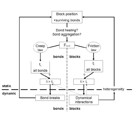
The different steps in this model are described in Figure 3. As explained previously, two phases are distinguished:

• A quasi-static phase corresponding to the nucleation of block sliding (Section 3.2) and bond rupture (Section 3.3).

• A dynamical phase corresponding to the sliding phase of the blocks (Section 3.4) and of the failure of bonds.

To account for the changes of the surface characteristics after blocks have slid, a random state parameter $\theta_{i}$ is assigned to each stopping block. In this way, the heterogeneity of the basal properties can be reproduced and is sustained during the evolution of the system.

4. Classification of the different regimes of gravity-driven instabilities

In a follow-up paper, we will apply the model presented in the previous section to case studies of the breaking-off of large ice masses of hanging glaciers, and in particular to the goal of understanding quantitatively the observations obtained for the Weisshorn hanging glacier [Faillettaz et al., 2008] and other glaciers in the Swiss Alps.

Here, we focus on the general properties of the model. We present a classification of the possible regimes that emerge as a result of the interplay between the different mechanisms, whose amplitudes are controlled by the parameter values.

4.1. Geometry and parameters

We consider a system of blocks, whose weights remain constant during the numerical simulation. This assumption is natural for modeling the nucleation phase preceding a rockslide or landslide. In the case of glaciers, this approximation is valid if the thickness of the glaciers is many times larger than the typical snow accumulation for a given year. For instance, in the case of the Weisshorn glacier with a thickness of about 30 meters, this assumption is well justified as, in addition, its northeastern face has a steep slope and is subjected to strong wind, which causes the snow to drift away.

In order to obtain a realistic description of the damage and fragmentation that may develop in a sliding mass, we need a sufficiently large number of blocks. As a compromise between reasonable sampling and computing time, we use a model composed of $600=20\times 30$ blocks for our numerical exploration of the different regimes.

In this vein, consider a glacier surface area of approximately $150\;\rm~{}m^{2}$, with a depth of 30 m. In a model composed of $20\times 30$ blocks, each block corresponds to a discrete mesh of size 30 m thickness, 5 m length and 5 m width. This implies that the weight of each block should be approximately equal to: $0.7\times 10^{6}\;\;\rm kg$ (with a density of $917\;\rm~{}kg\;m^{-3}$).

We study a particular geometry in which the slope is divided into two parts: Upper part stable (i.e., slope $<$ critical slope), lower part unstable (slope $>$ critical slope). Thus, the array is always driven towards an instability. Quantitatively, the slope $\phi$ of the underlying supporting surface, on which the mass is sliding ranges from $\phi_{\rm top}=45^{\circ}$ (upper part) to $\phi_{\rm bottom}=50^{\circ}$ (lower part). To account for the curvature of the slope, we used also a curved elevation of the supporting surface modeled by a portion of a parabola corresponding to a slope change from $45^{\circ}$ to $50^{\circ}$ over the size of the length of the glacier. We then chose a static friction parameter between $\tan 45^{\circ}$ and $\tan 50^{\circ}$, so that the upper part is in a frictional stable state, while the lower part is bound to start sliding. As a consequence of the slope change, the sliding of the lower part will transmit deformation and stress to the upper part. Our goal is to study this stress and deformation transfer and document the different regimes of sliding, rupture and fragmentation that occur as a function of the other model parameters.

The blocks are distributed in a regular mesh along the slope, in such a way that bonds are initially stress-free.

The following table summarizes the parameters used in our simulations and the values that are fixed throughout our numerical exploration of the different regimes.

Geometric parameters					Friction parameters
$n_{x}$	$n_{y}$	$m_{block}$	$l$	$\phi$	A	$\theta_{0}$	$\mu_{0}$	$\dot{\delta_{0}}$
-	-	[kg]	[m]	[∘]	-	[d]	-	[$\rm cm.d^{-1}$]
20	30	$2.75\times 10^{6}$	10	40 to 50	0.1		1	$10^{-3}$
Creep parameters
$E$	$\beta$	$C$	$\xi$	$e_{01}$	$e_{02}$
$[\rm Pa.m]$	[$\rm Pa^{-1}$]	[s]	-	-	-
			10	0.003	0.003

Table 1. Parameters used for the simulation. The mass has a total number of $n_{x}\times n_{y}$ blocks. The second row gives the list of parameters. The third row specifies the units of the parameters and the fourth row gives the numerical values used in the simulation for those parameters which have been fixed throughout. Missing entries correspond to the parameters that have been varied as explained in the text.

We find that the dependence of the mass evolution as a function of the other parameters can be reduced to a set of two reduced parameters.

1. The first important parameter is the elastic coefficient $E$ controlling the rigidity of the springs transferring stress between the blocks.

2. The second key parameter is the ratio $T_{c}/T_{f}$ of two characteristic time scales associated with the two fundamental processes: internal damage/creep and frictional sliding. The first time scale $T_{c}$ is associated with the creep-damage process occurring in the springs linking the blocks, also accounting for the natural frequency of the springs and reads

   (4.1) $$T_{c}=T\;\frac{\ln(\frac{C}{T})}{\beta~{}s^{\star}}~{},$$

   where $T$ is the natural period of the spring-mass system equal to $2\pi\sqrt{\frac{m_{block}}{E}}$, and where $C$, $\beta$ and $s^{\star}$ are three parameters of the creep-damage law defined by expressions (5.22), (5.12) and (5.21). Note that $\gamma$ in expression (5.23) reduces to $\beta$ since we assume for simplicity that $e_{02}=e_{01}$.
   The second time scale $T_{f}$ is associated with the frictional process controlling the tendency of blocks to slide and is derived from expression (5.11), leading to

   (4.2) $$T_{f}=\frac{\theta_{0}}{\exp(\frac{\tan(\phi_{\rm top})-\tan(\phi_{\rm bottom})}{A})-1}~{}.$$

   Here, $\theta_{0}$ and $A$ are two parameters of the friction law and $\phi_{\rm top}$ and $\tan(\phi_{\rm bottom})$ are the two angles of the unevenly slopping basal plane supporting the instable sliding mass.

Note that the first parameter $E$ has also an impact on $T_{c}$ through its effect on $s^{\star}$.

4.2. The three main regimes

4.2.1. Coherent sliding of the whole mass: $T_{c}/T_{f}$ large

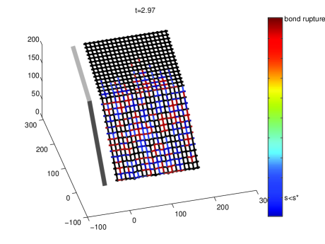
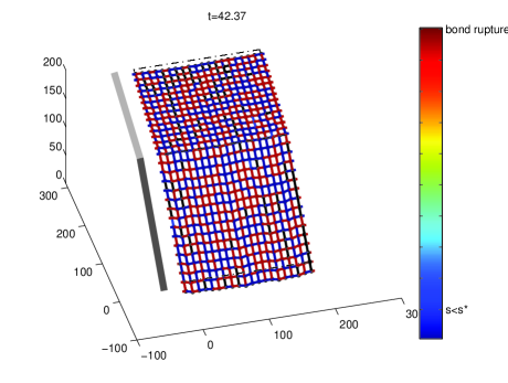
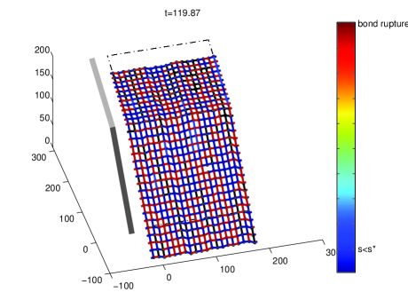
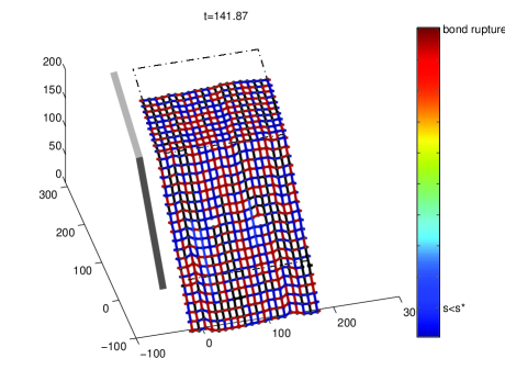
In this regime, the time needed for damage initiation is so great that the whole mass undergoes a series of internal stick and slip events, associated with an initial slow average downward motion of the whole mass. This average motion of the mass progressively accelerates until a global coherent run-away is observed. Specifically, we observe the following evolution:

1. First, the blocks in the lower part, where the slope is larger, start sliding intermittently in a stick-slip fashion.

2. The motion of these blocks transfers stress to the adjacent blocks, in turn leading to sliding events.

3. This dynamic evolves upstream, leading to an increasing number of blocks sliding in a stick-slip fashion.

4. The whole system is then undergoing stick-slip sliding, with increasing synchronization between the sliding blocks.

5. With increasing time, the system reaches a regime where a sufficiently large fraction of blocks are in the unstable lower part and the mass starts to slide as a whole, leading to a catastrophic coherent global slide.

This sequence is illustrated in Figure 4. This regime is observed at smaller values of $T_{c}/T_{f}$ for small elastic coefficient $E$. It is observed for large values of $E$ only for much larger ratios $T_{c}/T_{f}$ as shown in the phase diagram of Figure 13.

Figure 4. Illustration of the propagation of stick-slip events within the whole mass until it starts to slide coherently in a catastrophic runaway, occurring for large $T_{c}/T_{f}$ (i.e. $\sim 386$), for any $E$. Time increases from left to right and top to bottom. For the sake of simplicity, block are not drawn. The color of a bond evolves from black to red as the stress changes from lower than $s^{\star}$ to close to rupture.

Figure 5. Displacements and velocities of four selected blocks, one taken at the top of the slope ($y_{t}$), two near slope change ($y_{m1}$ and $y_{m2}$) and one at the bottom ($y_{t}$), in the stick-and-slip regime.

Figure 6. Kinetic energy for the stick-and-slip regime. The total number of surviving bonds is shown in the inset (solid line), as well as the number of surviving bonds in the upper (dashed and dotted line) and lower part (dashed line) of the model.

Figure 6 shows the time-dependence of four selected blocks, one in the upper region, two near the slope change and one in the lower region. After an initial phase, the velocity stabilizes and slightly increases as the whole mass slides downwards, where the slope is greater.

The inset in Figure 6 shows the number of surviving bonds as a function of time in the upper and lower parts. One observes that damage accumulates in the lower unstable sliding region, whereas the upper part remains basically undamaged. Figure 6 shows the kinetic energy of the moving blocks as a function of time. This graph gives an indication of the radiation energy emitted by cracks forming as a consequence of damage accumulation. In this regime, in which the whole mass evolves progressively towards a global coherent run-away sliding, one can observe a rich precursory behavior long before this unstable run-away occurs.

4.2.2. Fragmentation: $T_{c}/T_{f}$ small

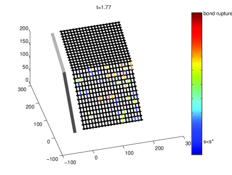
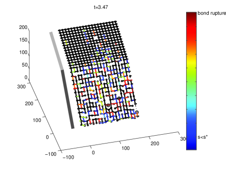
This regime has characteristics which are in a sense opposite to those of the previous regime: creep/damage occurs before the nucleation of sliding has time to develop, so that bonds break and the bottom part of the mass undergoes a fragmentation process with the creation of a heterogeneous population of sliding blocks. The typical evolution of the unstable mass is as follows:

1. First, the blocks in the lower part start sliding as in the previous case.

2. As previously, the deformation due to these sliding events propagates upstream, leading to stick-slip events.

3. Due to the relatively fast damage process, springs between blocks break, further increasing the stress, promoting further spring rupture, and so on.

4. Large fractured zones appear in the lower part, and blocks become isolated.

5. The final state is characterized by detached isolated blocks.

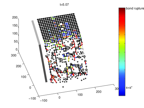
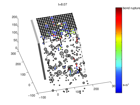
Four snapshots of the evolution of the mass illustrate this fragmentation process in Figure 7. This regime is observed for small values of $T_{c}/T_{f}$ and the large elastic coefficient $E$. It is observed for small values of $E$, ranging up to much larger ratios $T_{c}/T_{f}$, as shown in the phase diagram of Figure 13.

Figure 7. Illustration of the fragmentation process associated with sliding, occurring for small $T_{c}/T_{f}$(i.e. $\sim 1$), for any $E$. Diameters of the gray circles are proportional to the corresponding block mass (that change after aggregation process).

Figure 8. Displacements and velocities of four selected blocks, one taken at the top of the slope ($y_{t}$), two near slope change ($y_{m1}$ and $y_{m2}$) and one at the bottom ($y_{t}$), in the fragmentation regime.

Figure 9. Kinetic energy in the fragmentation regime. The total number of surviving bonds is shown in the inset (solid line), as well as the number of surviving bonds in the upper (dashed and dotted line) and lower part (dashed line) of the model.

Figure 9 shows the displacement and velocity of four selected blocks (same as Figure 6). Note that the blocks situated in the upper part do not slide. As soon as the blocks start sliding, their velocity increases. Generally speaking, this can be explained by bond rupture (as $T_{c}/T_{f}$ is small), meaning that the block is alone and does not interact anymore with its neighbors. The block accelerates according to equation (3.17) with F=0.

The figure 9 inset shows the time-dependence of the surviving bonds in the upper and lower parts. A very substantial level of damage can be observed, both in the lower and upper parts, in contrast with the previous regime. The damage level in the lower part leads to a completely fragmented mass. Figure 9 plots the time-dependence of the kinetic energy of the moving blocks. One can observe an intermittent kinetic energy that increases prior to full fragmentation, thus providing, as in the previous regime, an unambiguous precursory warning, albeit with a smaller advance time compared with the previous regime.

The kinetic energy increases due to isolated blocks moving downwards after the rupture of their bonds (this increase starts at t=7, see Figure 7). Because the system is already fragmented, this increase is of no use for an early warning. Radiated energy seems to provide a more reliable indication of early destabilization of the system.

4.2.3. Slab avalanche: $T_{c}/T_{f}\sim 1$

When neither damage nor frictional sliding dominates, an interesting phenomenon is observed: the occurrence of a macroscopic crack propagating roughly along the location of the largest curvature associated with the change of slope from the stable frictional state in the upper part to the unstable frictional sliding state in the lower part. The evolution of the mass proceeds as follows:

1. The first steps are similar to those observed in the two previous regimes, with individual blocks starting a stick-slip motion intermittently in the lower part.

2. The internal stresses created by these stick-slip events lead to an upstream propagation of these events, which progressively invades all the blocks in the lower part of the mass lying on the largest slope.

3. The damage time scale is such that the boost provided by the increased stress leads to a concentration of cracking at the boundary of the two slopes where the curvature is largest.

4. This leads to a nucleation and growth of a macroscopic crack which separates the mass into two parts.

5. The lower part evolves in a run-away situation with synchronized accelerating sliding, as in the first regime described in Section 4.2.1. The upper part remains largely untouched and stable.

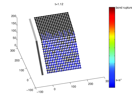
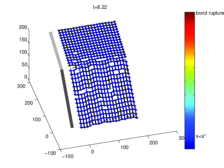
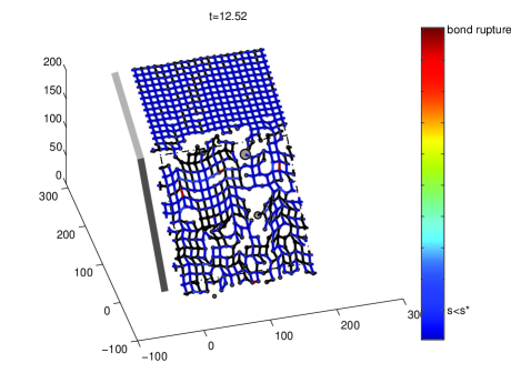
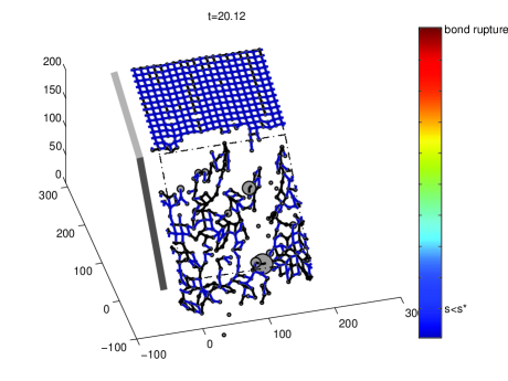
This regime is illustrated in four snapshots shown in Figure 10. It occurs in a band of large values of $T_{c}/T_{f}$ ratios, for the small enough elastic coefficient $E$, as shown in the phase diagram of Figure 13.

Figure 10. Illustration of slab avalanche process associated with sliding, occurring for intermediate $T_{c}/T_{f}$ (i.e. $\sim 25$). Diameters of the gray circles are proportional to the corresponding block mass (that change after aggregation process).

Figure 11. Displacements and velocities of four selected blocks, one taken at the top of the slope ($y_{t}$), two near slope change ($y_{m1}$ and $y_{m2}$) and one at the bottom ($y_{t}$), in the slab avalanche transition regime.

Figure 12. Kinetic energy, in the slab avalanche transition regime. The total number of surviving bonds is shown in the inset (solid line), as well as the number of surviving bonds in the upper (dashed and dotted line) and lower part (dashed line) of the model.

The Figure 12 inset shows the number of surviving bonds as a function of time in the upper and lower part. Most of the damage occurs in the lower unstable sliding region. It can be observed that the fraction of surviving bonds drops suddenly after the nucleation time (here about $13$ days) of the macroscopic crack separating the lower from the upper parts. Figure 12 shows the time evolution of the kinetic energy of the moving blocks. Compared with previous regimes, there is a much shorter (if any) advance warning time, which is compatible with the first-order nature of the nucleation of a macroscopic crack.

4.3. Phase diagram in the plane $[E;T_{c}/T_{f}]$

Figure 13. Phase diagram in the plane $[E;T_{c}/T_{f}]$ summarizing the three main regimes identified. The transition between the “stick-slip transition to global runaway” and the “fragmentation” regimes is continuous. The intermediate regime is characterized by the occurrence of a macroscopic slab avalanche (closed to the unstable behaviour) or global instability (closed to the stable one). The existence of heterogeneities is found to play an important role in the transitional behavior. Fragmentation ($\diamond$), stick-slip ($\times$) and slab avalanche ($+$) regimes are indicated.

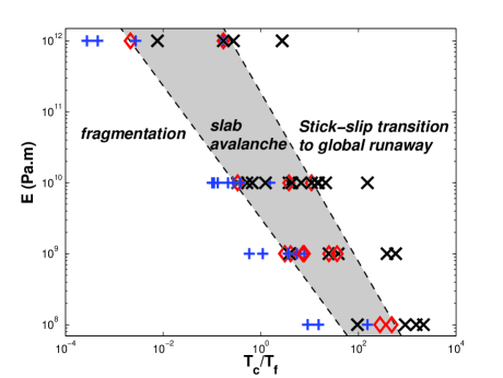
These three regimes are summarized in the phase diagram in the plane $[E;T_{c}/T_{f}]$ shown in Figure 13.

The elastic coefficient $E$ ($=Y\times l$) controls the global deformation of the array of block-springs. Small $E$-values lead to large block displacements as well as large deformation of the system. In contrast, for large $E$-values, the block displacements are small and the deformations are therefore small too. A large rigidity favors the emergence of a coherent behavior of the block motion. $E$ can be understood as controlling the correlation length of displacements in the system. A larger $E$-value leads to larger clusters of blocks sliding simultaneously in local avalanches. The upstream propagation of the stick-slip motion is facilitated and develops faster for larger $E$’s.

The “slab avalanche” transition regime is found for intermediate values of $T_{c}/T_{f}$, resulting from the competition of instabilities between basal friction and crack formations. This regime is sensitive to the presence of heterogeneities. They are modeled by the random resetting of the state variable $\theta_{i}$ of the frictional process after each sliding event.

5. Conclusion

With the goal of developing a better understanding of the physical mechanisms leading to accelerated motions and to increasing seismic activity reported in the case of gravity-driven instabilities, we have developed a numerical model based on the discretization of the natural medium in terms of blocks and springs forming a two-dimensional network sliding on an inclined plane. Each block, which can slide, is connected to its four neighbors by springs, that can fail, depending on the history of displacements and damage. We develop physically realistic models describing the frictional sliding of the blocks on the supporting surface and the tensile failure of the springs between blocks proxying for crack opening. Frictional sliding is modeled with a state-and-velocity weakening friction law with threshold. Crack formation is modeled with a time-dependent cumulative damage law with thermal activation including stress corrosion. In order to reproduce cracking and dynamical effects, all equations of motion (including inertia) for each block are solved simultaneously.

The numerical exploration of the model shows the existence of three regimes as a function of the ratio $T_{c}/T_{f}$, which are the two characteristic time scales associated with the two fundamental processes (internal damage/creep and frictional sliding). For $T_{c}/T_{f}\gg 1$, the whole mass undergoes a series of internal stick and slip events, associated with an initial slow average downward motion of the whole mass which progressively accelerates until a global coherent run-away is observed. For $T_{c}/T_{f}\ll 1$, creep/damage occurs faster than nucleation of sliding, bonds break and the bottom part of the mass undergoes a fragmentation process with the creation of a heterogeneous population of sliding blocks. For the intermediate regime $T_{c}/T_{f}\sim 1$, a macroscopic crack forms and propagates along the location of the largest curvature associated with the slope change. In the upper part above the crack, the stable frictional state prevails, while in the lower part, the unstable frictional sliding state dominates.

Our framework allows for the first time the combination of competing frictional and damage processes at the origin of mass instabilities. It clears the path to a better understanding of rupture mechanisms in heterogeneous media. It also casts a gleam of hope for better forecasting of the ultimate rupture of gravity-driven systems. Calibrating the relevant physical parameters to different natural materials (soil, rocks, ice or snow) will also help in the investigation of the slope stability under external forcing conditions (such as climate changes).

Appendix A: Initiation of sliding for a single block

This appendix complements Section 3.2 by providing details of the calculation of the critical time at which unstable sliding of a given block occurs. Section 3.2 describes the sub-critical sliding process of a given block interacting via state-and-velocity solid friction with its inclined basal surface. When the sub-critical sliding velocity $d\delta/dt$ diverges (we refer to the time when this occurs as the “critical time” $t_{f}$ for the frictional sliding instability), this signals a change of regime to the dynamical sliding regime where inertia (the block mass and its acceleration in the Newton’s law) has to be taken into account.

Let us calculate explicitly how the critical time $t_{f}$ is obtained and define its dependence on the parameters and boundary conditions. Let us call $T\equiv\Arrowvert\sum\vec{F}_{\rm bond}\;-\;T_{\rm weight}\vec{x}\Arrowvert$ (or $N\equiv N_{\rm weight}$) the total shear (or normal) force exerted on a given block, where $\vec{F}_{\rm bond}$ is the force exerted by a neighboring spring bond, and $N_{\rm weight}$ and $T_{\rm weight}$ are the normal and tangential forces due to the weight of the block. We then have

(5.1) $$\mu=\frac{T}{N}=\tan\phi~{},$$

where $\phi$ is the angle of the basal surface supporting the block. Therefore,

(5.2) $$\mu_{0}+A\;\ln\frac{\dot{\delta}}{\dot{\delta}_{0}}+B\;\ln\frac{\theta}{\theta_{0}}=\tan\phi~{}.$$

As explained in Section 3.2, $A-B$ is usually very small for natural material, of the order of $A-B\approx\pm 0.02$. For the sake of simplicity, we assume $A=B$. As recalled in Section 3.2, this choice is not restrictive as it recovers the two important regimes [Helmstetter et al., 2004]. This leads to

(5.3) $$\ln\;\frac{\dot{\delta}}{\dot{\delta_{0}}}\frac{\theta}{\theta_{0}}\;=\;\frac{\tan\phi-\mu_{0}}{A}$$

whose solution is

(5.4) $$\dot{\delta}.\theta\;=\;(\dot{\delta}_{0}\;\theta_{0})\;\exp\left(\frac{\tan\phi-\mu_{0}}{A}\right)~{}.$$

From Equation (3.2), we have

(5.5) $$\dot{\theta}=1-\frac{\theta\;\dot{\delta}}{D_{c}}=1-{\;\dot{\delta}_{0}\;\theta_{0}\over D_{c}}~{}\exp\left(\frac{\tan\phi-\mu_{0}}{A}\right)$$

Then

(5.6) $$\theta\;=\;\theta_{0}+\Big{(}1-\frac{\;(\dot{\delta}_{0}\;\theta_{0})\;\exp\left(\frac{\tan\phi-\mu_{0}}{A}\right)}{D_{c}}\Big{)}t$$

and using Equation (5.4), we obtain

(5.7) $$\dot{\delta}~{}=~{}{\;(\dot{\delta}_{0}\;\theta_{0})\;\exp\left(\frac{\tan\phi-\mu_{0}}{A}\right)\over\theta_{0}+\Big{(}1-{\;\dot{\delta}_{0}\;\theta_{0}\over D_{c}}\;\exp\left(\frac{\tan\phi-\mu_{0}}{A}\right)\Big{)}t}~{}.$$

This expression exhibits the usual regimes: a finite time singularity is obtained for $\;(\dot{\delta}_{0}\;\theta_{0})\;\exp\left(\frac{\tan\phi-\mu_{0}}{A}\right)>D_{c}$. In this case, Expression (5.7) can be re-written as

(5.8) $$\dot{\delta}\;={D_{c}\;\dot{\delta}_{0}\;\theta_{0}\;\exp\left(\frac{\tan\phi-\mu_{0}}{A}\right)\over D_{c}-\dot{\delta}_{0}\;\theta_{0}\;\exp\left(\frac{\tan\phi-\mu_{0}}{A}\right)}\cdot{1\over t_{f}-t}$$

with

(5.9) $$t_{f}\;=\;{D_{c}\theta_{0}\over D_{c}-\dot{\delta}_{0}\;\theta_{0}\;\exp\left(\frac{\tan\phi-\mu_{0}}{A}\right)}~{}.$$

We can simplify Expression (5.8) by using the condition that, for $\mu=\tan\phi=\mu_{0}$, we should have $t_{f}\rightarrow\infty$. But, for $\mu=\mu_{0}$, $\exp\left(\frac{\mu_{s}-\mu_{0}}{A}\right)=1$ and thus, for the condition $t_{f}\to\infty$ to hold, we need

(5.10) $${\dot{\delta}_{0}\;\theta_{0}\over D_{c}}=1~{}.$$

The final expression for the critical time $t_{f}$ signaling the transition from a subcritical sliding to the dynamical inertial sliding is, for $\mu>\mu_{0}$,

(5.11) $$t_{f}\;=\;\frac{\theta_{0}}{\exp(\frac{\mu_{s}-\mu_{0}}{A})-1},$$

while $t_{f}\to\infty$ for $\mu\leq\mu_{0}$. Note that the dependence on $\dot{\delta_{0}}$ has disappeared due to the relation (5.10).

To summarize, a given configuration of blocks and spring tensions determines the value of $T\equiv\Arrowvert\sum\vec{F}_{\rm bond}\;-\;T_{\rm weight}\vec{x}\Arrowvert$ and $N\equiv N_{\rm weight}$ and therefore of $\mu$ via (5.1). Knowing $\mu$ and given the other material parameters $\theta_{0},\mu_{0}$ and $A$, we determine the time $t_{f}$ for the transition to the dynamical regime for that block via Equation (5.11).

Appendix B: Determination of the rupture time $t_{c}$ for a single bond

Case of a constant applied stress up to rupture

Combining Equations (3.8), (3.9) and (3.10) in section 3.3 yields

(5.12) $$\frac{de}{dt}=K\sinh\Bigg{(}\frac{\beta\;s\;}{e_{01}^{\mu}}(e+e_{02})^{\mu}\;-\;\beta Ee\Bigg{)}$$

for the equation governing the deformation $e$ of a bond subjected to an applied stress $s$.

Nechad et al. [2005] have studied both analytically and numerically the solution of this equation (5.12) in the case $s>s^{*}$ (where $s^{*}$ is defined in the main text) for which the deformation $e$ blows up to infinity in finite time $t_{c}$, reflecting the accelerated tertiary creep regime culminating in the global rupture of the bond.

Our purpose here is to provide a simple approximate formula for the rupture time $t_{c}$, which will be used in numerical simulations of the global dynamics of the block array.

An initial method to obtain $t_{c}$ uses an approximate expression interpolating between the time evolution of $e(t)$ far from and close to $t_{c}$ found by Nechad et al. [2005]. We propose the expression

(5.13) $$e(t)\;=\;\mathcal{A}\;ln(\mathcal{B}+\mathcal{C}t)\Big{[}-\ln(\frac{t_{c}-t}{\tau})\Big{]}^{\frac{1}{\mu}}\;\;,$$

where $\mathcal{A}$,$\mathcal{B}$, $\mathcal{C}$, $t_{c}$ and $\tau$ are constants to be determined from matching conditions far from and close to $t_{c}$. In particular, Nechad et al. [2005] shows that for $t\ll t_{c}$, Equation (5.12) simplifies into

(5.14) $$\frac{de}{dt}\;=\;\frac{a}{b+ct}$$

with $a=Ke_{02}$, $b=2e_{02}\;\exp(-\beta s(\frac{e_{02}}{e_{01}})^{\mu})$ and $c=K\beta\;(Ee_{02}-\mu s(\frac{e_{02}}{e_{01}})^{\mu})$, while for $t\approx t_{c}$, expression (5.12) simplifies into

(5.15) $$\frac{de}{dt}\;=\;\frac{d}{\mu}\;\Big{[}-\ln(t_{c}-t)\Big{]}^{(1/\mu)-1}\;\frac{1}{t_{c}-t}$$

with $d\;=\;e_{01}(\beta s)^{-1/\mu}$.

We expand expression (5.12) for $t\ll t_{c}$and for $t\to t_{c}$ and identify with Equations (5.14) and (5.15) respectively to obtain the system of five equations for the five unknown $\mathcal{A}$,$\mathcal{B}$, $\mathcal{C}$, $t_{c}$ and $\tau$:

(5.16) $$\left\{\begin{array}[]{rcl}e_{0}&=&\mathcal{A}\;\ln\mathcal{B}\;\Big{(}-\ln\frac{t_{c}}{\tau}\Big{)}^{\frac{1}{\mu}}\;\;,\\ &&\qquad\qquad\qquad\qquad{\rm for}\;\;t\ll t_{c}\;\;\;e(t=0)=e_{0}\\ \frac{a}{b}&=&\mathcal{A}\;\Big{(}-\ln\frac{t_{c}}{\tau}\Big{)}^{\frac{1}{\mu}-1}\;\Bigg{(}\mathcal{B}\mathcal{C}\Big{(}-\ln\frac{t_{c}}{\tau}\Big{)}+\frac{\tau\ln\mathcal{B}}{\mu t_{c}}\Bigg{)}\;\;,\\ &&\qquad\qquad\qquad\qquad{\rm for}\;\;t\ll t_{c}\;\;\;t^{0}\\ -\frac{ac}{b^{2}}&=&\mathcal{A}\;\Big{(}-\ln\frac{t_{c}}{\tau}\Big{)}^{\frac{1}{\mu}-1}\;\Bigg{(}-\mathcal{C}^{2}\Big{(}-\ln\frac{t_{c}}{\tau}\Big{)}+\frac{\tau\mathcal{C}}{\mu t_{c}\mathcal{B}}\Bigg{)}\;\;,\\ &&\qquad\qquad\qquad\qquad{\rm for}\;\;t\ll t_{c}\;\;\;t^{1}\\ \frac{ac^{2}}{b^{2}}&=&\mathcal{A}\;\Big{(}-\ln\frac{t_{c}}{\tau}\Big{)}^{\frac{1}{\mu}-1}\;\Bigg{(}\frac{\mathcal{C}^{2}}{\mathcal{B}}\Big{(}-\ln\frac{t_{c}}{\tau}\Big{)}-\frac{\tau\mathcal{C}^{2}}{2\mu t_{c}\mathcal{B}^{2}}\Bigg{)}\;\;,\\ &&\qquad\qquad\qquad\qquad{\rm for}\;\;t\ll t_{c}\;\;\;t^{2}\\ \frac{d\tau}{\mu t_{c}}&=&\mathcal{A}\;\Bigg{[}\frac{\mathcal{C}}{\mathcal{B}+\mathcal{C}t_{c}}\Big{(}-\ln\frac{t_{c}}{\tau}\Big{)}+\frac{\tau\;\ln(\mathcal{B}+\mathcal{C}t_{c}}{\mu t_{c}}\Bigg{]}\;\;,\\ &&\qquad\qquad\qquad\qquad{\rm for}\;\;t\approx t_{c}\;\;\;(t_{c}-t)^{0}.\end{array}\right.$$

While this system should allow us in principle to determine $t_{c}$, its nonlinearity makes it unwieldy. We propose an alternative approach, which consists in first simplifying Equation (5.13) for $t\ll t_{c}$ and $t\approx t_{c}$:

• For $t\ll t_{c}$:

  (5.17) $$\frac{de}{dt}\;=\;\frac{\mathcal{A}\mathcal{C}}{\mathcal{B}+\mathcal{C}t}\;\Bigg{[}-\ln\Big{(}\frac{t_{c}}{\tau}\Big{)}\Bigg{]}^{\frac{1}{\mu}}$$

• for $t\approx t_{c}$:

  (5.18) $$\frac{de}{dt}\;=\;\mathcal{A}\;\ln(\mathcal{B}+\mathcal{C}t_{c})\frac{1}{\mu}\;.\;\frac{1}{t_{c}-t}\Bigg{[}-\ln\Big{(}\frac{t_{c}-t}{\tau}\Big{)}\Bigg{]}^{\frac{1}{\mu}-1}$$

In this approach, it is consistent to put $\tau$ equal to $\frac{1}{K}$ where $K$ is the constant defined in equation (3.8). Identification with equations (5.14) and (5.15) gives the following system:

(5.19) $$\left\{\begin{array}[]{rcl}a&=&\mathcal{A}\mathcal{C}\;\Big{[}-\ln\frac{t_{c}}{\tau}\Big{]}^{\frac{1}{\mu}}\;\;,\\ b&=&\mathcal{B}\;\;,\\ c&=&\mathcal{C}\;\;,\\ d&=&\mathcal{A}\;\ln(\mathcal{B}+\mathcal{C}t_{c})\;\;.\end{array}\right.$$

Eliminating $\mathcal{A}$ in (5.19) yields an implicit equation that determines $t_{c}$:

(5.20) $$\left[-\ln\frac{t_{c}}{\tau}\right]^{1/\mu}\;\frac{1}{\ln(b+ct_{c})}=\frac{a}{cd}$$

This implicit equation is found to be sensitive to the value of the initial parameters and its use is still rather computer-intensive, which makes it inconvenient for simulations involving large systems with many blocks.

We have thus turned to a simpler but more approximate method, using the asymptotic analytical results obtained in Nechad et al. [2005] that, for $s\gg s^{*}$ where

(5.21) $$s^{\star}=E\;\;\Big{(}\frac{e_{01}}{\mu}\Big{)}^{\mu}\;\;\Big{(}\frac{\mu-1}{e_{02}}\Big{)}^{\mu-1}$$

is the minimum stress such that the material will fail eventually, $t_{c}$ is given by

(5.22) $$t_{c}=C\;\exp(-\gamma\;s)~{},$$

where

(5.23) $$\gamma=\frac{\beta e_{02}^{\mu}}{e_{01}^{\mu}}~{}.$$

As $K$ has the dimension of the inverse of time in Equation (5.12), we take the constant $C$ to be proportional to $1/K$: $C\sim\frac{1}{K}$. Our formula for determining $t_{c}$ in our simulations is therefore summarized by the following equations:

(5.24) $$t_{c}=\left\{\begin{array}[]{ll}{1\over K}\;\exp(-\gamma\;s)&\textrm{if }s>s^{\star}\\ \to\infty&\textrm{if }s\leq s^{\star}\end{array}\right.$$

6. Appendix C: Energy analysis

In order to analyze our results in term of icequake activity and compare numerical with experimental results, we estimate the energy evolution in the lattice. Here, four types of energy can be distinguished and evaluated: gravitational potential energy, kinetic energy, energy stored in the elastic bonds (analogous to an internal energy) and radiated energy.

Gravitational potential energy

The gravitational potential energy is evaluated using the classical expression:

(6.1) $$E_{p}(t)\;=\;\sum_{all\;\;blocks}mg\;\;z_{block}$$

Energy stored in bonds

For each bond linking block $i$ and block $j$, the stored elastic energy is defined by:

(6.2) $$E_{b}(t)=\frac{1}{2}\sum_{all\;\;bonds}E\Big{(}b_{ij}\Arrowvert\vec{x}_{j}-\vec{x}_{i}\Arrowvert-l\Big{)}^{2}$$

where $\vec{x}_{j}$ and $\vec{x}_{i}$ are the position of two neighboring blocks and $l$ the initial length of each bond.

Kinetic energy

The total kinetic energy of the system is evaluated according to the formula

(6.3) $$E_{k}(t)=\sum_{all\;\;blocks}\frac{1}{2}m\Big{(}\frac{\Arrowvert\vec{x}(t+\delta t)-\vec{x}(t)\Arrowvert}{\delta t}\Big{)}^{2}$$

with $\vec{x}(t)$ the position of the considered block at time $t$.

Radiated energy

The radiated energy $E_{r}(t)$ between two time steps is evaluated using:

(6.4) $$E_{r}(t)\;=\;E_{t}-E_{p}(t)-E_{b}(t)-E_{k}(t)$$

with $E_{t}=E_{p}(0)+E_{b}(0)+E_{k}(0)=E_{p}(0)$. In other words, it is the additional energy not found in the potential, elastic or kinetic energies.

References

- [1] Abele, G. (1974). Bergstürze in den Alpen. Ihre Verbreitung, Morphologie und Folgeerscheinungen. Wissensch. Alpenverreinshefte, 25, München.
- [2] Al-Homoud, A.S. and Tahtamoni, W.W. (2001). A reliability based expert system for assessment and mitigation of landslides hazard under seismic loading, Natural Hazards 24, 13-51.
- [3] Amitrano, D., Grasso J.-R. and Senfaute, G. (2005). Seismic precursory patterns before a cliff collapse and critical point phenomena, Geophysical Research Letters, 32:L08314.
- [4] Andersen, J.V., D. Sornette and K.-T. Leung (1997). Tri-critical behavior in rupture induced by disorder, Phys. Rev. Lett. 78, 2140-2143.
- [5] Anifrani, J.-C., C. Le Floc’h, D. Sornette and B. Souillard (1995). Universal Log-periodic correction to renormalization group scaling for rupture stress prediction from acoustic emissions, J.Phys.I France 5, 631-638.
- [6] Azzoni, A., Chiesa, S., Frassoni, A. and Govi, M. (1992). The Valpola landslide, Eng. Geol., 33, 59-70.
- [7] Ben-Zion, Y. (2001). Dynamic ruptures in recent models of earthquake faults, Journal of the Mechanics and Physics of Solids, 49, 2209-2244.
- [8] Ben-Zion, Y. (2003). Key formulas in earthquake seismology, International Handbook of Earthquake and Engineering Seismology, vol. 81B.
- [9] Ben-Zion, Y. and J.R. Rice (1997). Dynamic simulations of slip on a smooth fault in an elastic solid, J. Geophys. Res., 102, 17771-17784.
- [10] Berardino, P., M. Costantini, G. Franceschetti, A. Iodice, L. Pietranera and V. Rizzo (2003). Use of differential SAR interferometry in monitoring and modelling large slope instability at Maratea (Basilicata, Italy), Engineering Geology, 68 (1-2), 31-51.
- [11] Berger, E.J. (2002). Friction Modeling for Dynamic System Simulation, Applied Mechanics Reviews, 55 (6),535.
- [12] Bhandari R.K. (1988). Some lessons in the investigation and field monitoring of landslides, Proceedings 5th Int. Symp. Landslides lausanne 1988, eds C. Bonnard , vol 3, 1435-1457, Balkema.
- [13] Blake, T.F., R.A. Hollingsworth and J.P. Stewart, editors (2002). Recommended Procedures for Implementation of DMG Special Publication 117, Guidelines for Analyzing and Mitigating Landslide Hazards in California, Committee organized through the ASCE Los Angeles Section Geotechnical Group, Document published by the Southern California Earthquake Center.
- [14] Bowman, D.D., G. Ouillon, C.G. Sammis, A. Sornette and D. Sornette (1998). An Observational test of the critical earthquake concept, J.Geophys. Res. 103, (NB10), 24359-24372.
- [15] Brabb, E.E. (1991). The world landslide problem, Episodes 14, 52-61.
- [16] Brunsden, D. (1999) Some geomorphological considerations for the future development of landslide models, Geomorphology, 30, 13-24.
- [17] Bufe, C. G. and Varnes, D. J. (1993). Predictive modeling of the seismic cycle of the greater San Francisco Bay area, J. Geophys. Res. B 98, 9871-9883.
- [18] Campbell, C.S. (1989). Self-lubrification for long runout landslides, J. Geolo. 97, 653-665.
- [19] Campbell, C.S. (1990). Rapid granular flow, Annu. Rev. of Fluid Mech., 22, 57-92.
- [20] Campbell, C.S., P.W. Cleary and M. Hopkins (1995). Large-scale landslide simulations - Global deformation, velocities and basal friction, J. Geophys. Res., 100 (NB5), 8267-8283.
- [21] Caplan-Auerbach, J., Fox, C.G. and Duennebier, F.K. (2001). Hydroacoustic detection of submarine landslides on Kilauea volcano, Geophys. Res. Letts, 28, 1811-1813.
- [22] Chau, K.T. (1995). Landslides modeled as bifurcations of creeping slopes with nonlinear friction law, Int. J. Solids Struct., 32, 3451-3464.
- [23] Chau, K.T. (1999). Onset of natural terrain landslides modelled by linear stability analysis of creeping slopes with a two state friction law, International journal for numerical and analytical methods in geomechanics, 23, 1835-1855.
- [24] Ciliberto, S., Guarino A., Scorretti, R. (2001). The effect of disorder on the fracture nucleation process, Physica D 158 (1-4), 83-104.
- [25] Cleary, P.W. and C.S. Campbell (1993). Self-lubrication for long runout landslides - Examination by computer simulations, J. Geophys. Res., 98 (NB12), 21911-21924.
- [26] Clouard, V. Bonneville, A., Gillot, P.Y. (2001). A giant landslide on the southern flank of Tahiti Island, French Polynesia, Geophys. Res. Letts., 28, 2253-2256.
- [27] Coe, J.A., W.L. Ellis, J.W. Godt, W.Z. Savage, J.E. Savage, J.A. Michael and J.D. Kibler, P.S. Powers, D.J. Lidke and S. Debray (2003). Seasonal movement of the Slumgullion landslide determined from Global Positioning System surveys and field instrumentation, July 1998-March 2002, Engineering Geology, 68 (1-2), 67-101.
- [28] Colesanti, C., A. Ferretti, C. Prati and F. Rocca (2003). Monitoring landslides and tectonic motions with the Permanent Scatterers Technique, Engineering Geology, 68 (1-2), 3-14.
- [29] Cruden, D.M. (1997). Report of the International Workshop on Landslide Risk Assessment – Honolulu, Hawaii, USA, 19-21 February, 1997 (1997) Episodes 20, 264-264.
- [30] Davis, R.O., Smith, N.R., Salt, G. (1990). Pore fluid frictional heating and stability of creeping landslides, Int. J. Num. Anal. Meth. Geomechanics, 14, 427-443.
- [31] Dieterich, J.H. (1994). A constitutive law for rate of earthquake production and its application to earthquake clustering, J. Geophys. Res. 99, 2601-2618.
- [32] Eisbacher, G.H. (1979). Cliff collapse and rock avalacnhes in the Mackenzie Mountains, Northwestern Canada, Can. Geot. J., 16, 309-334.
- [33] Erismann, T. and Abele, G. (2001). Dynamics of rockslides and rockfalls (Berlin;New York: Springer).
- [34] Faillettaz, J., Pralong, A., Funk, M. and Deichmann, N. (2008). Evidence of log-periodic oscillations and increasing icequake activity during the breaking-off of large ice masses. Journal of Glaciology, 57, (187), 725.
- [35] Farkas, Z., Dahmen S.R. and Wolf D.E. (2005). Static versus dynamic friction: the role of coherence Journal of Statistical Mechanics: Theory and Experiment, 6, P06015
- [36] Flotron, A. (1977). Movement studies on hanging glaciers in relation with an ice avalanche, Journal of Glaciology, 19 (81): 671–672.
- [37] Fruneau, B., Achache, J. and Delacourt, C. (1996). Observation and modelling of the Saint-Etienne-de-Tinée landslide using SAR interferometry, Tectonophysics 265, 181-190.
- [38] Fukuzono, T. (2000). Recent studies on time prediction of slope failure, Landslide News, 4, 9-12.
- [39] Gluzman, S. and D. Sornette (2001). Self-Consistent Theory of Rupture by progressive diffuse damage, Physical Review E V63 06 N6 PT2:6129, U241-U250.
- [40] Gomberg, J., Beeler, N. and Blanpied, M. (2000). On rate-state and Coulomb failure models, J. Geophys. Res. 105 NB4, 7857-7871.
- [41] Gomberg, J., Bodin, P., Savage, W. and Jackson, M.E. (1995). Landslide faults and tectonic faults, Analogs? – The slumgullion earthflow, Colorado (1995) Geology 23, 41-44.
- [42] Goretta, K. C., Cruse, T. A., Koritala, R. E., Routbort, J. L., Mélendez-Martínez, J. J., de Arellano-López, A. R., (2001). Compressive creep of polycrystalline ZrSiO4, Journal of the European Ceramic Society, 21 (8), 1055-1060.
- [43] Guarino, A., Ciliberto, S., Garcimartin, A. Zei, M., Scorretti, R., (2002). Failure time and critical behaviour of fracture precursors in heterogeneous materials, Eur. Phys. J. B. 26 (2), 141-151.
- [44] Guzzetti, F., Carrara, A., Cardinali, M. and Reichenbach, P. (1999). Landslide hazard evaluation: a review of current techniques and their application in a multi-scale study, Central Italy, Geomorphology 31, 181-216.
- [45] Heim, A. (1932). Bergsturz und Menschenleben, Fretz und Wasmuth, Zürich.
- [46] Heinrich, P., Guibourg, S., Mangeney, A. and Roche, R. (1999). Numerical modeling of a landslide-generated tsunami following a potential explosion of the Montserrat volcano, Phys.Chem. Earth A 24, 163-168.
- [47] Helmstetter, A., D. Sornette, J.-R. Grasso, J. V. Andersen, S. Gluzman and V. Pisarenko (2004). Slider-Block Friction Model for Landslides: Application to Vaiont and La Clapiere Landslides, J. Geophys. Res., 109, B02409, doi:10.1029/2002JB002160.
- [48] Hidalgo, R.C., Kun, F., Herrmann, H.J., (2002). Creep rupture of viscoelastic fibre bundles, Phys. Rev. E. 65 (3), 032502/1-4.
- [49] Hoek, E. and J.Bray (1981). Rock slope engineering, 3rd ed., London, Institution of Mining and Metallurgy.
- [50] Howell, D.G., Brabb, E.E. and Ramsey, D.W. (1999). How useful is landslide hazard information? Lessons learned in the San Francisco Bay Region, International Geology Review 41, 368-381.
- [51] Hurlimann, M., Marti, J, and Ledesma, A. (2000). Mechanical relationship between catastrophic volcanic landslides and caldera collapses, Geophys. Res. Lett. 27, 2393-2396.
- [52] Ide, K. and D. Sornette (2002). Oscillatory Finite-Time Singularities in Finance, Population and Rupture, Physica A 307 (1-2), 63-106.
- [53] Ishikawa, K., Maehara, M., Kobayashi. Y. (2002). Mechanical modeling and microstructural observation of pure aluminum crept under constant stress, Materials Science and Engineering A322 (1-2), 153-158.
- [54] Iverson, R.M. (1985). A constitutive equation for mass-movement behavior, Journal of Geology, 93, 143-160.
- [55] Iverson, R.M. (1986a). Unsteady, nonuniform landslide motion: 1. Theoretical dynamics and the steady datum state, Journal of Geology, 94, 1-15.
- [56] Iverson, R.M. (1986b). Unsteady, nonuniform landslide motion: 2. Linearized theory and the kinematics of transient response, Journal of Geology, 94, 349-364.
- [57] Iverson, R.M. (1993). Differential equations governing slip-induced pore-pressure fluctuations in a water-saturated granular medium, Mathematical Geology, 25 (8), 1027-1048.
- [58] Iverson, R.M. et al.(2000) .
- [59] Iverson, R.M. and M.E. Reid (1992). Gravity-driven groundwater flow and slope failure potential. 1. Elastic effective-stress model, Water Resources Research, 28 (3), 925-938.
- [60] Jaumé, S. C. and Sykes, L. R. (1999). Pure Appl. Geophys. 155, 279-306.
- [61] Johansen, A. and D. Sornette (1999). Acoustic radiation controls dynamic friction: Evidence from a spring-block experiment, Physical Review Letters 82(25), 5152-5155.
- [62] Johansen, A. and D. Sornette (2001). Finite-time singularity in the dynamics of the world population and economic indices, Physica A 294 (3-4), 465-502.
- [63] Kilburn, C.R.J., and D.N. Petley D.N. (2003). Forecasting giant, catastrophic slope collapse: lessons from Vajont, Northern Italy, Geomorphology, 54, 21-32.
- [64] Korner, H.J. (1976). Reichweite and Geschwindigkeit von Bergsturzen und Fleisscheneelawinen, Rock mechanics, 8, 2256-256.
- [65] Kuhn, M.R. and J.K. Mitchell (1993). New perspective on soil creep, J. Geotechnical Engineering, 119 (3), 507-524.
- [66] Kun, F., Moreno, Y., Hidalgo, R.C., Herrmann, H.J., 2003. Creep rupture has two universality classes, Europhysics Letters 63 (3), 347-353.
- [67] Lapusta N., J.R. Rice, Y. Ben-Zion, G. Zheng (2000). Elastodynamic analysis for slow tectonic loading with spontaneous rupture episodes on faults with rate- and state-dependent friction, J. Geophys. Res. 105 (B10) (Solid Earth), 23765-2389.
- [68] Leung, K. and J.V. Andersen (1997). Phase transition in a spring-block model of surface fracture, Europhysics Letters, 38 (8), 589-594.
- [69] Liu, J.Y., Ross, R.J. (1996). Energy criterion for fatigue strength of wood structural members, Journal of Engineering Materials and Technology 118 (3), 375-378.
- [70] Lockner, D. A. (1998). A generalized law for brittle deformation of Westerly granite, J. Geophys. Res. 103 (B3), 5107-5123.
- [71] Lüthi, M. (2003). Instability in glacial systems, Milestones in Physical Glaciology: From the Pioneers to a Modern Science, 180, 63–70, VAW, ETH-Zürich.
- [72] Main, I. G. (2000). A damage mechanics model for power-law creep and earthquake aftershock and foreshock sequences, Geophys. J. Int. 142(1), 151-161.
- [73] Malet, J.P., Maquaire, O. and Calais, E. (2002). The use of Global Positioning System techniques for the continuous monitoring of landslides: application to the Super-Sauze earthflow (Alpes-de-Haute-Provence, France), Geomorphology 43, 33-54.
- [74] Mantovani, F., Soeters, R. and Vanwesten, C.J. (1996). Remote sensing techniques for landslide studies and hazard zonation in Europe, Geomorphology 15, 213-225.
- [75] Marone, C. (1998). Laboratory-derived friction laws and their application to seismic faulting, Ann. Rev. Earth Planet. Sci. 26, 643-696.
- [76] McMurtry, G.M., Herrero-Bervera, E., Cremer, M.D., Smith, J.R., Resig, J., Sherman, C., and M.E. Torresan (1999). Stratigraphic constraints on the timing and emplacement of the Alika 2 giant Hawaiian submarine landslide. J. Vol. Geother. Res. 94, 35-58.
- [77] Meakin, P. (1991). Models for material failure and deformation, Science 252, 226-234.
- [78] Miguel, M.C., Vespignani, A. Zaiser, M. Zapperi, S. (2002). Dislocation jamming and Andrade creep, Phys. Rev. Lett. 89 (16), 165501.
- [79] Moore, P.L. and N.R. Iverson (2002). Slow episodic shear of granular materials regulated by dilatant strengthening, Geology, 30 (9), 843-846.
- [80] Moore J.G., Normark, W.R. and R.T. Hollomb (1994). Giant Hawaiian landslides, Annu. Rev. Eart Plan. Sci. 22, 119-144.
- [81] Mora, P., P. Baldi, G. Casula, M. Fabris, M. Ghirotti, E. Mazzini and A. Pesci (2003). Global Positioning Systems and digital photogrammetry for the monitoring of mass movements: application to the Ca’ di Malta landslide (northern Apennines, Italy), Engineering Geology, 68 (1-2), 103-121.
- [82] Morita K., Hiraga, K. (2002). Critical assessment of high-temperature deformation and deformed microstructure in high-purity tetragonal zirconia containing 3 mol.% yttria, Acta Materialia, 50 (5), 1075-1085.
- [83] Müller, L. (1964). The Rock Slide in the Vaiont Valley, Rock Mech. Eng. Geol. 2, 148-212.
- [84] Muller, J.R. and S.J. Martel (2000). Numerical models of translational landslide rupture surface growth, Pure and Applied Geophysics, 157, 1009-1038.
- [85] Nechad, H., A. Helmstetter, R. El Guerjouma and D. Sornette (2005). Creep Ruptures in Heterogeneous Materials, Phys. Rev. Lett. 94, 045501.
- [86] Nechad, H., A. Helmstetter, R. El Guerjouma and D. Sornette (2005). Andrade and Critical Time-to-Failure Laws in Fiber-Matrix Composites: Experiments and Model, Journal of Mechanics and Physics of Solids (JMPS) 53, 1099-1127.
- [87] Newman, W.I., A. Gabrielov, T. Durand, S.L. Phoenix and D. Turcotte (1994). An exact renormalization model for earthquakes and material sciences. Statics and dynamics, Physica D 77, 200-216.
- [88] Newman, W.I., D. Turcotte and A. Gabrielov (1995). Log-periodic behavior of a hierarchical failure model with applications to precursory seismic activation, Phys. Rev. E 52, 4827-4835.
- [89] Parise, M. (2001). Landslide mapping techniques and their use in the assessment of the landslide hazard, Phys. Chem. Earth, Part C- Solar-Terr. Plan. Sci. 26, 697-703.
- [90] Persson, B. N. J. (1993). Theory and simulation of sliding friction, Phys. Rev. Lett., 71 (8), 1212-1215.
- [91] Petley, D.N., Bulmer, M.H. and Murphy W. (2002). Patterns of movement in rotational and translational landslides, Geology, 30 (8), 719-722.
- [92] Politi, A., Ciliberto, S., Scorretti, R. (2002). Failure time in the fibre-bundle model with thermal noise and disorder, Phys. Rev. E 66 (2), 026107/1-6.
- [93] Pradhan, S., Chakrabarti, B.K. (2003). Failure properties of fibre bundle models, Int. J. Mod. Phys. B 17, 5565-5581 (2003).
- [94] Prakash, V. (1998). Frictional response of sliding interfaces subjected to time varying normal pressures, J. Tribology, 120, 97-102.
- [95] Prakash, V. and R.J. Clifton, R.J. (1993). Time-resolved dynamic friction measurements in pressure-shear, Experimental Techniques in the Dynamics of Deformable Solids, Applied Mechanics Div., Vol.165 (AMD-Vol.165), American society of Mechanical Engineers, New York, pp.33-48.
- [96] Pralong, A. and Funk, M. (2005). Dynamic Damage Model of Crevasse Opening and Application to Glacier Calving, Journal of Geophysical Research, 110: B01309.
- [97] Pralong, A., Birrer, C., Stahel, W. and Funk, M. (2005). On the Predictability of Ice Avalanches, Nonlinear Processes in Geophysics, 12: 849–861.
- [98] Press, W.H., Flannery, B.P., Teukolsky, S.A. and Vetterling, W.T. (1994). Numerical Recipes in C, Cambridge University Press.
- [99] Rabotnov, Yu. N. (1980). Elements of hereditary solid mechanics (Mir, Moscow).
- [100] Rice, J.R. (1975). On the stability of dilatant hardening for saturated rock masses, J. Geophys. Res., 80 (11), 1531-1536.
- [101] Reurings, F. and Alava, M.J. (2004). Damage growth in random fuse networks, European Physical J. B 47, 85-91.
- [102] Röthlisberger, H. (1981). Eislawinen und Ausbrüche von Gletscherseen, in P. Kasser (Ed.), Gletscher und Klima - glaciers et climat, Jahrbuch der Schweizerischen Naturforschenden Gesellschaft, wissenschaftlicher Teil 1978,pp 170–212, Birkhäuser Verlag Basel, Boston, Stuttgart.
- [103] Rousseau, N. (1999). Study of seismic signals associated with rockfalls at 2 sites on the Reunion island (Mahavel Cascade and Souffri ?re cavity), PhD thesis, IPG Paris.
- [104] Roux, S., Hild, F. (2002). On the relevance to meanfield in continuous damage mechanics, Int. J. Fract. 116 (3), 219-229
- [105] Saichev, A., Sornette, D. (2005). Andrade, Omori and time-to-failure laws from thermal noise in material rupture, Phys. Rev. E 71, 016608.
- [106] Saito, M. (1965). Forecasting the Time of occurence of a Slope Failure, Proc. 6th Int. Conf. Soil Mech. & Found. Engg., Montreal, vol.2, 537-541.
- [107] Saito, M. (1969). Forecating time of Slope Failure by Tertiary Creep, Proc. of 7th Int. Conf. Soil Mech. & Found. Engg., Mexico City, vol. 2, 677-683.
- [108] Saito, M. and Uezawa (1961). H., Failure of soil due to creep, Proc of 6th Int. Conf. Soil Mech. & Found. Engg., Montreal, vol. 1, 315-318.
- [109] Saleur, H., Sammis, C.G. and Sornette, D. (1996). Discrete scale invariance, complex fractal dimensions and log-periodic corrections in earthquakes, J. Geophys. Res. 101, 17661-17677.
- [110] Sammis, S.G. and D. Sornette (2002). Positive Feedback, Memory and the Predictability of Earthquakes, Proceedings of the National Academy of Sciences USA 99 SUPP1, 2501-2508.
- [111] Scholz, C.H. (1998). Earthquakes and friction laws, Nature, 391, 37-42.
- [112] Scholz, C.H. (2002). The mechanics of earthquakes and faulting (Cambridge University Press).
- [113] Shcherbakov, R., Turcotte, D.L. (2003). Damage and self-similarity in fracture, Theoretical and Applied Fracture Mechanics 39 (3), 245-258.
- [114] Sornette, D. (2002). Predictability of catastrophic events: material rupture, earthquakes, turbulence, financial crashes and human birth, Proceedings of the National Academy of Sciences USA, 99 SUPP1:2522-2529.
- [115] Sornette, D., A. Helmstetter, J.V. Andersen, S. Gluzman, J.-R. Grasso and V.F. Pisarenko (2004). Towards Landslide Predictions: Two Case Studies. Physica A 338, 605-632.
- [116] Sornette, D. and C.G. Sammis (1995). Complex critical exponents from renormalization group theory of earthquakes: Implications for earthquake predictions, J. Phys. I France 5, 607-619.
- [117] Turcotte, D.L., Newman W.I., Shcherbakov, R. (2003). Micro and macroscopic models of rock fracture, Geophys. J. Int. 152 (3), 718-728.
- [118] Van Asch, T.W.J., Buma, J. and Van Beek, L.P.H. (1999). A view on some hydrologica triggering systems in landslides, Geomorphology 30, 25-32.
- [119] Vangenuchten, P.M.B. and Derijke, H. (1989). Pore water pressure variations causing slide velocities and accelerations observed in a seasonally active landslide, Earth Surface Processes and Landforms 14, 577-586.
- [120] Vardoulakis, I. (2002a). Dynamic thermo-poro-mechanical analysis of catastrophic landslides, Geotechnique, 52 (3), 157-171.
- [121] Vardoulakis, I. (2002b). Steady shear and thermal run-away in clayey gauges, Int. J. Solids & Structures, 39 (13-14), 3831-3844.
- [122] Voight, B. (1988). A method for prediction of Volcanic Eruption, Nature, 332, 125-130.
- [123] Voight, B.A. (1989). A relation to describe rate-dependent material failure, Science 243, 200-203.
- [124] Voight B. (1990). Materials Science Laws applies to time forecast of slope failure, Proceedings 5th Int. Symp. Landslides lausanne 1988, eds C. Bonnard , vol 3, 1471-1472, balkema, 1990.
- [125] Voight, B. and Cornelius, R.R. (1991). Prospects for eruption prediction in near real-time, Nature 350, 695-698.
- [126] Voight, B. and C. Faust (1982a). Frictional heat and strength loss in some rapid landslides, Geotechnique, 32 (1), 43-54.
- [127] Voight, B. and C. Faust (1982b). Frictional heat and strength loss in some rapid landslides: error correction and affirmation of mechanism for the Vaiont landslide, Geotechnique, 32 (4), 641-643.
- [128] Voight, B. and Kennedy B.A. (1979). Slope Failure of 1967-1969 Chuquicamata Mines Chile, in Rickslides and Avalanches B. Voight eds, 2, Engg. Sites, Development in Geotech. Engg., vol. 14b, 595-632.
- [129] Vujosevic, M., Krajcinovic, D. (1997). Creep rupture of polymers – A statistical model, Int. J Solid Structures 34 (9), 1105-1122.
- [130] Wasowski, J. and V. Singhroy (2003). Special issue from the symposium on Remote Sensing and Monitoring of Landslides, Engineering Geology, 68 (1-2), 1-2.
- [131] Xu Z.Y., Schwartz, S.Y. and T. Lay (1996). Seismic wave-field observations at a dense small-aperture array located on a landslide in the Santa Cruz Mountains, California, Bull. Seis. Soc. Am. 86, 655-669.
![[Uncaptioned image]](/html/0904.0944/assets/x8.png)
![[Uncaptioned image]](/html/0904.0944/assets/x9.png)
![[Uncaptioned image]](/html/0904.0944/assets/x14.png)
![[Uncaptioned image]](/html/0904.0944/assets/x15.png)
![[Uncaptioned image]](/html/0904.0944/assets/x20.png)
![[Uncaptioned image]](/html/0904.0944/assets/x21.png)