Superconformal Algebras and Mock Theta Functions 2. Rademacher expansion for K3 Surface

Abstract.

The elliptic genera of the K3 surfaces, both compact and non-compact cases, are studied by using the theory of mock theta functions. We decompose the elliptic genus in terms of the $\mathcal{N}=4$ superconformal characters at level-$1$, and present an exact formula for the coefficients of the massive (non-BPS) representations using Poincaré–Maass series.

1. Introduction

Studies of an asymptotic behaviour of $p(n)$, which is the number of partitions of $n$ defined by

$$\prod_{n=1}^{\infty}\frac{1}{1-q^{n}}=\sum_{n=0}^{\infty}p(n)\,q^{n},$$

were initiated by Hardy and Ramanujan [22]. The generating function in the left hand side is essentially the inverse of the Dedekind $\eta$ function, and it is well-known that its asymptotic behavior is given by

$$p(n)\sim\frac{1}{4\,n\,\sqrt{3}}\,\mathrm{e}^{\pi\,\sqrt{\frac{2\,n}{3}}}.$$

An exact asymptotic expansion was later derived by Rademacher by use of the circle method (e.g. [41, Chapter 14]) as

$$p(n)=\frac{\pi}{\left(24\,n-1\right)^{\frac{3}{4}}}\,\sum_{c=1}^{\infty}\frac{1}{\sqrt{12\,c}}\,I_{\frac{3}{2}}\left(\frac{\pi}{6\,c}\,\sqrt{24\,n-1}\right)\sum_{\begin{subarray}{c}d\mod 24\,c\\ d^{2}=-24\,n+1\mod 24\,c\end{subarray}}\left(\frac{12}{d}\right)\,\mathrm{e}^{\frac{d}{6\,c}\,\pi\,\mathrm{i}},$$

Here ${I_{3/2}}$ denotes the modified Bessel-function and we have introduced the Legendre symbol $\left(\frac{12}{\bullet}\right)$.

The number of partition $p(n)$ has received wide interests [2], and has played an important role in various areas of mathematics and physics. One of the generalizations of $p(n)$ is given by the Ramanujan mock theta function [11] (see also Refs. 3, 21 for a review),

$$f(q) =1+\sum_{n=1}^{\infty}\frac{q^{n^{2}}}{(1+q)^{2}\,(1+q^{2})^{2}\cdots(1+q^{n})^{2}}$$

$$=1+\sum_{n=1}^{\infty}\alpha(n)\,q^{n}.$$

Asymptotic behavior of $\alpha(n)$ was written in Ramanujan’s last letter to Hardy as

$$\alpha(n)\sim\frac{(-1)^{n-1}}{2\,\sqrt{n-\frac{1}{24}}}\,\mathrm{e}^{\pi\,\sqrt{\frac{n}{6}-\frac{1}{144}}},$$

which was proved by Dragonette [10]. This asymptotics was later improved by Andrews [1], and an exact formula for $\alpha(n)$ called the Andrews–Dragonette identity was conjectured. Bringmann and Ono proved the conjecture using the work of Zwegers [4] on mock theta functions.

In our previous paper [12], we have shown that the theory of mock theta functions is useful in studying the elliptic genera of hyperKähler manifolds in terms of the representations of $\mathcal{N}=4$ superconformal algebra. We have used the results of Zwegers [47] that mock theta function is a holomorphic part of the harmonic Maass form with weight-$1/2$ and has a weight-$3/2$ (vector) modular form as its “shadow” (see e.g. Refs. 46, 39 for reviews). As one of the applications of this structure behind the mock theta functions, we employ the method of Bringmann and Ono [4, 5] (see also Ref. 6) in this paper to derive an exact formula for the Fourier coefficients of the elliptic genus for the K3 surface which counts the number of non-BPS (massive) representations. Analogous computations of Fourier coefficients of the partition function of three-dimensional gravity using the Poincaré series were discussed in Refs. 9, 36, 33, 34. In these papers Jacobi forms are considered instead of mock theta functions.

We shall also give an exact formula for the number of non-BPS representations for the ALE space, which is a degenerate limit of the K3 surface. The ALE spaces, or the asymptotically locally Euclidean spaces, are hyperKähler 4-manifolds, and are constructed from resolutions of the Kleinian singularities.

We also would like to point out that the non-holomorphic partner of the level-$1$ superconformal characters is connected to the Witten–Reshetikhin–Turaev (WRT) invariant for $3$-manifold associated with the $D_{4}$-type singularity.

This paper is organized as follows. In section 2 we recall a relationship between the $\mathcal{N}=4$ superconformal characters and the mock theta functions studied in Ref. 12. We briefly review the elliptic genus of the K3 surfaces in section 3. We show how to decompose the elliptic genus in terms of the superconformal characters. In section 4, we introduce the Poincaré series, whose holomorphic part has the same Fourier coefficients as the number of non-BPS representations. Following Bringmann and Ono, we compute the Fourier expansion of the Poincaré series, and give an exact asymptotic formula. We numerically compute the asymptotic expansion to confirm the validity of our analytic expressions. In section 5 we recall a fact that a limiting value of the non-holomorphic part of the harmonic Maass form is related to the SU($2$) WRT invariant for the Seifert manifold $M(2,2,2)$. The last section is devoted to concluding remarks.

2. The $\mathcal{N}=4$ Superconformal Algebras and Mock Theta Functions

The $\mathcal{N}=4$ superconformal algebra is generated by the energy-momentum tensor, $4$ supercurrents, and a triplet of currents which constitute the affine Lie algebra $SU(2)_{k}$. The central charge is quantized to $c=6\,k$, and the unitary highest weight state is labeled by the conformal weight $h$ and the isospin $\ell$;

$$L_{0}\,\left|\Omega\right\rangle =h\,\left|\Omega\right\rangle,$$

$$T_{0}^{3}\,\left|\Omega\right\rangle =\ell\,\left|\Omega\right\rangle.$$

where $h\geq k/4$ and $0\leq\ell\leq k/2$ in the Ramond sector. The character of a representation is given by

$$\operatorname{ch}_{k,h,\ell}(z;\tau)=\operatorname{Tr}_{\mathcal{H}}\left(\mathrm{e}^{2\,\pi\,\mathrm{i}\,z\,T_{0}^{3}}\,q^{L_{0}-\frac{c}{24}}\right),$$ (2.1)

where $q=\mathrm{e}^{2\,\pi\,\mathrm{i}\,\tau}$ with $\tau\in\mathbb{H}$, and $\mathcal{H}$ denotes the Hilbert space of the representation.

There exist two types of representations in the $\mathcal{N}=4$ superconformal algebra [17, 18]: massless (BPS) and massive (non-BPS) representations. In the Ramond sector, their character formulas are given as follows;

• massless representations ($h=\frac{k}{4}$, and $\ell=0,\frac{1}{2},\dots,\frac{k}{2}$),

  $$\operatorname{ch}^{R}_{k,\frac{k}{4},\ell}(z;\tau)=\frac{\mathrm{i}}{\theta_{11}(2z;\tau)}\cdot\frac{\left[\theta_{10}(z;\tau)\right]^{2}}{\left[\eta(\tau)\right]^{3}}\sum_{\varepsilon=\pm 1}\sum_{m\in\mathbb{Z}}\varepsilon\,\frac{\mathrm{e}^{4\pi\mathrm{i}\varepsilon\left((k+1)m+\ell\right)z}}{\left(1+\mathrm{e}^{-2\pi\mathrm{i}\varepsilon z}\,q^{-m}\right)^{2}}\,q^{(k+1)m^{2}+2\ell m}.$$ (2.2)

  See Appendix for definitions of the Jacobi theta functions.

• massive representations ($h>\frac{k}{4}$ and $\ell=\frac{1}{2},1,\dots,\frac{k}{2}$),

  $$\operatorname{ch}^{R}_{k,h,\ell}(z;\tau)=q^{h-\frac{\ell^{2}}{k+1}-\frac{k}{4}}\,\frac{\left[\theta_{10}(z;\tau)\right]^{2}}{\left[\eta(\tau)\right]^{3}}\,\chi_{k-1,\ell-\frac{1}{2}}(z;\tau),$$ (2.3)

  where $\chi_{k,\ell}(z;\tau)$ denotes the affine SU($2$) character

  $$\chi_{k,\ell}(z;\tau)=\frac{\vartheta_{k+2,2\ell+1}-\vartheta_{k+2,-2\ell-1}}{\vartheta_{2,1}-\vartheta_{2,-1}}(z;\tau),$$

  with the theta series defined by

  $$\vartheta_{P,a}(z;\tau) =\sum_{n\in\mathbb{Z}}q^{\frac{(2Pn+a)^{2}}{4P}}\,\mathrm{e}^{2\pi\mathrm{i}z(2Pn+a)}.$$

Characters in other sectors are related to each other by the spectral flow;

$$\begin{array}[]{ccc}R:z+\frac{\tau}{2}&\leftrightarrow&\widetilde{R}:z+\frac{1+\tau}{2}\\ \updownarrow&&\updownarrow\\ NS:z&\leftrightarrow&\widetilde{NS}:z+\frac{1}{2}\end{array}$$

Hereafter we study the theory at level $k=1$ ($c=6$) in the $\widetilde{R}$-sector, where the massless character is given by

$$\operatorname{ch}_{k=1,h=\frac{1}{4},\ell=0}^{\widetilde{R}}(z;\tau)=\frac{\mathrm{i}}{\theta_{11}(2z;\tau)}\cdot\frac{\left[\theta_{11}(z;\tau)\right]^{2}}{\left[\eta(\tau)\right]^{3}}\sum_{m\in\mathbb{Z}}q^{2m^{2}}\,\mathrm{e}^{8\pi\mathrm{i}mz}\,\frac{1+\mathrm{e}^{2\pi\mathrm{i}z}\,q^{m}}{1-\mathrm{e}^{2\pi\mathrm{i}z}\,q^{m}}.$$ (2.4)

It is known that this formula may be rewritten as [19]

$$\operatorname{ch}_{k=1,h=\frac{1}{4},\ell=0}^{\widetilde{R}}(z;\tau)=\frac{\left[\theta_{11}(z;\tau)\right]^{2}}{\left[\eta(\tau)\right]^{3}}\,\mu(z;\tau),$$ (2.5)

where $\mu(z;\tau)$ is a Lerch sum defined by

$$\mu(z;\tau)=\frac{\mathrm{i}\,\mathrm{e}^{\pi\mathrm{i}z}}{\theta_{11}(z;\tau)}\sum_{n\in\mathbb{Z}}(-1)^{n}\,\frac{q^{\frac{1}{2}n(n+1)}\,\mathrm{e}^{2\pi\mathrm{i}nz}}{1-q^{n}\,\mathrm{e}^{2\pi\mathrm{i}z}}.$$ (2.6)

Note that the massless characters fulfill an identity

$$\operatorname{ch}^{\widetilde{R}}_{k=1,h=\frac{1}{4},\ell=\frac{1}{2}}(z;\tau)+2\,\operatorname{ch}^{\widetilde{R}}_{k=1,h=\frac{1}{4},\ell=0}(z;\tau) =q^{-\frac{1}{8}}\,\frac{\left[\theta_{11}(z;\tau)\right]^{2}}{\left[\eta(\tau)\right]^{3}}$$ (2.7)

$$=\lim_{h\searrow\frac{1}{4}}\operatorname{ch}^{\widetilde{R}}_{k=1,h,\ell=\frac{1}{2}}(z;\tau),$$

which shows that the non-BPS representation decomposes into a sum of BPS representations at the unitarity bound.

As shown in Ref. 47, we can complete the Lerch sum $\mu(z;\tau)$ to a Jacobi-like form $\widehat{\mu}(z;\tau)$ as

$$\widehat{\mu}(z;\tau)=\mu(z;\tau)-\frac{1}{2}\,R(\tau).$$ (2.8)

Here $R(\tau)$ denotes a non-holomorphic function defined by

$$R(\tau)=\sum_{n\in\mathbb{Z}}(-1)^{n}\,\left[\operatorname{sgn}\left(n+\frac{1}{2}\right)-E\left(\left(n+\frac{1}{2}\right)\,\sqrt{2\,\Im\tau}\right)\right]\,q^{-\frac{1}{2}\left(n+\frac{1}{2}\right)^{2}}.$$ (2.9)

$E(z)$ denotes the error function given by

$$E(z)=2\int_{0}^{z}\mathrm{e}^{-\pi u^{2}}\mathrm{d}u=1-\operatorname{erfc}\left(\sqrt{\pi}\,z\right).$$ (2.10)

The function $\widehat{\mu}(z;\tau)$ transforms like a Jacobi form [20] as follows;

$$\begin{gathered}\widehat{\mu}(z;\tau)=-\sqrt{\frac{\mathrm{i}}{\tau}}\,\widehat{\mu}\left(\frac{z}{\tau};-\frac{1}{\tau}\right),\\[5.69054pt] \widehat{\mu}(z;\tau+1)=\mathrm{e}^{-\frac{1}{4}\pi\mathrm{i}}\,\widehat{\mu}(z;\tau),\\[5.69054pt] \widehat{\mu}(z+1;\tau)=\widehat{\mu}(z+\tau;\tau)=\widehat{\mu}(z;\tau).\end{gathered}$$ (2.11)

One can conclude from Ref. 47 that the non-holomorphic function (2.9) is a period integral of the third power of the Dedekind $\eta$-function,

$$R(\tau)=\frac{1}{\sqrt{\mathrm{i}}}\int_{-\overline{\tau}}^{\mathrm{i}\infty}\frac{\left[\eta(x)\right]^{3}}{\sqrt{x+\tau}}\,\mathrm{d}x.$$ (2.12)

Then the function $\widehat{\mu}(z;\tau)$ satisfies

$$\frac{\partial}{\partial\overline{\tau}}\widehat{\mu}(z;\tau)=\frac{\mathrm{i}}{2}\,\frac{\left[\eta(-\overline{\tau})\right]^{3}}{\sqrt{2\,\Im\tau}},$$ (2.13)

and

$$\left(\Im\tau\right)^{\frac{3}{2}}\frac{\partial}{\partial\tau}\sqrt{\Im\tau}\frac{\partial}{\partial\overline{\tau}}\,\widehat{\mu}(z;\tau)=0.$$ (2.14)

Here the derivatives in $\tau=u+\mathrm{i}\,v$ are defined by

$$\frac{\partial}{\partial\tau} =\frac{1}{2}\,\left(\frac{\partial}{\partial u}-\mathrm{i}\,\frac{\partial}{\partial v}\right), \frac{\partial}{\partial\overline{\tau}} =\frac{1}{2}\,\left(\frac{\partial}{\partial u}+\mathrm{i}\,\frac{\partial}{\partial v}\right).$$

Thus the function $\widehat{\mu}(z;\tau)$ is a harmonic Maass form with weight $1/2$ and has $\left[\eta(\tau)\right]^{3}$ as its “shadow” according to the terminology of Zagier [46]. Similar $q$-series was studied in recent work on the Donaldson invariant [32]. We note that the above differential equation (2.14) reduces to

$$\Delta_{\frac{1}{2}}\,\widehat{\mu}(z;\tau)=0,$$ (2.15)

where $\Delta_{k}$ is the hyperbolic Laplacian of weight $k$,

$$\Delta_{k}=-v^{2}\,\left(\frac{\partial^{2}}{\partial u^{2}}+\frac{\partial^{2}}{\partial v^{2}}\right)+\mathrm{i}\,k\,v\,\left(\frac{\partial}{\partial u}+\mathrm{i}\,\frac{\partial}{\partial v}\right).$$ (2.16)

3. Elliptic Genus of K3 Surface and Harmonic Maass Form

3.1. Decomposition of Elliptic Genus into $\mathcal{N}$=4 Characters

The elliptic genus of the Calabi-Yau manifold $X$ with complex dimension $c/3$ is identified as [44]

$$Z_{X}(z;\tau)=\operatorname{Tr}_{\mathcal{H}^{R}\otimes\mathcal{H}^{R}}(-1)^{F}\,\mathrm{e}^{2\,\pi\,\mathrm{i}\,T_{0}^{3}\,z}\,q^{L_{0}-\frac{c}{24}}\,\overline{q}^{\overline{L}_{0}-\frac{c}{24}},$$ (3.1)

where $(-1)^{F}=\mathrm{e}^{\pi\,\mathrm{i}\,\left(T_{0}^{3}-\overline{T}_{0}^{3}\right)}$, and $\mathcal{H}^{R}$ is the Hilbert space on the Ramond sector. In the case of K3 surface, it is known that [14, 30]

$$Z_{K3}(z;\tau)=8\,\left[\left(\frac{\theta_{10}(z;\tau)}{\theta_{10}(0;\tau)}\right)^{2}+\left(\frac{\theta_{00}(z;\tau)}{\theta_{00}(0;\tau)}\right)^{2}+\left(\frac{\theta_{01}(z;\tau)}{\theta_{01}(0;\tau)}\right)^{2}\right].$$ (3.2)

To rewrite the elliptic genus in terms of the level-$1$ characters we introduce the function $J(z;w;\tau)$ by

$$J(z;w;\tau) =\frac{\left[\theta_{11}(z;\tau)\right]^{2}}{\left[\eta(\tau)\right]^{3}}\,\left(\widehat{\mu}(z;\tau)-\widehat{\mu}(w;\tau)\right)$$

$$=\frac{\left[\theta_{11}(z;\tau)\right]^{2}}{\left[\eta(\tau)\right]^{3}}\,\left({\mu}(z;\tau)-{\mu}(w;\tau)\right)$$

$$=\operatorname{ch}_{k=1,h=\frac{1}{4},\ell=0}^{\widetilde{R}}(z;\tau)-\frac{\left[\theta_{11}(z;\tau)\right]^{2}}{\left[\eta(\tau)\right]^{3}}\,{\mu}(w;\tau).$$ (3.3)

Note that

$$J(z;z;\tau)=0.$$ (3.4)

It was shown [12] that $J(z;w;\tau)$ behaves like a 2-variable Jacobi form [20] under the modular transformation;

$$\begin{gathered}J(z;w;\tau)=\mathrm{e}^{-2\pi\mathrm{i}\frac{z^{2}}{\tau}}\,J\left(\frac{z}{\tau};\frac{w}{\tau};-\frac{1}{\tau}\right),\\[5.69054pt] J(z+1;w;\tau)=J(z;w;\tau+1)=J(z;w+\tau;\tau)=J(z;w;\tau),\\[5.69054pt] J(z+\tau;w;\tau)=q^{-1}\,\mathrm{e}^{-4\pi\mathrm{i}z}\,J(z;w;\tau).\end{gathered}$$ (3.5)

These modular properties together with (3.4) show that $J(z;w;\tau)$ with $w$ at the half-periods $\left\{\frac{1}{2},\frac{1+\tau}{2},\frac{\tau}{2}\right\}$ is given by Jacobi theta functions as follows;

$$J\left(z;\frac{1}{2};\tau\right) =\left(\frac{\theta_{10}(z;\tau)}{\theta_{10}(0;\tau)}\right)^{2},$$ (3.6)

$$J\left(z;\frac{1+\tau}{2};\tau\right) =\left(\frac{\theta_{00}(z;\tau)}{\theta_{00}(0;\tau)}\right)^{2},$$

$$J\left(z;\frac{\tau}{2};\tau\right) =\left(\frac{\theta_{01}(z;\tau)}{\theta_{01}(0;\tau)}\right)^{2}.$$

Note that the Lerch sums introduced in Ref. 19 are proportional to $\mu(w;\tau)$ at $w=\frac{1}{2},\frac{1+\tau}{2},\frac{\tau}{2}$, respectively;

$$h_{2}(\tau)\equiv\frac{\mu\left(\frac{1}{2};\tau\right)}{\eta(\tau)} =\frac{1}{\eta(\tau)\,\theta_{10}(0;\tau)}\sum_{n\in\mathbb{Z}}\frac{q^{\frac{1}{2}n(n+1)}}{1+q^{n}},$$ (3.7)

$$h_{3}(\tau)\equiv\frac{\mu\left(\frac{1+\tau}{2};\tau\right)}{\eta(\tau)} =\frac{1}{\eta(\tau)\,\theta_{00}(0;\tau)}\sum_{n\in\mathbb{Z}}\frac{q^{\frac{1}{2}n^{2}-\frac{1}{8}}}{1+q^{n-\frac{1}{2}}},$$

$$h_{4}(\tau)\equiv\frac{\mu\left(\frac{\tau}{2};\tau\right)}{\eta(\tau)} =\frac{1}{\eta(\tau)\,\theta_{01}(0;\tau)}\sum_{n\in\mathbb{Z}}(-1)^{n}\frac{q^{\frac{1}{2}n^{2}-\frac{1}{8}}}{1-q^{n-\frac{1}{2}}}.$$

We thus find that, using (3.6), the elliptic genus (3.2) is written as

$$Z_{K3}(z;\tau)=24\,\operatorname{ch}_{k=1,h=\frac{1}{4},\ell=0}^{\widetilde{R}}(z;\tau)-8\,\left[\frac{\theta_{11}(z;\tau)}{\eta(\tau)}\right]^{2}\,\sum_{a=2,3,4}h_{a}(\tau).$$

For later convenience let us define

$$\Sigma(\tau) \equiv 8\hskip-8.53581pt\sum_{w\in\left\{\frac{1}{2},\frac{1+\tau}{2},\frac{\tau}{2}\right\}}\hskip-8.53581pt\mu(w;\tau)$$ (3.8)

$$=8\,\eta(\tau)\sum_{a=2,3,4}h_{a}(\tau)$$

$$=q^{-\frac{1}{8}}\left(2-\sum_{n=1}^{\infty}A_{n}\,q^{n}\right).$$

Here coefficients $A_{n}$ are positive integers, and some of them are computed as follows;

$$\begin{array}[]{c|rrrrrrrrrrr}n&1&2&3&4&5&6&7&8&9&10&\cdots\\ \hline\cr A_{n}&90&462&1540&4554&11592&27830&61686&131100&265650&521136&\cdots\end{array}$$ (3.9)

Using the massive character (2.3) ($k=1,\ell=1/2$) and the identity (2.7) we conclude that the elliptic genus (3.2) for K3 surface is decomposed into a sum of superconformal characters as [14]

$$Z_{K3}(z;\tau)=20\,\operatorname{ch}_{1,\frac{1}{4},0}^{\widetilde{R}}(z;\tau)-2\,\operatorname{ch}_{1,\frac{1}{4},\frac{1}{2}}^{\widetilde{R}}(z;\tau)+\sum_{n=1}^{\infty}A_{n}\,\operatorname{ch}_{1,n+\frac{1}{4},\frac{1}{2}}^{\widetilde{R}}(z;\tau).$$ (3.10)

Here the first two terms are isospin $\ell=0$ and $1/2$ massless representations, and the last term denotes an infinite sum of massive representations.

3.2. Elliptic Genus of ALE space

The isospin-$\frac{1}{2}$ term in (3.10) comes from $\mu\left(\frac{1}{2};\tau\right)$ and corresponds to the identity representation in the NS sector. It describes the gravity multiplet in string compactification on $K3$ surface. When we decompactify K3 into an ALE space, we decouple gravity. Thus we may drop $\mu\left(\frac{1}{2};\tau\right)$ from the elliptic genus and consider [15, 16]

$$Z_{K3,\text{decompactified}}(z;\tau)=8\,\left[\left(\frac{\theta_{00}(z;\tau)}{\theta_{00}(0;\tau)}\right)^{2}+\left(\frac{\theta_{01}(z;\tau)}{\theta_{01}(0;\tau)}\right)^{2}\right].$$ (3.11)

When we define

$$\Sigma^{\circ}(\tau) \equiv 8\,\mu\left(\frac{1}{2};\tau\right)$$

$$=q^{-\frac{1}{8}}\,\left(2-\sum_{n=1}^{\infty}A_{n}^{\circ}\,q^{n}\right),$$ (3.12)

we have a character decomposition of the elliptic genus as

$$Z_{K3,\text{decompactified}}(z;\tau)=16\,\operatorname{ch}_{1,\frac{1}{4},0}^{\widetilde{R}}(z;\tau)+\sum_{n=1}^{\infty}\left(A_{n}-A_{n}^{\circ}\right)\,\operatorname{ch}_{1,n+\frac{1}{4},\frac{1}{2}}^{\widetilde{R}}(z;\tau).$$ (3.13)

Here coefficients $A_{n}^{\circ}$ are integers, and some of them are computed from (2.6) as follows;

$$\begin{array}[]{c|rrrrrrrrrrr}n&1&2&3&4&5&6&7&8&9&10&\cdots\\ \hline\cr A_{n}^{\circ}&-6&14&-28&42&-56&86&-138&188&-238&336&\cdots\end{array}$$ (3.14)

It is known that the K3 surface may be decomposed into a sum of $16$ $A_{1}$ spaces [40], and the elliptic genus of $A_{1}$ space is proposed as [15];

$$Z_{A_{1}}(z;\tau) =\frac{1}{2}\,\left[\left(\frac{\theta_{00}(z;\tau)}{\theta_{00}(0;\tau)}\right)^{2}+\left(\frac{\theta_{01}(z;\tau)}{\theta_{01}(0;\tau)}\right)^{2}\right]$$ (3.15)

$$=\operatorname{ch}_{1,\frac{1}{4},0}^{\widetilde{R}}(z;\tau)+\frac{1}{16}\,\sum_{n=1}^{\infty}\left(A_{n}-A_{n}^{\circ}\right)\,\operatorname{ch}_{1,n+\frac{1}{4},\frac{1}{2}}^{\widetilde{R}}(z;\tau).$$

Note that $(A_{n}-A_{n}^{\circ})/16$ are all positive integers.

4. Poincaré–Maass Series and Character Decomposition

4.1. Multiplier System for Harmonic Maass Forms

As the completion of $\Sigma(\tau)$ defined in (3.8), we define

$$\widehat{\Sigma}(\tau)=8\hskip-14.22636pt\sum_{w\in\left\{\frac{1}{2},\frac{1+\tau}{2},\frac{\tau}{2}\right\}}\widehat{\mu}(w;\tau),$$ (4.1)

which transforms as

$$\widehat{\Sigma}\left(-\frac{1}{\tau}\right)=-\sqrt{\frac{\tau}{\mathrm{i}}}\,\widehat{\Sigma}(\tau),$$ (4.3)

$$\widehat{\Sigma}(\tau+1)=\mathrm{e}^{-\frac{1}{4}\pi\mathrm{i}}\,\widehat{\Sigma}(\tau).$$

One finds in (4.3) and (4.3) that the multiplier system for $\Sigma$ is a complex conjugate to that of $\left[\eta(\tau)\right]^{3}$. We recall a transformation formula of the Dedekind $\eta$-function (e.g. [41, Chapter 9]);

$$\eta\left(\gamma(\tau)\right)=\mathrm{i}^{-\frac{1}{2}}\,\mathrm{e}^{\frac{a+d}{12\,c}\,\pi\,\mathrm{i}-s(d,c)\,\pi\,\mathrm{i}}\,\sqrt{c\,\tau+d}\,\eta(\tau).$$ (4.4)

Here $\gamma=\begin{pmatrix}a&b\\ c&d\end{pmatrix}\in SL(2;\mathbb{Z})$ with $c>0$, and $s(d,c)$ is the Dedekind sum defined by

$$s(d,c)=\sum_{k\mod c}\Biggl{(}\!\!\Biggl{(}\frac{k}{c}\Biggr{)}\!\!\Biggr{)}\,\Biggl{(}\!\!\Biggl{(}\frac{k\,d}{c}\Biggr{)}\!\!\Biggr{)},$$

where

$$(\!(x)\!)=\begin{cases}\displaystyle x-\lfloor x\rfloor-\frac{1}{2},&\text{for $x\in\mathbb{R}\setminus\mathbb{Z}$,}\\[5.69054pt] 0,&\text{for $x\in\mathbb{Z}$.}\end{cases}$$

We thus conclude that the completion (4.1) satisfies

$$\widehat{\Sigma}\left(\gamma(\tau)\right)=\mathrm{i}^{\frac{3}{2}}\,\mathrm{e}^{-\frac{a+d}{4c}\,\pi\,\mathrm{i}+3\,s(d,c)\,\pi\,\mathrm{i}}\,\sqrt{c\,\tau+d}\ \widehat{\Sigma}(\tau).$$ (4.5)

4.2. The Whittaker Function and the Poincaré–Maass Series

The Whittaker functions [43], $M_{\alpha,\beta}(z)$ and $W_{\alpha,\beta}(z)$, are solutions of the second order differential equation

$$\left[\frac{\partial^{2}}{\partial z^{2}}+\left(-\frac{1}{4}+\frac{\alpha}{z}+\frac{\frac{1}{4}-\beta^{2}}{z^{2}}\right)\right]\,w(z)=0.$$ (4.6)

We have

$$W_{\alpha,\beta}(z)=\frac{\Gamma(-2\,\beta)}{\Gamma\left(\frac{1}{2}-\alpha-\beta\right)}\,M_{\alpha,\beta}(z)+\frac{\Gamma(2\,\beta)}{\Gamma\left(\frac{1}{2}-\alpha+\beta\right)}\,M_{\alpha,-\beta}(z),$$

and

$$M_{\alpha,\beta}(z) \underset{\Re z\to+\infty}{\sim}\frac{\Gamma(1+2\,\beta)}{\Gamma\left(\frac{1}{2}-\alpha+\beta\right)}\,\mathrm{e}^{\frac{z}{2}}\,z^{-\alpha},$$

$$W_{\alpha,\beta}(z) \underset{\Re z\to+\infty}{\sim}\mathrm{e}^{-\frac{z}{2}}\,z^{\alpha}.$$

Following Ref. 6, we define functions $\mathcal{M}^{k}_{s}(v)$ and $\mathcal{W}^{k}_{s}(v)$ in terms of the Whittaker functions as

$$\mathcal{M}_{s}^{k}(v) =\left|v\right|^{-\frac{k}{2}}\,M_{\frac{k}{2}\operatorname{sgn}(v),s-\frac{1}{2}}\left(\left|v\right|\right),$$ (4.7)

$$\mathcal{W}^{k}_{s}(v) =\left|v\right|^{-\frac{k}{2}}\,W_{\frac{k}{2}\,\operatorname{sgn}(v),s-\frac{1}{2}}\left(\left|v\right|\right).$$

Some of them are given as follows;

$$\mathcal{W}^{\frac{1}{2}}_{\frac{3}{4}}(v) =\mathrm{e}^{-\frac{v}{2}},$$

$$\mathcal{W}^{\frac{1}{2}}_{\frac{3}{4}}(-v) =\sqrt{\pi}\,\left(1-E\left(\sqrt{\frac{v}{\pi}}\right)\right)\,\mathrm{e}^{\frac{v}{2}},$$

$$\mathcal{M}^{\frac{1}{2}}_{\frac{3}{4}}(-v) =\frac{\sqrt{\pi}}{2}\,E\left(\sqrt{\frac{v}{\pi}}\right)\,\mathrm{e}^{\frac{v}{2}},$$

where we assume $v>0$, and the error function $E(z)$ is defined in (2.10).

We define the function $\varphi_{-h,s}^{k}(\tau)$ for $h>0$ by

$$\varphi_{-h,s}^{k}(\tau)=\mathcal{M}_{s}^{k}\left(-4\,\pi\,h\,\Im(\tau)\right)\,\mathrm{e}^{-2\,\pi\,\mathrm{i}\,h\,\Re(\tau)}.$$ (4.8)

Then it becomes an eigenfunction of the second order differential equation;

$$\Delta_{k}\,\varphi_{-h,s}^{k}(\tau)=\left[s\,(1-s)+\frac{k}{2}\,\left(\frac{k}{2}-1\right)\right]\,\varphi_{-h,s}^{k}(\tau),$$ (4.9)

where $\Delta_{k}$ is the Laplacian defined in (2.16). Note that at $\Im\tau\to+\infty$

$$\varphi^{k}_{-h,s}(\tau)\sim\frac{\Gamma(2\,s)}{\Gamma\left(\frac{k}{2}+s\right)}\,q^{-h}.$$

By using the function $\varphi_{-h,s}^{k}(\tau)$, we introduce the Poincaré–Maass series [6] as

$$P_{s}(\tau)=\frac{2}{\sqrt{\pi}}\hskip-19.91692pt\sum_{\gamma={\scriptsize\begin{pmatrix}a&b\\ c&d\end{pmatrix}}\in\Gamma_{\infty}\backslash\Gamma(1)}\hskip-19.91692pt\left[\chi(\gamma)\right]^{-1}\,\frac{1}{\sqrt{c\,\tau+d}}\,\varphi_{-\frac{1}{8},s}^{\frac{1}{2}}\left(\gamma(\tau)\right),$$ (4.10)

where the multiplier system is chosen to be

$$\chi(\gamma)=\begin{cases}\mathrm{i}^{\frac{3}{2}}\,\mathrm{e}^{-\frac{a+d}{4c}\,\pi\,\mathrm{i}+3\,\pi\,\mathrm{i}\,s(d,c)},&\text{for $c>0$,}\\[5.69054pt] \mathrm{e}^{-\frac{b}{4}\,\pi\,\mathrm{i}},&\text{for $c=0$ and $d=1$.}\end{cases}$$ (4.11)

We mean that $\Gamma(1)=SL(2;\mathbb{Z})$, and $\Gamma_{\infty}$ is the stabilizer of $\infty$,

$$\Gamma_{\infty}=\left\{\begin{pmatrix}1&n\\ 0&1\end{pmatrix}~{}\Bigg{|}~{}n\in\mathbb{Z}\right\}.$$

We see that the Poincaré–Maass series $P_{s}(\tau)$ transforms in the same way as $\widehat{\Sigma}(\tau)$ (4.3), (4.3)

$$P_{s}\left(\gamma(\tau)\right)=\chi(\gamma)\,\sqrt{c\,\tau+d}\,P_{s}(\tau),$$ (4.12)

and that, due to a commutativity of the Laplacian $\Delta_{k}$ (2.16) and the $\gamma$ action, it is an eigenfunction of the Laplacian

$$\Delta_{\frac{1}{2}}P_{s}(\tau)=\left[s\,(1-s)-\frac{3}{16}\right]\,P_{s}(\tau).$$ (4.13)

At $\Im\tau\to+\infty$, the asymptotic behavior of the $M$-Whittaker function shows that the Poincaré–Maass series behaves exponentially as $\mathrm{e}^{\pi\,\Im(\tau)/4}$.

Note that $P_{s}(\tau)$ is annihilated by the Laplacian $\Delta_{\frac{1}{2}}$ like $\widehat{\mu}(z;\tau)$ (2.15) when we set $s=\frac{3}{4}$;

$$\Delta_{\frac{1}{2}}\,P_{\frac{3}{4}}(\tau)=0.$$ (4.14)

These facts show that the Poincaré–Maass series $P_{\frac{3}{4}}(\tau)$ is the harmonic Maass form with weight $1/2$.

We shall compute the Fourier coefficients of $P_{s}(\tau)$ in the form of Rademacher expansion. By using the standard method, we have

$$P_{s}(\tau)=\frac{4}{\sqrt{\pi}}\,\varphi^{\frac{1}{2}}_{-\frac{1}{8},s}(\tau)\\ +\frac{4}{\sqrt{\pi}}\hskip-11.38109pt\sum_{\begin{subarray}{c}c\neq 0\\ \gamma\in\Gamma_{\infty}\backslash\Gamma(1)/\Gamma_{\infty}\end{subarray}}\hskip-11.38109pt\sum_{n\in\mathbb{Z}}\left[\chi\left(\gamma\,\begin{pmatrix}1&n\\ 0&1\end{pmatrix}\right)\right]^{-1}\frac{1}{\sqrt{c\,\left(\tau+n\right)+d}}\,\varphi^{\frac{1}{2}}_{-\frac{1}{8},s}\left(\gamma\,\begin{pmatrix}1&n\\ 0&1\end{pmatrix}(\tau)\right).$$

Using $\gamma(\tau)=\frac{a}{c}-\frac{1}{c\,(c\,\tau+d)}$, the second term up to an overall factor is rewritten as

$$\sum_{\begin{subarray}{c}c>0\\ \gamma\in\Gamma_{\infty}\backslash\Gamma(1)/\Gamma_{\infty}\end{subarray}}\frac{1}{\sqrt{c}}\,\left[\chi(\gamma)\right]^{-1}\,\mathrm{e}^{-\frac{a}{4\,c}\,\pi\,\mathrm{i}}\\ \times\sum_{n\in\mathbb{Z}}\left[\chi\left(\begin{pmatrix}1&n\\ 0&1\end{pmatrix}\right)\right]^{-1}\,\frac{1}{\sqrt{\tau+n+\frac{d}{c}}}\,\mathcal{M}_{s}^{\frac{1}{2}}\left(-{\pi\over 2}\,\frac{\Im(\tau)}{c^{2}\,\left|\tau+n+\frac{d}{c}\right|^{2}}\right)\,\mathrm{e}^{\frac{1}{4\,c^{2}}\,\Re\left(\frac{1}{\tau+n+\frac{d}{c}}\right)\,\pi\mathrm{i}}.$$

We then apply a Fourier transformation formula [23, 6]

$$\sum_{n\in\mathbb{Z}}\frac{1}{\sqrt{\tau+n}}\,\mathcal{M}^{\frac{1}{2}}_{s}\left(-4\,\pi\,h\,\frac{\Im(\tau)}{c^{2}\,\left|\tau+n\right|^{2}}\right)\,\mathrm{e}^{2\,\pi\,\mathrm{i}\,h^{\prime}\,n+2\,\pi\,\mathrm{i}\,\frac{h}{c^{2}}\Re\left(\frac{1}{\tau+n}\right)}\\ =\sum_{n\in\mathbb{Z}}\,a_{n}\left(\Im(\tau)\right)\,\mathrm{e}^{2\,\pi\,\mathrm{i}\,\left(n-h^{\prime}\right)\,\Re(\tau)},$$ (4.15)

where the Fourier coefficients $a_{n}(v)$ are given as follows;

• for $n>h^{\prime}$,

  $$a_{n}(v)=\frac{1}{\sqrt{\mathrm{i}}}\,\left(\frac{h}{4\,\pi\,c^{2}\,v}\right)^{\frac{1}{4}}\,\frac{\Gamma(2\,s)}{\Gamma\left(s+\frac{1}{4}\right)}\\ \times\frac{2\,\pi}{\sqrt{n-h^{\prime}}}\,W_{\frac{1}{4},s-\frac{1}{2}}\left(4\,\pi\,\left(n-h^{\prime}\right)\,v\right)\,I_{2s-1}\left(\frac{4\,\pi}{\left|c\right|}\,\sqrt{\left(n-h^{\prime}\right)\,h}\right),$$

• for $n=h^{\prime}$,

  $$a_{n}(v)=\frac{1}{\sqrt{\mathrm{i}}}\,\frac{2^{\frac{3}{2}}\,\pi^{s+\frac{3}{4}}\,\Gamma(2\,s)}{(2\,s-1)\,\Gamma\left(s+\frac{1}{4}\right)\,\Gamma\left(s-\frac{1}{4}\right)}\,\frac{h^{s-\frac{1}{4}}}{\left|c\right|^{2s-\frac{1}{2}}\,v^{s-\frac{3}{4}}},$$

• for $n<h^{\prime}$,

  $$a_{n}(v)=\frac{1}{\sqrt{\mathrm{i}}}\,\left(\frac{h}{4\,\pi\,c^{2}\,v}\right)^{\frac{1}{4}}\,\frac{\Gamma(2\,s)}{\Gamma\left(s-\frac{1}{4}\right)}\\ \times\frac{2\,\pi}{\sqrt{h^{\prime}-n}}\,W_{-\frac{1}{4},s-\frac{1}{2}}\left(4\,\pi\,\left(h^{\prime}-n\right)\,v\right)\,J_{2s-1}\left(\frac{4\,\pi}{\left|c\right|}\,\sqrt{\left(h^{\prime}-n\right)\,h}\right).$$

Here the (modified) Bessel function, $I_{\alpha}(z)$ and $J_{\alpha}(z)$, satisfy

$$\begin{aligned} I_{\alpha}(z)&\underset{z\to 0}{\sim}\frac{1}{\Gamma(\alpha+1)}\left(\frac{z}{2}\right)^{\alpha}\,,&I_{\alpha}(z)&\underset{\left|z\right|\to\infty}{\sim}\frac{1}{\sqrt{2\,\pi\,z}}\,\mathrm{e}^{z},\\ J_{\alpha}(z)&\underset{z\to 0}{\sim}\frac{1}{\Gamma(\alpha+1)}\left(\frac{z}{2}\right)^{\alpha}\,,&J_{\alpha}(z)&\underset{\left|z\right|\to\infty}{\sim}\sqrt{\frac{2}{\pi\,z}}\,\cos\left(z-\frac{\alpha}{2}\,\pi-\frac{1}{4}\,\pi\right).\end{aligned}$$

As a result, we obtain the Fourier expansion of the Poincaré–Maass series as follows;

$$P_{\frac{3}{4}}(\tau)=2\,E\left(\sqrt{\frac{\Im(\tau)}{2}}\right)\,q^{-\frac{1}{8}}\\ -\sum_{\begin{subarray}{c}n\in\mathbb{Z}\\ n\geq 1\end{subarray}}\frac{4\,\pi}{\left(8\,n-1\right)^{\frac{1}{4}}}\,\left[\sum_{c>0}\frac{1}{c}\,I_{\frac{1}{2}}\left(\frac{\pi}{2\,c}\,\sqrt{8\,n-1}\right)\sum_{\begin{subarray}{c}d\mod c\\ (c,d)=1\end{subarray}}\mathrm{e}^{-3\,\pi\,\mathrm{i}\,s(d,c)+2\,\pi\,\mathrm{i}\,n\,\frac{d}{c}}\right]\,q^{n-\frac{1}{8}}\\ -\sum_{\begin{subarray}{c}n\in\mathbb{Z}\\ n\leq 0\end{subarray}}\frac{4\,\pi}{\left(1-8\,n\right)^{\frac{1}{4}}}\,\left[1-E\left(\sqrt{\frac{(1-8\,n)\,\Im(\tau)}{2}}\right)\right]\\ \times\left[\sum_{c>0}\frac{1}{c}\,J_{\frac{1}{2}}\left(\frac{\pi}{2\,c}\,\sqrt{1-8\,n}\right)\,\sum_{\begin{subarray}{c}d\mod c\\ (c,d)=1\end{subarray}}\mathrm{e}^{-3\,\pi\,\mathrm{i}\,s(d,c)+2\,\pi\,\mathrm{i}\,\frac{d}{c}\,n}\right]\,q^{n-\frac{1}{8}}.$$ (4.16)

Proving the convergence of the above series in $c>0$ is a somewhat difficult issue. Such Poincaré–Maass series appeared in the Andrews–Dragonette identity, and its convergence was proved by Bringmann and Ono [4, Section 4] by use of properties of the Kloosterman sums and Salié sums. In our case, we recall that the sum involved in (4.16) can be rewritten as

$$\sum_{\begin{subarray}{c}d\mod c\\ (c,d)=1\end{subarray}}\mathrm{e}^{-3\,\pi\,\mathrm{i}\,s(d,c)+2\,\pi\,\mathrm{i}\,\frac{d}{c}\,n}=-\frac{\mathrm{i}\,\sqrt{c}}{2}\sum_{\begin{subarray}{c}k\mod 4c\\ k^{2}=-8\,n+1\mod 8c\end{subarray}}\left(\frac{-4}{k}\right)\,\mathrm{e}^{\pi\,\mathrm{i}\,\frac{k}{2c}}.$$ (4.17)

The sum on the right hand side can be parameterized by use of binary quadratic forms of discriminant $-8\,n+1$, and the method of Bringmann and Ono shows how this description naturally forces sufficient cancellation to justify convergence. In section 4.4 we present evidence for the convergence of the series by numerically computing the truncated series at finite values of $c$.

Our claim is that the Poincaré–Maass series (4.10) coincides with the completion (4.1);

$$\widehat{\Sigma}(\tau)=P_{\frac{3}{4}}(\tau).$$ (4.18)

Proof of this statement is analogous to that of the Andrews–Dragonette identity by Bringmann and Ono [4]. We first look at the non-holomorphic part of the Poincaré–Maass series $P_{\frac{3}{4}}(\tau)$. From the above expression (4.16), we obtain

$$\mathrm{i}\sqrt{\Im\tau}\,\overline{\frac{\partial}{\partial\overline{\tau}}P_{\frac{3}{4}}(8\,\tau)}\\ =\sum_{n=0}^{\infty}\left[2\,\delta_{n,0}+\left(8\,n+1\right)^{\frac{1}{4}}\,\sum_{c>0}\frac{4\,\pi}{c}\,J_{\frac{1}{2}}\left(\frac{\pi}{2\,c}\,\sqrt{8\,n+1}\right)\,\sum_{\begin{subarray}{c}d\mod c\\ (c,d)=1\end{subarray}}\mathrm{e}^{3\,\pi\,\mathrm{i}\,s(d,c)+2\,\pi\,\mathrm{i}\,\frac{d}{c}\,n}\right]\,{q}^{8\,n+1}.$$ (4.19)

As was proved by Bruinier and Funke [7, Proposition 3.2], the left hand side is a weight-$3/2$ cusp form on $\Gamma_{0}(64)$ with a trivial character. On the other hand we have from (2.13) that

$$\mathrm{i}\,\sqrt{\Im\tau}\,\overline{\frac{\partial}{\partial\overline{\tau}}\widehat{\Sigma}(8\,\tau)} =24\,\left[\eta\left(8\,{\tau}\right)\right]^{3}$$ (4.20)

$$=24\,\left[{q}-3\,{q}^{9}+5\,{q}^{25}-7\,{q}^{49}+9\,{q}^{81}-11\,{q}^{121}+13\,{q}^{169}-\cdots\right],$$

which is also a weight-$3/2$ cusp form on $\Gamma_{0}(64)$ with a trivial character. According to the dimension formulas for spaces of half-integral weight modular forms [8] (see also Ref. 38), the dimension of cusp form on $\Gamma_{0}(64)$ is 1. We thus see that $\widehat{\Sigma}(8\,\tau)$ is proportional to $P_{\frac{3}{4}}(8\,\tau)$. Next by comparing the coefficients of $q^{-1}$, we see that the holomorphic part of $P_{\frac{3}{4}}(8\,\tau)$ coincides with that of $\Sigma(8\,\tau)$ and hence we have the equality (4.18).

Finally, we obtain an exact asymptotic expansion for $A_{n}$ (3.9) as

$$A_{n}=\frac{4\,\pi}{\left(8\,n-1\right)^{\frac{1}{4}}}\,\sum_{c=1}^{\infty}\frac{1}{c}\,I_{\frac{1}{2}}\left(\frac{\pi\,\sqrt{8\,n-1}}{2\,c}\right)\,\sum_{\begin{subarray}{c}d\mod c\\ (c,d)=1\end{subarray}}\mathrm{e}^{-3\,\pi\,\mathrm{i}\,s(d,c)+2\,\pi\,\mathrm{i}\,\frac{d}{c}\,n}.$$ (4.21)

The dominating contribution comes from the term $c=1$ in the above expression,

$$A_{n}\sim\frac{4\,\pi}{\left(8\,n-1\right)^{\frac{1}{4}}}\,I_{\frac{1}{2}}\left(\frac{\pi\,\sqrt{8\,n-1}}{2}\right).$$ (4.22)

Substituting an explicit form of the Bessel function,

$$I_{\frac{1}{2}}(x)=\sqrt{\frac{2}{\pi\,x}}\,\sinh(x),$$

we have the Cardy type formula

$$\log A_{n}\sim 2\,\pi\,\sqrt{\frac{1}{2}\,\left(n-\frac{1}{8}\right)}.$$ (4.23)

4.3. Non-Compact Case

We shall next determine the Fourier coefficients $A_{n}^{\circ}$ (3.12) which are related to the number of non-BPS representations in the decompactified K3 surface. We set the completion of $\Sigma^{\circ}(\tau)$ to be

$$\widehat{\Sigma}^{\circ}(\tau)=8\,\widehat{\mu}\left(\frac{1}{2};\tau\right).$$ (4.24)

Its modular transformation formulae can be deduced from (2.11). Recalling the transformation formulae for the Jacobi theta function $\theta_{10}(z;\tau)$ (e.g. [41, Chapter 10]), we see that for $\gamma\in\Gamma_{0}(2)$ with $c>0$

$$\widehat{\Sigma}^{\circ}\left(\gamma(\tau)\right)=\mathrm{i}^{\frac{3}{2}}\,\mathrm{e}^{-\frac{a+d}{4c}\,\pi\,\mathrm{i}+3\,\pi\,\mathrm{i}\,s(d,c)}\,\sqrt{c\,\tau+d}\ \widehat{\Sigma}^{\circ}(\tau).$$ (4.25)

Using the same argument with the above, we conclude that it coincides with the Poincaré–Maass series for $\widehat{\Sigma}^{\circ}(\tau)$,

$$\widehat{\Sigma}^{\circ}(\tau)=\frac{2}{\sqrt{\pi}}\,\sum_{\gamma\in\Gamma_{\infty}\backslash\Gamma_{0}(2)}\left[\chi(\gamma)\right]^{-1}\,\frac{1}{\sqrt{c\,\tau+d}}\,\varphi_{-\frac{1}{8},\frac{3}{4}}^{\frac{1}{2}}\left(\gamma(\tau)\right),$$ (4.26)

where the multiplier system $\chi(\gamma)$ is given in (4.11). Correspondingly the Fourier coefficients of $\widehat{\Sigma}^{\circ}(\tau)$ can be computed from the Poincaré–Maass series, and we obtain

$$A^{\circ}_{n}=\frac{4\,\pi}{\left(8\,n-1\right)^{\frac{1}{4}}}\,\sum_{\begin{subarray}{c}c=1\\ 2|c\end{subarray}}^{\infty}\frac{1}{c}\,I_{\frac{1}{2}}\left(\frac{\pi\,\sqrt{8\,n-1}}{2\,c}\right)\,\sum_{\begin{subarray}{c}d\mod c\\ (c,d)=1\end{subarray}}\mathrm{e}^{-3\,\pi\,\mathrm{i}\,s(d,c)+2\,\pi\,\mathrm{i}\,\frac{d}{c}\,n}.$$ (4.27)

Asymptotic behavior of coefficients is given as

$$A_{n}^{\circ}\sim(-1)^{n}\,\frac{2\,\pi}{\left(8\,n-1\right)^{\frac{1}{4}}}\,I_{\frac{1}{2}}\left(\frac{\pi\,\sqrt{8\,n-1}}{4}\right).$$ (4.28)

4.4. Numerical Checks

Now we present some results of numerical calculations and their comparison with exact results in order to confirm the convergence of the series (4.16) and asymptotic formulas. We have plotted the exact values of Fourier coefficients $A_{n}$ together with the values of the asymptotic formula (4.22) in Fig. 1. We have also presented the exact values of $A_{n}^{\circ}$ and compared with the predictions given by modified Bessel function (4.28). We find very good agreements.

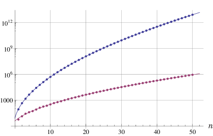
Figure 1. Exact values of $A_{n}$ (3.9) and values of the asymptotic formula (4.22) are given by blue dots and blue line, respectively. We have also plotted exact absolute values $|A_{n}^{\circ}|$ (3.14) together with their asymptotic values (4.28) in red.

In the tables we present more detailed results. We have numerically computed the exact asymptotic series (4.21) of $A_{n}$ by truncating the infinite sum $\sum_{c=1}^{\infty}$ by a finite number of terms. For comparison we also list the exact values of $A_{n}$;

$$\begin{array}[]{r||r|rrr}n&\mbox{exact}&\mbox{leading};\,\eqref{asymptotics_A}&\text{sum of $5$ terms}&\text{$20$ terms}\\ \hline\cr\hline\cr 2&462&453.018&462.026&462.427\\ 5&11592&11662.495&11594.141&11592.421\\ 20&126894174&126889894.140&126894174.078&126894173.718\\ 30&9104078592&9104043456.138&9104078600.515&9104078592.403\\ 40&342322413552&342322217629.135&342322413549.736&342322413551.574\\ 45&1778826191324&1778826619936.736&1778826191295.658&1778826191322.367\end{array}$$

For the case of $A_{n}^{\circ}$, we also present their exact values and values given by the truncation of the asymptotic expansion (4.27)

$$\begin{array}[]{r||r|rrr}n&\mbox{exact}&\mbox{leading};\,\eqref{asymptotics_AC}&\text{sum of $5$ terms}&\text{$10$ terms}\\ \hline\cr\hline\cr 5&-56&-61.111&-56.544&-56.336\\ 20&4510&4486.206&4511.303&4509.981\\ 21&-5544&-5598.785&-5543.374&-5543.584\\ 40&195888&195787.459&195888.432&195887.820\\ 60&3772468&3772123.173&3772465.128&3772468.117\\ 100&438370422&438366833.884&438370424.848&438370421.862\end{array}$$

One sees that numerical results support the convergence of the series (4.16) the validity of our asymptotic formulae (4.21) and (4.27).

For its direct verification, we have numerically computed (4.19) to obtain

$$\mathrm{i}\sqrt{\Im\tau}\,\overline{\frac{\partial}{\partial\overline{\tau}}P_{\frac{3}{4}}(8\,\tau)}=23.851\,{q}-72.0946\,{q}^{9}+0.320386\,{q}^{17}+119.083\,{q}^{25}\\ +0.295543\,{q}^{33}+0.152477\,{q}^{41}-166.728\,{q}^{49}-0.587912\,{q}^{57}\\ -0.0773375\,{q}^{65}-0.652751\,{q}^{73}+213.397\,{q}^{81}-0.217745\,{q}^{89}+\cdots.$$

Here we have truncated the sum over $c$ after the first $800$ terms. Though the convergence is slower than before, this agrees with (4.20).

5. Chern–Simons Theory

A key in our analysis is to complete the massless superconformal character $\mu(z;\tau)$ by adding the non-holomorphic partner $R(\tau)$ (2.9) so that the sum has a nice modular property. Here we would like to point out that $R(\tau)$ has its own meaning as a topological quantum invariant related to a simple singularity.

The Witten invariant of 3-manifold $M$ [45] is defined by the Chern–Simons path integral

$$Z_{k}(M)=\int\mathrm{e}^{2\,\pi\,\mathrm{i}\,k\,\operatorname{CS}(A)}\mathcal{D}A,$$ (5.1)

where the coupling constant $k\in\mathbb{Z}$ denotes the level, and $A$ is a $G$-gauge connection on the trivial bundle over $M$. The Chern–Simons action $\operatorname{CS}(A)$ with gauge group $G$ is

$$\operatorname{CS}(A)=\frac{1}{8\,\pi^{2}}\int\limits_{M}\operatorname{Tr}\left(A\wedge\mathrm{d}A+\frac{2}{3}\,A\wedge A\wedge A\right).$$

See Ref. 42 for mathematically rigorous definition of this quantum invariant (Witten–Reshetikhin–Turaev invariant) in terms of the quantum invariants of links to be surgered. When $M$ is the Poincaré homology sphere, it was shown that the Witten invariant $Z_{k}(M)$ with gauge group $SU(2)$ can be regarded as a limiting value of the Eichler integral of a weight-$3/2$ modular form [31]. This correspondence has been checked for other Seifert manifolds [26, 27].

Let $M$ be the Seifert manifold $M(2,2,2)$ [35], which is a spherical neighborhood around the isolated singularity of type-$D_{4}$;

$$M=\left\{x^{2}\,y+y^{3}+z^{2}=0\right\}\cap S^{5},$$

where $S^{5}$ denotes a sufficiently small $5$-sphere around the origin. It was shown [27] that the Witten invariant $Z_{k}(M)$ with SU($2$) gauge group is given by (see also Refs. 28, 25)

$$Z_{k}(M)=\frac{1}{2\,\mathrm{i}}\,\sqrt{\frac{2}{k+2}}\,\mathrm{e}^{-\frac{1}{k+2}\,\pi\,\mathrm{i}}\,\left[1-\mathrm{e}^{-\frac{1}{4(k+2)}\pi\mathrm{i}}\,R\left(-\frac{1}{k+2}\right)\right].$$ (5.2)

Here $R(\tau)$ is the period integral of the third power of the Dedekind $\eta$-function (2.12), and we have a limiting value in $\tau\to-\frac{1}{k+2}$. It was shown that the topological invariants, such as the Chern–Simons invariant, the Reidemeister torsion, and the Ohtsuki invariant, of $M$ are given by the asymptotic expansion of $Z_{k}(M)$ in $k\to\infty$.

It should also be noted that the non-holomorphic partner of the massless character $R(\tau)$ is related to the knot invariant for the torus link $T_{2,4}$ [24]

$$\left\langle T_{2,4}\right\rangle_{N}=N\,\mathrm{e}^{-\frac{1}{4N}\,\pi\,\mathrm{i}}\,R\left(-\frac{1}{N}\right).$$ (5.3)

Here $\left\langle L\right\rangle_{N}$ denotes a specific value of the $N$-colored Jones polynomial for link $L$ at $q=\mathrm{e}^{2\pi\mathrm{i}/N}$: this quantity receives renewed interests from the viewpoint of the volume conjecture raised by Kashaev [29], and H. Murakami and J. Murakami [37].

6. Concluding Remarks

As an application of our previous result [12] that the coefficients of massive characters of the elliptic genera are the holomorphic part of harmonic Maass form, we have obtained their Rademacher-type expansion by computing the Fourier coefficients of the Poincaré–Maass series.

We note that in the elliptic genus the right-moving sector is fixed to Ramond ground state and thus the non-BPS states in the left-moving sector are actually the overall half-BPS states (BPS (non-BPS) in the right (left) moving sector). It is known that asymptotic increase of the number of half-BPS states is related to the entropy of supersymmetric systems. In fact the multiplicity factor $A_{n}$ behaves like an exponential (4.23) and we may identity

$$S=2\,\pi\,\sqrt{{1\over 2}\,n}$$ (6.1)

as the entropy of K3 surface.

Our methods are applicable to higher level superconformal algebras and higher-dimensional hyperKähler manifolds. In general hyperKähler manifolds with complex $2k$-dimensions we find an entropy  [13]

$$S=2\,\pi\,\sqrt{{k^{2}\over k+1}\,n}.$$ (6.2)

If we consider the case of symmetric product of K3 surfaces $K3^{[k]}$, the above entropy reproduces the black hole entropy of string theory compactified on K3 surface at large $k$.

Appendix A Jacobi Theta Functions

The Jacobi theta functions are defined by

$$\theta_{11}(z;\tau) =\sum_{n\in\mathbb{Z}}q^{\frac{1}{2}\left(n+\frac{1}{2}\right)^{2}}\,\mathrm{e}^{2\pi\mathrm{i}\left(n+\frac{1}{2}\right)\,\left(z+\frac{1}{2}\right)}=\theta_{1}(z;\tau),$$

$$\theta_{10}(z;\tau) =\sum_{n\in\mathbb{Z}}q^{\frac{1}{2}\left(n+\frac{1}{2}\right)^{2}}\,\mathrm{e}^{2\pi\mathrm{i}\left(n+\frac{1}{2}\right)z}=\theta_{2}(z;\tau),$$

$$\theta_{00}(z;\tau) =\sum_{n\in\mathbb{Z}}q^{\frac{1}{2}n^{2}}\,\mathrm{e}^{2\pi\mathrm{i}nz}=\theta_{3}(z;\tau),$$

$$\theta_{01}(z;\tau) =\sum_{n\in\mathbb{Z}}q^{\frac{1}{2}n^{2}}\,\mathrm{e}^{2\pi\mathrm{i}n\left(z+\frac{1}{2}\right)}=\theta_{4}(z;\tau),$$

where we have also shown the relation to the conventional notations.

References

• [1] G. E. Andrews, On the theorems of Watson and Dragonette for Ramanujan’s mock theta functions, Amer. J. Math. 88, 454–490 (1966).
• [2] ———, The Theory of Partitions, Addison-Wesley, London, 1976.
• [3] ———, Mock theta functions, in L. Ehrenpreis and R. C. Gunning, eds., Theta Functions — Bowdoin 1987, vol. 49 (part 2) of Proc. Symp. Pure Math., pp. 283–298, Amer. Math. Soc., Providence, 1989.
• [4] K. Bringmann and K. Ono, The $f(q)$ mock theta function conjecture and partition ranks, Invent. Math. 165, 243–266 (2006).
• [5] ———, Coefficients of harmonic Maass forms, preprint (2008).
• [6] J. H. Bruinier, Borcherds Products on $O(2,\ell)$ and Chern Classes of Heegner Divisors, vol. 1780 of Lecture Notes in Mathematics, Springer, Berlin, 2002.
• [7] J. H. Bruinier and J. Funke, On two geometric theta lifts, Duke Math. J. 125, 45–90 (2004).
• [8] H. Cohen and J. Oesterlé, Dimensions des espaces de formes modulaires, in J.-P. Serre and D. Zagier, eds., Modular Functions of One Variable VI, vol. 627 of Lecture Notes in Mathematics, pp. 69–78, Springer, Berlin, 1977.
• [9] R. Dijkgraaf, J. Maldacena, G. Moore, and E. Verlinde, A black hole Farey tail, hep-th/0005003v3 (2007).
• [10] L. Dragonette, Some asymptotic formulae for the mock theta series of Ramanujan, Trans. Amer. Math. Soc. 72, 474–500 (1952).
• [11] F. J. Dyson, Some guesses in the theory of partitions, Eureka (Cambridge) 8, 10–15 (1944).
• [12] T. Eguchi and K. Hikami, Superconformal algebras and mock theta functions, J. Phys. A: Math. Theor. 42, 304010 (2009), 23 pages.
• [13] ———, preprint in preparation.
• [14] T. Eguchi, H. Ooguri, A. Taormina, and S.-K. Yang, Superconformal algebras and string compactification on manifolds with SU($n$) holonomy, Nucl. Phys. B 315, 193–221 (1989).
• [15] T. Eguchi, Y. Sugawara, and A. Taormina, Liouville field, modular forms and elliptic genera, JHEP 2007, 119 (2007), 21 pages.
• [16] ———, Modular forms and elliptic genera for ALE spaces, arXiv:0803.0377 (2008).
• [17] T. Eguchi and A. Taormina, Unitary representations of the $N=4$ superconformal algebra, Phys. Lett. B 196, 75–81 (1986).
• [18] ———, Character formulas for the $N=4$ superconformal algebra, Phys. Lett. B 200, 315–322 (1988).
• [19] ———, On the unitary representations of $N=2$ and $N=4$ superconformal algebras, Phys. Lett. B 210, 125–132 (1988).
• [20] M. Eichler and D. Zagier, The Theory of Jacobi Forms, vol. 55 of Progress in Mathematics, Birkhäuser, Boston, 1985.
• [21] B. Gordon and R. J. McIntosh, A survey of classical mock theta functions, preprint (2009).
• [22] G. H. Hardy and S. Ramanujan, Asymptotic formulæ in combinatory analysis, Proc. London Math. Soc. 2, 75–115 (1918).
• [23] D. A. Hejhal, The Selberg Trace Formula for PSL($2,\mathbb{R}$) Vol. 2, vol. 1001 of Lecture Notes in Mathematics, Springer, Berlin, 1983.
• [24] K. Hikami, Quantum invariant for torus link and modular forms, Commun. Math. Phys. 246, 403–426 (2004).
• [25] ———, Mock (false) theta functions as quantum invariants, Regular & Chaotic Dyn. 10, 509–530 (2005).
• [26] ———, On the quantum invariant for the Brieskorn homology spheres, Int. J. Math. 16, 661–685 (2005).
• [27] ———, On the quantum invariant for the spherical Seifert manifold, Commun. Math. Phys. 268, 285–319 (2006).
• [28] ———, Transformation formula of the “2nd” order mock theta function, Lett. Math. Phys. 75, 93–98 (2006).
• [29] R. M. Kashaev, The hyperbolic volume of knots from quantum dilogarithm, Lett. Math. Phys. 39, 269–275 (1997).
• [30] T. Kawai, Y. Yamada, and S.-K. Yang, Elliptic genera and $N=2$ superconformal field theory, Nucl. Phys. B 414, 191–212 (1994).
• [31] R. Lawrence and D. Zagier, Modular forms and quantum invariants of 3-manifolds, Asian J. Math. 3, 93–107 (1999).
• [32] A. Malmendier and K. Ono, SO(3)-Donaldson invariants of $\mathbb{C}\mathrm{P}^{2}$ and mock theta functions, arXiv:0808.1442 (2008).
• [33] A. Maloney and E. Witten, Quantum gravity partition function in three dimensions, arXiv:0712.0155 (2007).
• [34] J. Manschot and G. W. Moore, A modern Farey tail, arXiv:0712.0573 (2007).
• [35] J. Milnor, On the 3-dimensional Brieskorn manifolds $M(p,q,r)$, in L. P. Neuwirth, ed., Knots, Groups, and 3-Manifolds, pp. 175–225, Princeton Univ. Press, 1975, papers Dedicated to the Memory of R. H. Fox.
• [36] G. Moore, Strings and arithmetic, in P. Cartier, B. Julia, and P. Moussa, eds., Frontiers in Number Theory, Physics and Geometry II, pp. 303–359, Springer, Berlin, 2006.
• [37] H. Murakami and J. Murakami, The colored Jones polynomials and the simplicial volume of a knot, Acta. Math. 186, 85–104 (2001).
• [38] K. Ono, The Web of Modularity: Arithmetic of the Coefficients of Modular Forms and $q$-series, no. 102 in CBMS Regional Conference Series in Math., Amer. Math. Soc., Providence, 2004.
• [39] ———, Unearthing the visions of a master: harmonic Maass forms and number theory, Proceedings of the 2008 Harvard-MIT Current Developments in Mathematics Conference, Intl. Press, Boston, in press.
• [40] D. N. Page, A physical picture of the K3 gravitational instanton, Phys. Lett. B 80, 55–57 (1978).
• [41] H. Rademacher, Topics in Analytic Number Theory, vol. 169 of Die Grundlehren der mathematischen Wissenschaften, Springer, New York, 1973.
• [42] N. Yu. Reshetikhin and V. G. Turaev, Invariants of 3-manifolds via link polynomials and quantum groups, Invent. Math. 103, 547–597 (1991).
• [43] E. T. Whittaker and G. N. Watson, A Course of Modern Analysis, Cambridge Univ. Press, Cambridge, 1927, 4th ed.
• [44] E. Witten, Elliptic genera and quantum field theory, Commun. Math. Phys. 109, 525–536 (1987).
• [45] ———, Quantum field theory and the Jones polynomial, Commun. Math. Phys. 121, 351–399 (1989).
• [46] D. Zagier, Ramanujan’s mock theta functions and their applications [d’après Zwegers and Bringmann–Ono], Séminaire Bourbaki 986 (2006–2007).
• [47] S. P. Zwegers, Mock Theta Functions, Ph.D. thesis, Universiteit Utrecht (2002).