Quantum switch for single-photon transport in a coupled superconducting transmission line resonator array

Abstract

We propose and study an approach to realize quantum switch for single-photon transport in a coupled superconducting transmission line resonator (TLR) array with one controllable hopping interaction. We find that the single-photon with arbitrary wavevector can transport in a controllable way in this system. We also study how to realize controllable hopping interaction between two TLRs via a Cooper pair box (CPB). When the frequency of the CPB is largely detuned from those of the two TLRs, the variables of the CPB can be adiabatically eliminated and thus a controllable interaction between two TLRs can be obtained.

Coupled cavity arrays (CCAs) CCAreview have recently attracted considerable attentions of both theorists and experimentalists. The CCAs have been proposed to implement quantum simulators for many-body physics, such as discovering new matter phases of photons HBP06 ; GTCH06 ; RF07 and providing a new platform to study spin systems ASB07 ; HBP07a . The CCAs are also suggested to manipulate photons for optical quantum information processing HLSS08 ; BAB07 ; ASYE07 . Moreover, photon transport in the CCAs has been investigated ZLS07 ; ZGLSN08 ; HZSS07 ; ZGSS08 ; GIZS08 . There are several possible ways to construct the CCAs, for example: (i) coupled defect cavities in photonic crystals Vuckovic ; (ii) coupled toroidal microresonators AKSV03 ; and (iii) coupled superconducting transmission line resonators (TLRs) ZGLSN08 ; HZSS07 .

In CCAs, there have been many proposals to realize quantum switch sun ; Switch , which is used to control single-photon transport ZGLSN08 ; Lukin-np ; Fanpaper1 ; Fanpaper2 . For example, the reflection and transmission of photons in a coupled resonator waveguide can be controlled by a tunable two-level quantum system ZGLSN08 ; Switch , acting as a controller.

Here, we study another approach to control the single-photon transport in a CCA, which consists of a chain of TLRs Wal04 ; Blais04 . In our proposal, the controllable transport is realized by a tunable coupling. As we know, how to control coupling between two solid devices is a major challenge in scalable quantum computing circuits you ; you1 ; liu ; miro ; yingdan ; yingdan2 ; Hu . To obtain a tunable coupling, we propose that a Cooper pair box (CPB) acts as a coupler. When the frequency of the coupler is largely detuned from those of the two resonators, the variables of the coupler can be adiabatically eliminated and thus a controllable interaction can be induced. Compared with previous approach ZGLSN08 , this approach has following advantage: dynamical variables of the coupler are adiabatically eliminated, therefore the coupler is a passive controlling element, which makes robust to prevent from the environment of the coupler.

As shown in Fig. 1, one-dimensional CCA is a chain of $N$ cavities, each is only coupled to its nearest-neighbor ones, Fig. 1(a) and (b) are the site lattice model and the schematic diagram of coupled TLR array, respectively. The TLRs are assumed to have the same frequency. We also assume that the coupling strength between two nearest-neighbor TLRs is the same, except one between the $l$-th and $(l+1)$-th TLRs. The Hamiltonian of the system is

$$H = \omega\sum_{n}a_{n}^{{\dagger}}a_{n}-t\sum_{n}(a_{n}^{{\dagger}}a_{n+1}+a_{n+1}^{{\dagger}}a_{n})$$ (1)

$$-\lambda t(a_{l}^{{\dagger}}a_{l+1}+a_{l+1}^{{\dagger}}a_{l}),$$

hereafter we take $\hbar=1$. Here, we assume that all TLRs have the same frequency $\omega$. $a^{{\dagger}}_{n}$ and $a_{n}$ are the creation and annihilation operators of $n$-th TLR; $t$ is the coupling strength between the $n$-th ($n\neq l$) and $(n+1)$-th TLRs; $\lambda=(t^{\prime}-t)/t$ is introduced to denote the relation between $t$ and $t^{\prime}$, where $t^{\prime}$ is the coupling strength between the $l$-th and $(l+1)$-th TLRs. Obviously, $-1<\lambda<0$ corresponds to $0<t^{\prime}<t$, while $\lambda\geq 0$ implies $t^{\prime}\geq t$. Below we will first study how to control the single-photon transport by changing coupling strength $t^{\prime}$, and then answer question how to realize controllable coupling $t^{\prime}$.

In the case of $t^{\prime}=t$, the Hamiltonian in Eq. (1) is reduced to the usual bosonic tight binding model $H_{\textrm{btb}}=\omega\sum_{n}a_{n}^{{\dagger}}a_{n}-t\sum_{n}(a_{n}^{{\dagger}}a_{n+1}+a_{n+1}^{{\dagger}}a_{n})$ as shown in Ref. Data , which describes an $N$-site lattice model with nearest-neighbor coupling. It is well known that, under the periodic boundary condition, the bosonic tight binding Hamiltonian can be diagonalized as $H_{\textrm{btb}}=\sum_{k}\Omega_{k}a_{k}^{{\dagger}}a_{k}$ by using the Fourier transformation $a_{k}=\sum_{n}\exp(iknd_{0})a_{n}/\sqrt{N}$, where $d_{0}$ is the site distance. Below, $d_{0}$ is taken as units. We choose the wavevectors $k=2\pi m/N$ within the first Brillouin zone, i.e., $-N/2<m\leq N/2$. The corresponding dispersion relation is $\Omega_{k}=\omega-2t\cos k$, which is an energy band structure. For $t>0$, the wavevectors $k=\pm\pi/2$ correspond to the energy band center, while the wavevectors $k=0$ and $k=\pm\pi$ correspond to the bottom and top of the energy band, respectively.

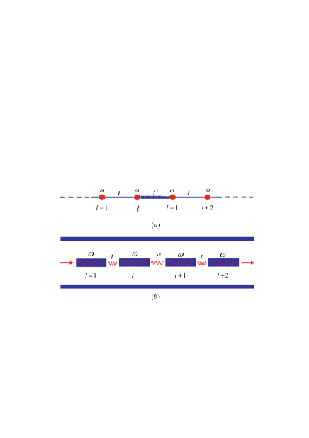
Figure 1: (Color online) Schematic configuration for controllable transport of single photon: (a) one-dimensional site lattice model for the coupled cavity array; (b) schematic diagram of coupled superconducting transmission line resonator array.

Let us now define a total excitation number operator $\hat{N}=\sum_{n}a_{n}^{{\dagger}}a_{n}$. It is straightforward to show that $\hat{N}$ commutes with the model Hamiltonian (1), i.e., $[\hat{N},H]=0$, which implies that the total excitation number $\hat{N}$ is a conserved observable. We now restrict our discussion to the single excitation subspace since we only consider the single-photon transport. In this case, a general state can be written as $|\Omega\rangle=\sum_{n}A_{n}|1_{n}\rangle$, where we have introduced the basis state $|1_{n}\rangle=|0\rangle\otimes...\otimes|1\rangle_{n}\otimes...\otimes|0\rangle$, which represents the state that the $n$-th TLR has one photon while other TLRs have no photon. $A_{n}$ is the probability amplitude of the state $|1_{n}\rangle$. Using the discrete scattering method proposed in Ref. ZGLSN08 and according to the eigenequation $H|\Omega\rangle=\Omega|\Omega\rangle$, we have

$$-t(A_{n+1}+A_{n-1}) =(\Omega-\omega)A_{n},\hskip 8.5359ptn\neq\{l,l+1\},$$ (2a)

$$-t^{\prime}A_{l+1}-tA_{l-1} =(\Omega-\omega)A_{l},$$ (2b)

$$-A_{l+2}-t^{\prime}A_{l} =(\Omega-\omega)A_{l+1}.$$ (2c)

For the coherent transport of a single-photon with the energy $\Omega=\omega-2t\cos k$, we can assume the following forms for the probability amplitudes

$$A_{n} =e^{ikn}+re^{-ikn},\hskip 8.5359pt(n\leq l),$$ (3a)

$$A_{n} =se^{ikn},\hskip 8.5359pt(n\geq l+1).$$ (3b)

Here $r$ and $s$ are the reflection and transmission amplitudes, respectively. Obviously, Eqs. (3a) and (3b) are the solutions of Eq. (2a). Substituting Eqs. (3a) and (3b) into Eqs. (2b) and (2c), we can obtain the transmission coefficient

$$T(\lambda,k)=\frac{4(\lambda+1)^{2}\sin^{2}k}{\lambda^{2}(\lambda+2)^{2}+4(\lambda+1)^{2}\sin^{2}k},$$ (4)

and the reflection coefficient $R(\lambda,k)=|s|^{2}=1-T(\lambda,k)$. Eq. (4) shows that the reflection and transmission coefficients $R(\lambda,k)$ and $T(\lambda,k)$ are function of the parameter $\lambda$ and the wavevector $k$ of the incident photon, and they are independent of other variables, e.g., the site position parameter $l$, the cavity frequency $\omega$, and the coupling constant $t$.

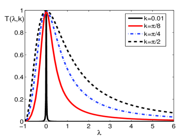
Figure 2: (Color online) The transmission coefficient $T$ versus the parameter $\lambda$ for different wavevectors k=0.01, $\pi/8$, $\pi/4$, and $\pi/2$ is plotted.

Equation (4) shows two symmetry relations $T(\lambda,k)=T(\lambda,-k)$ and $T(\lambda,\pi/2-k)=T(\lambda,\pi/2+k)$. Therefore we need only to analyze the transmission coefficient within the region $0\leq k\leq\pi/2$. In this region, there are four special cases: (1) $T(\lambda\neq 0,0)=0$, when the wavevector $k=0$, for $\lambda\neq 0$, the input single photon is reflected completely; (2) $T(\lambda=-1,k)=0$, when $\lambda=-1$, the coupling between the $l$-th and $(l+1)$-th cavities is switched off, so for any value of the wavevector $k$, the transmission coefficient is zero; (3) $T(\lambda\rightarrow\infty,k)=0$, when $\lambda\rightarrow\infty$, namely, $t^{\prime}\gg t$, the transmission coefficient is zero for any $k$. Physically, when $t^{\prime}\gg t$, the Hamiltonian (1) is approximated to $H(t^{\prime}\gg t)\approx-t^{\prime}(a^{\dagger}_{l}a_{l+1}+a^{\dagger}_{l+1}a_{l})$. The input photon will stay in the $l$-th and $(l+1)$-th cavities once it arrives the $l$-th cavity; (4) $T(\lambda=0,k)=1$, $\lambda=0$ implies $t^{\prime}=t$, the present model reduces to the usual bosonic tight binding model, so the photon with any wavevector can be perfectly transported.

To observe the effect on the transmission coefficient $T$ for general wavevector $k$ and parameter $\lambda$, in Fig. 2, the transmission coefficient $T$ is plotted as a function of the parameter $\lambda$ for wavevectors $k=0.01$, $\pi/8$, $\pi/4$, and $\pi/2$. Fig. 2 indicates that there are two regions, $-1\leq\lambda\leq 0$ and $0\leq\lambda$, in which controllable transport of single photon can be achieved. The transmission coefficient $T$ can be tuned from $0$ to $1$ by changing the coupling strength $t^{\prime}$, namely $\lambda$. When $t^{\prime}=0$, the transmission coefficient $T=0$. With the increase of the coupling strength $t^{\prime}\rightarrow t$, the transmission coefficient $T$ gradually approaches to 1. For $t^{\prime}\geq t$, the transmission coefficient $T$ approaches to $0$ with the increase of the coupling $t^{\prime}\rightarrow\infty$. In this region, the larger wavevector $k$ corresponds to the larger parameter range of $\lambda$. In both regions, the controllable transport of single-photon with arbitrary wavevector $k$ can be realized. Therefore, our approach for single-photon transport can cover complete bandwidth.

Let us now focus the problem on how to realize controllable coupling between two TLRs Switch ; miro . The system we considered is shown in Fig. 3. Two TLRs are coupled to a CPB through capacitors $C_{l}$ and $C_{r}$, respectively. We assume that the two TLRs are identical, that is, they have the same length $d$ and capacitance $C_{0}$ (inductance $L_{0}$) per unit length. We consider only single-modes of the two TLRs in near resonant with the CPB. The free Hamiltonian of the two TLRs is

$$H_{\textrm{TLR}}=\omega a_{l}^{{\dagger}}a_{l}+\omega a_{r}^{{\dagger}}a_{r},$$ (5)

where $a^{\dagger}_{l}$ ($a^{\dagger}_{r}$) and $a_{l}$ ($a_{r}$) are the creation and annihilation operators of the resonant modes with frequency $\omega$ for the left (right) TLR, respectively.

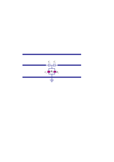
Figure 3: (Color online) Schematic diagram for two TLRs (the left and the right ones), which are coupled to a CPB through two capacitors $C_{l}$ and $C_{r}$, respectively. The CPB is biased by a magnetic flux $\Phi_{x}$

The CPB is a superconducting loop interrupted by two identical Josephson junctions with the capacitance $C_{J}$ and the Josephson energy $E^{(0)}_{J}$. To obtain a tunable Josephson coupling energy, an external magnetic flux $\Phi_{x}$ is applied through the superconducting loop. The Hamiltonian of the CPB is

$$H^{\prime}_{\textrm{CPB}} = E_{C}\,n^{2}-E_{J}(\Phi_{x})\cos\varphi,$$ (6)

where $n$ is the number operator of Cooper-pair charges on the island connected to the CPB, and $\varphi$ is the superconducting phase difference across the Josephson junction. The charging energy $E_{C}$ and effective Josephson energy $E_{J}(\Phi_{x})$ of the CPB are $E_{C}=2e^{2}/(C_{l}+C_{r}+2C_{J})$ and $E_{J}(\Phi_{x})=2E^{(0)}_{J}\cos(\pi\Phi_{x}/\Phi_{0})$, respectively. Here, we assume that the charging energy and the effective Josephson energy satisfy the condition $E_{J}(\Phi_{x})\gg E_{C}$. Under this condition, the spectrum of the lowest energy levels of the CPB can be described approximately by a harmonic oscillator yingdan2 . That is, we expand $E_{J}(\Phi_{x})\cos\varphi$ around $\varphi=0$ up to $\mathcal{O}(\varphi^{2})$, and then Eq. (6) becomes

$$H_{\textrm{CPB}}=\omega_{b}b^{{\dagger}}b,\hskip 8.5359pt\omega_{b}=\sqrt{2E_{C}E_{J}(\Phi_{x})}.$$ (7)

The annihilation and creation operators $b$ and $b^{{\dagger}}$ in Eq. (7) are defined in terms of $\varphi=\sqrt[4]{E_{C}/(2E_{J}(\Phi_{x}))}(b+b^{{\dagger}})$ and $n=-i\sqrt[4]{E_{J}(\Phi_{x})/(8E_{C})}(b-b^{{\dagger}})$.

We assume that the linear dimension of the CPB is much smaller than wavelengths of the TLRs, and choose the position of the CPB at the origin of the axis. Then the quantized voltages at the left and right TLRs are

$$V_{j}(0)=-i\sqrt{\frac{\omega}{dC_{0}}}(a_{j}-a^{{\dagger}}_{j}),\hskip 8.5359ptj=l,r.$$ (8)

According to circuit theory, we know that the voltage at the island is $\Phi_{0}\dot{\varphi}/(2\pi)$. Therefore, the Coulomb interaction induced by the two capacitors $C_{l}$ and $C_{r}$ is

$$H_{I}=\sum_{j=l,r}\frac{C_{j}}{2}\left(V_{j}(0)-\frac{\Phi_{0}}{2\pi}\dot{\varphi}\right)^{2}.$$ (9)

In fact, capacitors $C_{l}$ and $C_{r}$ induce a direct Coulomb interaction between the two TLRs with the strength $\propto C_{l}C_{r}$. However, this direct interaction is much smaller than the interaction between the two TLRs and the CPB given by Eq. (9) with strengths $\propto C_{\Sigma l}C_{r}$ and $\propto C_{\Sigma r}C_{l}$ under the condition $\{C_{\Sigma l},C_{\Sigma r}\}>>\{C_{l},C_{r}\}$, where $C_{\Sigma l}=C_{0}d/2+C_{l}$ and $C_{\Sigma r}=C_{0}d/2+C_{r}$ are the sum capacitors connected to the left and right TLRs, respectively Li . For instance, using current experimental parameters Frunzio $C_{0}d/2\sim 1.6$ pF and $C_{l}=C_{r}=6$ fF, we find that the interaction between the TLRs and the CPB is larger than the direct interaction between two TLRs by three orders of magnitude.

Using Eqs. (5-9), the total Hamiltonian of the system described in Fig. 3 is

$$H = \omega_{l}a_{l}^{{\dagger}}a_{l}+\omega_{r}a_{r}^{{\dagger}}a_{r}+\omega^{\prime}_{b}b^{{\dagger}}b$$ (10)

$$+g_{l}(a_{l}b^{{\dagger}}+ba_{l}^{{\dagger}})+g_{r}(a_{r}b^{{\dagger}}+ba_{r}^{{\dagger}}),$$

where we have introduced the renormalized frequencies

$$\omega_{j} =\omega\left(1+\frac{C_{j}}{dC_{0}}\right),\hskip 28.45274ptj=l,r,$$ (11a)

$$\omega^{\prime}_{b} =\omega_{b}+(C_{l}+C_{r})\omega_{b}^{2}\left(\frac{\Phi_{0}}{2\pi}\right)^{2}\left(\frac{E_{C}}{2E_{J}(\Phi_{x})}\right)^{\frac{1}{2}},$$ (11b)

and the coupling strengths

$$g_{j} =-C_{j}\omega_{b}\frac{\Phi_{0}}{2\pi}\sqrt{\frac{\omega}{dC_{0}}}\left(\frac{E_{C}}{2E_{J}(\Phi_{x})}\right)^{\frac{1}{4}},\hskip 8.5359ptj=l,r.$$ (12)

It should be noted that we have made the rotation wave approximation when Eq. (10) is derived.

Equation (10) describes that two TLRs are coupled to the CPB, which serves as a coupler. To obtain controllable coupling between the two TLRs, we restrict the system in the large detuning regime, where the frequency differences between the two TLRs and the CPB are much larger than their coupling constants, i.e., $\Delta_{l}\gg g_{l}$ and $\Delta_{r}\gg g_{r}$. Here, $\Delta_{j}=\omega^{\prime}_{b}-\omega_{j}$ for $j=l,r$ are the dutuning between the frequencies of the TLRs and that of the CPB. By adiabatically eliminating the degree of freedom of the CPB, we obtain an effective interaction between the two TLRs. That is, we perform a unitary transform $U=\exp[g_{l}(a_{l}b^{{\dagger}}-ba_{l}^{{\dagger}})/\Delta_{l}+g_{r}(a_{r}b^{{\dagger}}-ba_{r}^{{\dagger}})/\Delta_{r}]$ for the Hamiltonian in Eq. (10) and use the Hausdorff expansion up to the first order in the small parameter $g_{j}/\Delta_{j}$ with $j=l,\,r$, then we obtain an effective Hamiltonian

$$H_{\textrm{eff}} = \omega^{\prime}_{l}a_{l}^{{\dagger}}a_{l}+\omega^{\prime}_{r}a_{r}^{{\dagger}}a_{r}+g(a_{r}a_{l}^{{\dagger}}+a_{l}a_{r}^{{\dagger}}),$$ (13)

where we have defined the Stark-shifted frequencies $\omega^{\prime}_{j}=\omega_{j}+g^{2}_{j}/\Delta_{j}$ for $j=l,r$, and the effective coupling strength

$$g=\frac{g_{l}g_{r}(\Delta_{l}+\Delta_{r})}{2\Delta_{l}\Delta_{r}}.$$ (14)

Note that the effective Hamiltonian of the CPB $H_{\textrm{CPB}}=\omega^{\prime\prime}_{b}b^{{\dagger}}b$ with $\omega^{\prime\prime}_{b}=\omega^{\prime}_{b}-g^{2}_{l}/\Delta_{l}-g^{2}_{r}/\Delta_{r}$ has been neglected in Eq. (13). It is obvious that the Hamiltonian (13) describes an effective interaction between the two TLRs. According to Eqs. (7) and (11b), the frequency of the CPB can be tuned by the external magnetic flux $\Phi_{x}$. Correspondingly, the detunings $\Delta_{l}$ and $\Delta_{r}$ between the TLRs and the CPB can be tuned, thus the coupling constant $g$ can be tuned. When the detunings are very larger than the coupling constants between the TLRs and the CPB, the effective coupling constant $g$ between the two TLRs are negligibly small, and then the interaction between the two TLRs is switched off. For example, if we assume that the two transmission line resonators are identical, i.e., $\Delta_{l}=\Delta_{r}=\Delta$ and $g_{l}=g_{r}=g^{\prime}$, and we take the parameters Frunzio : $\omega=2\pi\times 3$ GHz, $C_{l}=C_{r}=6$ fF, $C_{0}d=1.6$ pF, $E_{C}=2\pi\times 0.35$ GHz, $E^{(0)}_{J}\sim 10^{3}E_{C}$, then we calculate $g\approx 1.1\sim 23$ MHz corresponding to $\cos(\pi\Phi_{x}/\Phi_{0})\approx 0.02\sim 1$. In this region, the conditions $E_{J}(\Phi_{x})\gg E_{C}$ and $\Delta\gg g^{\prime}$ are satisfied.

In conclusion, we have studied a quantum switch for single-photon transport in a coupled TLR array with one controllable hopping interaction. We have found that the controllable single-photon transport, for an arbitrary wavevector of photons, in the coupled TLR array can be realized by tuning one of the coupling constants. How to realize the controllable coupling between two TLRs is also studied. We have proposed that a CPB serves as a coupler to connect the two TLRs. In the regime of $E_{J}(\Phi_{x})\gg E_{C}$, the CPB is approximately described as a harmonic oscillator. Under the large detuning condition, we have obtained an effective interaction between the TLRs by adiabatically eliminating the variables of the CPB. This induced effective coupling can be controlled by the external magnetic flux $\Phi_{x}$ through the CPB.

This work is supported by the NSFC with Grant Nos. 10474104, 60433050, 10704023, and 10775048; NFRPC Nos. 2006CB921205, 2005CB724508, and 2007CB925204.

References

- (1) M. J. Hartmann, F. G. S. L. Brando, and M. B. Plenio, Laser and Photon Rev. 2, No. 6, 527 (2008) and references therein.
- (2) M. J. Hartmann, F. G. S. L. Brando, and M. B. Plenio, Nat. Phys. 2, 849 (2006).
- (3) A. D. Greentree, C. Tahan, J. H. Cole, and L. C. L. Hollenberg, Nat. Phys. 2, 856 (2006).
- (4) D. Rossini and R. Fazio, Phys. Rev. Lett. 99, 186401 (2007).
- (5) D. G. Angelakis, M. F. Santos, and S. Bose, Phys. Rev. A 76, R031805 (2007).
- (6) M. J. Hartmann, F. G. S. L. Brando, and M. B. Plenio, Phys. Rev. Lett. 99, 160501 (2007).
- (7) M. X. Huo, Y. Li, Z. Song, and C. P. Sun, Phys. Rev. A 77, 022103 (2008).
- (8) S. Bose, D. G. Angelakis, and D. Burgarth, J. Mod. Opt. 54, 2307 (2007).
- (9) D. G. Angelakis, M. F. Santos, V. Yannopapas, and A. Ekert, Phys. Lett. A. 362, 377 (2007).
- (10) L. Zhou, J. Lu, and C. P. Sun, Phys. Rev. A 76, 012313 (2007).
- (11) L. Zhou, Z. R. Gong, Y. X. Liu, C. P. Sun, and F. Nori, Phys. Rev. Lett. 101, 100501 (2008).
- (12) F. M. Hu, L. Zhou, T. Shi, and C. P. Sun, Phys. Rev. A 76, 013819 (2007).
- (13) L. Zhou, Y. B. Gao, Z. Song, and C. P. Sun, Phys. Rev. A 77, 013831 (2008).
- (14) Z. R. Gong, H. Ian, L. Zhou, and C. P. Sun, Phys. Rev. A 78, 053806 (2008).
- (15) H. Altug and J. Vuckovic, Appl. Phys. Lett. 84, 161 (2004).
- (16) D. K. Armani, T. J. Kippenberg, S. M. Spillane, and K. J. Vahala, Nature 421, 925 (2003).
- (17) C. P. Sun, L. F. Wei, Y. X. Liu, and F. Nori, Phys. Rev. A 73, 022318 (2006).
- (18) M. Mariantoni, F. Deppe, A. Marx, R. Gross, F. K. Wilhelm, and E. Solano, Phys. Rev. B 78, 104508 (2008).
- (19) D. E. Chang, A. S. Sørensen, E. A. Demler, and M. D. Lukin, Nat. Phys. 3, 807 (2007).
- (20) J. T. Shen and S. Fan, Phys. Rev. Lett. 95, 213001 (2005).
- (21) J. T. Shen and S. Fan, Phys. Rev. Lett. 98, 153003 (2007).
- (22) A. Wallraff, D. I. Schuster, A. Blais, L. Frunzio, R. S. Huang, J. Majer, S. Kumar, S. M. Girvin, and R. J. Schoelkopf, Nature 431, 162 (2004).
- (23) A. Blais, R. S. Huang, A. Wallraff, S. M. Girvin, and R. J. Schoelkopf, Phys. Rev. A 69, 062320 (2004).
- (24) J. Q. You and Franco Nori, Phys. Rev. B 68, 064509 (2003).
- (25) J. Q. You, J. S. Tsai, and F. Nori, Phys. Rev. Lett. 89, 197902 (2002).
- (26) Y. X. Liu, L. F. Wei, J. S. Tsai, and F. Nori, Phys. Rev. Lett. 96, 067003 (2006).
- (27) M. Grajcar, Y. X. Liu, F. Nori, and A. M. Zagoskin, Phys. Rev. B 74, 172505 (2006).
- (28) Y. D. Wang, Z. D. Wang, and C. P. Sun, Phys. Rev. B 72, 172507 (2005).
- (29) Y. D. Wang, P. Zhang, D. L. Zhou, and C. P. Sun, Phys. Rev. B 70, 224515 (2004).
- (30) Y. Hu, Y. F. Xiao, Z. W. Zhou, and G. C. Guo, Phys. Rev. A 75, 012314 (2007).
- (31) S. Data, Quantum Transport: Atom to Transistor (Cambridge Univ. Press, Cambridge, 2005).
- (32) J. Li, K. Chalapat, and G.S. Paraoanu, Phys. Rev. B 78, 064503 (2008).
- (33) L. Frunzio, A. Wallraff, D. I. Schuster, J. Majer, and R. J. Schoelkopf IEEE Trans. on App. Superconductivity 15, 860 (2005).