Self-Similar Solutions in the Homogeneous Isotropic Turbulence

Abstract

We calculate the self-similar longitudinal velocity correlation function, the energy spectrum and the corresponding other properties using the results of the Lyapunov analysis of the isotropic homogeneous turbulence just presented by the author in a previous work deDivitiis (2009). The correlation functions correspond to steady-state solutions of the evolution equation under the self-similarity hypothesis introduced by von Kármán. These solutions are numerically calculated and the results adequately describe several properties of the isotropic turbulence.

I Analysis

A recent work of the author, which deals with the Lyapunov analysis of the isotropic turbulence deDivitiis (2009), suggests a mechanism for the transferring of the kinetic energy between the length scales which is based on the Landau hypothesis about the bifurcations of the fluid kinematic equations Landau (1944). The analysis expresses the velocity fluctuation through the Lyapunov theory and leads to the closure of the von Kármán-Howarth equation which gives the longitudinal velocity correlation function for two points Karman & Howarth (1938), i.e.

$$\displaystyle\frac{\partial f}{\partial t}=\displaystyle\frac{K(r)}{u^{2}}+\displaystyle 2\nu\left(\frac{\partial^{2}f}{\partial r^{2}}+\displaystyle\frac{4}{r}\frac{\partial f}{\partial r}\right)-10\nu f\frac{\partial^{2}f}{\partial r^{2}}(0)$$ (1)

where $K(r)$, related to the triple velocity correlation function, realizes the closure of the Eq. (1) through the following relation deDivitiis (2009)

$$\displaystyle K=u^{3}\sqrt{\frac{1-f}{2}}\frac{\partial f}{\partial r}$$ (2)

and $u$ is the standard deviation of the longitudinal velocity $u_{r}$, which satisfies Karman & Howarth (1938); Batchelor (1953)

$$\displaystyle\frac{du^{2}}{dt}=10\nu u^{2}\frac{\partial^{2}f}{\partial r^{2}}(0)$$ (3)

The skewness of $\Delta u_{r}$ can be expressed as Batchelor (1953)

$$\displaystyle H_{3}(r)=\frac{\left\langle(\Delta u_{r})^{3}\right\rangle}{\left\langle(\Delta u_{r})^{2}\right\rangle^{3/2}}=\frac{6k(r)}{\left(2(1-f(r))\right)^{3/2}}$$ (4)

where, $k(r)$ is the longitudinal triple velocity correlation function, related to $K(r)$ through Batchelor (1953)

$$K(r)=u^{3}\left(\frac{\partial}{\partial r}+\frac{4}{r}\right)k(r)$$ (5)

As the result, the skewness of $\partial u_{r}/\partial r$ is a constant which does not depend on the Reynolds number, whose value is $H_{3}(0)=-3/7$ deDivitiis (2009). The other dimensionless statistical moments are consequentely determined, taking into account that the longitudinal velocity difference can be expressed as deDivitiis (2009)

$$\begin{array}[]{l@{\hspace{+0.2cm}}l}\displaystyle\frac{\Delta{u}_{r}}{\sqrt{\langle(\Delta{u}_{r})^{2}}\rangle}=\displaystyle\frac{{\xi}+\psi\left(\chi({\eta}^{2}-1)-\displaystyle({\zeta}^{2}-1)\right)}{\sqrt{1+2\psi^{2}\left(1+\chi^{2}\right)}}\hfil\hskip 5.69046pt\end{array}$$ (7)

Equation (7) arises from statistical considerations about the Navier-Stokes equations and expresses the internal structure of the isotropic turbulence, where $\xi$, ${\eta}$ and $\zeta$ are independent centered random variables which exhibit the gaussian distribution functions $p(\xi)$, $p(\eta)$ and $p(\zeta)$ whose standard deviation is equal to the unity, and $\psi$ is deDivitiis (2009)

$$\psi({\bf r},R)=\sqrt{\frac{R}{15\sqrt{15}}}\ \hat{\psi}({\bf r},R)$$ (8)

The quantity $R=u\lambda_{T}/\nu$ is the Taylor-scale Reynolds number, where $\displaystyle\lambda_{T}=u/\sqrt{\langle(\partial u_{r}/\partial r)^{2}\rangle}$ is the Taylor-scale, whereas the function $\hat{\psi}({\bf r},R)$ is determined as $H_{3}(r)$ is known. The parameter $\chi$ is also a function of $R$ which is given by deDivitiis (2009)

$$\frac{8{\psi_{0}}^{3}\left(1-\chi^{3}\right)}{\left(1+2{\psi_{0}}^{2}\left(1+\chi^{2}\right)\right)^{3/2}}=\frac{3}{7}$$ (9)

with ${\psi_{0}}=\psi(R,0)$ and $\hat{\psi_{0}}=1.075$ deDivitiis (2009). From Eqs. (7) and (8), all the absolute values of the dimensionless moments of $\Delta u_{r}$ of order greater than $3$ rise with $R$, indicating that the intermittency increases with the Reynolds number.
The PDF of $\Delta u_{r}$ can be formally expressed with the Frobenious-Perron equation

$$\begin{array}[]{l@{\hspace{+0.3cm}}l}F(\Delta{u^{\prime}}_{r})=\displaystyle\int_{\xi}\int_{\eta}\int_{\zeta}p(\xi)p(\eta)p(\zeta)\ \delta\left(\Delta u_{r}-\Delta{u^{\prime}}_{r}\right)d\xi d\eta d\zeta\hfil\hskip 8.5359pt\end{array}$$ (11)

where $\delta$ is the Dirac delta, whereas the spectrums $E(\kappa)$ and $T(\kappa)$ are calculated as the Fourier Transforms of $f$ and $K$ Batchelor (1953), respectively, i.e.

$$\left[\begin{array}[]{c}\displaystyle E(\kappa)\\ \\ \displaystyle T(\kappa)\end{array}\right]=\frac{1}{\pi}\int_{0}^{\infty}\left[\begin{array}[]{c}\displaystyle u^{2}f(r)\\ \\ \displaystyle K(r)\end{array}\right]\kappa^{2}r^{2}\left(\frac{\sin\kappa r}{\kappa r}-\cos\kappa r\right)dr$$ (18)

II Self-Similarity

In this section the properties of the self-similar solutions of the von Kármán-Howarth equation are studied.

Far from the initial condition, it is reasonable that the mechanism of the cascade of energy and the effects of the viscosity act keeping $f$ and $E(\kappa)$ similar in the time. This is the idea of self-preserving correlation function and turbulence spectrum which was originally introduced by von Kármán (see ref. Karman & Lin (1949) and reference therein).

In order to analyse this self-similarity, it is convenient to express $f$ in terms of the dimensionless variables $\displaystyle\hat{r}=r/\lambda_{T}$ and $\displaystyle\hat{t}=tu/\lambda_{T}$, i.e., $f=f(\hat{t},\hat{r})$. As the result, Eq. (1) reads as follows

$$\displaystyle\frac{\partial f}{\partial\hat{t}}\ \frac{\lambda_{T}}{u}\frac{d}{dt}\left(\frac{tu}{\lambda_{T}}\right)-\displaystyle\frac{\partial f}{\partial\hat{r}}\ \frac{\hat{r}}{u}\frac{d\lambda_{T}}{dt}=\displaystyle\sqrt{\frac{1-f}{2}}\frac{\partial f}{\partial\hat{r}}+\displaystyle\frac{2}{R}\left(\frac{\partial^{2}f}{\partial\hat{r}^{2}}+\displaystyle\frac{4}{\hat{r}}\frac{\partial f}{\partial\hat{r}}\right)+\frac{10}{R}f$$ (19)

where ${\partial^{2}f}/{\partial\hat{r}^{2}}(0)\equiv-1$. This is a non–linear partial differential equation whose coefficients vary in time according to the rate of kinetic energy

$$\displaystyle\frac{du^{2}}{dt}=-\frac{10\nu u^{2}}{\lambda_{T}^{2}}$$ (20)

If the the self–similarity is assumed, all the coefficients of Eq. (19) must not vary with the time Karman & Howarth (1938); Karman & Lin (1949), thus one obtains

$$R=\mbox{const}$$ (21)

$$a_{1}\equiv\frac{\lambda_{T}}{u}\frac{d}{dt}\left(\frac{tu}{\lambda_{T}}\right)=\mbox{const}$$ (22)

$$a_{2}\equiv\frac{1}{u}\frac{d\lambda_{T}}{dt}=\mbox{const},\ \$$ (23)

As the consequence of Eqs. (20) and (21), $\lambda_{T}$ and $u$ will depend upon the time according to

$$\begin{array}[]{l@{\hspace{-0.cm}}l}\displaystyle\lambda_{T}(t)=\lambda_{T}(0)\sqrt{1+10\nu/\lambda_{T}^{2}(0)t},\ \ \ \ \displaystyle u(t)=\frac{u(0)}{\sqrt{1+10\nu/\lambda_{T}^{2}(0)\ t}}.\end{array}$$ (25)

From these expressions, the corresponding values of $a_{1}$ and $a_{2}$ are

$$\begin{array}[]{l@{\hspace{-0.cm}}l}\displaystyle a_{1}\equiv\frac{\lambda_{T}}{u}\frac{d}{dt}\left(\frac{tu}{\lambda_{T}}\right)=\displaystyle\frac{1}{1+10\nu t/\lambda_{T}^{2}},\\ \\ \displaystyle a_{2}\equiv\frac{1}{u}\frac{d\lambda_{T}}{dt}=\frac{5}{R}\end{array}$$ (29)

The coefficient $a_{1}$ decreases with the time and for $t\rightarrow\infty$, $a_{1}\rightarrow 0$, whereas $a_{2}$ remains constant. Therefore, for $t\rightarrow\infty$, one obtains the self-similar correlation function $f(\hat{r})$, which does not depend on the initial condition and that obeys to the following non–linear ordinary differential equation

$$\begin{array}[]{l@{\hspace{-0.cm}}l}\displaystyle\frac{5}{R}\ \frac{df}{d\hat{r}}\ \hat{r}+\displaystyle\sqrt{\frac{1-f}{2}}\ \frac{df}{d\hat{r}}+\displaystyle\frac{2}{R}\left(\frac{d^{2}f}{d\hat{r}^{2}}+\displaystyle\frac{4}{\hat{r}}\frac{df}{d\hat{r}}\right)+\frac{10}{R}f=0\end{array}$$ (31)

The first term of Eq. (31) represents the variations in time of $f$ which does not influence the mechanism of energy cascade. This term is negligible with respect to the second one only if $\hat{r}<<R$, and is responsible for the asymptotic behavior of $f$ which is expressed by $\displaystyle f\approx 1/\hat{r}^{2}$. This behavior determines that all the integral scales of $f$ diverge and that $f$ does not admit Fourier transform, thus the corresponding energy spectrum is not defined. According to von Kármán Karman & Howarth (1938); Karman & Lin (1949), we search the self–similar solutions over the whole range of $\hat{r}$, with the exception of the dimensionless distances whose order magnitude exceed $R$. This corresponds to assume the self–similarity for all the frequencies of the energy spectrum, but for the lowest ones Karman & Howarth (1938); Karman & Lin (1949). As the result, the first term of Eq. (31) can be neglected with respect to the second one, and the equation for $f$ reads as follows

$$\begin{array}[]{l@{\hspace{-0.cm}}l}\displaystyle\sqrt{\frac{1-f}{2}}\ \frac{df}{d\hat{r}}+\displaystyle\frac{2}{R}\left(\frac{d^{2}f}{d\hat{r}^{2}}+\displaystyle\frac{4}{\hat{r}}\frac{df}{d\hat{r}}\right)+\frac{10}{R}f=0\end{array}$$ (33)

The analysis of Eq. (33) shows that $\displaystyle f\simeq 1-{\hat{r}^{2}}/{2}+(10+R)/{112}\ \hat{r}^{4}$ in the vicinity of the origin and that $\displaystyle f-1\approx\hat{r}^{2/3}$ when the first term of Eq. (33) is about constant, whereas for large $\hat{r}$, $f$ exponentially decreases. Thus, all the integral scales of $f$ are finite quantities and the energy spectrum is a definite quantity whose integral over the Fourier space gives the turbulent kinetic energy.

III Results and Discussion

In this section we calculate the solutions of Eq. (33) and study the corresponding properties of the self–similar solutions. To determine $f$ and its energy spectrum, consider the following initial condition problem with respect to the dimensionless separation distance $\hat{r}$

$$\begin{array}[]{l@{\hspace{+0.cm}}l}\displaystyle\frac{df}{d\hat{r}}=F\\ \\ \displaystyle\frac{dF}{d\hat{r}}=-5f-\left(\frac{1}{2}\sqrt{\frac{1-f}{2}}R+\frac{4}{\hat{r}}\right)F\end{array}$$ (37)

This ordinary differential system arises from Eq. (33) and its initial condition is $f(0)=1$, $F(0)=0$.

Several numerical solutions of Eqs. (37) were calculated for different Taylor scale Reynolds numbers by means of the fourth-order Runge-Kutta scheme of integration.

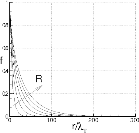
Figure 1: Longitudinal correlation function for different Taylor-Scale Reynolds numbers.

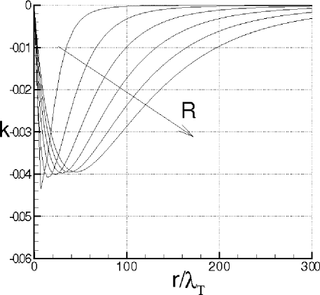
Figure 2: Longitudinal triple correlation function for different Taylor-Scale Reynolds numbers.

The cases here analyzed correspond to $R$=$100$, $200$, $300$, $400$, $500$ and $600$. The fixed step size of the integrator scheme is selected on the basis of the asymptotic stability condition $\Delta\hat{r}=\sqrt{2}/R$ Hildebrand (1987), which also provides a fairly accurate description of the energy spectrum at the large wave-numbers.

Figures 1 and 2 show the numerical solutions of Eqs. (37), where double and triple longitudinal correlation functions are represented in terms of $\hat{r}$, for the different values of $R$. Due to the mechanism of energy cascade, the tail of $f$ rises with $R$ and the maximum of $|k|$ gives the entity of this mechanism. This value is slightly less than 0.05 and agrees quite well with the numerous data of the literature which concern the evolution of the correlation functions. It is apparent that the spatial variations of $k$ correspond to dimensionless scales $\hat{r}$ whose size increases with $R$.

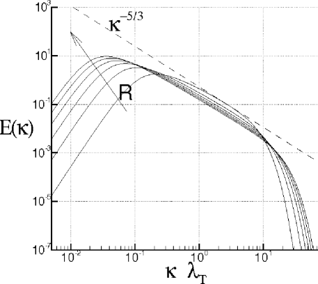
Figure 3: Turbulent Energy Spectrum for different Taylor-Scale Reynolds numbers.

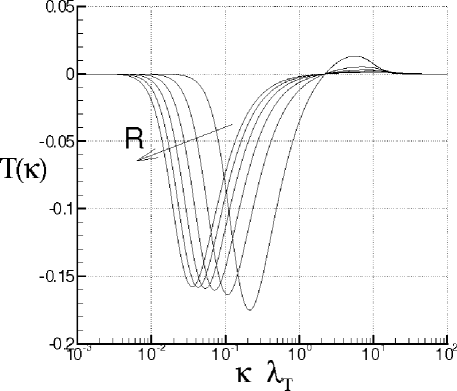
Figure 4: ”Transfer function $T(\kappa)$” for several Taylor-Scale Reynolds numbers.

Figures 3 and 4 show the plots of $E(\kappa)$ and $T(\kappa)$ for the same Reynolds numbers. As the consequence of the mathematical properties of $f$, the energy spectrum behaves like $E(\kappa)=O(\kappa^{4})$ in proximity of the origin, and after a maximum is about parallel to the $-5/3$ Kolmogorov law (dashed line in Fig. 3) in a given interval of the wave-numbers. This interval defines the inertial range of Kolmogorov, and its size increases with $R$. For higher wave-numbers the energy spectrum rapidly decreases with a slope which depends on the behavior of $f$ in proximity of the origin and thus on the Reynolds number.

Since $K$ does not modify the kinetic energy of the flow, according to Eq. (2), the integral of $T(\kappa)$ over the Fourier wave-numbers results to be identically equal to zero at all the Reynolds numbers.

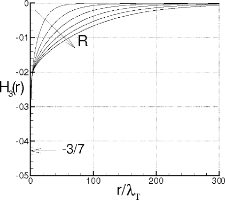
Figure 5: Skewness of $\Delta u_{r}$ at different Taylor-Scale Reynolds numbers.

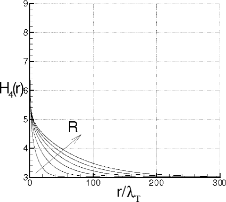
Figure 6: Flatness of $\Delta u_{r}$ at different Taylor-Scale Reynolds numbers.

In the Figs. 5 and 6, skewness and flatness of $\Delta u_{r}$ are shown in terms of $\hat{r}$ for the same values of $R$. The skewness $H_{3}$ is first calculated according to Eq. (4) and thereafter the flatness $H_{4}$ has been determined using Eq. (7). For a given $R$, $|H_{3}|$ starts from 3/7 at the origin, then decreases to small values, while $H_{4}$ starts from values quite greater than 3 at $r=0$, then reaches the value of 3 (faster than $H_{3}$ tending to zero). Although $H_{3}(0)$ does not depend upon $R$, $H_{3}(\hat{r})$ is a rising function of $R$ and, in any case, the intermittency of $\Delta u_{r}$ increases with $R$ according to Eqs. (7) and (8).

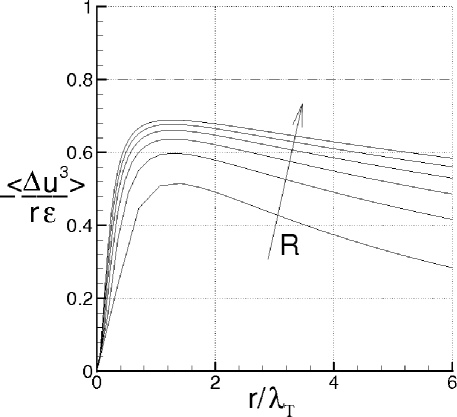
Figure 7: Kolmogorov function for several Taylor-Scale Reynolds numbers.

Next, the Kolmogorov function $Q(r)$ and Kolmogorov constant $C$, are determined using the previous results. According to the theory, the Kolmogorov function, defined as

$$\displaystyle Q(r)=-\frac{\langle(\Delta u_{r})^{3}\rangle}{r\varepsilon}$$ (38)

is constant with respect to $r$, and is equal to 4/5 as long as $r/\lambda_{T}=O(1)$. As shown in Fig. 7, $Q(r)$ exhibits a maximum for $\hat{r}=O(1)$ and quite small variations for higher $\hat{r}$, as the Reynolds number increases. This maximum increases with $R$, and seems to tend toward the limit $4/5$ prescribed by the Kolmogorov theory.

The Kolmogorov constant $C$, defined by $\displaystyle E(\kappa)\approx C{\varepsilon^{2/3}}/{\kappa^{5/3}}$, is here calculated as

$$C=\max_{\kappa\in(0,\infty)}\frac{E(\kappa)\kappa^{5/3}}{\varepsilon^{2/3}}$$ (39)

where $\displaystyle\varepsilon=-3/2\ du^{2}/dt$ is the rate of the energy of dissipation. In the table 1, the Kolmogorov constant is reported in terms of the Taylor-scale Reynolds number.

$R$	$C$
100	1.8860
200	1.9451
300	1.9704
400	1.9847
500	1.9940
600	2.0005

Table 1: Kolmogorov constant for different Taylor-Scale Reynolds number.

The obtained values of $C$ and $Q_{max}$ are in good agreement with the corresponding values known from the various literature.

The spatial structure of $\Delta u_{r}$, expressed by Eq. (7), is also studied with the previous results.

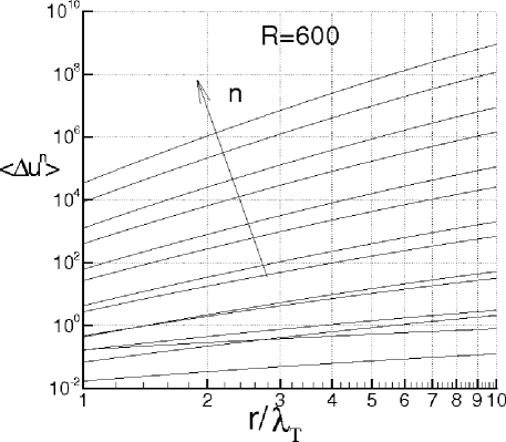
Figure 8: Statistical moments of $\Delta u_{r}$ in terms of the separation distance, for $R$=600.

R	$\zeta(1)$	$\zeta(2)$	$\zeta(3)$	$\zeta(4)$	$\zeta(5)$	$\zeta(6)$	$\zeta(7)$	$\zeta(8)$	$\zeta(9)$	$\zeta(10)$	$\zeta(11)$	$\zeta(12)$	$\zeta(13)$	$\zeta(14)$	$\zeta(15)$
100	0.35	0.70	1.00	1.30	1.56	1.82	2.06	2.31	2.53	2.76	2.97	3.18	3.39	3.59	3.79
200	0.35	0.71	1.00	1.29	1.55	1.81	2.05	2.28	2.50	2.72	2.93	3.14	3.33	3.53	3.73
300	0.35	0.71	1.00	1.29	1.55	1.81	2.05	2.28	2.50	2.73	2.93	3.14	3.34	3.54	3.73
400	0.35	0.71	1.00	1.29	1.55	1.81	2.04	2.28	2.50	2.72	2.93	3.13	3.33	3.53	3.72
500	0.35	0.71	1.00	1.29	1.55	1.81	2.04	2.28	2.50	2.72	2.93	3.13	3.33	3.53	3.73
600	0.35	0.71	1.00	1.29	1.55	1.81	2.05	2.28	2.51	2.73	2.94	3.15	3.35	3.55	3.75

Table 2: Scaling exponents of the longitudinal velocity difference for several Taylor-Scale Reynolds number.

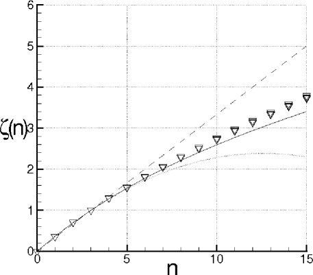
Figure 9: Scaling exponents of $\Delta u_{r}$ for several $R$. Solid symbols are for the present data. Dashed line is for Kolmogorov K41 data Kolmogorov (1941). Dotted line is for Kolmogorov K62 data Kolmogorov (1962). Continuous line is for She-Leveque data She-Leveque (1994)

According to the various works Kolmogorov (1962); She-Leveque (1994); Benzi et al (1991), $\Delta u_{r}$ behaves quite similarly to a multifractal system, where $\Delta u_{r}$ obeys to a law of the kind $\Delta u_{r}(r)\approx r^{q}$ in which $q$ is a fluctuating exponent. This implies that the statistical moments of $\Delta u_{r}(r)$ are expressed through different scaling exponents $\zeta(n)$ whose values depend on the moment order $n$, i.e.

$$\left\langle(\Delta u_{r})^{n}(r)\right\rangle=Ar^{\zeta(n)}$$ (40)

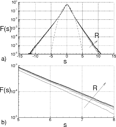
Figure 10: Probability distribution functions of the longitudinal velocity derivative for the different Taylor-Scale Reynolds numbers

In order to calculate these exponents, the statistical moments of $\Delta u_{r}$ are first calculated using Eqs. (7) and (11) for several separation distances. Figure 8 shows the evolution of the statistical moments of $\Delta u_{r}$ in terms of $\hat{r}$, in the case of $R=600$. The scaling exponents of Eq. (40) are identified through a best fitting procedure, in the intervals ($\hat{r}_{1},\hat{r}_{2}$), where the endpoints $\hat{r}_{1}$ and $\hat{r}_{2}$ have to be determined. The calculation of $\zeta(n)$ and $A_{n}$ is carried out through a minimum square method which, for each moment order, is applied to the following optimization problem

$$\displaystyle J_{n}(\zeta(n),A_{n})\equiv\int_{\hat{r}_{1}}^{\hat{r}_{2}}\displaystyle(\langle(\Delta u_{r})^{n}\rangle-A_{n}r^{\zeta(n)})^{2}dr=\mbox{min},\ n=1,2,...$$ (41)

where $(\langle(\Delta u_{r})^{n})\rangle$ are calculated with Eqs. (7), $\hat{r}_{1}$ is assumed to be equal to 0.1, whereas $\hat{r}_{2}$ is taken in such a way that $\zeta(3)$ = 1. The so obtained scaling exponents are shown in Table (2) in terms of the Taylor scale Reynolds number, whereas in Fig. 9 (solid symbols) these exponents are compared with those of the Kolmogorov theories K41 Kolmogorov (1941) (dashed line) and K62 Kolmogorov (1962) (dotted line), and with the exponents calculated by She-Leveque She-Leveque (1994) (continuous curve). Near the origin $\zeta(n)\simeq n/3$, and in general the values of $\zeta(n)$ are in good agreement with the She-Leveque results. In particular the scaling exponents here calculated are lightly greater than those by She-Leveque for $n>$ 8.

The PDFs of $\partial u_{r}/\partial{\hat{r}}$ are determined by means of Eqs. (11) and (7). Specifically, the PDF is calculated with direct simulations, where the sequences of the variables $\xi$, $\eta$ and $\zeta$ are first determined by a gaussian random numbers generator. The distribution function is then calculated through the statistical elaboration of the data obtained with Eq. (7). The results are shown in Fig. 10a and 10b in terms of the dimensionless abscissa

$$\displaystyle s=\frac{\partial u_{r}/\partial{\hat{r}}}{\langle\left(\partial u_{r}/\partial{\hat{r}}\right)^{2}\rangle^{1/2}}$$

These distribution functions are normalized, in order that their standard deviations are equal to the unity. The figure represents the PDF for the several $R$, where the dashed curve represents the gaussian distribution functions. In particular, Fig. 10b shows the enlarged region of Fig. 10a, where $5<s<8$. According to Eq. (7), the tails of PDFs change with $R$ in such a way that the intermittency of $\partial u_{r}/\partial{\hat{r}}$ rises with the Reynolds number.

IV Conclusions

The obtained self–similar solutions of the von Kármán-Howarth equation with the proposed closure, and the corresponding characteristics of the turbulent flow are shown to be in very good agreement with the various properties of the turbulence from several points of view.

In particular:

• The energy spectrum follows the Kolmogorov law in a range of wave-numbers whose size increases with the Reynolds number.

• The Kolmogorov function exhibits a maximum and relatively small variations in proximity of $r=O(\lambda_{T})$. This maximum value rises with the Reynolds number and seems to tend toward the limit $4/5$, prescribed by the Kolmogorov theory.

• The Kolmogorov constant moderately varies with the Reynolds number with an average value around to 1.95 when $R$ varies from 100 to 600.

• The scaling exponents of the moments of velocity difference are calculated through a best fitting procedure in an opportune range of the separation distance. The values of these exponents are in good agreement with the results known from the literature.

• The intermittency of the longitudinal velocity difference rises with the Reynolds number.

These results represent a further test of the analysis presented in Ref. deDivitiis (2009) which adequately describes many of the properties of the isotropic turbulence.

V Acknowledgments

This work was partially supported by the Italian Ministry for the Universities and Scientific and Technological Research (MIUR).

References

- deDivitiis (2009) de Divitiis N., Lyapunov Analysis of Homogeneous Isotropic Turbulence, arXiv:0905.3513 [physics.flu-dyn], 21 May 2009, submitted to Phys. Rev. E.
- Landau (1944) Landau, L. D., , Lifshitz, M., Fluid Mechanics. Pergamon London, England, 1959.
- Karman & Howarth (1938) von Kármán, T. & Howarth, L., On the Statistical Theory of Isotropic Turbulence., Proc. Roy. Soc. A, 164, 14, 192, 1938.
- Batchelor (1953) Batchelor G.K., The Theory of Homogeneous Turbulence. Cambridge University Press, Cambridge, 1953.
- Karman & Lin (1949) von Kármán, T. & Lin, C. C., On the Concept of Similarity in the Theory of Isotropic Turbulence., Reviews of Modern Physics, 21, 3, 516, 1949.
- Hildebrand (1987) Hildebrand F.B., Introduction to Numerical Analysis, Dover Publications, 1987.
- Kolmogorov (1941) Kolmogorov, A. N., Dissipation of Energy in Locally Isotropic Turbulence. Dokl. Akad. Nauk SSSR 32, 1, 19–21, 1941.
- Kolmogorov (1962) Kolmogorov, A. N., Refinement of Previous Hypothesis Concerning the Local Structure of Turbulence in a Viscous Incompressible Fluid at High Reynolds Number, J. Fluid Mech. 12, 82–85, 1962.
- She-Leveque (1994) She Z.S. and Leveque E., Universal scaling laws in fully developed turbulence, Phys. Rev. Lett. 72, 336, 1994.
- Benzi et al (1991) Benzi R., Biferale L., Paladin G., Vulpiani A., Vergassola M., Multifractality in the Statistics of the Velocity Gradients in Turbulence, Phys. Rev. Lett. 67, 2299, 1991.