Preheating and the non-gaussianity of the curvature perturbation

Abstract

The perturbation of a light field might affect preheating and hence generate a contribution to the spectrum and non-gaussianity of the curvature perturbation $\zeta$. The field might appear directly in the preheating model (curvaton-type preheating) or indirectly through its effect on a mass or coupling (modulated preheating). We give general expressions for $\zeta$ based on the $\delta N$ formula, and apply them to the cases of quadratic and quartic chaotic inflation. For the quadratic case, curvaton-type preheating is ineffective in contributing to $\zeta$, but modulated preheating can be effective. For quartic inflation, curvaton-type preheating may be effective but the usual $\delta N$ formalism has to be modified. We see under what circumstances the recent numerical simulation of Bond et al. [0903.3407] may be enough to provide a rough estimate for this case.

I Introduction

As far as we can tell, the observed cosmological perturbations originate from a primordial curvature perturbation $\zeta({\mathbf{x}})$, that is present at the epoch when the shortest cosmological scale approaches horizon entry. That epoch corresponds to a temperature of order $1\,\mbox{MeV}$ and an age $t\sim 1\,\mbox{s}$. At this stage the curvature perturbation is time-independent because the cosmic fluid is radiation-dominated to very high accuracy, but it may be time dependent at earlier times.

It is thought that $\zeta({\mathbf{x}},t)$ at each position is determined by the values $\phi^{*}_{i}({\mathbf{x}})$, of one or more scalar fields evaluated at some initial epoch during inflation. (We shall consistently use a star to denote quantities evaluated at this epoch.) The corresponding perturbations $\delta\phi^{*}_{i}$ are supposed to be generated from the vacuum fluctuation, which requires the fields to be light.

According to the original paradigm, $\zeta$ is generated entirely from the perturbation $\delta\phi_{*}$ of the inflaton field in a slow roll inflation model. In that case, $\zeta$ is present already at the initial epoch, being constant thereafter. The non-gaussianity of $\zeta$ is in this case very small, and almost certainly undetectable.

According to alternative paradigms, the perturbation $\delta\chi_{*}$ of a light field other than the inflaton generates a significant (maybe dominant) contribution. Such a contribution is initially negligible, growing to its final value later, and in general only after inflation is over. The non-gaussianity in this case can be detectable.

In this paper we consider the growth of $\zeta$ that may occur during preheating. Preheating may be defined as the loss of energy by time-dependent scalar fields, through mechanisms other than single particle decay. Preheating is typically followed by reheating, with an intervening era between the two. Reheating may be defined as the practically complete thermalization of a gaseous cosmic fluid, including the case that the constituents of the gas correspond to an oscillating scalar field.

The simplest mechanism for preheating is the potential

$$V=\frac{1}{2}m^{2}\phi^{2}+\frac{1}{2}g^{2}\phi^{2}\chi^{2},$$ (1)

with $\phi$ the inflaton field, and $\chi=0$ during inflation so that we deal with the quadratic (‘chaotic’) inflation potential. If no other terms of the action are relevant, $\phi$ oscillates and loses energy by creating $\chi$ particles through what is called parametric resonance bt ; kls ; bt2 ; kls2 . As in this example, the field $\chi$ is usually different from the field $\phi$, but parametric resonance works in just the same way if they are the same. It also works with different forms of the potential, such as kls3

$$V=\frac{1}{4}\lambda\phi^{4}+\frac{1}{2}g^{2}\phi^{2}\chi^{2},$$ (2)

with again $\phi$ the inflaton field. (That case is often called massless preheating.) Given a potential that allows preheating, it can happen that the produced field $\chi$ can decay sufficiently rapidly into (say) a pair of fermions, so that $\phi$ can lose its energy before even one oscillation takes place. That is called instant preheating fkl . There is also what is known as tachyonic preheating tachyonic , which in its simplest form invokes the potential

$$V(\chi)=V_{0}-\frac{1}{2}m^{2}\chi^{2}+\frac{1}{4}\lambda\chi^{4}.$$ (3)

Tachyonic preheating occurs because the effective mass-squared $-m^{2}$ is initially to be positive. During the sign change of $m^{2}$ the vacuum fluctuation of $\chi$ to be promoted to a classical perturbation which is then amplified as $\chi$ rolls off the hilltop. Parametric resonance can take place is $\chi$ passes through the minimum, followed by more amplification of the original perturbation and so on.

These basic preheating mechanisms have been considered within several different scenarios. In most of them, preheating takes place immediately after inflation so that the oscillating field is the one involved in the inflation model. (If the inflation model is hybrid or multi-field there are two or more of these fields.) In some scenarios though, preheating takes place after a later phase transition and the oscillating field played no role during inflation.

As we will explain, any growth of $\zeta$ occurring during preheating may persist for some time afterwards. The growth will generally terminate at or before reheating. (If there is further growth during or after reheating then that growth should be treated as a separate process.) For clarity we will just talk about ‘growth during preheating’ on the understanding that any subsequent growth prior to reheating is to be included in the discussion.

Regarding its ability to generate a contribution to $\zeta$, preheating has some points of similarity with reheating. Two distinct mechanisms exist in the reheating case. In the original ‘curvaton’ mechanism curvaton1 ; curvaton2 ; curvaton3 ; mollerach ; luw , the light field responsible for generating the contribution to $\zeta$ is the oscillating scalar field, whose decay is responsible for reheating. Later, the ‘modulated reheating’ mechanism was proposed inhomreh ; zaldarriaga . There, the relevant light field acts only indirectly, by affecting the decay rate of the inflaton so that we have $\Gamma(\chi({\mathbf{x}}))$ where that $\Gamma$ is the decay rate and $\chi$ is the perturbed light field. With this in mind, we can distinguish two versions of the preheating scenario. In a ‘curvaton-type preheating’ scenario the light field is directly involved in preheating; either a field created by preheating, or an oscillating field that is responsible for the creation. In a ‘modulated preheating’ scenario the light field instead acts indirectly, by affecting a preheating parameter such as the coupling $g$ in Eq. (1). In that case we have $g(\chi)$ where $\chi$ is the light field.

Modulated preheating or reheating can be implemented within any scenario, but becomes predictive only when one specifies the dependence of the parameter on the field (ie. the function $\Gamma(\chi)$ or $g(\chi)$). Curvaton reheating and curvaton-type preheating are more restricted, but more predictive because $\Gamma$, $g$ and so on are taken to be constants. We shall show that curvaton-type preheating cannot occur with the potential (1) if it is supposed to hold also during inflation.

What we are calling modulated preheating has not so far been studied, though its possibility has been recognized acker . (For related works see batt .) The possibility of what we are calling curvaton-type preheating has been considered in a few papers. The papers anupamkari1 ; anupamkari2 , consider the quadratic inflaton potential (1), taking the potential to be valid also during inflation. The papers anupamkari2 ; anupamkari3 ; barnabycline consider tachyonic preheating. The papers instant consider a multi-field generalization of Eq. (1) with instant preheating. The papers massless1 ; anupamasko ; massless2 ; lev consider the massless preheating scenario of Eq. (2). Reference bdk considers preheating at the end of a hybrid inflation model involving the Higgs field. In these works, preheating starts as soon as inflation is over. In another work cnr the curvaton field causes preheating, when it starts to oscillate long after inflation is over. In johntoni preheating is caused by the oscillation of a flat direction of the MSSM, again long after inflation is over.

Most of the papers cited above use cosmological perturbation theory, at either first order instant ; barnabycline ; johntoni ; bdk or second order anupamkari1 ; anupamkari2 ; anupamkari3 ; anupamasko . We instead use the $\delta N$ formalism ss ; lms ; lr . We begin in Section II by recalling the basic properties of the curvature perturbation. In Section III we carefully set up the $\delta N$ formalism. In Section IV we show that the quadratic potential Eq. (1) cannot provide curvaton-type preheating, contrary to what was assumed in anupamkari1 ; anupamkari2 . In Section V we consider modulated preheating with the quadratic potential. In Section VI we consider curvaton-type preheating the quartic potential (2) (massless preheating). In contrast with other applications of the $\delta N$ formalism, the perturbations of the light fields generated after cosmological scales leave the horizon are likely to be significant in this case. Ignoring them, we show how to use the recent numerical simulation of lev to give an order of magnitude estimate of $f_{\rm NL}$ with the unperturbed value of $\chi_{*}$ set equal to zero. It disagrees with the estimate obtained in anupamasko using second order cosmological perturbation theory. In a concluding section we summarise our finding, and point to future directions for research. In two appendices we extend the discussion of Section IV.

II The curvature perturbation

II.1 Definition and evolution

The non-perturbative definition of the primordial curvature perturbation $\zeta$ is described in for instance newbook , where original references can be found. The components of the metric tensor are smoothed on a comoving scale $R$ and one considers the super-horizon regime $aR>H^{-1}$ where $H\equiv\dot{a}/a$ is the Hubble parameter and $a(t)$ is the scale factor normalised to 1 at present. The energy density $\rho$ and pressure $P$ are smoothed on the same scale. One considers the slicing of spacetime with uniform energy density. The spatial metric is written as

$$g_{ij}({\mathbf{x}},t)\equiv a^{2}(t)e^{2\zeta({\mathbf{x}},t)}\left(Ie^{h}({\mathbf{x}},t)\right)_{ij},$$ (4)

where $h$ is traceless so that $e^{h}$ has unit determinant. The smoothing scale is chosen to be somewhat shorter than the scales of interest, so that the Fourier components of $\zeta$ on those scales is unaffected by the smoothing. The threading of spacetime is taken to be orthogonal to the slicing. The time dependence of the locally defined scale factor $a({\mathbf{x}},t)\equiv a(t)\exp(\zeta)$ defines the rate at which an infinitesimal comoving volume ${\cal V}$ expands: $\dot{\cal V}/{\cal V}=3\dot{a}({\mathbf{x}},t)/a({\mathbf{x}},t)$.

Under the reasonable assumption that the Hubble scale $H^{-1}$ is the biggest relevant distance scale, the energy continuity equation $d({\cal V}\rho)=-Pd{\cal V}$ at each location is the same as in a homogeneous universe; as far as the evolution of $\rho$ is concerned, we are dealing with a family of separate homogeneous universes. With the additional assumption that the initial condition is set by scalar fields during inflation (adopted here), the smoothed $h_{ij}(t)$ is time-independent after smoothing and then the separate universes are homogeneous as well as isotropic.

Since we are working on slices of uniform $\rho$, the energy continuity equation can be written

$$\dot{\rho}(t)=-3\left[H(t)+\dot{\zeta}({\mathbf{x}},t)\right]\left[\rho(t)+P({\mathbf{x}},t)\right].$$ (5)

One write

$$P({\mathbf{x}},t)=P(t)+\delta P({\mathbf{x}},t),$$ (6)

so that $\delta P$ is the pressure perturbation on the uniform density slices, and choose $P(t)$ so that the unperturbed quantities satisfy the unperturbed equation $\dot{\rho}=-3H(\rho+P)$. Then

$$\dot{\zeta}=-\frac{H\delta P}{\rho+P+\delta P}.$$ (7)

This gives $\dot{\zeta}$ if we know $\rho(t)$ and $P({\mathbf{x}},t)$. It makes $\zeta$ time-independent during any era when $P$ is a unique function of $\rho$ earlier ; lms (hence uniform on slices of uniform $\rho$). The pressure perturbation is said to be adiabatic in this case, otherwise it is said to be non-adiabatic.

The key assumption in the above discussion is that in the superhorizon regime certain smoothed quantities (in this case $\rho$ and $P$) evolve at each location as they would in an unperturbed universe. In other words, the evolution of the perturbed universe is that of a family of unperturbed universes. This is the separate universe assumption, that is useful also in other situations newbook .

The primordial curvature perturbation $\zeta$ is directly probed by observation on ‘cosmological scales’ corresponding to roughly $e^{-15}H_{0}^{-1}\lesssim k^{-1}\lesssim H_{0}^{-1}$. These scale begin to enter the horizon when when $T\sim 1\,\mbox{MeV}$. The Universe at that stage is radiation dominated to very high accuracy, implying $P=\rho/3$ and a constant curvature perturbation which we denote simply by $\zeta({\mathbf{x}})$. When cosmological scales are the only ones of interest, one should choose the smoothing scale as $R\sim e^{-15}H_{0}^{-1}$. Unless stated otherwise, we make this choice.

Within a given scenario, $\zeta$ will exist also on smaller inverse wavenumbers, down to some ‘coherence length’ which might be as low as $k^{-1}\sim e^{-60}H_{0}^{-1}$ (the scale leaving the horizon at the end of inflation). If one is interested in such scales, the smoothing scale $R$ should be chosen to be (somewhat less than) the coherence length.

II.2 Correlators

Theories will predict the correlators of cosmological perturbations. The two-point correlator of a perturbation $g({\mathbf{x}})$ is written ${\langle{g({\mathbf{x}}_{1})g({\mathbf{x}}_{2})}\rangle}$ and so on for higher correlators. The bracket basically denotes an ensemble average, with our universe a typical member of the ensemble. If the perturbations originate as a vacuum fluctuation during inflation, the ensemble average is the vacuum expectation value. If the universe is homogeneous this makes the correlators translation invariant, which we will assume.

Given translation invariance, the ergodic theorem holds whereby the bracket can be taken to be a spatial average. Thus ${\langle{g({\mathbf{x}}_{1})g({\mathbf{x}}_{2})}\rangle}$ is the spatial average of $g({\mathbf{x}}_{1})g({\mathbf{x}}_{2})$ at fixed ${\mathbf{x}}_{1}-{\mathbf{x}}_{2}$, within any volume with size $L$ much bigger than $|{\mathbf{x}}_{1}-{\mathbf{x}}_{2}|$. For any finite $L$, the volume average differs from the the ensemble average. The difference is called cosmic variance.

To exploit the translation invariance it is convenient to work with Fourier components $g_{\mathbf{k}}$. Using a box of coordinate size $L$ we have

$$g_{\mathbf{k}} = \int d^{3}xg({\mathbf{x}})e^{-i{\mathbf{k}}\cdot{\mathbf{x}}}.$$ (8)

$$g({\mathbf{x}}) = L^{-3}\sum_{\mathbf{k}}g_{\mathbf{k}}e^{i{\mathbf{k}}\cdot{\mathbf{x}}}\simeq(2\pi)^{-3}\int d^{3}kg_{\mathbf{k}}e^{i{\mathbf{k}}\cdot{\mathbf{x}}}.$$ (9)

Since the box imposes a periodic boundary condition, only the wavenumbers $kL\gg 1$ are physically significant. For them one can use the final equality. According to the ergodic theorem, one can regard ${\langle{g_{{\mathbf{k}}_{1}}g_{{\mathbf{k}}_{2}}}\rangle}$ as an average over the points within a cell of momentum space, up to the cosmic variance.

The dependence of (the loop contributions to) the correlators upon the box size, reflects the fact that the correlators are in position space are spatial averages within the box. Observations are available within the observable universe, with coordinate size of order Except for the low multipoles of the CMB, all observations probe scales $k\gg H_{0}$. To handle them, one should choose the box size as $L=H_{0}^{-1}$ leblond . A smaller choice would throw away some of the data while a bigger choice would make the spatial averages unobservable.

Low multipoles of the CMB anisotropy explore scales of order $H_{0}^{-1}/\ell$ not very much smaller than $H_{0}^{-1}$. To handle them one has to take $L$ bigger than $H_{0}^{-1}$. For most purposes, one should use a box, such that $\ln(LH_{0})$ is just a few (ie. not exponentially large) mybox ; davids ; newbook .

To summarise, the box size should normally be taken as $L=H_{0}^{-1}$. The exception is the case of low CMB multipoles, where one should normally take $L\gg H_{0}^{-1}$ with $\ln(LH_{0})$ not exponentially large. A box satisfying these requirements will be called a minimal box.

The spectrum $P_{g}$ is defined in terms of the two-point correlator by

$${\langle{g_{\mathbf{k}}g_{{{\mathbf{k}}}^{\prime}}}\rangle}=(2\pi)^{3}\delta^{3}({\mathbf{k}}+{\mathbf{k}}^{\prime})P_{g}(k).$$ (10)

One also defines ${\cal P}_{g}(k)\equiv(k^{3}/2\pi^{2})P_{g}(k)$, also called the spectrum. An equivalent expression newbook is

$${\langle{g({\mathbf{y}})g({\mathbf{x}}+{\mathbf{y}})}\rangle}=(2\pi)^{-3}\int d^{3}kP_{g}(k)e^{i{\mathbf{k}}\cdot{\mathbf{x}}},$$ (11)

where the bracket can be regarded as the spatial average with respect to ${\mathbf{y}}$.

The mean-square perturbation, evaluated within a box of size $L$ and smoothed on scale $R$, is

$${\langle{g^{2}({\mathbf{x}})}\rangle}=\int^{R^{-1}}_{L^{-1}}\frac{dk}{k}{\cal P}_{g}(k)\simeq{\cal P}_{g}\ln(L/R).$$ (12)

The final estimate is valid if ${\cal P}_{g}(k)$ is more or less scale-independent as will usually be the case for primordial perturbations. The spectrum of $\partial g/\partial x_{i}$ (the derivative with respect to one of the coordinates) is $k_{i}^{2}{\cal P}_{g}$, hence the mean-square gradient is

$${\langle{(|{\mbox{\boldmath$\nabla$}}g|)^{2}}\rangle}=\int^{R^{-1}}_{L^{-1}}\frac{dk}{k}k^{2}{\cal P}_{g}(k)\simeq\frac{1}{2}{\cal P}_{g}/R^{2}\sim{\langle{g^{2}}\rangle}/R^{2}.$$ (13)

For a gaussian perturbation, the spectrum defines all correlators. The $n$-point correlators vanish for odd $n$, while for even $n$

$${\langle{g_{{\mathbf{k}}_{1}}g_{{\mathbf{k}}_{2}}g_{{\mathbf{k}}_{3}}g_{{\mathbf{k}}_{4}}}\rangle}={\langle{g_{{\mathbf{k}}_{1}}g_{{\mathbf{k}}_{2}}}\rangle}{\langle{g_{{\mathbf{k}}_{3}}g_{{\mathbf{k}}_{4}}}\rangle}+{\langle{g_{{\mathbf{k}}_{1}}g_{{\mathbf{k}}_{3}}}\rangle}{\langle{g_{{\mathbf{k}}_{3}}g_{{\mathbf{k}}_{2}}}\rangle}+{\langle{g_{{\mathbf{k}}_{1}}g_{{\mathbf{k}}_{4}}}\rangle}{\langle{g_{{\mathbf{k}}_{2}}g_{{\mathbf{k}}_{3}}}\rangle},$$ (14)

and so on. For a non-gaussian contribution one has to specify more quantities, starting with the bispectrum $B_{g}$:

$$\langle g_{{\mathbf{k}}_{1}}g_{{\mathbf{k}}_{2}}g_{{\mathbf{k}}_{3}}\rangle = {(2\pi)^{3}}\delta^{3}({\mathbf{k}}_{1}+{\mathbf{k}}_{2}+{\mathbf{k}}_{3})B_{g}(k_{1},k_{2},k_{3})$$ (15)

$$B_{g}(k_{1},k_{2},k_{3}) = {\cal B}_{g}(k_{1},k_{2},k_{3})\left[P_{g}(k_{1})P_{g}(k_{2})+\,{\rm cyclic\ permutations}\right].$$ (16)

The quantity ${\cal B}_{g}$ is called the reduced bispectrum. For $\zeta$ one uses $f_{\rm NL}\equiv(5/6){\cal B}_{\zeta}$.

From observation of the CMB anisotropy and the galaxy distribution, we know that ${\cal P}_{\zeta}(k)$ is almost scale-independent with the value $(5\times 10^{-5})^{2}\sim 10^{-9}$. Also, we know that $\zeta$ is gaussian to high accuracy. Taking $f_{\rm NL}$ to be practically scale independent (‘local’ form) as is predicted by the models that we consider, the bound at $95\%$ confidence level according to the first of curto is $-4<f_{\rm NL}<80$.

III The $\delta N$ formula

III.1 The general formula

Consider now, the analogue of Eq. (4) for a generic slicing:

$$g_{ij}({\mathbf{x}},t)\equiv a^{2}(t)e^{\psi({\mathbf{x}},t)}\tilde{\gamma}_{ij}({\mathbf{x}},t),$$ (17)

where $\tilde{\gamma}$ has unit determinant. Take the initial slice to be flat (meaning that $\psi=0$) and the final slice to be of uniform energy density so that $\psi=\zeta$. This gives lms

$$\zeta({\mathbf{x}},t)=\delta N({\mathbf{x}},t),$$ (18)

where $N$ is the number of $e$-folds of expansion between the initial and final slice. It is independent of the choice of the initial flat slice because the expansion going from one flat slice to another is uniform. By virtue of the separate universe assumption, this formula allows one to calculate $\zeta({\mathbf{x}},t)$ given the evolution of the scale factor in some family of unperturbed universes.

To proceed, we invoke light fields, taken to be canonically normalized. Ignoring mixed derivatives for simplicity, a light field $\phi_{i}$ is defined newbook as one whose effective mass-squared $m_{i}^{2}$ during inflation satisfies

$$|m_{i}^{2}|\ll H^{2},\qquad m_{i}^{2}\equiv\partial^{2}V/\partial\phi_{i}^{2}.$$ (19)

As each scale $k$ leaves the horizon during inflation, the vacuum fluctuation of each light field is converted to a classical perturbation newbook ; ls . At a given epoch during inflation, the classical fields $\phi_{i}({\mathbf{x}})$ are therefore smooth on the horizon scale.

Now we take the initial epoch to be the one when the smoothing scale $R$ leaves the horizon, and make a crucial assumption. At each location, one or more of the light fields provides the initial condition for the evolution of the local scale factor (along with unperturbed quantities including parameters of the field theory and the values of any relevant unperturbed fields). Then we have lr

$$\zeta({\mathbf{x}},t)=\delta N\equiv N(\rho(t),\phi_{1}^{*}({\mathbf{x}}),\phi_{2}^{*}({\mathbf{x}}),\cdots)-N(\rho(t),\phi_{1}^{*},\phi_{2}^{*},\cdots),$$ (20)

where the star denotes the field values at the initial epoch. Since the typical magnitude of a light field perturbation is of order $H_{*}$, we need values of $\phi_{i}({\mathbf{x}})$ in a range $\Delta\phi_{*}\sim(H_{*}/2\pi)$, centred on the unperturbed values $\phi_{*}$.

These initial values $\phi_{i}^{*}({\mathbf{x}})$ are smooth on the scale $R$, and so are the initial values of $\rho$ and $P$. If the subseqent evolution of the light fields were classical, they would remain smooth on the scale $R$, and so would $\rho$ and $P$. In fact, the vacuum fluctuation continues to generate classical field perturbations, so that by the end of inflation they are present on scales $(aH)_{\rm end}^{-1}<k^{-1}<R$. In all known cases except that of massless preheating, these smaller scale perturbations in the light field have little effect on the perturbations in $\rho$ and $P$ on scales of interest $k^{-1}>R$ and so can be ignored. Then, by virtue of the separate universe assumptions, the evolution of $\rho$ and $P$ at each location is the same as in an unperturbed universe, and so is the evolution of $N$. We can evaluate the curvature perturbation by considering a family of unperturbed universes! This is the usual version of the $\delta N$ formalism, which we use except when dealing with massless preheating.

III.2 Power series in the field perturbations

For each field we can write

$$\phi^{*}_{i}({\mathbf{x}})=\phi^{*}_{i}+\delta\phi^{*}_{i}({\mathbf{x}}).$$ (21)

In all cases so far considered, we can expand $N(\rho(t),\phi_{1}^{*}({\mathbf{x}}),\phi_{2}^{*}({\mathbf{x}}),\cdots)$ as a low-order power series about the unperturbed field values:

$$\zeta({\mathbf{x}},t)=\sum_{i}N_{i}(t)\delta\phi^{*}_{i}({\mathbf{x}})+\frac{1}{2}\sum_{i,j}N_{ij}(t)\delta\phi^{*}_{i}({\mathbf{x}})\delta\phi^{*}_{j}({\mathbf{x}})+\ldots,$$ (22)

where a subscript $i$ denotes $\partial/\partial\phi^{*}_{i}$ evaluated at the unperturbed point of field space. To get the observed quantity $\zeta({\mathbf{x}})$ this should be evaluated after the $N_{i}(t)$ and so on settle down to their final values, which we denote simply by $N_{i}$ and so on.

This formula was first given in lr following the non-linear proof in lms of $\zeta=\delta N$. To first order in the field perturbations, the formula and the proof were given in ss , which focuses on the case that $\zeta$ is generated during inflation. Related formulas for the evolution of $\zeta$ during inflation were given in starobinsky (first order) and in sb (non-linear).

The light field perturbations have completely negligible non-gaussianity mald , and their spectrum soon after horizon exit for the scale $k$ is given by newbook

$${\cal P}_{\delta\phi_{i}}(k)\simeq(H_{k}/2\pi)^{2},$$ (23)

where $H_{k}$ can be taken as the value of $H$ at horizon exit. The observed near-gaussianity of $\zeta$ requires that Eq. (22) is well approximated by one or more linear terms, with the field perturbations nearly gaussian. Taking the initial epoch to be just after horizon exit we then have

$${{\cal P}_{\zeta}}(k)\simeq\sum N^{2}_{i}\left(\frac{H_{k}}{2\pi}\right)^{2}.$$ (24)

Assuming that the reduced bispectrum $f_{\rm NL}$ is big enough to be observable (say $|f_{\rm NL}|\gtrsim 1$), it is generated by the quadratic terms, the slight non-gaussianity of the $\delta\phi_{i}$ being negligible. In this case, $f_{\rm NL}$ is almost scale-independent (local form).

III.3 The inflaton contribution to $\zeta$

We will suppose that there is standard slow-roll inflation, which is effectively single-field because only the inflaton field $\phi$ has significant variation during inflation.

The slow-roll approximation gives $V\simeq 3M_{\rm P}^{2}H^{2}$ and $\dot{\phi}\simeq-V^{\prime}/3H$, where $V(\phi)$ is the potential during slow-roll inflation. This gives the well-known relation

$$N(k)=M_{\rm P}^{-2}\int^{\phi(k)}_{\phi_{\rm end}}\frac{V}{V^{\prime}}d\phi,$$ (25)

where $N(k)$ denotes the number of $e$-folds of slow-roll inflation occurring after the epoch of horizon exit for the scale $k^{-1}$. The inflationary potential will determine the field value $\phi_{\rm end}$ at which slow-roll inflation ends.

One usually denotes $N(H_{0})$ simply by $N$. It is determined by the inflationary energy scale $H_{*}$ and the post-inflationary evolution of the scale factor. A typical value, which we adopt, is $N\simeq 55$. For a smaller scale, $N(k)=N-\ln(k/H_{0})$. For the smallest cosmological scale $k_{\rm min}^{-1}$ (enclosing mass $10^{5}M_{\odot}$ or so) $N(k)=N-15=40$. The initial epoch, when the value of $\phi$ is denoted by $\phi_{*}$, can be soon after that. The important feature of Eq. (25) is that it determines the unperturbed field value $\phi_{*}$ and hence ${\cal P}_{\zeta_{\phi}}$, given the inflationary potential and the post-inflationary cosmology.

Perturbing $\phi$ with any other light fields fixed gives a constant contribution $\zeta_{\phi}({\mathbf{x}})$ to $\zeta$, because it represents a shift back and forth along the trajectory which does not alter the subsequent relation between $\rho$ and $P$. The perturbation $\delta\phi_{*}$ has typical magnitude $H_{*}/2\pi\ll\phi_{*}$. Since $\zeta_{\phi}$ represents a shift along the inflaton trajectory, $N_{\phi}=-H/\dot{\phi}$ evaluated at the initial epoch. Using the slow-roll approximation one finds that $\zeta_{\phi}$ is practically linear, making it practically gaussian slfield . Taking the initial epoch soon after horizon exit,

$${\cal P}_{\zeta_{\phi}}(k)=N_{\phi}^{2}(H_{k}/2\pi)^{2}.$$ (26)

If ${\cal P}_{\zeta_{\phi}}$ dominates, the spectral tilt is $n-1=2\eta-6\epsilon$, where $\eta\equiv M_{\rm P}^{2}V^{\prime\prime}/V$ and $\epsilon\equiv M_{\rm P}^{2}(V^{\prime}/V)^{2}/2$ evaluated at horizon exit.

III.4 The non-inflaton contribution

Now we consider the contribution of light fields other than the inflaton. We suppose that only one of them contributes significantly, and call it $\sigma$. Its contribution $\zeta_{\sigma}({\mathbf{x}},t)$ is initially negligible, but it can grow by generating a non-adiabatic pressure perturbation. This might happen during any era, except one of complete matter domination ($P=0$) or complete radiation domination ($P=\rho/3$). Possibilities in chronological order include generation (i) during multi-field inflation starobinsky , (ii) at the end of inflation myend , (iii) during preheating as we discussed in the Introduction, (iv) during modulated reheating inhomreh ; zaldarriaga ; acker ; Suyama:2007 , (v) at a modulated phase transition Matsuda:2009yt and (vi) before a second reheating through the curvaton mechanism luw . In this paper we focus on preheating.

We interested in the value of $\zeta_{\sigma}$ after it settles down to its final constant value, which we denote simply by $\zeta_{\sigma}({\mathbf{x}})$

$$\zeta_{\sigma}({\mathbf{x}}) \equiv \zeta({\mathbf{x}})-\zeta_{\phi}({\mathbf{x}})$$ (27)

$$= \delta N(\sigma_{*}({\mathbf{x}}),\phi_{*})+\delta\left[N(\sigma_{*}({\mathbf{x}}),\phi_{*}({\mathbf{x}})))-N(\sigma_{*}({\mathbf{x}}),\phi_{*})-N(\sigma_{*},\phi_{*}({\mathbf{x}}))\right].$$ (28)

We make the followign approximation, which is usually adequate:

$$\zeta_{\sigma}({\mathbf{x}}) \simeq \delta N(\sigma_{*}({\mathbf{x}}),\phi_{*})$$ (29)

$$\simeq N_{\sigma}\delta\sigma_{*}({\mathbf{x}})+\frac{1}{2}N_{\sigma\sigma}\left(\delta\sigma_{*}({\mathbf{x}})\right)^{2}.$$ (30)

Eq. (29) ignores mixed derivatives $\partial^{2}N/\partial\phi_{*}\partial\sigma_{*}$ and so on, while Eq. (30) ignores $\partial^{3}N/\partial\sigma_{*}^{3}$ and higher derivatives.

The unperturbed value $\sigma_{*}$ is defined as the spatial average of $\sigma({\mathbf{x}})$ within the minimal box. It is in general a free parameter whose value has to be specified along with the parameters of the Lagrangian. To get some idea about is likely value though, we can use the fact that the mean square perturbation, smoothed on scale $L_{1}$ and evaluated within a larger box of size $L_{2}$, is

$$\overline{(\delta\sigma_{*})^{2}}=\int^{L_{1}^{-1}}_{L_{2}^{-1}}\frac{dk}{k}{\cal P}_{\delta\sigma_{*}}(k)\sim(H_{*}/2\pi)^{2}\ln(L_{2}/L_{1}),$$ (31)

where in the final equality we set ${\cal P}_{\sigma_{*}}\sim(H_{*}/2\pi)^{2}$. To use this formula we can take $L_{1}=L$ with $L$ a minimal box centred on the observable universe. Then the formula says that the unperturbed value of $\sigma_{*}$ (ie. it’s spatial average within the minimal box) will be at least of order $H_{*}/2\pi$ if the observable universe is located at a typical position. If there were a very large number of $e$-folds of almost-exponential inflation before the observable universe left the horizon. we can go further; taking the formula literally we can choose $\ln(L_{2}/L_{1})$ to be much bigger than 1, and conclude that the value of the unperturbed field for a typical location of our universe will be much bigger than $H_{*}/2\pi$. (As $\ln(L_{2}/L_{1})$ is increased the calculation leading to Eq. (31) will at some stage become out of control mybox but we don’t need an enormous value of $\ln(L_{2}/L_{1})$ to arrive at the above conclusion.) Of course, it might be that we live in a special place where the the unperturbed $\chi_{*}$ is much less than $H_{*}/2\pi$.

Using Eqs. (8), (10), (14) and (16), and taking $\delta\sigma_{*}$ to be gaussian with a scale-independent spectrum ${\cal P}_{\delta\sigma_{*}}=(H_{*}/2\pi)^{2}$, we can evaluate the spectrum and bispectrum of the curvature perturbation. One finds

$${\cal P}_{\zeta_{\sigma}} = {\cal P}_{\zeta_{\sigma}}^{\rm tree}+{\cal P}_{\zeta_{\sigma}}^{\rm loop}$$ (32)

$${\cal P}_{\zeta_{\sigma}}^{\rm tree} = N_{\sigma}^{2}{\cal P}_{\delta\sigma_{*}}=N_{\sigma}^{2}(H_{*}/2\pi)^{2}$$ (33)

$${\cal P}_{\zeta_{\sigma}}^{\rm loop}(k) = \frac{1}{4}N^{2}_{\sigma\sigma}{\cal P}_{(\delta\sigma_{*})^{2}}(k)=N^{2}_{\sigma\sigma}\ln(kL)\left(\frac{H_{*}}{2\pi}\right)^{4},$$ (34)

and

$$f_{\rm NL} = f_{\rm NL}^{\rm tree}+f_{\rm NL}^{\rm loop}$$ (35)

$$f_{\rm NL}^{\rm tree} = \frac{5}{6}\left(\frac{{\cal P}_{\zeta_{\sigma}}}{{{\cal P}_{\zeta}}}\right)^{2}\frac{N_{\sigma\sigma}}{N_{\sigma}^{2}}$$ (36)

$$f_{\rm NL}^{\rm loop}(k_{1},k_{2},k_{3}) \sim \ln(kL)\frac{N_{\sigma\sigma}^{3}}{{{\cal P}_{\zeta}}^{2}}\left(\frac{H_{*}}{2\pi}\right)^{6}.$$ (37)

The labels ‘tree’ and ‘loop’ refer to the Feynman-like diagrams of bksw . The loop contributions correspond to formally divergent integrals, but they are regularized by setting ${\cal P}_{\zeta_{\sigma}}=0$ for $k\lesssim L^{-1}$, with $L$ the box size. Eq. (34) was given in myaxion . It is valid for $k\gg L^{-1}$, which is anyhow required so that one can ignore the artificial periodicity of the Fourier series. Eq. (36) was first given in fnllocal . Eq. (37) was given in bl , with $k_{i}$ taken to have a common value $k\gg L^{-1}$ to rough order of magnitude.

We see that

$${\cal P}_{\zeta_{\sigma}}^{\rm loop} = \ln(kL)\left(\frac{H_{*}}{2\pi}\frac{N_{\sigma\sigma}}{N_{\sigma}}\right)^{2}{\cal P}_{\zeta_{\sigma}}^{\rm tree},$$ (38)

$$f_{\rm NL}^{\rm loop} \sim \ln(kL)\left(\frac{H_{*}}{2\pi}\frac{N_{\sigma\sigma}}{N_{\sigma}}\right)^{2}f_{\rm NL}^{\rm tree}.$$ (39)

By examining the integral bl leading to Eq. (37), one can see that Eq. (39) becomes exact in the squeezed configuration $k\equiv k_{1}\ll k_{2}\simeq k_{3}$. This has not been noticed before, and is quite interesting because the observational constraint on a local $f_{\rm NL}$ comes mostly from the squeezed configuration curto .

We see that the tree contributions dominate if

$$\ln(kL)\left(\frac{H_{*}}{2\pi}\frac{N_{\sigma\sigma}}{N_{\sigma}}\right)^{2}\ll 1,$$ (40)

while the loop contributions dominate in the opposite case. An equivalent statement is that the tree contributions dominate if the linear term of Eq. (30) dominates, while the loop contributions dominate if the quadratic term of Eq. (30) dominates. (The statements are equivalent because the mean-square of $\delta\sigma_{*}$, smoothed on the scale $k$, is $\ln(kL)(H_{*}/2\pi)^{2}$.)

When comparing the loop contribution with observation one should normally set $L=H_{0}^{-1}$, except for the low CMB multipoles where one should choose $L\gg H_{0}^{-1}$ with $\ln(kL)\sim 1$. With the choice $L=H_{0}^{-1}$, $\ln(kL)\sim 5$ for the scales explored by the CMB multipoles with $\ell\sim 100$, while $\ln(kL)\sim 10$ for the scales explored by galaxy surveys. This increase would be observable leblond .

If $\zeta_{\sigma}\simeq\zeta$ dominates, the near-gaussianity of $\zeta$ requires mybox that the tree contributions dominate. Then, by taking the initial epoch to be soon after horizon exit, one finds spectral tilt

$$n-1=2\eta_{\sigma\sigma}-2\epsilon,$$ (41)

where $\eta_{\sigma\sigma}\equiv M_{\rm P}^{2}(\partial^{2}V/\partial\sigma_{*}^{2})/V$

III.5 Evolution of $\sigma$

As noted earlier, we can usually take the relevant light fields $\phi_{i}({\mathbf{x}},t)$ to be smooth on the scale $R$ even after the initial epoch. Then we can invoke the separate universe assumption, making their evolution at each location the same as in some unperturbed universe. This will give $\sigma(\rho(t),{\mathbf{x}})$ as a function of $\rho(t)$ and $\sigma_{*}({\mathbf{x}})$. Just before $\zeta_{\sigma}$ starts to become significant at some epoch $t_{\rm start}$, this will give some relation $\sigma(\rho(t_{\rm start}),{\mathbf{x}})=g(\sigma_{*}({\mathbf{x}}))$. We can then replace Eq. (29) by myg

$$\zeta_{\sigma}({\mathbf{x}})\simeq\delta N(g(\sigma_{*}({\mathbf{x}})),\phi_{*}).$$ (42)

The derivatives in Eq. (30) are then evaluated using $\partial/\partial\sigma_{*}=(dg/d\sigma_{*})\partial/\partial g$.

As long as $\sigma$ exchanges no energy with its surroundings, its evolution will be given by the field equation

$$\ddot{\sigma}+3H\dot{\sigma}+\partial V/\partial\sigma=0.$$ (43)

This is a good approximation in almost all cases. (An exception within the original curvaton scenario will occur if $\sigma$ loses energy by preheating soon after it begins to oscillate cnr .)

IV Impossibility of curvaton-type preheating with the quadratic potential

IV.1 Inflation

Now we consider preheating with the quadratic potential (1). We assume that the potential holds also during inflation, with the first term dominating so that $V=m^{2}\phi^{2}/2$. Under that assumption, we are going to show that curvaton-type preheating cannot occur, because the small value of $g$ required to make $\chi$ light during inflation is insufficient to cause significant preheating. In Appendix B we show that the same is true if the potential during inflation flattens out corresponding to what is called inflection-point inflation.

With the potential $V=m^{2}\phi^{2}/2$, the inflaton contribution to $\zeta$ gives ${\cal P}_{\zeta_{\phi}}\simeq m^{2}/M_{\rm P}^{2}$. With $m^{2}=10^{-10}M_{\rm P}^{2}$ this contribution dominates, which is allowed by present observations. We will take the value $m^{2}=10^{-10}M_{\rm P}^{2}$ as an order of magnitude estimate. (As will become clear, curvaton-type preheating is excluded even more strongly if $m$ is lower.) Inflation ends when $\phi\sim M_{\rm P}$ making $\phi_{*}^{2}\gg M_{\rm P}^{2}$. Therefore, $\chi$ is light only if $g^{2}\ll m^{2}/M_{\rm P}^{2}\sim 10^{-10}$. We write $g_{5}\equiv g/10^{-5}$, and require $g_{5}\ll 1$.

During inflation the unperturbed fields evolve according to the slow roll approximation:

$$3H\dot{\phi} = -m^{2}(\phi)\phi$$ (44)

$$m^{2}(\phi) \equiv m^{2}+g^{2}\chi^{2}=m^{2}\left(1+g^{2}_{5}\frac{\chi^{2}}{M_{\rm P}^{2}}\right)\simeq m^{2}$$ (45)

$$3H\dot{\chi} = -g^{2}\phi^{2}\chi\simeq-g^{2}_{5}m^{2}\chi,$$ (46)

with $3M_{\rm P}^{2}H^{2}\simeq m^{2}\phi^{2}/2$. We assume $\chi\ll M_{\rm P}$. The evolution of $\phi$ is hardly affected by $\chi$, and well before the end of inflation $N(t)=-\frac{1}{2}\frac{\phi^{2}(t)}{M_{\rm P}^{2}}$, where $N(t)$ is the remaining number of $e$-folds of inflation. Using this expression one finds $\chi(t)\propto[N(t)]^{2g^{2}_{5}}$, which means that $\chi$ is practically constant during inflation.

Inflation ends soon after the slow-roll approximation fails, which in turn happens when $H(t)\simeq m$. After inflation $\phi^{2}$ oscillates, and $\chi(t)=\propto\exp[-g^{2}_{5}N(t)]$, where now $N(t)$ is the number of $e$-folds after the end of inflation. This behavior persists until $\phi$ decays, or the mass of $\chi$ becomes significant. These events must occur in time to create radiation with $T\sim\,\mbox{MeV}$, which means roughly $N(t)\lesssim 10^{2}$. Assuming $g^{2}_{5}\lesssim 10^{-1}$ the evolution of $\chi$ is again negligible. We can therefore set $\chi(t)=\chi_{*}$.

At this point we mention the issue of radiative contributions to the potential, generated by the coupling $g^{2}$. According to the Coleman-Weinberg formula, the one-loop $\xi$ contribution is

$$V_{\rm loop}=g^{2}\frac{\phi^{4}}{32\pi^{2}}\ln(\phi/Q),$$ (47)

where $Q$ is the renormalization scale. To minimize higher order contributions one should choose $Q\sim\phi_{*}$, and then the requirement that $V^{\prime}_{\rm loop}$ and $V^{\prime\prime}_{\rm loop}$ are negligible corresponds to kls2 $g^{2}\ll 4\pi m/\phi_{*}\sim 10^{-5}$. With supersymmetry the loop correction is reduced and it looks as though the small $g$ that we are invoking is safe. Unfortunately though, this estimate of the loop correction is not self-consistent because the renormalization scale must be below the ultra-violet cutoff of the effective field theory, which in turn must be below $M_{\rm P}$ since we are assuming Einstein gravity. To bring the loop correction under control one would have to embed the model within a larger theory. We proceed on the assumption that the loop correction is negligible.

IV.2 Creation of $\chi$ particles

In the literature, the potential (1) is usually considered with $g^{2}$ not too many orders of magnitude below 1. Then the oscillation of $\phi$ after inflation leads to the copious production of $\chi$ particles. This occurs through what is called parametric resonance, and it rapidly drains away most of the oscillation energy corresponding to what is called preheating. We are going to show that $g^{2}$ is too small for parametric resonance. Then we will show that the variation of $\phi$ around the end of inflation still creates some $\chi$ particles, and go on to estimate the contribution of this creation to $\zeta_{\chi}$.

It is sufficient to consider narrow resonance, which requires the condition $q\equiv g^{2}\overline{\phi^{2}}/4m^{2}\ll 1$. (The alternative regime of broad resonance, $q\gtrsim 1$ requires a bigger value of $g^{2}$.) Narrow resonance occurs if there is time for $\phi$ to undergo some oscillations, while the wavenumber $k/a(t)$ passes through the narrow band

$$1-q(t)/2<\frac{2}{m}\frac{k}{a(t)}<1+q(t)/2.$$ (48)

The time for the passage to occur is $\Delta t\simeq q/2H$, so narrow resonance requires $mq/H\gg 1$. When the oscillation begins at $H=H_{*}\simeq m$, this corresponds to $g^{2}_{5}\gg 1$. Afterwards $\Delta t$ decreases like $a^{-3/2}$. It follows that narrow resonance requires $g^{2}_{5}\gg 1$, which contradicts the light field requirement $g^{2}_{5}\ll 1$. Hence the light field requirement is incompatible with parametric resonance. The estimates of non-gaussianity from preheating in anupamkari1 ; anupamkari2 are therefore inconsinstent, because they invoke both parameteric resonance and the assumption that $\chi$ is light.

The preheating process operates on scales that never leave the horizon. It occurs because the evolution of the mode function $\chi_{k}$ is non-adiabatic. At some level, the evolution of the mode function will be non-adiabatic even if $g^{2}$ is too small for preheating, which means that $\chi$ particles will still be created. Let us see if this creation can give a significant contribution to $\zeta$.

We work with $f_{k}\equiv a\chi_{k}$ and conformal time $\eta$. Denoting $d/d\eta$ by a prime, it satisfies bt

$$f_{k}^{\prime\prime}+\left[k^{2}-X^{2}(\eta)\right]f_{k}=0,\qquad X^{2}\equiv a^{\prime\prime}/a-g^{2}\phi^{2}a^{2}$$ (49)

To calculate the occupation number one imposes the early time condition $\sqrt{2k}f_{k}=\exp(-ik\eta)$. The late time behavior is then

$$\sqrt{2k}f_{k}=\alpha_{k}e^{-ik\eta}+\beta_{k}e^{ik\eta},$$ (50)

with $|\alpha_{k}|^{2}-|\beta_{k}|^{2}=1$, and the occupation number is $n_{k}=|\beta_{k}|^{2}$.

We set $\eta=0$ at the end of inflation. Well before the end of inflation, $\eta=-1/aH_{\rm end}$ and well afterwards $\eta=2/aH$. In both of these regimes, $|\eta|\gg 1/a_{\rm end}H_{\rm end}$ where the star denotes the end of inflation, and we have $X^{2}\simeq a^{\prime\prime}/a\simeq 2/\eta^{2}$. We conclude that $X^{2}$ has a peak centered on $\eta=0$ with width of order $1/a_{\rm end}H_{\rm end}$, and that within the peak, $X^{2}\simeq a^{\prime\prime}/a\sim 1/(a_{\rm end}H_{\rm end})^{2}$. As an approximation we may write

$$a^{\prime\prime}/a\sim 2/[\eta^{2}+(1/a_{\rm end}H_{\rm end})^{2}],$$ (51)

which becomes accurate in the regime $|\eta|\gg 1/(a_{\rm end}H_{\rm end})^{2}$.

In the regime $k\gg a_{\rm end}H_{\rm end}$, the square bracket in Eq. (49) is close to $k^{2}$ at all times, giving $n_{k}\ll 1$. In the opposite regime $k\ll a_{\rm end}H_{\rm end}$, which we are not considering at the moment, the vacuum fluctuation is promoted to a classical perturbation corresponding to occupation number $n_{k}\gg 1$. It follows that in the regime $k\gtrsim a_{\rm end}H_{\rm end}$ under consideration, particle creation occurs mainly at the bottom end of the range corresponding to $k\sim a_{\rm end}H_{\rm end}$ and that $n_{k}\sim 1$ in this range. Assuming that these particles dominate $\rho_{\chi}$ we have

$$3P_{\chi}=\rho_{\chi}\sim\frac{1}{a^{4}}\int_{0}^{\infty}dkk^{3}n_{k}\sim H_{\rm end}^{4}\left(\frac{a_{\rm end}}{a}\right)^{4}.$$ (52)

(We present in an Appendix estimates of $n_{k}$ at $k\gg a_{\rm end}H_{\rm end}$, showing that the contribution from this regime is indeed negligible.) These fall like $a^{-4}$ since we are taking $\chi$ to be massless and the creation occurs at $a\sim a_{\rm end}$. The total energy density is dominated by

$$\rho_{\phi}\sim M_{\rm P}^{2}H_{\rm end}^{2}(a_{\rm end}/a)^{3}.$$ (53)

IV.3 Estimating the contribution to $\zeta_{\chi}$

The contribution $\zeta_{\chi}({\mathbf{x}},t)$ is given by Eq. (30) with $\sigma=\chi$. It is negligible just when the smoothing scale leaves the horizon, which we are choosing to be a bit shorter than the shortest cosmological scale. This epoch is 50 or so $e$-folds before the end of inflation, and we denote it by a subscript 1.

During inflation, $\zeta_{\chi}({\mathbf{x}},t)$ will increase slightly, because the presence of $\chi$ means that there are really two slowly rolling fields. Because we are choosing $g^{2}_{5}\ll 1$ and $\chi\ll M_{\rm P}$, this effect is negligible. We are interested in the possible increase of $\zeta_{\chi}({\mathbf{x}},t)$ shortly after inflation, due to the creation of the $\chi$ particles. We will denoting this increase by $\tilde{\zeta}_{\chi}$. It is equal to $\delta\tilde{N}$, where $\tilde{N}$ is the number of $e$-folds taking place while the $\chi$ particles are being created.

Using Eq. (7) to first order in $\delta P$, we have

$$\frac{\partial\tilde{\zeta}_{\chi}}{\partial\chi_{*}}=\frac{\partial\tilde{N}}{\partial\chi_{*}}=\int^{a_{2}}_{a_{\rm end}}\frac{\partial P/\partial\chi_{*}}{\rho+P}\frac{da}{a},$$ (54)

where a subscript 2 indicates an epoch just after the end of preheating. Without the tildes and with the integration going from the initial epoch to a sufficiently late time, this expression gives the complete quantity $\partial\zeta\chi/\partial\chi_{*}$. It has not been given before. Note that $\chi_{*}$ is evaluated at the initial epoch during the inflation as discussed after Eq. (22).

To evaluate $\partial P/\partial\chi_{*}$, we use Eqs. (53) and (52) for $\rho$ and $P$. They depend on $\chi_{*}$ because the epoch at which inflation ends depends on the effective inflaton mass $m$, which in turn depends slightly on $\chi_{*}$ according to the expression $H_{\rm end}^{2}\simeq m^{2}(\chi_{*})$. Inserting this expression into Eqs. (53) and (52), and differentiating at constant $\rho$, we find

$$\frac{\partial P}{\partial(m^{2})}=-\frac{2}{9}H_{\rm end}^{2}\left(\frac{a_{\rm end}}{a}\right)^{4}.$$ (55)

Using $\partial(m^{2}(\chi_{*}))/\partial\chi_{*}=g^{2}\chi_{*}$ and Eq. (54) we find

$$\frac{\partial N}{\partial\chi_{*}}\sim-\frac{g^{2}\chi_{*}}{M_{\rm P}^{2}}=g^{2}_{5}\frac{m^{2}\chi_{*}}{M_{\rm P}^{4}}.$$ (56)

From these expressions we find

$${\cal P}_{\zeta_{\chi}}/{\cal P}_{\zeta_{\phi}}\sim({g^{2}_{5}})^{4}\left(\frac{m}{M_{\rm P}}\right)^{4}\left(\frac{\chi_{*}}{M_{\rm P}}\right)^{2}\ll\left(\frac{m}{M_{\rm P}}\right)^{4}\sim 10^{-20}.$$ (57)

Assuming $\chi_{*}\gg H_{\rm end}$ the contribution of $(\delta\chi_{*})^{2}$ to the non-gaussianity parameter is given by Eq. (36)

$$\frac{6}{5}f_{\rm NL}^{\chi}=\left(\frac{{\cal P}_{\zeta_{\chi}}}{{\cal P}_{\zeta_{\phi}}}\right)^{2}\frac{\partial^{2}N/\partial\chi_{*}^{2}}{(\partial N/\partial\chi_{*})^{2}}\sim(g^{2}_{5})^{6}\left(\frac{m}{M_{\rm P}}\right)^{6}\left(\frac{\chi_{*}}{M_{\rm P}}\right)^{2}\ll\left(\frac{m}{M_{\rm P}}\right)^{6}\sim 10^{-30}.$$ (58)

If instead $\chi_{*}\lesssim H_{\rm end}$ the result for $f_{\rm NL}^{\chi}$ is even smaller, given by Eq. (37).

Of course this is not the only contribution to $f_{\rm NL}$. The contribution $N_{\chi}\delta\chi_{*}$ will contribute fieldnong because the bispectrum of $\delta\chi_{*}$ is not exactly zero slfield . The dominant contribution though will be from the inflaton perturbation, giving mald ; slfield $|f_{\rm NL}|\sim 10^{-2}$.

V Modulated preheating with the quadratic potential

To generate significant preheating with the quadratic potential (1), we need $g^{2}\gg 10^{-10}$. This makes $\chi$ heavy during inflation, and for preheating to generate a significant contribution to $\zeta$ we need to introduce a third field $\sigma$. The contribution of $\sigma$ to the potential should be such that (i) $\sigma$ is light during inflation and (ii) its value contributes to the effect value of $g$ so that we have $g(\sigma_{*})$. Then the perturbation $\delta\sigma$ on cosmological scales will give a non-adiabatic pressure perturbation between the end of inflation and reheating, which will generate a contribution to $\zeta$. This scenario is similar to the modulated reheating scenario inhomreh ; zaldarriaga ; acker , where the decay rate $\Gamma(\sigma_{*})$ depends on a light field $\chi$. For comparison, we recall the modulated reheating result, using the $\delta N$ formalism newbook .

V.1 Modulated reheating

For modulated reheating it is a good approximation to take the decay as instantaneous. Then $\zeta_{\chi}$ vanishes before decay and is constant thereafter. It can easily be calculate because the dependence of the local scale factor is known both before and after decay inhomreh ; zaldarriaga ; acker ; newbook . Before decay there is matter domination with $a\propto H^{-1/2}$. The decay occurs when $H=\Gamma$, therefore

$$\frac{a_{\rm dec}}{a_{\rm i}}\propto\Gamma^{-2/3},\qquad\frac{a_{\rm f}}{a_{\rm dec}}\propto\Gamma^{1/2}.$$ (59)

This gives $e^{N}\propto\Gamma^{-\alpha}$ with $\alpha=1/6$. Then

$$\frac{\partial N}{\partial\Gamma}=-\alpha\frac{1}{\Gamma},\qquad\frac{\partial^{2}N}{\partial\Gamma^{2}}=\alpha\frac{1}{\Gamma^{2}}.$$ (60)

This gives newbook

$$N_{\sigma}=-\alpha\Gamma^{\prime}/\Gamma,\qquad N_{\sigma\sigma}=-\alpha\Gamma^{\prime\prime}/\Gamma+\alpha\left(\Gamma^{\prime}/\Gamma\right)^{2},$$ (61)

and

$${\cal P}_{\zeta_{\sigma}}=\left(\alpha\frac{\chi_{*}\Gamma^{\prime}}{\Gamma}\right)^{2}\left(\frac{H_{*}}{2\pi\sigma_{*}}\right)^{2},\qquad\frac{6}{5}f_{\rm NL}=-\left(\frac{{\cal P}_{\zeta_{\sigma}}}{{{\cal P}_{\zeta}}}\right)^{2}\alpha\left[\frac{\Gamma^{\prime\prime}\Gamma}{\Gamma^{\prime 2}}-1\right].$$ (62)

For illustration, one may take a simple possibility acker :

$$g^{2}(\sigma_{*})=g^{2}\left(1+\frac{\sigma_{*}^{2}}{M^{2}}\right),\qquad g(\sigma_{*})\simeq g\left(1+\frac{1}{2}\frac{\sigma_{*}^{2}}{M^{2}}\right)\simeq g.$$ (63)

with $M$ some mass scale. Then

$${\cal P}_{\zeta_{\chi}}^{1/2} \sim \alpha\frac{\sigma_{*}}{M^{2}}\left(\frac{H_{*}}{2\pi}\right)$$ (64)

$$f_{\rm NL} \sim \alpha\left(\frac{{\cal P}_{\zeta_{\sigma}}}{{{\cal P}_{\zeta}}}\right)^{2}\left(1-\frac{M^{2}}{2\chi_{*}^{2}}\right).$$ (65)

These expressions allow $\zeta_{\sigma}$ to dominate and they allow $f_{\rm NL}$ to be much bigger than 1.

Figure 1: $f_{\rm NL}$ in the plane of $\chi/M$ and $M$ in case of $g^{2}=10^{-7}$. We plotted $f_{\rm NL}=-10^{-2},-0.1,-1$ and $-10$ from top to bottom. The boundary ${\cal P}_{\zeta_{\sigma}}\leq{\cal P}_{\zeta,{\rm obs}}$ ( $\sim 3\times 10^{-9}$) is also plotted by the solid line.

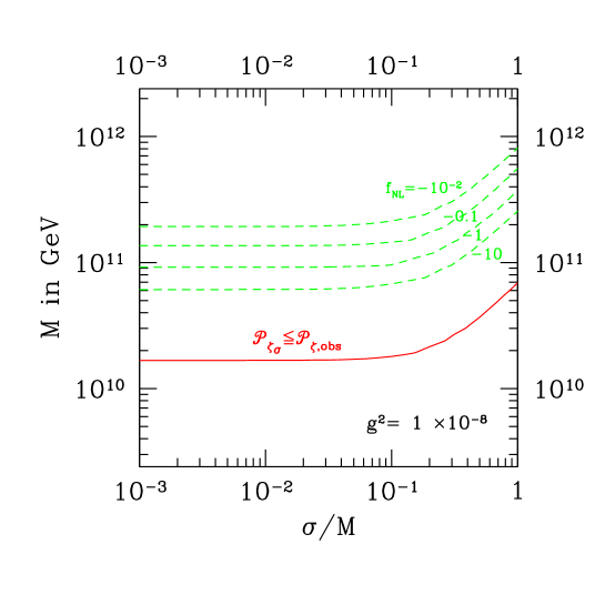
Figure 2: Same as Fig. 1 but for $g^{2}=10^{-8}$

V.2 Modulated preheating

Preheating generates a contribution to $\zeta$ which changes continuously during preheating, and continues to change afterwards for as long as $P_{\chi}$ generates a significant non-adiabatic pressure perturbation. We have therefore

$$\zeta_{\sigma}=\delta N=\delta N_{\rm pre}+\delta N_{\rm after},$$ (66)

where $N_{\rm pre}$ is the number of $e$-folds of preheating and $N_{\rm after}$ is the subsequent number of $e$-folds up to an epoch when the non-adiabatic pressure has become negligible.

Given $N(\sigma_{*})$ we have

$$N_{\sigma} = g^{\prime}\frac{\partial N}{\partial g}$$ (67)

$$N_{\sigma\sigma} = g^{\prime\prime}\frac{\partial N}{\partial g}+{g^{\prime}}^{2}\frac{\partial^{2}N}{\partial g^{2}}.$$ (68)

Inserting these formulas into Eqs. (1) and (37) gives the preheating contribution to the spectrum and non-gaussianity of the curvature perturbation.

For simplicity, we will assume that $\rho_{\chi}$ has almost redshifted when $\phi$ decays, so that the non-adiabatic pressure has become negligible by that time. Since $\rho_{\phi}\propto a^{-3}$ after preheating is over, this gives

$$N_{\rm after}({\mathbf{x}},t)=\frac{1}{3}\ln\left(\frac{\rho_{\phi 2}}{\rho(t)}\right),$$ (69)

where the subscript 2 indicates the end of preheating and $t$ can be taken as the time just before $\phi$ decays. We then have

$$3\frac{\partial N_{\rm after}}{\partial g}=\frac{1}{\rho_{\phi 2}}\frac{\partial\rho_{\phi 2}}{\partial g},$$ (70)

In general, an accurate calculation of $\rho_{\phi 2}$ and $N_{\rm pre}$ requires numerical simulation. Here we will just use analytic estimates kls2 , which should be good in the regime $10^{-10}<g^{2}<10^{-7}$. In this regime, $\rho_{\chi 2}\lesssim\rho_{\phi 2}$, with the equality attained for $g^{2}\sim 10^{-7}$.

According to kls2 , the $\chi$ particles are non-relativistic during preheating. Hence $\rho_{\chi}$ as well as $\rho_{\phi}$ is matter-dominated during this era and the total energy density is proportional to $a^{-3}$. According to kls2 , preheating ends at the epoch given by

$$(mt_{2})^{2}\sim\left(\frac{a_{2}}{a_{\rm end}}\right)^{3}\sim\left(\frac{gM_{\rm P}}{m}\right)^{2}=g_{5}^{2},$$ (71)

where $t_{2}=g\sqrt{8\pi}M_{\rm P}/3m^{2}$ and $g_{5}\equiv g/10^{-5}$. Let us check that the $\chi$ particles are indeed non-relativistic up to this epoch. Their effective mass-squared is

$$m_{\chi}^{2}(t)=g^{2}\overline{\phi^{2}}\sim g^{2}M_{\rm P}^{2}(a_{\rm end}/a(t))^{3}\ ,$$ (72)

where the star denotes the end of inflation. According to kls2 , the momentum of the $\chi$ particles in our regime is kls2 $k/a\sim\sqrt{gM_{\rm P}m}(a_{\rm end}/a)$. It follows that the $\chi$ particles are non-relativistic until

$$(a/a_{\rm end})\sim g\frac{M_{\rm P}}{m}=g_{5},$$ (73)

which is after the end of preheating.

From Eq. (71) we get

$$\frac{\partial N_{\rm pre}}{\partial g}=\frac{2}{3g},\qquad\frac{\partial^{2}N_{\rm pre}}{\partial g^{2}}=-\frac{2}{3g^{2}}.$$ (74)

To handle $N_{\rm after}$ we need $\rho_{\phi}^{\rm end}(g)$. The total energy density at the end of preheating follows from Eq. (71):

$$\rho_{\rm end}\sim M_{\rm P}^{2}m^{2}(a_{\rm end}/a_{2})^{3}\sim m^{4}/g^{2}.$$ (75)

Section IXA of kls2 nicely gives the expression of $n_{\chi}(t)$ for $t<t_{\rm end}$. Multiplying it by $m_{\chi}(t)$ to get $\rho_{\chi}$, we find at the end of preheating

$$\rho_{\chi 2}(g)=Ag^{-1}e^{Bg},$$ (76)

with

$$A = \frac{3^{5/2}\times 10^{-4}m^{5}}{\sqrt{8\pi}\mu^{1/2}M_{\rm P}}$$ (77)

$$B = 2\times(8\pi)^{1/2}\times 0.14M_{\rm P}/m\simeq M_{\rm P}g/m.$$ (78)

The difference between Eqs. (76) and (75) gives $\rho_{\phi}^{\rm end}(g)$, from which we can calculate $\partial N_{\rm after}/\partial g$ and $\partial^{2}N_{\rm after}/\partial g^{2}$ as follow,

$$\frac{\partial N_{\rm after}}{\partial g}=\frac{1}{3(\rho^{\rm end}-\rho^{\rm end}_{\chi})}\left(-\frac{2\rho^{\rm end}}{g}-B\rho^{\rm end}_{\chi}\right),$$ (79)

$$\frac{\partial^{2}N_{\rm after}}{\partial g^{2}}=\frac{1}{3}\left[\frac{-1}{(\rho^{\rm end}-\rho^{\rm end}_{\chi})^{2}}\left(-\frac{2\rho^{\rm end}}{g}-B\rho^{\rm end}_{\chi}\right)^{2}+\frac{1}{(\rho^{\rm end}-\rho^{\rm end}_{\chi})}\left(\frac{6\rho^{\rm end}}{g^{2}}-B^{2}\rho^{\rm end}_{\chi}\right)\right].$$

Adding these into (74), we obtain the total ${\partial N}/{\partial g}$ and ${\partial^{2}N}/{\partial g^{2}}$.

Except near the top of our range $10^{-10}<g^{2}<10^{-7}$, the ratio $R_{\chi}\equiv\rho_{\chi}^{\rm end}/\rho_{\rm end}$ is much less than 1. To first order in $R_{\chi}$ we find simply

$$\frac{\partial N}{\partial g} \simeq -(M_{\rm P}/m)R_{\chi}\simeq-10^{5}R_{\chi}$$ (81)

$$\frac{\partial^{2}N}{\partial g^{2}} \simeq -(M_{\rm P}/m)^{2}R_{\chi}\simeq-10^{10}R_{\chi}.$$ (82)

Taking $g(\chi_{*})$ to be given by Eq. (63) we can calculate ${\cal P}_{\zeta_{\chi}}$ and $f_{\rm NL}$ from Eqs. (32)–(37). In the regime where either of them may be significant, the loop contributions dominate. Setting $\ln(kL)=1$ we plot the result in Figures 1 and 2. (The exact result was used instead of Eqs. (81) and (82), which is needed for Figure 1.) We see that the observational bound $f_{\rm NL}\gtrsim-10$ can be satisfied only if ${\cal P}_{\zeta_{\chi}}/{{\cal P}_{\zeta}}$ is very small.

VI Massless preheating

In this section we consider curvaton-type preheating with the potential (2), usually called massless preheating. Curvaton-type preheating, corresponding to a contribution $\zeta_{\chi}$, is indeed possible for this case, because there is a region of parameter space which makes $\chi$ light during inflation. Also, the inflaton trajectory can be in practically the $\phi$ direction. Then we we deal with single-field inflation, and the contribution $\zeta_{\chi}$ becomes significant only after inflation is over, ie. the preheating contribution to $\zeta_{\chi}$ is the dominant one.

With the potential $V=\lambda\phi^{4}/4$, the inflaton contribution to $\zeta$ gives treview ; newbook ${\cal P}_{\zeta_{\phi}}=10^{3}\lambda$. To agree with observation it should not dominate wmap5 which requires $\lambda\lesssim 10^{-12}$. To obtain significant preheating one requires roughly $g^{2}\sim\lambda$. These small couplings beg explanation, and as with the quadratic potential there is also the issue of keeping radiative contribution to the potential under control (though the naive estimate $V_{\rm loop}\sim g^{4}\phi^{4}\ln(\phi/Q)$ makes that contribution tiny). We proceed without addressing these issues.

VI.1 Inflation

To keep things simple we will pretend that all cosmological scales leave the horizon 55 $e$-folds before the end of inflation, and denote their values then by a subscript 55. Following lev we focus on the case $g^{2}=2\lambda$ (corresponding to a supersymmetry).

Single field inflation occurs if $\partial V/\partial\phi\gg\partial V/\partial\chi$, which corresponds to $\chi\ll\phi$. We assume this condition after the biggest cosmological scale leaves the horizon, which occurs when $\phi\sim 10M_{\rm P}$. Then, during inflation and for some time afterwards,

$$\ddot{\phi}+3H\dot{\phi}+\lambda\phi^{3}=0,$$ (83)

with $H^{2}=\lambda\phi^{4}/12M_{\rm P}^{2}$ during inflation. Inflation ends at the epoch $\phi_{\rm end}\simeq M_{\rm P}$. During inflation, $\eta_{\chi\chi}=4M_{\rm P}^{2}/\phi^{2}$, so that $\chi$ is light except near the end of inflation.

In the slow-roll approximation, the evolution of the fields is given by

$$-\frac{\dot{\phi}}{H} = \frac{\lambda\phi^{3}}{3H^{2}}=4\frac{M_{\rm P}^{2}}{\phi}$$ (84)

$$-\frac{\dot{\chi}}{H} = \frac{g^{2}\phi^{2}\chi}{3H^{2}}=\frac{4}{3}\frac{g^{2}}{\lambda}\frac{M_{\rm P}^{2}\chi}{\phi^{2}}.$$ (85)

Well before the end of inflation, these give

$$\phi(t)\simeq\sqrt{8N(t)}\phi_{\rm end}\qquad\chi(t)=(8N(t))^{g^{2}/6\lambda}\chi_{\rm end},$$ (86)

where $N(t)$ is the remaining number of $e$-folds of inflation. The earliest epoch of interest is the one when the scale $k=H_{0}$ leaves the horizon, corresponding to $N(t)\simeq 55$. Then

$$\phi_{55}\simeq 21\phi_{\rm end}\qquad\chi_{55}\simeq 8\chi_{\rm end}.$$ (87)

The corresponding Hubble parameter is $H_{55}\simeq 440H_{\rm end}$. An accurate calculation personal , taking account of the failure of slow roll near the end of inflation gives $\chi_{55}\simeq 10^{2}\chi_{\rm end}$.

VI.2 Preheating in an unperturbed universe

The field equations are

$$\ddot{\phi}+3H\dot{\phi}+\lambda\phi^{3}+g^{2}\phi\chi^{2} = a^{-2}\nabla^{2}\phi$$ (88)

$$\ddot{\chi}+3H\dot{\chi}+g^{2}\phi^{2}\chi = a^{-2}\nabla^{2}\chi.$$ (89)

In the regime $\chi_{*}\ll\phi_{*}$, the first order perturbation of Eq. (89) gives

$$\ddot{\chi}_{\mathbf{k}}+3H\dot{\chi}_{\mathbf{k}}+g^{2}\phi^{2}\chi_{\mathbf{k}}+(k/a)^{2}\chi_{\mathbf{k}}=0.$$ (90)

In the early stage of preheating, $\phi$ oscillates according to Eq. (83). This corresponds to a time-averaged $P=\rho/3$ (not to $P\ll\rho$ as for the quadratic potential). The broad resonance band of $k$ is time-independent (not redshifted as for quadratic inflation) and depends only on the combination $g^{2}/\lambda$. For cosmological scales to be in the band, it has to extend down to $k=0$. That is the case for $1<g^{2}/\lambda<3$, which is satisfied by our choice $g^{2}=2\lambda$. There is no significant preheating for $g^{2}<\lambda$.

As we noted earlier, $\zeta\simeq\zeta_{\phi}$ is forbidden in this model. In the opposite case $\zeta_{\chi}\simeq\zeta$, the spectral index is given by Eq. (41). In the slow-roll approximation (86) with $\chi=0$ this gives

$$n-1\simeq 0.02\frac{50}{N}\left(\frac{g^{2}}{2\lambda}-1\right).$$ (91)

This too is forbidden by observation with our chosen value $g^{2}=2\lambda$ but it might agree with the minimum value $g^{2}=\lambda$. Otherwise we would need to assume both $\zeta_{\phi}\ll\zeta$ and $\zeta_{\chi}\ll\zeta$, requiring a third light field to give the dominant contribution to $\phi$.

To arrive at an estimate of $\zeta_{\chi}$, we will invoke lev which computes the number $N_{\rm pre}(\chi_{\rm end},\phi_{\rm end})$ of $e$-folds of preheating in a universe that is unperturbed at the end of inflation. To be more precise, $N_{\rm pre}(\chi_{\rm end},\phi_{\rm end})$ is the number of $e$-folds from the end of inflation (when $\dot{H}=-H^{2}$) to an epoch of fixed $\rho$ soon after the end of preheating which is around five $e$-folds later.

The calculation is done within a comoving box, whose size at the end of inflation is $20/H_{\rm end}$, with $H_{\rm end}/2\pi=10^{-7}\times\sqrt{8\pi M_{\rm P}}$. The lowest wavenumber is then $k=(\pi/10)(aH)_{\rm end}$, which means that all $k$ come inside the horizon soon after preheating begins.

Two methods of calculation were used, which give similar results lev ; personal . One of them uses two stages personal . The first stage, lasting for about two $e$-folds, is done in Fourier space. The $k=0$ mode is evolved using the non-linear equations (88) and (89) (with the right hand sides zero). The $k\neq 0$ modes are evolved analytically using Eqs. (83) and (90). Before each such mode leaves the horizon, it is treated quantum mechanically so that Eq. (83) applies to the mode function. In this way, the vacuum fluctuation present before horizon exit becomes a classical perturbation after horizon exit. Up to some $k_{\rm max}$ there is parameteric resonance generating classical perturbations from the vacuum fluctuation. The second stage is a numerical simulation of Eqs. (88) and (89) using a new code Hlattice. The other method does the numerical simulation from the beginning, using an update of the existing code DEFROST frolov .

The result using DEFROST is presented in Figure 1. of lev , with $\phi_{\rm end}$ fixed at the value corresponding to $\epsilon=1$ and with $\chi_{\rm end}$ in the range $10^{-7}M_{\rm P}\lesssim\chi_{\rm end}\lesssim 10^{-4}M_{\rm P}$. In accordance with earlier (but not sufficiently accurate) work kls3 ; massless2 , it is found that $N_{\rm pre}(\chi_{\rm end},\phi_{\rm end})$ is not smooth function of $\chi_{\rm end}$, but rather exhibits sharp spikes. There are big spikes having a spacing of order $H_{\rm end}$ with smaller spikes in between them. The width of the spikes (not visible on the plot) is of order $10^{-2}H_{\rm end}$ personal .

As explained in lev , the spikes occur because the evolution of the zero mode $\{\phi(t),\chi(t)\}$ is given, until a fairly late stage, by the unperturbed equations (Eqs. (88) and (89) with the right hands sides zero). Each spike corresponds to a value of $\{\phi_{\rm end},\chi_{\rm end}\}$ that makes $\dot{\chi}(t)$ anomalously small at some epoch .

VI.3 An estimate of $\zeta_{\chi}$

We are trying to calculate the contribution $\zeta_{\chi}$, of $\delta\chi_{*}$ to $\zeta$. It is defined by Eq. (28) and we would like to arrive at the approximation Eq. (30). In lev , it is proposed that this is done by following procedure. First smooth $N_{\rm pre}(\chi_{\rm end},\phi_{\rm end})$ (as a function of $\chi_{\rm end}$ with fixed $\phi_{\rm end}$) by a gaussian window function with variance

$$\sigma^{2}_{\chi}\equiv(H_{\rm end}/2\pi)^{2}\ln[R(aH)_{\rm end}],$$ (92)

to obtain a function $N_{R}(\chi_{\rm end},\phi_{\rm end})$. (As the notation indicates, $\sigma_{\chi}^{2}$ is the mean square of $\delta\chi_{\rm end}$, within a region of size $R$.) Then write

$$\zeta_{\chi}({\mathbf{x}})=\delta N_{R}(\chi_{\rm end}({\mathbf{x}}),\phi_{\rm end}).$$ (93)

The smoothed function $N_{R}(\chi_{\rm end},\phi_{\rm end})$ is shown in Figure 1 of lev .

We will consider the validity of this procedure in the next subsection. Adopting it for the moment, we can use information given in lev to estimate ${\cal P}_{\zeta_{\chi}}$ and $f_{\rm NL}$. In the range $\chi_{*}\lesssim 10^{-5}M_{\rm P}$, the smoothed function $N_{R}$ is quadratic:

$$N_{R}=f_{\chi}\chi_{*}^{2},\qquad f_{\chi}=2\times 10^{6}/8\pi M_{\rm P}^{2}.$$ (94)

Let us suppose first that $\chi_{*}$ (the spatial average within the minimal box) vanishes. (As we noted in Section III.4 that is unlikely but it cannot be ruled out.) Then Eqs. (34) and (37) give

$${\cal P}_{\zeta_{\chi}} = 4\times 10^{-14}\left(\frac{10^{6}H_{*}}{2\pi M_{\rm P}}\right)^{4}$$ (95)

$$f_{\rm NL} = 5\times 10^{-3}\left(\frac{10^{6}H_{*}}{2\pi M_{\rm P}}\right)^{6}.$$ (96)

Since $H_{*}/2\pi\lesssim 10^{-7}M_{\rm P}$ we see that $\chi_{*}$ is giving a negligible contribution.

This calculation of $f_{\rm NL}$ may be compared with the one reported in anupamasko , which also took the unperturbed value of $\chi_{*}$ to vanish. For $\zeta_{\phi}$ they invoke the usual formula of first order cosmological perturbation theory, which as is well known is manifestly the same as the $\delta N$ formula (26). But for $\zeta_{\chi}$ they invoke second-order cosmological perturbation theory, stopping the calculation at an epoch when just a few oscillations of $\phi(t)$ have taken place, so that parametric resonance still applies. This should in principle give a valid result for $\zeta_{\chi}$ at that epoch, though one might be concerned about the complexity of the second order equations The final step would then be to calculate the spectrum and bispectrum of $\zeta_{\chi}$, to obtain ${\cal P}_{\zeta_{\chi}}$ and $f_{\rm NL}$. That step was not however performed in anupamasko . Instead, a formula $f_{\rm NL}\sim\zeta_{2}/\zeta_{1}^{2}$ was invoked with $\zeta_{2}=\zeta_{\chi}$ and $\zeta_{1}=\zeta_{\phi}$. But this formula applies only if $\zeta$ is of the local form, ie. if $\zeta_{2}({\mathbf{x}})=(3/5)f_{\rm NL}\zeta_{1}^{2}({\mathbf{x}})$. In the present case where $\zeta_{1}$ and $\zeta_{2}$ are uncorrelated it obviously cannot apply. Neither does it apply if the quantities are replaced by typical magnitudes so that it becomes $f_{\rm NL}\sim{\cal P}_{\zeta_{\chi}}^{1/2}/{\cal P}_{\zeta_{\phi}}$. The correct estimate bl is in fact $f_{\rm NL}\sim{\cal P}_{\zeta_{\chi}}^{3/2}/{\cal P}_{\zeta_{\phi}}^{2}$, corresponding to Eq. (37).

So far we took $\chi_{*}$ to vanish. Now assume instead a more likely value $\chi_{*}\gg H_{*}$. Then Eqs. (33) and (36) apply, giving

$${\cal P}_{\zeta_{\chi}} = 4\times 10^{-12}\left(\frac{10^{5}\chi_{*}}{M_{\rm P}}\right)^{2}\left(\frac{10^{6}H_{*}}{2\pi}\right)^{2}$$ (97)

$$f_{\rm NL} = 5\times 10^{-1}\left(\frac{10^{5}\chi_{*}}{M_{\rm P}}\right)^{2}\left(\frac{10^{6}H_{*}}{2\pi}\right)^{4}.$$ (98)

According to Fig. 1 of lev , the quadratic approximation holds only out to $\chi_{*}\sim 10^{-5}M_{\rm P}$, which means that ${\cal P}_{\zeta_{\chi}}$ and $f_{\rm NL}$ are again negligible. We conclude that if the unperturbed $\chi_{*}$ is small enough for Eq. (94) to apply, the curvature perturbation in this scenario is still negligible at the end of preheating.

In the range $10^{-5}\lesssim\chi_{*}/M_{\rm P}\lesssim 10^{-4}$, the $N_{R}$ presented in Figure 1 of lev is an oscillating function of $\chi_{\rm end}$. As one would expect, the oscillation is slow so that $N_{R}$ is still a smooth function of $\chi_{\rm end}$ over an interval $\Delta\chi_{\rm end}\sim H_{\rm end}$. Therefore, the usual approximation Eq. (54) should still be good. The corresponding spectrum and bispectrum have not yet been calculated, and the calculation of $N(\chi_{*})$ has not yet been extended to larger $\chi_{*}$, but the smoothness of $N_{R}$ and hence the validity of Eq. (54) should still hold. Observational consequences of its failure are mentioned in in lev .

VI.4 Justifying the estimate of $\zeta_{\chi}$

To formulate an approximation within which Eq. (93) can be justified we proceed in two steps. First we formulate an approximation within which $N_{\rm pre}(\chi_{\rm end}({\mathbf{x}}),\phi_{\rm end})$ can be regarded as the number of $e$-folds of preheating at a given location. Then we justify the smoothing procedure that gives $N_{R}(\chi_{\rm end}({\mathbf{x}}),\phi_{\rm end})$.

The first step requires the existence of a scale $L_{\rm hom}$, which is big enough to be well outside the horizon at the end of preheating, yet small enough that the variation of $N_{\rm pre}(\chi_{\rm end}({\mathbf{x}}),\phi_{\rm end})$ is negligible over a distance $L_{\rm hom}$. Let us consider these criteria in turn.

Taking $a\propto t^{1/2}$ during preheating (corresponding to roughly $\rho\simeq P/3$) and assuming $N_{\rm pre}\sim 5$ $e$-folds of preheating, the first requirement becomes

$$L_{\rm hom}\gg e^{N_{\rm pre}}H_{\rm end}^{-1}.$$ (99)

For the second requirement, we can take ‘negligible’ to mean ‘much less than the height $\Delta N_{\rm peak}$ of a typical peak in $N_{\rm pre}(\chi_{\rm end})$. The variation of $N_{\rm pre}(\chi_{\rm end}({\mathbf{x}}))$ within a distance $L_{\rm hom}$ is

$$\Delta N\sim\frac{dN_{\rm pre}}{d\chi_{\rm end}}|{\mbox{\boldmath$\nabla$}}\chi_{\rm end}|L_{\rm hom}.$$ (100)

The maximum of $dN_{\rm pre}/d\chi_{\rm end}$ is achieved near a peak, and is of order $\Delta N_{\rm peak}/\Delta\chi_{\rm peak}$ where $\Delta\chi_{\rm peak}$ is the width of the peak. The requirement $\Delta N\ll\Delta N_{\rm peak}$ is therefore

$$|{\mbox{\boldmath$\nabla$}}\chi_{\rm end}|L_{\rm hom}\ll\Delta\chi_{\rm peak}.$$ (101)

Using Eq. (13) to estimate $|{\mbox{\boldmath$\nabla$}}\chi_{\rm end}|$, this requires $\chi_{\rm end}$ to be smooth on a scale $R$ satisfying

$$R\gg H_{\rm end}L_{\rm hom}/\Delta\chi_{\rm peak}.$$ (102)

Using Eq. (99) this becomes

$$R(aH)_{\rm end}\gg\frac{H_{\rm end}}{\Delta\chi_{\rm peak}}e^{N_{\rm pre}}.$$ (103)

Using the estimate personal $\Delta\chi_{\rm peak}\sim 10^{-2}H_{\rm end}$, with $N_{\rm pre}\simeq 5$, the right hand side is of order $e^{10}$ which means that $\chi_{\rm end}$ should be smooth a scale of order $e^{10}(aH)^{-1}_{\rm end}$. To achieve this, we have to drop the perturbations of $\chi_{\rm end}$ that are generated during the last 10 or so $e$-folds of inflation. There seems to be no justification for this, but let us anyway move on to the second step.

We now have an approximation which makes $N_{\rm pre}({\mathbf{x}})$ the number of $e$-folds of preheating at a given location. But $N_{\rm pre}({\mathbf{x}})$ is s not yet the quantity whose perturbation is $\zeta_{\chi}$. The reason is that the latter is, by definition, smooth on the chosen scale $R$ whereas $N_{\rm pre}({\mathbf{x}})$ is not because of the narrow spikes. Before using the formula $\zeta_{\chi}=\delta N_{\rm pre}$, we must smooth $N_{\rm pre}({\mathbf{x}})$ on the scale $R$. We are now going to argue that the result of this smoothing will be approximately $N_{R}({\mathbf{x}})$.

Smoothing on the scale $R$ at a given location ${\mathbf{x}}$ means that the quantity is replaced by its average within a sphere of radius $R$. At a random location within such a sphere, $\chi_{\rm end}$ has a gaussian probability distribution with mean square $\sigma_{\chi}^{2}$ given by Eq. (93). If $\chi_{\rm end}({\mathbf{x}})$ had negligible correlation length (one much less than $R$) the distribution at different locations would be independent and we would immediately obtain the desired result. Unfortunately, the correlation length is practically infinite because the spectrum of $\chi_{\rm end}({\mathbf{x}})$ is practically flat at long wavelengths. We therefore have to proceed differently.

We need some notation. For any function $g$ of a variable $y$, let us write the smoothed quantity as

$$g(y,\sigma_{y})\equiv\int^{\infty}_{-\infty}dy^{\prime}g(y^{\prime})W(y^{\prime}-y,\sigma_{y}),$$ (104)

where the window function satisfies

$$\int^{\infty}_{-\infty}dy^{\prime}W(y^{\prime}-y,\sigma_{y}) = 1$$ (105)

$$W \simeq 0\qquad(|y^{\prime}-y|\gg\sigma_{y})$$ (106)

$$W \simeq \mbox{const}\qquad(|y^{\prime}-y|\ll\sigma_{y}).$$ (107)

The window function is usually taken to be either a theta function (top hat) or a gaussian. In any case, $\sigma_{y}$ is usually taken to be a constant. Then the convolution theorem shows that smoothing kills the Fourier components of $g$ for wavenumbers $k\gg\sigma_{y}$ while hardly affecting them for $k\ll\sigma_{y}$. The same will be true even if $\sigma_{y}$ depends on $y$ and/or $y^{\prime}$ provided that its variation is negligible in the regime $|y^{\prime}-y|\ll\sigma_{y}$.

Let us denote $N(\chi_{\rm end},\phi_{\rm end})$ simply by $N(\chi)$, and $N_{R}(\chi_{\rm end},\phi_{\rm end})$ by $N_{R}(\chi)$. We have

$$N_{R}(\chi)\equiv\int d\chi^{\prime}N(\chi^{\prime})W(\chi^{\prime}-\chi,\sigma_{\chi}),$$ (108)

with $\sigma_{\chi}$ given by Eq. (92). We want to show that $N_{R}(\chi({\mathbf{x}}))$ is smooth on the scale $R$. Let us first assume that ${\mbox{\boldmath$\nabla$}}\chi$ is practically constant within a region of size $R$. Then, choosing the $z$ axis in the direction of ${\mbox{\boldmath$\nabla$}}\chi$,

$$\chi({\mathbf{x}}^{\prime})-\chi({\mathbf{x}})\simeq\frac{\partial\chi({\mathbf{x}})}{\partial z}\left(z^{\prime}-z\right),$$ (109)

where ${\mathbf{x}}^{\prime}$ has coordinates $(x,y,z^{\prime})$. We then have

$$N_{R}(\chi({\mathbf{x}}))\simeq\int dz^{\prime}N(\chi({\mathbf{x}}^{\prime}))W_{R}(z^{\prime}-z,\sigma_{z}),$$ (110)

where

$$W_{R}(z^{\prime}-z,\sigma_{z}) \equiv W(z^{\prime}-z,\sigma_{z})(\partial\chi({\mathbf{x}})/\partial z)^{-1}$$ (111)

$$\sigma_{z}({\mathbf{x}}) \equiv \sigma_{\chi}(\partial\chi({\mathbf{x}})/\partial z)^{-1}.$$ (112)

From Eq. (13) we learn that $\sigma_{z}({\mathbf{x}})\simeq R$ at a typical position. Therefore, as required, $N_{R}(\chi({\mathbf{x}}))$ is just the original function $N(\chi({\mathbf{x}}))$ smoothed on the scale $R$.

We have assumed that ${\mbox{\boldmath$\nabla$}}\chi$ is practically constant within a typical region of size $R$. To see whether this is reasonable, we can estimate the mean squares of the second partial derivatives $\partial_{i}\partial_{i}\chi$, whose Fourier components are $-k_{i}k_{j}$ times those of $\chi$. Analogously with the calculation leading to Eq. (13), we find that the typical fractional variation of ${\mbox{\boldmath$\nabla$}}\chi$ within the region is of order 1. To handle this order 1 variation, we could use curvilinear coordinates with $z$ constant on each spatial slice of constant ${\mbox{\boldmath$\nabla$}}\chi$, and our conclusion about the Fourier components of $N_{R}(\chi({\mathbf{x}}))$ would still hold. We have not considered the case where ${\mbox{\boldmath$\nabla$}}\chi$ has very large variation, since it will apply only to rare locations that should not affect our conclusion.

The main source of error in this prescription for $\zeta_{\chi}({\mathbf{x}})$ is the neglect of the contribution to $\delta\chi_{\rm end}$, that is generated from the vacuum fluctuation after $R$ leaves the horizon. We have no idea how to estimate this error, except by performing a numerical simulation in a box with size rather bigger than $e^{5}(2\pi/(aH)_{\rm end})$ that would support those modes. Even with such a simulation in place, there is at least in principle the fundamental problem, that the result for $\zeta_{\chi}({\mathbf{x}})$ would depend on the chosen realization of the small-scale perturbations. One may hope that this dependence is small. If it is not, the derivative $N_{\chi}$ would become a stochastic quantity, and instead of ${\cal P}_{\zeta_{\chi}}=N_{\chi}^{2}{\cal P}_{\chi}$ one would have ${\cal P}_{\zeta_{\chi}}^{\rm tree}={\langle{N_{\chi}^{2}}\rangle}{\cal P}_{\chi}$. Similarly, in calculating say $f_{\rm NL}^{\rm tree}$ one would have to replace $N_{\chi\chi}/N_{\chi}^{2}$ by its expectation value. These expectations values would have to be calculated using the numerical simulation.

VII Conclusion

In this paper we have carefully addressed some issues, that arise when one uses the $\delta N$ formalism is used for preheating. Then we saw how things worked out in a couple of specific cases.

The investigation seems worth continuing, in a number of directions. Several of the the curvaton-type preheating scenarios listed in the Introduction have been explored only with cosmological perturbation theory. It seems worthwhile to look at them also with the $\delta N$ formalism, especially in cases where second order perturbation theory has been used. The other paradigm, modulated preheating, would also be worth exploring, starting with a numerical simulation for the simplest setup using the quadratic potential of Eq. (1).

All of this assumes that the curvature perturbation is generated exclusively by one or more scalar field perturbations. As has recently been realised vec1 ; vec2 ; vec3 ; vec4 , it might instead be generated, wholly or partly, by one or more vector field perturbations. A smoking gun for such a setup would be statistical anisotropy vec2 ; vec3 ; vec4 . The vector field possibility has so far been explored only with the generation of $\zeta$ taking place through the curvaton mechanism before a second reheating vec1 ; vec3 , during inflation vec3 or at the end of inflation vec2 . It is clear that one could implement modulated preheating using a vector field perturbation, allowing one or more of the parameters to depend on the vector field in the spirit of vec2 . One might also implement curvaton-type preheating using such a field, provided that the preheating can create a vector as opposed to a scalar field. It is not known at present whether that is the case.

VIII Acknowledgments

During the main part of this work, D.H.L. and K.K were supported by PPARC grant PP/D000394/1. D.H.L. is supported by EU grants MRTN-CT-2004-503369 and MRTN-CT-2006-035863. C.A.V. is supported by COLCIENCIAS grant No. 1102-333-18674 CT-174-2006 and DIEF (UIS) grant No. 5134. D.H.L acknowledges valuable discussions and correspondence with Zhiqi Huang, which is reflected in Sections IIB and VI.

Appendix A Occupation number of $\chi$ quanta

In this Appendix, we discuss the solution of Eq. (49),

$$f_{k}^{\prime\prime}+k^{2}f_{k}=Xf_{k},\qquad X\equiv-g^{2}\phi^{2}a^{2}+a^{\prime\prime}/a,$$ (113)

and estimate the occupation number $n_{k}$ of the $\chi$ quanta. We work in the regime $k\gg a_{*}H_{*}$ where the star denotes the end of inflation. According to the estimates after Eq. (50), $Xf_{k}$ is a small perturbation in this regime, which we treat to first order. We write

$$f_{k}=f_{k,0}+\delta f_{k},$$ (114)

where $f_{k,0}=\exp(-ik\eta)/\sqrt{2k}$ is the unperturbed quantity. When this equation is substituted into Eq. (113), we get a following equation at the first order of the perturbation,

$$\delta f_{k}^{\prime\prime}+k^{2}\delta f_{k}=X_{k}(\eta),\qquad X_{k}\equiv Xf_{k,0}$$ (115)

To solve Eq. (115), we use the Fourier transformation method which requests variables to be expanded into their Fourier modes,

$$\delta f_{k}(\eta)=\frac{1}{2\pi}\int^{\infty}_{-\infty}d\omega~{}\tilde{\delta f_{k}}(\omega)~{}e^{i\omega\eta},$$ (116)

and

$$X_{k}(\eta)=\frac{1}{2\pi}\int^{\infty}_{-\infty}d\omega~{}\tilde{X_{k}}(\omega)~{}e^{i\omega\eta}.$$ (117)

In reverse, we can define the inverse-Fourier transformation of $X_{k}$ by

$$\tilde{X_{k}}(\omega)=\int^{\infty}_{-\infty}d\eta^{\prime}~{}X_{k}(\eta^{\prime})~{}e^{-i\omega\eta^{\prime}}.$$ (118)

Substituting Eqs. (116) and (117) into Eq. (115), we immediately get a relation between the Fourier modes,

$$\tilde{\delta f_{k}}(\omega)=\frac{\tilde{X_{k}}(\omega)~{}}{-\omega^{2}+k^{2}}.$$ (119)

Therefore we finally have

$$\delta f_{k}(\eta)=\frac{1}{2\pi}\int^{\infty}_{-\infty}d\omega~{}~{}\frac{\tilde{X_{k}}(\omega)~{}}{-\omega^{2}+k^{2}}e^{i\omega\eta}.$$ (120)

Figure 3: Integral half-circle and the position of the poles in the complex $\omega$ plane. The direction of the integral is denoted by arrows

The integrand has two poles, and to impose the condition $\delta f_{k}=0$ at $\eta\to-\infty$ we deform the path $-\infty<\omega<\infty$ so that the poles lie below the path as shown in Fig. 3 (a). At $\eta\to-\infty$ we obtain the required initial condition by closing the contour in the lower half plane. To obtain instead the behavior at $\eta\to+\infty$ we close it instead in the upper half plane shown in Fig. 3 (b) which gives the behavior Eq. (50) with

$$\beta_{k}=\frac{i}{(-2k)}\int_{-\infty}^{\infty}d\eta e^{-2ik\eta}X(\eta)\left(-g^{2}\phi^{2}a^{2}+\frac{a^{\prime\prime}}{a}\right).$$ (121)

Using the approximation (51) we find a standard Fourier transform, which gives

$$|\beta_{k}|^{2}=\pi^{2}(a_{*}H_{*}/k)^{2}e^{-4|k|/a_{*}H_{*}},\qquad(k\gg a_{*}H_{*}).$$ (122)

Putting this into Eq. (52) we find that it gives a negligible contribution to $\rho_{\chi}$, as advertised in the text. One might be concerned that the exact result for $|\beta_{k}|^{2}$ might fall off more slowly at large $k$ giving a significant or divergent contribution to $|\beta_{k}|^{2}$, but the following argument should allay such concern. Since $X$ is infinitely differentiable, integration by parts shows that

$$\beta_{k}=\frac{i}{-2k(2k)^{n}}\int^{\infty}_{-\infty}d\eta e^{-2ik\eta}\frac{d^{n}X}{d\eta^{n}},$$ (123)

for all $n\geq 0$. For low $n$, it is reasonable to extend the argument leading to Eq. (51), to arrive at an estimate

$$X^{(n)}\sim\frac{1}{(a_{*}H_{*})^{n}}\frac{1}{\eta^{2}+(1/a_{*}H_{*})^{2}}.$$ (124)

This gives

$$|\beta_{k}|^{2}\ll(a_{*}H_{*}/k)^{2+n},\qquad(k\gg a_{*}H_{*}).$$ (125)

Using this as a reasonable approximation for $n=3$, we again find a negligible contribution to $\rho_{\chi}$.

Appendix B Preheating after inflection point inflation

In the main text we have studied the preheating only in chaotic inflation models, where the potential $V=\frac{1}{2}m^{2}\phi^{2}$ generating the oscillation holds also during inflation. In that case $\phi_{*}$ (the value at the beginning of the oscillation, or order its value at the end of inflation) and $m$ are given by $\phi_{*}\sim M_{\rm P}$ and $m^{2}\lesssim 10^{-10}$, with the latter inequality saturated if $\zeta_{\phi}$ is to be a significant fraction of the total. Also, the Hubble parameter at the beginning of the oscillation, given by

$$3H_{*}^{2}=\frac{1}{2}\phi_{*}^{2}m^{2}/M_{\rm P}^{2}$$ (126)

is of order $m$.

In a different class of models, known as inflection point models, the potential flattens out at $\phi>\phi_{*}$ so that its first and second derivatives are close to zero during inflation. Then $\phi_{*}$ and $m$ are independent parameters and $H_{*}$ given by Eq. (126) is much smaller than $m$. We now analyze preheating in these models, assuming the interaction $\frac{1}{2}g^{2}\phi^{2}\chi^{2}$. Of course the viability of that interaction and the possible identity of $\chi$ should be checked within a particular setup.

Here we see what happens if $\phi_{0}$ is smaller. The discussion may be relevant for of inflation, either in the context of MSSM inflation mssm which have $\phi_{0}\sim\,\mbox{TeV}$ or in the context of colliding brane inflation coll where $\phi_{0}$ might be anywhere in the range $\,\mbox{TeV}\lesssim\phi_{0}\lesssim M_{\rm P}$. Of course, one has to check within a specific model if the interaction term $g^{2}\phi^{2}\chi^{2}$ is consistent and reasonable.

The Hubble constant at the end of inflation is

$$H_{*}\sim\frac{m_{\phi}\phi_{0}}{M_{\rm P}}.$$ (127)

When we consider the preheating which would be induced by an interaction term such as the second term in Eq. (1) , the effective mass of $\chi$ is given by $m_{\chi}^{2}=g^{2}\phi_{0}^{2}$. We can parameterize the amplitude of the oscillation term in the Mathieu equation as kls

$$q=g^{2}\frac{\phi_{0}^{2}}{m_{\phi}^{2}}.$$ (128)

First of all, we shall consider a condition for lightness of $\chi$ during inflation, $m_{\chi}^{2}\ll H_{*}^{2}$. Thus, it is found that

$$g^{2}\phi_{0}^{2}\ll\frac{m_{\phi}^{2}\phi_{0}^{2}}{M_{\rm P}^{2}},$$ (129)

which means

$$g^{2} \ll \frac{m_{\phi}^{2}}{M_{\rm P}^{2}}\sim 10^{-30}\left(\frac{m_{\phi}}{\rm TeV}\right)^{2}.$$ (130)

Here only in case of MSSM inflation, $m_{\phi}\sim$ TeV.

Next we discuss the condition for successful parametric resonance. As was discussed in Section IV.2, the parametric resonance occurs if $k/a$ can stay in the resonance band for a sufficiently-long time to oscillate many times. The time interval when $k/a$ passes the resonance band is given by $\Delta t\sim q/H_{*}$. Thus that condition is represented by $z=m_{\phi}\Delta t\gg 1$, which gives

$$q\frac{m_{\phi}}{H_{*}}=g^{2}\frac{\phi_{0}M_{\rm P}}{m_{\phi}^{2}}\gg 1.$$ (131)

Then we have

$$g^{2}\gg\frac{m_{\phi}^{2}}{\phi_{0}M_{\rm P}}.$$ (132)

This lower bound on $g^{2}$ is much bigger than the upper bound required by the lightness given in Eq. (130), when $\phi_{0}\ll M_{\rm P}$ as is the case for the A-term inflation.

References

- (1) E. Komatsu and D. N. Spergel, Phys. Rev. D 63 (2001) 063002.
- (2) J. H. Traschen and R. H. Brandenberger, Phys. Rev. D 42 (1990) 2491.
- (3) L. Kofman, A. D. Linde and A. A. Starobinsky, Phys. Rev. Lett. 73 (1994) 3195.
- (4) Y. Shtanov, J. H. Traschen and R. H. Brandenberger, Phys. Rev. D 51 (1995) 5438
- (5) L. Kofman, A. D. Linde and A. A. Starobinsky, Phys. Rev. D 56, 3258 (1997)
- (6) P. B. Greene, L. Kofman, A. D. Linde and A. A. Starobinsky, Phys. Rev. D 56 (1997) 6175.
- (7) G. N. Felder, L. Kofman and A. D. Linde, Phys. Rev. D 59 (1999) 123523.
- (8) G. N. Felder, J. Garcia-Bellido, P. B. Greene, L. Kofman, A. D. Linde and I. Tkachev, Phys. Rev. Lett. 87 (2001) 011601.
- (9) K. Enqvist and M. S. Sloth, Nucl. Phys. B 626 (2002) 395 [arXiv:hep-ph/0109214].
- (10) D. H. Lyth and D. Wands, Phys. Lett. B 524, 5 (2002).
- (11) T. Moroi and T. Takahashi, Phys. Lett. B 522, 215 (2001). Erratum-ibid B 539, 303 (2002).
- (12) A. Linde and V. Mukhanov, Phys. Rev. D 56, R535 (1997).
- (13) S. Mollerach, Phys. Rev. D 42 (1990) 313.
- (14) D. H. Lyth, C. Ungarelli, and D. Wands, Phys. Rev. D 67, 023503 (2003).
- (15) G. Dvali, A. Gruzinov and M. Zaldarriaga, Phys. Rev. D 69 (2004) 023505; L. Kofman, arXiv:astro-ph/0303614; G. Dvali, A. Gruzinov and M. Zaldarriaga, Phys. Rev. D 69 (2004) 083505;
- (16) M. Zaldarriaga, Phys. Rev. D 69 (2004) 043508.
- (17) L. Ackerman, C. W. Bauer, M. L. Graesser and M. B. Wise, Phys. Lett. B 611 (2005) 53; D. I. Podolsky, G. N. Felder, L. Kofman and M. Peloso, Phys. Rev. D 73 (2006) 023501.
- (18) T. Battefeld, Phys. Rev. D 77 (2008) 063503.
- (19) K. Enqvist, A. Jokinen, A. Mazumdar, T. Multamaki and A. Vaihkonen, Phys. Rev. Lett. 94 (2005) 161301.
- (20) K. Enqvist, A. Jokinen, A. Mazumdar, T. Multamaki and A. Vaihkonen, JCAP 0503 (2005) 010.
- (21) K. Enqvist, A. Jokinen, A. Mazumdar, T. Multamaki and A. Vaihkonen, JHEP 0508 (2005) 084;
- (22) N. Barnaby and J. M. Cline, JCAP 0806 (2008) 030.
- (23) E. W. Kolb, A. Riotto and A. Vallinotto, Phys. Rev. D 71 (2005) 043513; E. W. Kolb, A. Riotto and A. Vallinotto, Phys. Rev. D 73 (2006) 023522; C. T. Byrnes and D. Wands, Phys. Rev. D 73 (2006) 063509; T. Matsuda, JCAP 0703 (2007) 003; C. T. Byrnes, JCAP 0901 (2009) 011.
- (24) F. Finelli and R. H. Brandenberger, Phys. Rev. Lett. 82 (1999) 1362; B. A. Bassett and F. Viniegra, Phys. Rev. D 62 (2000) 043507; B. A. Bassett, C. Gordon, R. Maartens and D. I. Kaiser, Phys. Rev. D 61 (2000) 061302; F. Finelli and R. H. Brandenberger, Phys. Rev. D 62 (2000) 083502; J. P. Zibin, R. H. Brandenberger and D. Scott, Phys. Rev. D 63 (2001) 043511;
- (25) A. Jokinen and A. Mazumdar, JCAP 0604 (2006) 003.
- (26) T. Tanaka and B. Bassett, arXiv:astro-ph/0302544; T. Suyama and S. Yokoyama, Class. Quant. Grav. 24, 1615 (2007); A. Chambers and A. Rajantie, Phys. Rev. Lett. 100 (2008) 041302 [Erratum-ibid. 101 (2008) 149903]; A. Chambers and A. Rajantie, JCAP 0808 (2008) 002;
- (27) J. R. Bond, A. V. Frolov, Z. Huang and L. Kofman, arXiv:0903.3407 [astro-ph.CO].
- (28) M. Bastero-Gil, V. Di Clemente and S. F. King, Phys. Rev. D 70 (2004) 023501 [arXiv:hep-ph/0311237].
- (29) A. Chambers, S. Nurmi and A. Rajantie, arXiv:0909.4535 [astro-ph.CO].
- (30) J. McDonald, Phys. Rev. D 69 (2004) 103511; A. Riotto and F. Riva, Phys. Lett. B 670 (2008) 169.
- (31) M. Sasaki and E. D. Stewart, Prog. Theor. Phys. 95, 71 (1996).
- (32) D. H. Lyth, K. A. Malik, and M. Sasaki, JCAP 0505, 004 (2005).
- (33) D. H. Lyth and D. Seery, Phys. Lett. B 662 (2008) 309
- (34) D. H. Lyth and Y. Rodriguez, Phys. Rev. Lett. 95 (2005) 121302.
- (35) N. Bartolo, S. Matarrese and A. Riotto, Phys. Rev. D 69 (2004) 043503.
- (36) K. Enqvist and A. Vaihkonen, JCAP 0409 (2004) 006; A. Vaihkonen, arXiv:astro-ph/0506304.
- (37) D. H. Lyth and A. R. Liddle, The primordial density perturbation, Cambridge University Press, 2009; http://astronomy.sussex.ac.uk/ andrewl/PDP/errata.pdf; http://astronomy.sussex.ac.uk/ andrewl/PDP/extensions.pdf.
- (38) D. Wands, K. A. Malik, D. H. Lyth and A. R. Liddle, Phys. Rev. D 62 (2000) 043527.
- (39) J. Kumar, L. Leblond and A. Rajaraman, arXiv:0909.2040 [astro-ph.CO].
- (40) D. H. Lyth, JCAP 0712, 016 (2007).
- (41) D. Seery, arXiv:0903.2788 [astro-ph.CO].
- (42) K. M. Smith, L. Senatore and M. Zaldarriaga, arXiv:0901.2572 [astro-ph]; A. Curto, E. Martinez-Gonzalez and R. B. Barreiro, arXiv:0902.1523 [astro-ph.CO].
- (43) A. A. Starobinsky, Pisma Zh. Eksp. Teor. Fiz. 42, 124 (1985) [JETP Lett. 42, 152 (1985)].
- (44) D. S. Salopek and J. R. Bond, Phys. Rev. D 42 (1990) 3936.
- (45) D. Seery and J. E. Lidsey, JCAP 0506 (2005) 003; D. Seery and J. E. Lidsey, JCAP 0509 (2005) 011;
- (46) J. Maldacena, JHEP 0305, 013 (2003); D. Seery, K. A. Malik, and D. H. Lyth, JCAP 0803, 014 (2008).
- (47) F. Bernardeau and J. P. Uzan, Phys. Rev. D 67 (2003) 121301; F. Bernardeau, L. Kofman and J. P. Uzan, Phys. Rev. D 70 (2004) 083004; [arXiv:astro-ph/0403315]. D. H. Lyth, JCAP 0511, 006 (2005).
- (48) T. Suyama and M. Yamaguchi, Phys. Rev. D 77, 023505 (2008); K. Ichikawa, T. Suyama, T. Takahashi and M. Yamaguchi, Phys. Rev. D 78, 063545 (2008).
- (49) T. Matsuda, arXiv:0902.4283 [hep-ph].
- (50) C. T. Byrnes, K. Koyama, M. Sasaki and D. Wands, JCAP 0711 (2007) 027 [arXiv:0705.4096 [hep-th]].
- (51) D. H. Lyth, Phys. Rev. D 45 (1992) 3394.
- (52) L. Boubekeur and D. H. Lyth, Phys. Rev. D 73, 021301(R) (2006).
- (53) D. H. Lyth, Phys. Lett. B 579 (2004) 239
- (54) D. H. Lyth and I. Zaballa, JCAP 0510 (2005) 005.
- (55) D. H. Lyth and A. Riotto, Phys. Rept. 314 (1999) 1
- (56) E. Komatsu et. al., arXiv:0803.0547 [astro-ph].
- (57) Z. Huang, personal communication.
- (58) A. V. Frolov, JCAP 0811 (2008) 009.
- (59) K. Dimopoulos, Phys. Rev. D 74, 083502 (2006).
- (60) S. Yokoyama and J. Soda, JCAP 0808, 005 (2008).
- (61) K. Dimopoulos, D. H. Lyth and Y. Rodriguez, arXiv:0809.1055 [astro-ph].
- (62) M. Karciauskas, K. Dimopoulos and D. H. Lyth, arXiv:0812.0264 [astro-ph].
- (63) R. Allahverdi, K. Enqvist, J. Garcia-Bellido and A. Mazumdar, Phys. Rev. Lett. 97, 191304 (2006); J. C. Bueno Sanchez, K. Dimopoulos and D. H. Lyth, JCAP 0701, 015 (2007); R. Allahverdi, B. Dutta and A. Mazumdar, Phys. Rev. D 78 (2008) 063507;
- (64) D. Baumann, A. Dymarsky, I. R. Klebanov, L. McAllister and P. J. Steinhardt, Phys. Rev. Lett. 99 (2007) 141601; D. Baumann, A. Dymarsky, I. R. Klebanov and L. McAllister, JCAP 0801 (2008) 024; S. Panda, M. Sami and S. Tsujikawa, Phys. Rev. D 76 (2007) 103512; N. Itzhaki and E. D. Kovetz, JHEP 0710 (2007) 054; N. Itzhaki and E. D. Kovetz, arXiv:0810.4299 [hep-th]; A. Ashoorioon, H. Firouzjahi and M. M. Sheikh-Jabbari, arXiv:0903.1481 [hep-th].