New estimates of the CMB angular power spectra from the WMAP 5 yrs low resolution data

Abstract

A Quadratic Maximum Likelihood (QML) estimator is applied to the WMAP 5 year low resolution maps to compute the CMB angular power spectra at large scales for both temperature and polarization. Estimates and error bars for the six angular power spectra are provided up to $\ell=32$ and compared, when possible, to those obtained by the WMAP team, without finding any inconsistency. The conditional likelihood slices are also computed for the $C_{\ell}$ of all the six power spectra from $\ell=2$ to $10$ through a pixel based likelihood code. Both the codes treat the covariance for $(T,Q,U)$ in a single matrix without employing any approximation. The inputs of both the codes (foreground reduced maps, related covariances and masks) are provided by the WMAP team. The peaks of the likelihood slices are always consistent with the QML estimates within the error bars, however an excellent agreement occurs when the QML estimates are used as fiducial power spectrum instead of the best-fit theoretical power spectrum. By the full computation of the conditional likelihood on the estimated spectra, the value of the temperature quadrupole $C_{\ell=2}^{TT}$ is found to be less than $2\,\sigma$ away from the WMAP 5 yrs $\Lambda$CDM best-fit value. The $BB$ spectrum is found well consistent with zero and upper limits on the B-modes are provided. The parity odd signals $TB$ and $EB$ are found consistent with zero.

1 Introduction

The Cosmic Microwave Background (CMB hereafter) is a powerful tool for investigating the properties of the early and present Universe. Under hypothesis of Gaussianity and statistical isotropy, the main cosmological information coming from a CMB map is contained in its temperature and polarization angular power spectra (APS hereafter). In recent years several experiments, with different detection techniques, have measured the CMB anisotropies with increasingly better precision (Hinshaw et al. (2003); Kogut et al. (2003); Jones et al. (2006); Piacentini et al. (2006); Montroy et al. (2006); Pearson et al. (2003); Wu et al. (2007); Kuo et al (2004); Friedman et al. (2009); Wu et al. (2008); Pryke et al. (2008); Dunkley et al. (2009); Page et al. (2007); Hinshaw et al. (2007)).

Many methods have been developed to give unbiased estimates of the CMB power spectra as Master (Hivon et al, 2002), Cross-Spectra (Saha et al. (2006), Polenta et al. (2005), Grain et al. (2009)). At high multipoles ($\ell>30$, Efstathiou (2004)) the so called $pseudo-C_{l}$ algorithms are usually preferred to others techniques. These methods in fact implement the estimation of power spectral densities from periodograms (Hauser and Peebles, 1974). Basically, they estimate the $C_{l}$ through the inverse Harmonical transform of a masked map that is then deconvolved with geometrical kernels and corrected with a noise bias term. These techniques give unbiased estimates, and it has been shown they work successfully when applied to real data at high multipoles (Jones et al., 2006; Wu et al., 2007; Kuo et al, 2004; Dunkley et al., 2009). However, it is well known that at low multipoles they are not optimal since they provide power spectra estimates with error bars larger than the minimum variance. Several strategies for measuring $C_{\ell}$ at low resolution have been developed and applied to CMB data with excellent results. These methods include the Quadratic Maximum Likelihood (QML) estimator (Tegmark, 1997; Tegmark and de Oliveira-Costa, 2001), and different sampling techniques such as Gibbs (Jewell et al., 2004; Wandelt et al., 2004; Eriksen et al., 2004), adaptive importance (Benabed et al., 2009) and Hamiltonian (Taylor et al., 2007).

In this paper, we apply a parallel implementation of the QML estimator (Tegmark, 1997; Tegmark and de Oliveira-Costa, 2001) on WMAP 5 year data. It is shown in (Efstathiou, 2004) that at low multipoles, the intrinsic variance introduced by this technique is lower than the variance introduced by the the pseudo-$C_{\ell}$ methods. We also compute the conditional likelihood slices of the $C_{\ell}$ multipoles and compare the results with those obtained by the QML.

The largest angular scales of the CMB anisotropies probe the Physics of the early Universe. Therefore estimating its power spectra with optimal methods is crucial. The temperature and polarization low multipole pattern contains information on the reionization process, dark energy and the geometry of the universe. Moreover, determining at best cosmological parameters as the optical depth $\tau$, has an important impact on the amplitude and the spectrum of primordial perturbations, and therefore on inflationary models. Optimal methods at low resolution are also required by the observed value of the temperature quadrupole, anomalously low within the $\Lambda$CDM dominant model which remains however the simplest cosmological model preferred by data.

In this paper we perform an analysis of the power spectra from low resolution maps of the five year WMAP data providing $C_{\ell}$ and errors bars for all the $6$ APS from $\ell=2$ to $32$ computed by our QML and we show the robustness of our results with respect to iterative estimates. We also give the conditional likelihood slices computed with a pixel based likelihood code from $\ell=2$ to $10$. The paper is organized as follows: in Section 2 we describe the main equation of the QML and in Section 3 we provide the basic expression for the likelihood. Section 4 is dedicated to the technical implementation with a brief description of the computational requirements both for the QML and for the likelihood codes. In Section 5 we report the results obtained from WMAP 5 year data and finally in Section 6 we draw our conclusions. As a convention, all the objects that are defined in pixel space are represented with bold face symbols.

2 The QML method

The QML method for Power Spectrum Estimation (PSE) of CMB anisotropies was introduced in (Tegmark, 1997) and was extended to polarization in (Tegmark and de Oliveira-Costa, 2001). Given a map in temperature and polarization ${\bf x=(T,Q,U)}$, the QML provides estimates $\hat{C}_{\ell}^{X}$ - with $X$ being one of $TT,EE,TE,BB,TB,EB$ - of the APS as:

$$\hat{C}_{\ell}^{X}=\sum_{\ell^{\prime}\,,X^{\prime}}(F^{-1})^{X\,X^{\prime}}_{\ell\ell^{\prime}}\left[{\bf x}^{t}{\bf E}^{\ell^{\prime}}_{X^{\prime}}{\bf x}-tr({\bf N}{\bf E}^{\ell^{\prime}}_{X^{\prime}})\right]\,,$$ (1)

where the $F_{XX^{\prime}}^{\ell\ell^{\prime}}$ is the Fisher matrix defined as

$$F^{\ell\ell^{\prime}}_{XX^{\prime}}=\frac{1}{2}tr\Big{[}{\bf C}^{-1}\frac{\partial{\bf C}}{\partial C_{\ell}^{X}}{\bf C}^{-1}\frac{\partial{\bf C}}{\partial C_{\ell^{\prime}}^{X^{\prime}}}\Big{]}\,.$$ (2)

The ${\bf E}^{\ell}_{X}$ matrix is given by

$${\bf E}^{\ell}_{X}=\frac{1}{2}{\bf C}^{-1}\frac{\partial{\bf C}}{\partial C_{\ell}^{X}}{\bf C}^{-1}\,,$$ (3)

with ${\bf C}={\bf S}(C_{\ell})+{\bf N}$ being the global covariance matrix (signal plus noise contribution, possibly extended to include residuals from foreground subtractions) and $C_{\ell}$ is called fiducial power spectrum. It can be shown that the QML method is unbiased in finding the APS $C_{\ell}^{X,obs}$ of the map ${\bf x}$:

$$\langle\hat{C}_{\ell}^{X}\rangle=C_{\ell}^{X,obs}\,.$$ (4)

It is also optimal, since it can provide the smallest error bars allowed by the Fisher-Cramer-Rao inequality,

$$\langle\Delta\hat{C}_{\ell}^{X}\Delta\hat{C}_{\ell^{\prime}}^{X^{\prime}}\rangle=(F^{-1})^{X\,X^{\prime}}_{\ell\ell^{\prime}}\,,$$ (5)

where the averages are meant to be over an ensemble of realizations.

We have verified by Montecarlo on simulated data that our implementation of the QML method (called BolPol, see Section 4) leads to unbiased minimum variance results as from Eqs. (4, 5). We have also verified that Eq. (4) holds with $C_{\ell}\neq C_{\ell}^{obs}$, but the errors are no more minimum variance.

3 Conditional Likelihood (or Probability) Slices

Assuming that CMB anisotropies are Gaussian distributed, the likelihood for CMB temperature and polarization power spectra is given by Bond, Jaffe and Knox (1998):

$${\cal L}=exp\left[-{1\over 2}{\bf x}^{t}{\bf C}^{-1}{\bf x}\right]/\sqrt{(2\pi)^{n}det({\bf C})}\,,$$ (6)

where $n$ is the dimension of the vector ${\bf x}$ (and depends on the number of pixels that are observed). It gives the probability to have the map ${\bf x}$ given the model (i.e. $C_{\ell}$) needed to build the signal covariance matrix. The conditional likelihood slice of $C_{\bar{\ell}}^{\bar{X}}$ for given ${\bar{\ell}}\,,{\bar{X}}$ are obtained sampling Eq. (6) at different values of $C_{\bar{\ell}}^{\bar{X}}$ keeping $C_{\ell}^{X}$ fixed for $\ell\neq{\bar{\ell}}\,,X\neq{\bar{X}}$. Our implementation in parallel fortran 90 of eq. (6) is called BoLike (see Section 4). It is important to stress that the covariance matrix in ${\bf x}$ either in BolPol or BoLike is treated without any approximation and not separated in ${\bf T}$ and $({\bf Q},{\bf U})$ as in (Page et al., 2007). BoLike can also be employed as part of a likelihood code, to compute directly the posterior probability of a cosmological model at low $\ell$ directly in pixel space without relying on any approximation for the probability distributions of the $C_{\ell}^{X}$.

Other methods have been developed to compute the CMB likelihood for low resolution dataset, which can also be used to provide power spectrum estimates. One such approach is based on the Gibbs algorithm (Wandelt et al., 2004; Chu et al., 2005), which provides a computationally feasible framework to sample the posterior probability of the $C_{\ell}$ given the data, $P(C_{\ell}|\mathbf{x})$. Specifically, this is achieved by repeatedly drawing samples from the (easier to compute) conditional distributions $P(\mathbf{s}|C_{\ell},\mathbf{x})$ and $P(C_{\ell},\mathbf{s})$, $\mathbf{s}$ being a signal only CMB map. A Blackwell-Rao approximation can then be used to compute the CMB likelihood (Rudjord et al., 2009). This method has been applied to the WMAP5 temperature data (Dunkley et al., 2009) and the WMAP3 temperature plus polarization data (Eriksen et al., 2007). One feature of the Gibbs approach is that it can internally perform a parametric based component separation, and propagate model uncertaintes to power spectra and likelihoods (Dickinson et al., 2007).

Another proposed approach to estimate the APS and likelihood at large angular scales is based on adaptive importance sampling. The idea is to model each single $C_{\ell}$ distribution with an inverse gamma distribution, finding appropriate parameters. These distributions are then used to provide an approximation to the global posterior. The method so far has been demonstrated to work for intensity data and applied to WMAP5 (Benabed et al., 2009).

4 Computational requirements

BolPol is a fully parallel implementation of the QML method described in Section 2, written in F90. Since the method works in pixel space the computational cost increases as one considers smaller angular resolution for a given sky area, i.e. more pixels. This is the reason why we parallelize the QML code. The inversion of the covariance matrix ${\bf C}$ scales as ${\cal O}(N_{\rm pix}^{3})$. The number of operations is roughly driven, once the inversion of the total covariance matrix is done, by the matrix-matrix multiplications to build the operators ${\bf E}^{X}_{\ell}$ in Eq. (3) and by calculating the Fisher matrix $F_{XX^{\prime}}^{\ell\ell^{\prime}}$ given in eq. (2). The number of operations that are needed to build these matrices scales as $O(N_{side}^{2}N^{2}_{pix})$ and $O(N_{side}N^{3}_{pix})$ respectively. The RAM required is of the order $O(\Delta\ell\,N^{2}_{pix})$ where $\Delta\ell$ is the number of ${\bf C}^{-1}\,(\partial{\bf C}/\partial C_{\ell}^{X})$ (for every $X$) that are built and kept in memory during the execution time.

Given these kind of scalings, it is clear that it is unrealistic to run the QML estimator for all-sky maps of resolution larger than $N_{side}=8$ (in Healpix language (Gorski et al., 2005)) on a single CPU. To reach higher resolution we use the ScaLapack package and the BLACS routines. In this way it is possible to run BolPol on the WMAP data set with the resolution of $N_{side}=16$ on a supercomputer like BCX (at CINECA, Bologna, processor type: Opteron Dual Core 2.6 GHz, with $4$ GB per processor) in $\sim 40$ minutes using 64 processors.

The computational resources required by the likelihood evaluation in BoLike are driven by the calculation and the inversion of total covariance matrix. BoLike shares with BolPol the routines for the computation and inversion of the covariance matrix.

5 Description of the WMAP 5 years dataset and Results

In this Section we describe the data set that we have considered. We use the ILC map in $T$, the foreground cleaned maps in $(Q,U)$, the noise covariance matrix in $(Q,U)$ and the masks at $N_{side}=16$ publicly available at the LAMBDA web site . The temperature map is the ILC map at $N_{side}=16$ smoothed at $9.8$ degrees. We have added a random noise realization with variance of $1\mu K^{2}$ as suggested in Dunkley et al. (2009). Consistently the noise covariance matrix for TT is taken to be diagonal with variance equal to $1\mu K^{2}$. We have explicitly checked that the estimates do not depend on the noise realization we added on the temperature map. The temperature map has been masked with a mask covering $\sim 16\,\%$ of the sky and the monopole and the dipole have been subtracted from the observed sky by means of the Healpix routine “remove_dipole” (Gorski et al., 2005) that works in pixel space. The polarization maps for Q and U are provided by the WMAP team at the same resolution $N_{side}=16$. The inverse of the masked noise covariance matrix for the polarization part is available at the same resolution. We have followed the procedure explained at the LAMBDA web site (see footnote 4) to obtain the direct noise covariance for the observed pixels. The used polarization mask is larger than the temperature mask and covers $\sim 26\,\%$ of the sky. The noise covariance matrices for TQ and TU are not provided and we set them to zero. In this work we use the WMAP 5 yrs publicly available data products to derive our spectral estimates. The uncertainties due to foreground cleaning cannot be taken into account since are not provided explicitly by the WMAP team. The QML estimates have been obtained by constructing the signal covariance matrix by using fiducial $C_{\ell}$s up to $3N_{\rm side}$ and we self-consistently compute $C_{\ell}^{X}$ up to $3N_{\rm side}$. We show the QML estimates up to $2N_{\rm side}$, which is a conservative choice for $\ell$-range, not to incur into discretization errors.

Figure 1: Estimates of TT angular power spectrum from WMAP 5 year data at low resolution. Upper panel: BolPol estimates (dark blue diamonds) with error bars (dark blue), iterated BolPol estimates (red diamonds) with error bars (red), WMAP pseudo-$C_{\ell}$ estimates (light blue cross) with error bars (light blue). Lower panel: differences between the sets of estimates in unit of sigma (same conventions as upper panel for the colors).

Figure 2: Estimates of EE angular power spectrum from WMAP 5 year data at low resolution. Upper panel: BolPol estimates (dark blue diamonds) with error bars (dark blue), iterated BolPol estimates (red diamonds) with error bars (red), WMAP pseudo-$C_{\ell}$ estimates (light blue cross) with error bars (light blue). Lower panel: differences between the sets of estimates in unit of sigma (same conventions as upper panel for the colors).

Figure 3: Estimates of TE angular power spectrum from WMAP 5 year data at low resolution. Upper panel: BolPol estimates (dark blue diamonds) with error bars (dark blue), iterated BolPol estimates (red diamonds) with error bars (red), WMAP pseudo-$C_{\ell}$ estimates (light blue cross) with error bars (light blue). Lower panel: differences between the sets of estimates in unit of sigma (same conventions as upper panel for the colors).

Figure 4: Estimates of TT angular power spectrum from WMAP 5 year data at low resolution. Upper panel: BolPol estimates (dark blue diamonds) with error bars (dark blue), iterated BolPol estimates (red diamonds) with error bars (red), WMAP pseudo-$C_{\ell}$ estimates (light blue cross) with error bars (light blue). Lower panel: differences between the sets of estimates in unit of sigma (same conventions as upper panel for the colors).

Figure 5: BolPol estimates of TB (upper panel) and EB (lower panel) angular power spectra from WMAP 5 year data at low resolution. Dark blue symbols are for the not iterated case and red for the iterated case.

Figure 6: Likelihood Slices for TT, TE and EE from $\ell=2$ to $10$ for the WMAP 5 year data at low resolution (i.e. nside = $16$). Blue slices are for the not iterated case and the red ones for the iterated case. The blue plus represent the not iterated BolPol estimate with error bars (blue horizontal line) and the red plus the iterated ones.

Figure 7: Likelihood Slices for BB, TB and EB from $\ell=2$ to $10$ for the WMAP 5 year data at low resolution (i.e. nside = $16$). Blue slices are for the not iterated case and the red ones for the iterated case. The blue plus represent the not iterated BolPol estimate with error bars (blue horizontal line) and the red plus the iterated ones.

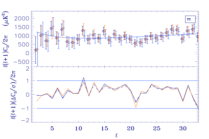
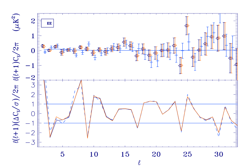
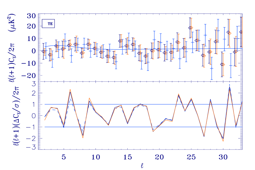
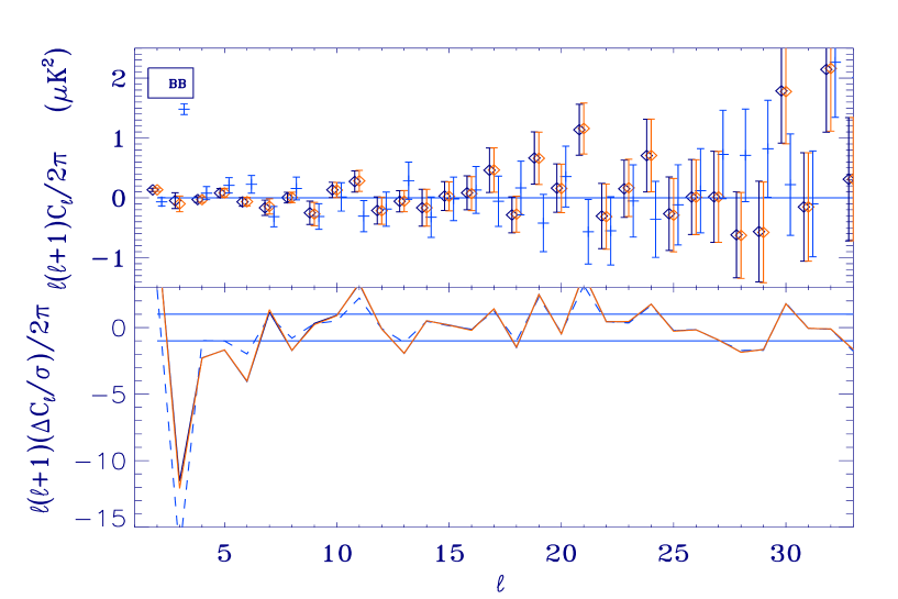
We present the results obtained by our implementation of the QML estimator on the low resolution WMAP5 maps described in the previous section and those obtained by the WMAP team in Figs. 1-4, respectively for TT, EE, TE and BB spectra. In the top panels we show the estimates of BolPol with error bars (dark blue or red, see below) and the (pseudo-$C_{\ell}$) estimates obtained by the WMAP team with error bars (light blue). The BolPol estimates in dark blue are obtained by using as fiducial spectrum the theoretical WMAP5 best-fit (Dunkley et al., 2009), a $\tau\Lambda$CDM cosmological model with $\Omega_{b}h^{2}=0.0227$, $\Omega_{c}h^{2}=0.108$, $H_{0}=72.4kms^{-1}Mpc^{-1}$, $\tau=0.089$, $n_{s}=0.961$, $A_{s}=2.41\times 10^{-9}$ (at $k=0.002Mpc^{-1}$). Error bars loose dependence on the fiducial model by iterating the QML: we use the first run of BolPol to obtain another set of estimates with relative error bar, which is plotted in red. The iterated estimates are always very close to those obtained with the WMAP5 best-fit as fiducial model: this means that the QML estimated are sufficiently stable with respect to iteration. The same does not happen to the error bars: in particular the error on the TT quadrupole is substantially smaller, and a decrease of the error also occurs for $\ell=3\,,4$ in temperature. Our estimate for the octupole in BB is consistent with zero and very different from the one obtained by WMAP (note however that the WMAP likelihood slice for $C^{BB}_{\ell=3}$ is not anomalous as the WMAP pseudo-$C_{\ell}$ estimate (Nolta et al., 2009)).

In the lower panels of Figs. 1-4 we show the differences between the sets of estimates in unit of sigma (same conventions as upper panels). More precisely we show $(C_{\ell}^{BolPol}-C_{\ell}^{WMAP})/\sigma$ where the BolPol estimates and $\sigma$ are given by: BolPol estimates with BolPol error bars for the no-iteration case (solid dark blue lines); BolPol estimates in the no-iteration case and WMAP error bars (dashed light blue line); BolPol estimates with BolPol error bars for the iteration case (solid red line). These lower plots show and quantify the differences among the considered sets of estimates. Our estimate of the TT spectrum is within 1$\sigma$ from the one computed by the WMAP team. For the other spectra we find larger differences (even 2$\sigma$). The current joint analysis is very different from the one performed by the WMAP team and it is obvious to expect larger differences for the more delicate spectra (where the Signal to Noise ratio is lower).

We list now the reduced $\chi^{2}$ values for the iterated BolPol estimates from $\ell=2$ to $\ell=32$ with the fiducial input model: $\chi^{2}_{TT}=4.423$ but excluding the quadrupole this value decreases to $1.079$ recovering so the anomaly of the low quadrupole value of TT; for the other reduced $\chi^{2}$-values we find $\chi^{2}_{TE}=0.785$, $\chi^{2}_{EE}=1.422$, $\chi^{2}_{BB}=1.607$.

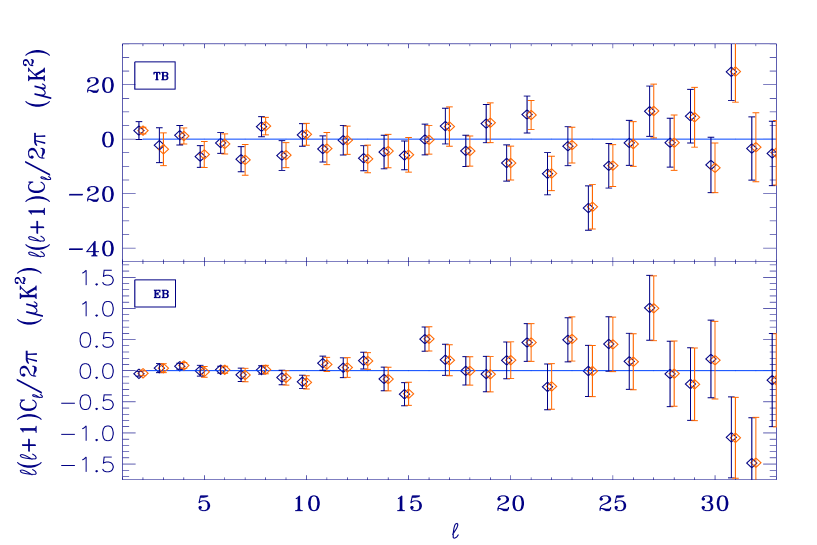
In Fig. 5, we plot the first and iterated BolPol estimates and relative error bars (in blue and red, respectively) for TB and EB. We do not plot the estimates by the WMAP team since these are not provided in the LAMBDA site. Also for these parity-odd correlators the QML estimates are very stable with respect to the iteration. Note how the error bars in TB change (due to substantially different fiducial model in TT in the iterated run), whereas those in EB do not (since the fiducial EE and BB spectra are mainly unchanged during the iteration). The TB null reduced $\chi^{2}$ for $\ell=2-23$ is $1.34$ to be compared with $0.97$ quoted for $\ell=24-450$ by the WMAP team. The EB null reduced $\chi^{2}$ for $\ell=2-23$ is $1.14$.

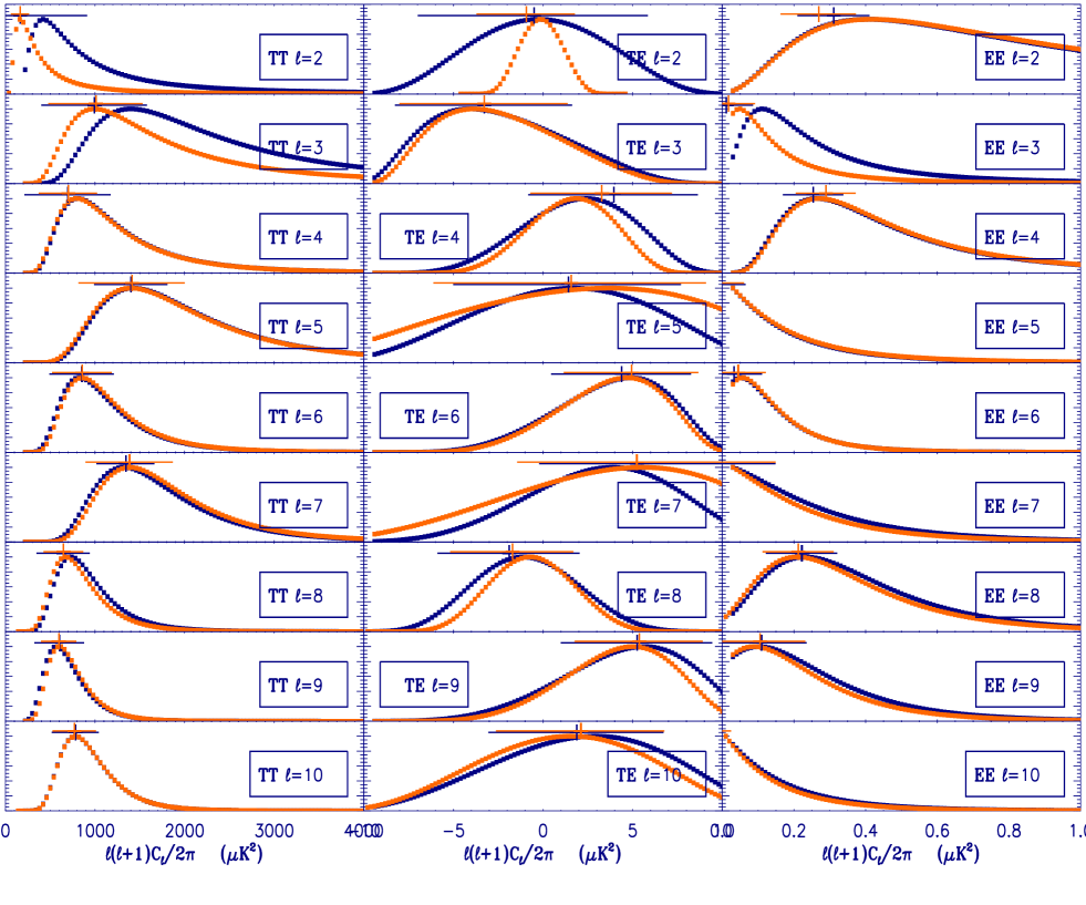
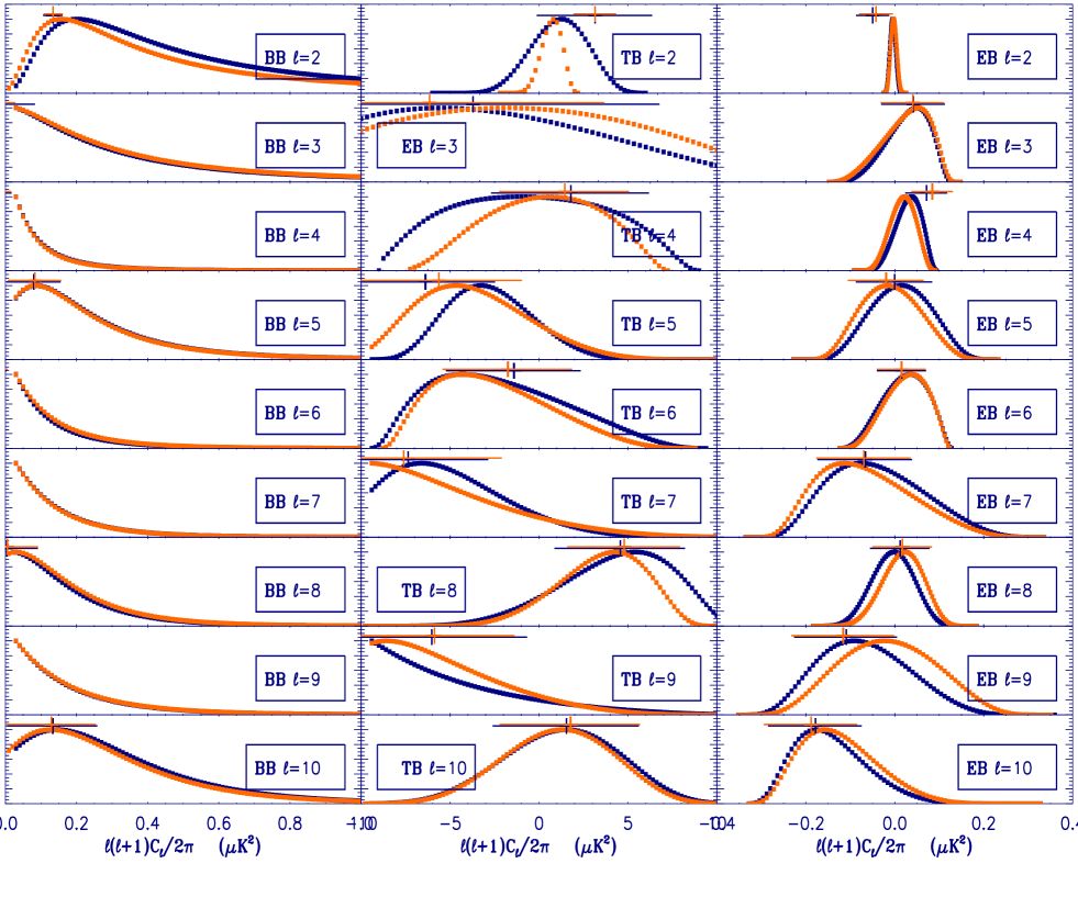
At low multipoles, symmetric error bars, such as those provided by the Fisher matrix, are just an approximation, since we know that the likelihood for $C_{\ell}$ is far from a symmetric Gaussian. We therefore evaluate the conditional likelihood slices for the six spectra from $\ell=2$ to $10$; we present these results in Figs. 6-7. As for the QML, we compute the slices on the WMAP5 best-fit (blue points) and on the BolPol estimates (orange points obtained with the same fiducial used for the iterated QML run). It is important to note that the peaks of the likelihood slices are very different for the two sets of conditionings: the quadrupole in temperature is the most striking example. We do not observe such dependence on the fiducial model in the estimates in the QML method. As for the errors of the QML method, also the shape of the conditional slices depend on the fiducial model. The trend in the iteration is the same of the one observed for the QML: confidence levels shrink by inserting the iterated QML estimate as conditioning. In Figs. 6-7 we also plot the QML estimate with error bars as reference (blue plus for the first BolPol run and orange for the iterated one). The peaks of the likelihood slices are always consistent with the QML estimates within the error bars for both conditioning: however, an excellent agreement emerges when the QML estimates are used as conditioning.

Few results deserve to be commented for their cosmological importance. Our estimate (position of the peak) for the $\ell(\ell+1)C_{\ell}^{TT}/(2\pi)|_{\ell=2}$ is $165\,\mu K^{2}$ for the iterated QML (pixel base likelihood code). Basing on our pixel likelihood code, the conditional likelihood (normalized to 1) for $\ell(\ell+1)C_{\ell}^{TT}/(2\pi)|_{\ell=2}$ is larger than $0.05$ between $50\,\mu K^{2}$ and $1305\,\mu K^{2}$. This last value has to be compared with the one given in Fig. 1 of Dunkley et al. (2009), in which we read that $\ell(\ell+1)C_{\ell}^{TT}/(2\pi)|_{\ell=2}$ is approximatively less than $1600\,\mu K^{2}$ at the same confidence level.

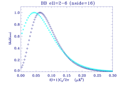
We also obtain constraints on $BB$. In Fig. 8 we show the conditional likelihood slice for the band powers, $\ell(\ell+1)C_{\ell}^{BB}/(2\pi)$ binning from $\ell=2$ to $6$. Dark blue diamonds of Fig. 8 represent the likelihood slice we obtain sampling on band powers. We find $\ell(\ell+1)\,C_{\ell}^{BB}/(2\pi)|_{2-6}<0.18\mu K^{2}$ at $95\%$ of C.L. (this bound decreases to $0.13\mu K^{2}$ at $95\%$ of C.L. averaging over $\ell=2-10$). Light blue crosses in Fig. 8 represent the conditional likelihood slice we obtain sampling on $C_{\ell}$. In this case we find $\ell(\ell+1)\,C_{\ell}^{BB}/(2\pi)|_{2-6}<0.19\mu K^{2}$ at $95\%$ of C.L. (this bound decreases to $0.11\,\mu K^{2}$ at $95\%$ of C.L. averaging over $\ell=2-10$). Some comments are in order: whereas it is expected to obtain different results sampling on different quantities, one may tentatively interpret the sampling on band powers more similar to a nearly scale-invariant spectrum of gravitational waves and the one on $C_{\ell}^{BB}$ similar to residual constant noise bias or a systematic. Whereas we do not find evidence for a $BB$ signal one may wonder about the different shapes of the conditional likelihood slices shown in Fig. 8: as a matter of fact, the quadrupole is the single multipole which contributes more to this discrepancy (see also the conditional likelihood slice for $C_{2}^{BB}$ in Fig. 7. Excluding the quadrupole from the analysis, the conditional likelihood slice sampled on band powers yields an upper limit of $\ell(\ell+1)\,C_{\ell}^{BB}/(2\pi)|_{3-6}<0.13\mu\,K^{2}$ at $95\%$ CL. While discrepancy is not statistically significant, the fact that it is mainly due to a single multipole might be ponting at a residual contamination in the WMAP 5 years map mostly affecting the quadrupole.

Figure 8: Upper bounds on BB. $y$ axis: Likelihood slice for BB. $x$ axis $\ell(\ell+1)C_{\ell}^{BB}/(2\pi)$ binning from $\ell=2$ to $6$. Dark blue diamonds represent the likelihood slice obtained sampling on band powers. Light blue crosses represent the likelihood slice obtained sampling on power spectrum. See also the text.

6 Discussions and Conclusions

We have performed a new estimate of the CMB angular power spectra at low multipoles from low resolution maps of the five years WMAP data.

The QML estimates are found in agreement with the pseudo-$C_{\ell}$ WMAP ones: the best agreement is for the TT spectrum and differences at the level of $2-3\,\sigma$ are found in EE and BB.

Whereas the QML is not used by the WMAP team, a pixel likelihood code is employed and results are given in Dunkley et al. (2009), Nolta et al. (2009). The difference between the conditional likelihood slices given here and those obtained by the WMAP team are due to our exact treatment of the covariance matrix: the approximation used by the WMAP team requires less computational resources but has the drawback of allowing negative values for conditional slices of EE and BB whereas ours are always positive. The origin of the difference in the constraint in $C_{\ell}^{BB}$ for $\ell=2-6$ is partially due to this difference.

References

- Benabed et al. (2009) Benabed K., Cardoso J. F., Prunet S. and Hivon E., arXiv:0901.4537 [astro-ph.CO].
- Bond, Jaffe and Knox (1998) Bond J. R., Jaffe A. H. and Knox L., Phys. Rev. D 57, 2117 (1998) [arXiv:astro-ph/9708203].
- Chu et al. (2005) Chu M., Eriksen H. K., Knox L., Górski K. M., Jewell J. B., Larson D. L., O’Dwyer I. J., Wandelt B. D., 2005, PhRvD, 71, 103002
- Dickinson et al. (2007) Dickinson C., Eriksen H. K., Jewell J., Banday A. J., Gorski K. M., Lawrence C. R., 2007, AAS, 38, 883
- Dunkley et al. (2009) Dunkley J. et al. (WMAP), apj SS 180 (2009) 306, arXiv:0803.0586 [astro-ph].
- Efstathiou (2004) Efstathiou G., Mon. Not. Roy. Astron. Soc. 348, 885 (2004)
- Efstathiou (2004) Efstathiou G., Mon. Not. Roy. Astron. Soc. 349, 603 (2004) [arXiv:astro-ph/0307515].
- Eriksen et al. (2004) Eriksen H. K. et al., Astrophys. J. Suppl. 155, 227 (2004) [arXiv:astro-ph/0407028].
- Eriksen et al. (2007) Eriksen H. K., Huey G., Banday A. J., Górski K. M., Jewell J. B., O’Dwyer I. J., Wandelt B. D., 2007, ApJ, 665, L1
- Friedman et al. (2009) Friedman R. B. et al. [QUaD collaboration], arXiv:0901.4334 [astro-ph.CO].
- Gorski et al. (2005) Gorski K.M., Hivon E., Banday A.J., Wandelt B.D., Hansen F.K., Reinecke M. and Bartelmann M., 2005, HEALPix: A Framework for High-resolution Discretization and Fast Analysis of Data Distributed on the Sphere, Ap.J., 622, 759-771
- Grain et al. (2009) Grain J., Tristram M. and Stompor R., arXiv:0903.2350 [astro-ph.CO].
- Hauser and Peebles (1974) Hauser, M. G.; Peebles, P. J. E., Astrophysical Journal, Vol. 185, pp. 757-786 (1973)
- Hinshaw et al. (2003) Hinshaw G. et al. [WMAP Collaboration], Astrophys. J. Suppl. 148, 135 (2003) [arXiv:astro-ph/0302217].
- Hinshaw et al. (2007) Hinshaw G. et al. [WMAP Collaboration], Astrophys. J. Suppl. 170, 288 (2007) [arXiv:astro-ph/0603451].
- Hivon et al (2002) Hivon E. et al., Astrophys. J. 567, 2 (2002)
- Jewell et al. (2004) Jewell J., Levin S. and Anderson C. H., Astrophys. J. 609, 1 (2004) [arXiv:astro-ph/0209560].
- Jones et al. (2006) Jones W. C. et al., Astrophys. J. 647, 823 (2006) [arXiv:astro-ph/0507494].
- Kogut et al. (2003) Kogut A. et al. [WMAP Collaboration], Astrophys. J. Suppl. 148, 161 (2003) [arXiv:astro-ph/0302213].
- Kuo et al (2004) Kuo C. I. et al. [ACBAR collaboration], Astrophys. J. 600, 32 (2004) [arXiv:astro-ph/0212289].
- Larson et al. (2007) Larson D. L., Eriksen H. K., Wandelt B. D., Górski K. M., Huey G., Jewell J. B., O’Dwyer I. J., 2007, ApJ, 656, 653
- Montroy et al. (2006) Montroy T. E. et al., Astrophys. J. 647, 813 (2006) [arXiv:astro-ph/0507514].
- Nolta et al. (2009) Nolta J. et al. (WMAP), apj SS 180 (2009) 296, arXiv:0803.0593 [astro-ph].
- Page et al. (2007) Page L. et al. [WMAP Collaboration], Astrophys. J. Suppl. 170, 335 (2007) [arXiv:astro-ph/0603450].
- Pearson et al. (2003) Pearson T. J. et al., Astrophys. J. 591, 556 (2003) [arXiv:astro-ph/0205388].
- Piacentini et al. (2006) Piacentini F. et al., Astrophys. J. 647, 833 (2006) [arXiv:astro-ph/0507507].
- Polenta et al. (2005) Polenta G. et al., JCAP 0511, 001 (2005) [arXiv:astro-ph/0402428].
- Pryke et al. (2008) Pryke C. et al. [QUaD collaboration], arXiv:0805.1944 [astro-ph].
- Rudjord et al. (2009) Rudjord Ø., Groeneboom N. E., Eriksen H. K., Huey G., Górski K. M., Jewell J. B., 2009, ApJ, 692, 1669
- Saha et al. (2006) Saha R., Jain P. and Souradeep T., Astrophys. J. 645, L89 (2006) [arXiv:astro-ph/0508383].
- Taylor et al. (2007) Taylor J. F., Ashdown M. A. J. and Hobson M. P., arXiv:0708.2989 [astro-ph].
- Tegmark (1997) Tegmark M., Phys. Rev. D 55, 5895 (1997)
- Tegmark and de Oliveira-Costa (2001) Tegmark M. and de Oliveira-Costa A., Phys. Rev. D 64 (2001) 063001
- Wandelt et al. (2004) Wandelt B. D., Larson D. L. and Lakshminarayanan A., Phys. Rev. D 70, 083511 (2004) [arXiv:astro-ph/0310080].
- Wu et al. (2007) Wu J. H. et al., Astrophys. J. 665, 55 (2007) [arXiv:astro-ph/0611392].
- Wu et al. (2008) Wu E. Y. et al. [QUaD Collaboration], arXiv:0811.0618 [astro-ph].