A Bayesian approach to the analysis of time symmetry in light curves:
Reconsidering Scorpius X-1 occultations

Abstract

We present a new approach to the analysis of time symmetry in light curves, such as those in the x-ray at the center of the Scorpius X-1 occultation debate. Our method uses a new parameterization for such events (the bilogistic event profile) and provides a clear, physically relevant characterization of each event’s key features. We also demonstrate a Markov Chain Monte Carlo algorithm to carry out this analysis, including a novel independence chain configuration for the estimation of each event’s location in the light curve. These tools are applied to the Scorpius X-1 light curves presented in Chang et al. (2007), providing additional evidence based on the time series that the events detected thus far are most likely not occultations by TNOs.

1. Introduction

As new surveys accumulate vast databases of astronomical light curves (Hodapp et al. 2004; Starr et al. 2002), the identification and analysis of events in these time series is becoming an increasingly important task (e.g. Preston et al. (2009); Stewart (2009)). One of the topics of such analyses is examining the symmetry of such events. Traditionally, symmetry has been analyzed by examining the skewness of each event, sometimes after stacking the light curves (for examples, see Jones et al. (2006, 2008)). However, this approach is not satisfactory for x-ray light curves due to the small number of counts involved, particularly during suspected occultation events. Additionally, the nonparametric approach of examining skewness has significantly lower power than a parametric analysis with a well parameterized model, especially considering the large mean squared errors of common skewness estimators (see Joanes & Gill (1998)). This means that, for a given false-positive rate, a well-designed parametric analysis will have a lower false-negative rate than a nonparametric approach.

The debate over the nature of the observed Scorpius X-1 events has raged in the literature since 2006. It began with the publication of Chang et al. (2006), which claimed the detection of at least 58 occultations of Scorpius X-1 by small (diameter $<$ 100m) TNOs. The size distribution of these small TNOs bears important clues of the dynamical evolution of the early Solar System (e.g. Pan & Sari (2005); Kenyon & Bromley (2004)), yet the vast majority of TNO population is still way beyond the limit of direct observation by even the largest ground-based telescopes. Occultation of background stars by TNOs is the only present observational method able to reach the smaller objects (Bailey 1976; Lehner et al. 2008; Roques et al. 2006; Bickerton et al. 2008; Bianco et al. 2009). This finding was challenged later that year by Jones et al. (2006). The latter group claimed that the observed events were unlikely to be occultations by TNOs because the stacked profile for these events was asymmetric. However, this analysis was not entirely satisfactory from a statistical perspective; it was performed on heavily transformed versions of the originally data, did not take into account the discrete nature of the observations, and provided no measures of uncertainty.

The response of Chang et al. to this analysis was Chang et al. (2007), wherein they claimed to have identified 12 events in the Scorpius X-1 data that were unlikely to have originated from instrumental effects. However, this claim was challenged again by Jones et al. (2008). Jones et al. presented evidence that the observed events were due to charged particle events in the detectors. Their argument relied again, in part, on the claim that the observed event were not temporally symmetric. Unfortunately, their analysis had not proceeded beyond a simple stacking-based approach (analogous to Jones et al. (2006)), so the validity of these conclusions remains uncertain.

Most recently, Liu et al. (2008) presented a new analysis of 72-ks of data of Sco-X1 taken in the year 2007. Liu et al. concluded that no significant dips which might be real occultation by $60-100$ m TNOs were observed.

In this paper we introduce a new parameterization for unimodal events in light curves, called the bilogistic event profile. This parameterization can describe a wide range of possible events and naturally yields estimates of physically interesting quantities such as the full width at half maximum (FWHM) of the event. Additionally, our parameterization can be applied in both the Poisson and Gaussian regimes.

Additionally, we demonstrate a computational approach to inference with the bilogistic event profile using Markov chain Monte Carlo (MCMC) methods. This includes the introduction of a novel approach to the construction of a proposal distribution for the center of the event, improving the efficiency of our simulations.

Finally, we apply our parameterization and computational approach to occultation events identified in the Scorpius X-1 RXTE data in Chang et al. (2006) and Chang et al. (2007). Our analysis lends further support to the argument that the events identified thus far are instrumental in origin, as suggested in Jones et al. (2006) and Jones et al. (2008).

In § 2, we describe the details of our data model for the Scorpius X-1. We present the details of our MCMC approach in § 3. The results of applying our method to simulated data are discussed in § 4. Our primary scientific results on the Scorpius X-1 light curves comprise § 5. We conclude in § 6.

2. Model

2.1. Context & Specification

We have a time series of counts $\{y_{t}\}$, $t\in\{0,\cdots,T-1\}$. We assume that each count is distributed as an independent Poisson random variable, conditional on the source intensity at time $t$:

$$y_{t}\sim Poisson(\lambda_{t}).$$

We also believe that an event of some kind has occurred in this time series. For the sake of this discussion, we assume that this event is characterized by a dimming of the source (e.g., a transit). However, this framework can be extended trivially to events character by increased intensity (e.g., supernovae) or the high-count regime (with a Gaussian distribution replacing the Poisson). The key constraint is that we know a priori the sign of the expected deviation from the baseline intensity. We characterize the intensity $\lambda_{t}$ as

$$\lambda_{t} =c-\alpha\,g(t;\tau,\overrightarrow{\theta})$$

where $\lim_{t\rightarrow\infty}g(t;\tau,\overrightarrow{\theta})=\lim_{t\rightarrow-\infty}g(t;\tau,\overrightarrow{\theta})=0$ and $\sup_{\mathbb{R}}g(t;\tau,\overrightarrow{\theta})=g(\tau;\tau,\overrightarrow{\theta})=1$. We will call $g(t;\tau,\overrightarrow{\theta})$ the event profile, as it characterizes the pattern of intensity changes throughout the event. The parameter $\tau$ is the time index about which the event is hypothesized to be time-symmetric, and $\overrightarrow{\theta}$ is a vector of parameters characterizing the event. $c$ sets the baseline intensity of the source, and $\alpha$ sets the peak size of the deviation from the baseline intensity during the event. All of these parameters must be estimated from the data.

Putting all of these points together with the log-likelihood for the model, we obtain:

$$\ell(c,\alpha,\tau,\overrightarrow{\theta};\overrightarrow{y}) =\sum_{t=0}^{T-1}[y_{t}\ln{(\lambda_{t})}-\lambda_{t}]+\rm{const}$$ (1)

Following Bayesian approach we can express the posterior probability as a function of the likelihood and the prior probabilities as:

$$p(c,\alpha,\tau,\overrightarrow{\theta}\mid\overrightarrow{y}) \propto\ell(c,\alpha,\tau,\overrightarrow{\theta};\overrightarrow{y})\times p(c,\alpha,\tau,\overrightarrow{\theta})$$ (2)

Having obtained the posterior of our parameters (up to a normalizing constant), we have all of the information needed to make inferences about the parameters of interest. We can characterize our inferences about the locations of parameters via their posterior means and medians. Our uncertainty about these parameters can be characterized by $68\%$ posterior intervals or posterior standard deviations. However, it still remains to specify a functional form for the event profile $g(t;\tau,\overrightarrow{\theta})$.

2.2. Bilogistic event profile

The choice of event profile $g(t;\tau,\overrightarrow{\theta})$ is quite important to this analysis. One must achieve the proper balance between parsimony in parameterization and giving the model enough flexibility to fit a wide range of event shapes. To that end, we introduce the bilogistic event profile:

$$g(t;\tau,h_{1},h_{2},k_{1},k_{2})=\frac{1+e^{\frac{-h_{t}}{k_{t}}}}{1+e^{\frac{|t-\tau|-h_{t}}{k_{t}}}}$$ (3)

$$h_{t}=\left\{\begin{array}[]{l l}h_{1}&t<\tau\\ h_{2}&t\geq\tau\end{array}\right.$$ (6)

$$k_{t}=\left\{\begin{array}[]{l l}k_{1}&t<\tau\\ k_{2}&t\geq\tau\end{array}\right.$$ (9)

This event profile is characterized by four parameters (in addition to the location parameter $\tau$). The first two parameters ($h_{1}$ and $h_{2}$) characterize the (approximate) half-maxima of the event’s amplitude, represented as deviations from the event’s center; we will refer to them as the “half-life” parameters. This holds only approximately because of the correction for continuity in the numerator (the $e^{\frac{-h_{t}}{k_{t}}}$ term), which ensures that the event profile is continuous at time $\tau$. Thus, $(h_{1}-h_{2})$ characterizes the departure of our event from symmetry in terms of the half-maxima, and $(h_{1}+h_{2})$ characterize the (approximate) full width at half maximum for our event.

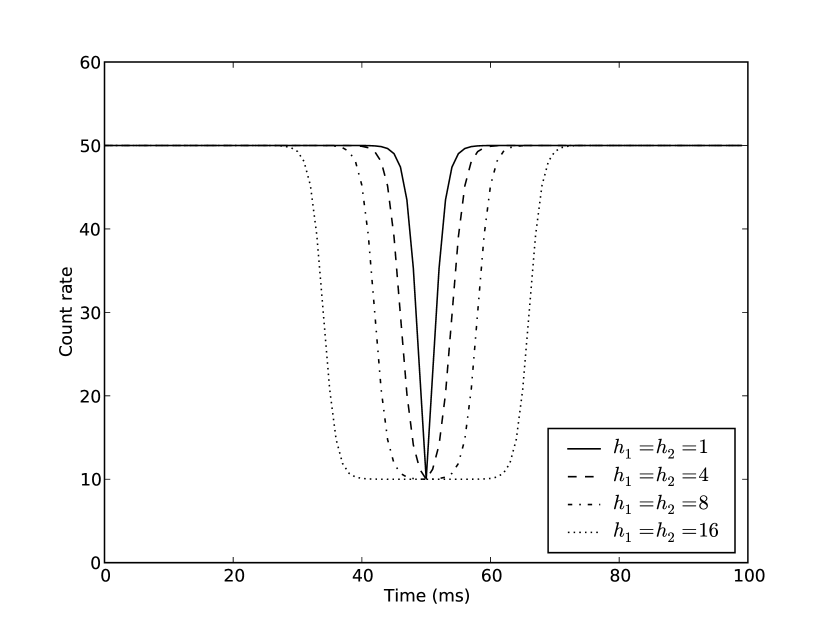
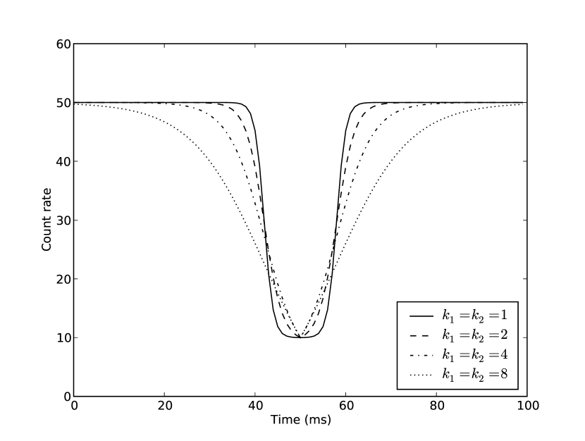
The second set of parameters ($k_{1}$ and $k_{2}$) characterize the rate at which the intensity changes during our event; we will refer to them as the “curvature” parameters. The first ($k_{1}$) characterizes how rapidly our source’s intensity diminishes at the beginning of our event, and the second characterizes how rapidly the intensity returns to the baseline at the end of our event. If $k_{1}<<h_{1}$ and $k_{2}<<h_{2}$, as is often the case, the curvature parameters can been viewed as pivoting our event profile through the half-intensity points set by $h_{1}$ and $h_{2}$, with higher values corresponding to sharper changes in intensity. These features of the bilogistic event profile can be seen in Figures 1 and 2, where we fix one set of parameters ($h_{1}$ and $h_{2}$ or $k_{1}$ and $k_{2}$) and vary the other.

To perform inference using this model, we first consider it in a Bayesian light, assuming flat priors on all parameters except $\tau$. We place one restriction on $\tau$ a priori. We assume that the event is centered within the interior of our light curve. In this context, we take interior to mean far enough from the boundaries that the event is contained within our light curve. This assumption is reasonable for our analysis because the light curves we are working with have been extracted and preprocessed to contain one complete event each. Thus, we impose a prior probability of zero on values of $\tau$ within $m$ milliseconds of the edge of the light curve for our analysis; for the analysis presented here, we set $m=10$ milliseconds. This assumption also improves the computational properties of our posterior simulations by preventing them from becoming “stuck” at values of the $\tau$ parameter that are near the ends of the light curve. The end result of these restrictions is that our prior on $\tau$ is uniform on the set $[m,T-m]$.

We can then use a Markov chain Monte Carlo (MCMC) technique (the Metropolis-Hastings algorithm) to draw from the posterior distribution of our parameters. From these draws, we can calculate quantities such as the posterior median and 68% posterior intervals for $(h_{1}-h_{2})$ and $(k_{1}-k_{2})$ to characterize the deviation of our events from symmetry and our uncertainty about these properties. For an excellent introduction to the use of the Metropolis-Hastings algorithm for statistical inference, please consult Chib & Greenberg (1995).

3. Computational details of posterior simulations

Although the model presented above is quite appealing, the resulting posterior distribution for our parameters of interest is not analytically tractable. Thus, to make inferences about these parameters, we simulate a series of samples from their joint posterior distribution. We use a blocked Metropolis-Hastings algorithm for these simulations. This means that, instead of drawing new values for all seven of our parameters at once and accepting or rejecting them based on the Metropolis-Hastings rule, we vary only a subset of the parameters at time, holding all others fixed. The blocks used are: (1) $\tau$, (2) $c$ and $\alpha$, and (3) $h_{1}$, $h_{2}$, $k_{1}$ and $k_{2}$. So, for each iteration of our algorithm, we first draw a new value of $\tau$ from our proposal distribution and choose whether to accept it based on the Metropolis-Hastings acceptance probability. This acceptance probability is calculated holding the values of all other parameters ($c$, $\alpha$, $h_{1}$, $h_{2}$, etc.) fixed. Next, we draw new values of $c$ and $\alpha$ from our proposal distribution for these parameters and calculate an analogous acceptance probability. Finally, we perform a similar procedure on the shape parameters ($h_{1},h_{2},k_{1}$, and $k_{2}$). Blocking in this way allows us to take advantage of the structure in the model in constructing our simulation algorithm, improving its efficiency. For more information on blocked Metropolis-Hastings methods, please consult §6.2 of Chib & Greenberg (1995).

3.1. Initialization

We look to the data to obtain starting values for our MCMC algorithm. The first step is to obtain a smoothed version of our signal $y_{t}$, which we will denote $\tilde{y}_{t}$. This is generated by taking a centered moving average of the original signal $y_{t}$. For the analyses presented here, a window ten milliseconds wide was used, although this can be modified. The important point on the selection of the window is that it should be narrow enough to localize the event while still performing some noise reduction. If the window is too wide, our smoothed light curve will not capture the structure of the the event; as a result, it would not be useful in determining initial values for the magnitude ($\alpha$) or in determing the location of the event in the light curve. However, if the window is too narrow, it will not smooth the light curve well. As a result, our initializations would be far noisier than necessary.

Using $\tilde{y}_{t}$, we can construct our initialization values and a proposal distribution for $\tau$. Focusing on initialization first, we set $c_{0}=\operatorname{median}{(\tilde{y}_{t})}$ and $\alpha_{0}=c_{0}-\min_{t}(y_{t})$. We use a robust measure of typical baseline rate (the median). The motivation for this initialization of c is that, if the event is brief relative to the duration of the light curve and our smoothing window is not too long, our smoothed light curve should be near the baseline count rate $c$ for most times. In contrast, if we simply used the overall mean, it would be contaminated by the event of interest. Our initialization for $\alpha$ is relatively straightforward; we take our estimate of the baseline rate ($c_{0}$) and subtract the minimum observed count rate to obtain an estimate of the magnitude of our event.

To initialize $h_{1}$ and $h_{2}$, we take a similar approach. First, we assume that a symmetric initialization will be an acceptable starting point for our analysis. We then calculate $h_{0}=\frac{1}{2}\#\left\{t:y_{t}<\frac{\operatorname{median}{(\tilde{y}_{t})}+\min_{t}(y_{t})}{2}\right\}$ and set $h_{1}$ and $h_{2}$ to $h_{0}$. Based on the above discussion of $c_{0}$ and $\alpha_{0}$, this approach to initializing $h_{1}$ and $h_{2}$ appears quite natural. We are using our initial estimates of $c$ and $\alpha$ to estimate the FWHM of our event and attributing equal parts of this time to $h_{1}$ and $h_{2}$. Finally, we initialize $k_{1}$ and $k_{2}$ manually. Our posterior simulations were quite insensitive to the initializations of these parameters; values between 1 and 20 yielded similar results.

3.2. Metropolis-Hastings steps

Keeping in mind the prior discussed in §2.2, we can obtain a proposal distribution for $\tau$ using the procedure outlined in Algorithm 1.

Algorithm 1 Construction of proposal distribution for $\tau$

0:  $\tilde{y}_{t}$ for $t\in\{1,\ldots,T\}$, $m\in\mathbb{N}$, $p>0$, $\epsilon>0$

  $\tilde{w}_{t}\leftarrow(\max_{t}{(\tilde{y}_{t})}-\tilde{y}_{t})^{p}$

  $\tilde{w}_{t}\leftarrow\tilde{w}_{t}+\epsilon$

  if $t<m$ or $(T-t)<m$ then

     $\tilde{w}_{t}\leftarrow 0$

  end if

  $w_{t}\leftarrow\frac{\tilde{w}_{t}}{\sum_{t}\tilde{w}_{t}}$

  Calculate points along cumulative distribution function (CDF) as $p_{t}=\sum_{s\leq t}w_{s}$

  Calculate CDF $F(t)$ via linear interpolation of $\{p_{t}\}$

  Calculate quantile function $q(p)$ via linear interpolation

  Calculate density function $f(t)$ as derivative of $F(t)$ for $t\notin\mathbb{N}$

At the conclusion of this procedure, we have the density, cumulative density, and quantile functions for our proposal distribution for $\tau$. Through a series of numerical experiments, we found that values of $p$ between two and five typically produced the best proposal distributions; $p$ was set to four in the subsequent analyses. The $\epsilon$ term serves to ensure that all $w_{t}$ are non-zero, avoiding an issue with the interpolation of our quantile function (where a $w_{t}$ of zero leads to a vertical segment). We use linear interpolation because it is the only spline method that produces identical functions when the axes are exchanged. This is vital in our application because we are conducting seperate interpolations of $\{p_{t}\}$ to obtain our CDF and its inverse (the quantile function). If we had used any other type of polynomial interpolation, the inverse of the calculated spline for the CDF would not be another polynomial spline. However, with a linear spline, the inverse of the interpolated function is simply another linear spline. Thus, we can avoid complex calculations and use standard interpolation routines to calculate our quantile function. Our method of generating a proposal for our location parameter is quite versatile, adapting naturally to the presence of multiple potential events in the light curve. We will discuss some potential applications of it beyond this analysis in § 6.

The proposal generated by the above procedure allows us to use an independence chain Metropolis-Hastings method for $\tau$. With this class of methods, the proposal distribution for the parameter being simulated is independent of that parameter’s current value in the MCMC simulation. If the proposal is well-constructed, this can greatly improve the convergence properties of the simulations; in the ideal case, we would make our proposal the same as our posterior to maximize efficiency. However, for such a procedure to be effective, one must have some prior knowledge of the parameters’s posterior distribution. That is what the above procedure extracts from the light curve.

Using the initial values and proposal distribution obtained above, we construct proposal distributions for the parameters of our model (excepting $\tau$). All proposals are Gaussian and are thus characterized by their means and standard deviations:

$$(c,\alpha)\>: \;\mu=(c_{0},\alpha_{0}),\;\sigma=(\sqrt{\frac{c_{0}}{T}},\sqrt{\alpha_{0}})$$ (10)

$$(h_{1},h_{2})\>: \;\mu=(h_{1}^{i-1},h_{2}^{i-1}),\;\sigma=(\frac{\sqrt{h_{0}}}{2},\frac{\sqrt{h_{0}}}{2})$$ (11)

$$(k_{1},k_{2})\>: \;\mu=(k_{1}^{i-1},k_{2}^{i-1}),\;\sigma=(\frac{\sqrt{k_{0}}}{2},\frac{\sqrt{k_{0}}}{2})$$ (12)

With these proposals and the blocking scheme described previously, we have fully specified our MCMC simulation approach. We now demonstrate it’s effectiveness with simulated data.

4. Results on simulated symmetric events

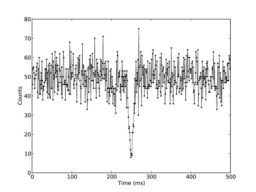
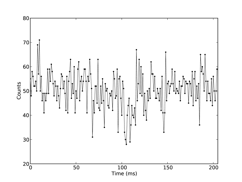
To test our approach, we simulated a 500 time steps light curve with a symmetric event resembling those observed in the Scorpius X-1 data. For this simulation, we set $c=50$, $\alpha=40$, $h_{1}=h_{2}=5$, $k_{1}=k_{2}=2$, and $\tau=300$. The resulting light curve can be seen in Figure 3.

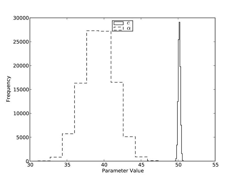
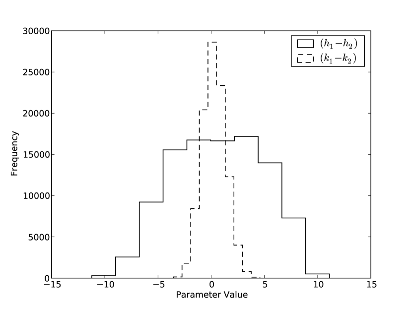
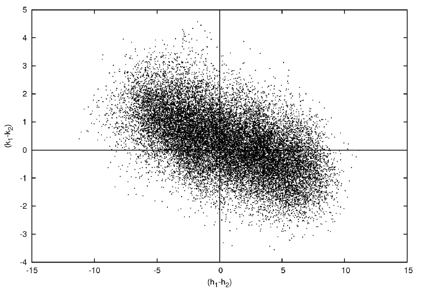
The results of the posterior simulations are summarized in Figure 4, Figure 5, and Figure 6. From the first of these (Figure 4), we observe that the posterior distributions for both the baseline count rate ($c$) and the magnitude of the event ($\alpha$) are centered around their true values of 50 and 40, respectively. The posterior on $c$ is significantly more concentrated than the posterior on $\alpha$, as we would expect; we can use nearly every point in the light curve to infer the value of $c$, but we can only use the points during the event to infer the value of $\alpha$. The posterior distributions of $(h_{1}-h_{2})$ and $(k_{1}-k_{2})$ are considerably more diffuse, as Figure 5 demonstrates. These posteriors are, however, centered near the true value of 0. The relationship between the posterior distributions of these two quantities can be seen from Figure 6. There appears to be a significant negative dependence between the two deviations.

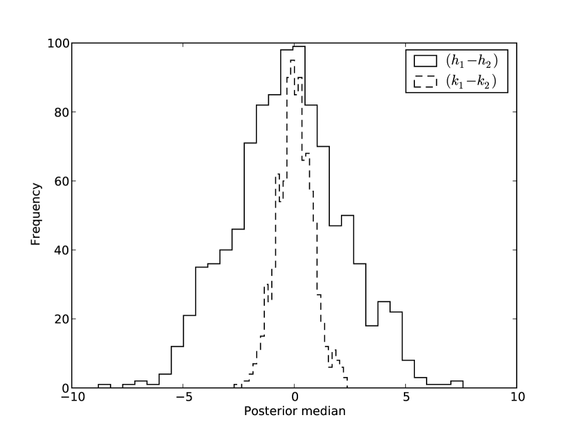
The properties of our estimates for symmetry-related parameters ($(h_{1}-h_{2})$ and $(k_{1}-k_{2})$) are further supported by a second set of simulations. Using the parameter values given above, we simulated 1000 light curves and ran our algorithm on each one. This allows us to quantify some frequentist properties of our Bayesian estimators, such as the coverage of our posterior intervals. The results of these simulations are summarized in Figure 7. Both distributions appear centered around zero. Coverage properties are not perfectly calibrated (as this is a Bayesian method), but they appear reasonable. 938 of our 1000 $68\%$ posterior intervals for $(h_{1}-h_{2})$ included zero, as did 816 of our $68\%$ posterior intervals for $(k_{1}-k_{2})$.

Overall, the results of this exercise with simulated events serve to increase our confidence in the validity of our method. We now apply our model and algorithm to the analysis of the Scorpius X-1 dip events.

5. Results on Scorpius X-1 events

Using the above model, we analyzed all 107 events from Chang et al. (2007). For each event, we ran our MCMC algorithm for $400,000$ iterations, discarding the first $200,000$ as burn-in. Run in parallel on Harvard’s Odyssey cluster, these runs required approximately 400 seconds in total (approximately $43,000$ CPU seconds). Typical acceptance rates for the individual Metropolis-Hastings steps were between 10% and 40%. The results of these simulations are summarized in Figure 8, Figure 9, and Figure 10.

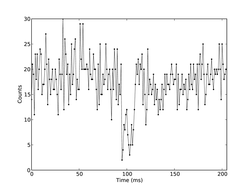
From Figure 8, we see that the FWHM of a typical event from Chang et al. (2007) is between 2 and 4 milliseconds (with $68\%$ posterior probability). Events 2 and 107 appears to be the only significant deviation from this pattern with FWHMs of approximately 7 and 13 milliseconds, respectively. Visual inspection of these events (in Figures 11 and 12) reveals that both are unusual in appearance. Event 2 is characterized by a more gradual change in intensity than most and appears to have two minimia. Event 107 appears to have two clear, significant minima.

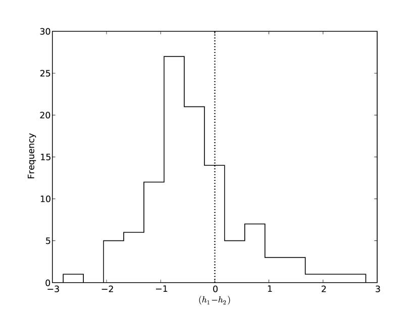
The posterior intervals for $(h_{1}-h_{2})$ in Figure 9 appear to be relatively evenly scattered around zero. However, although most of these intervals (90 of 107) cover zero, there is notable tendency towards negative values of $(h_{1}-h_{2})$. This can be seen in the posterior median, with 81 of the 107 posterior medians below zero. Using a classical sign test of the hypothesis that each posterior median is equally likely to be positive or negative (Dixon & Mood 1946), we obtain a p-value of $9.4\times 10^{-8}$, indicating that there is a significant deviation from symmetry in the relative half-maxima for this collection of events. The sign test is conducted by first counting the number of positive posterior medians. We then calculated the probability of observing a result at least as far from an even split of positive and negative medians as was observed, assuming that each median is equally likely to fall above or below zero. In this case, the p-value was calculated as $2\times P(X\leq 26|p=\frac{1}{2})$, where $X$ is the number of observed positive medians. Under the null hypothesis that positives and negatives are equally likely, $X\sim\mbox{Bin}(107,\frac{1}{2})$, so the preceding probability can be easily calculated using standard techniques for the binomial distribution. The pattern of negative deviations in $(k_{1}-k_{2})$ can also be seen in Figure 13; the deviation of this distribution from the symmetric case (seen in Figure 7) is clear. Events 2 and 107 appear somewhat anomalous in Figure 9; this is consistent with the unusual structure of these events discussed above.

Finally, the posterior medians for $(k_{1}-k_{2})$ are concentrated below zero (90 of 107 are negative). Inspection of the posterior intervals in Figure 10 indicates that very little posterior support is typically found above zero (only 55 of the 107 intervals included zero). A classical sign test on the posterior medians (as above) yields a p-value of $3.5\times 10^{-13}$. This indicates that the observed pattern of posterior medians is quite unlikely to occur if the true distribution of posterior medians is evenly distributed above and below zero. This is consistent with the findings of Liu et al. (2008), as a negative value of $(k_{1}-k_{2})$ indicates that the count rate decreased more quickly than it increased. The pattern of negative deviations in $(k_{1}-k_{2})$ can also be seen in Figure 14; the deviation of this distribution from the symmetric case (seen in Figure 7) is again apparent.

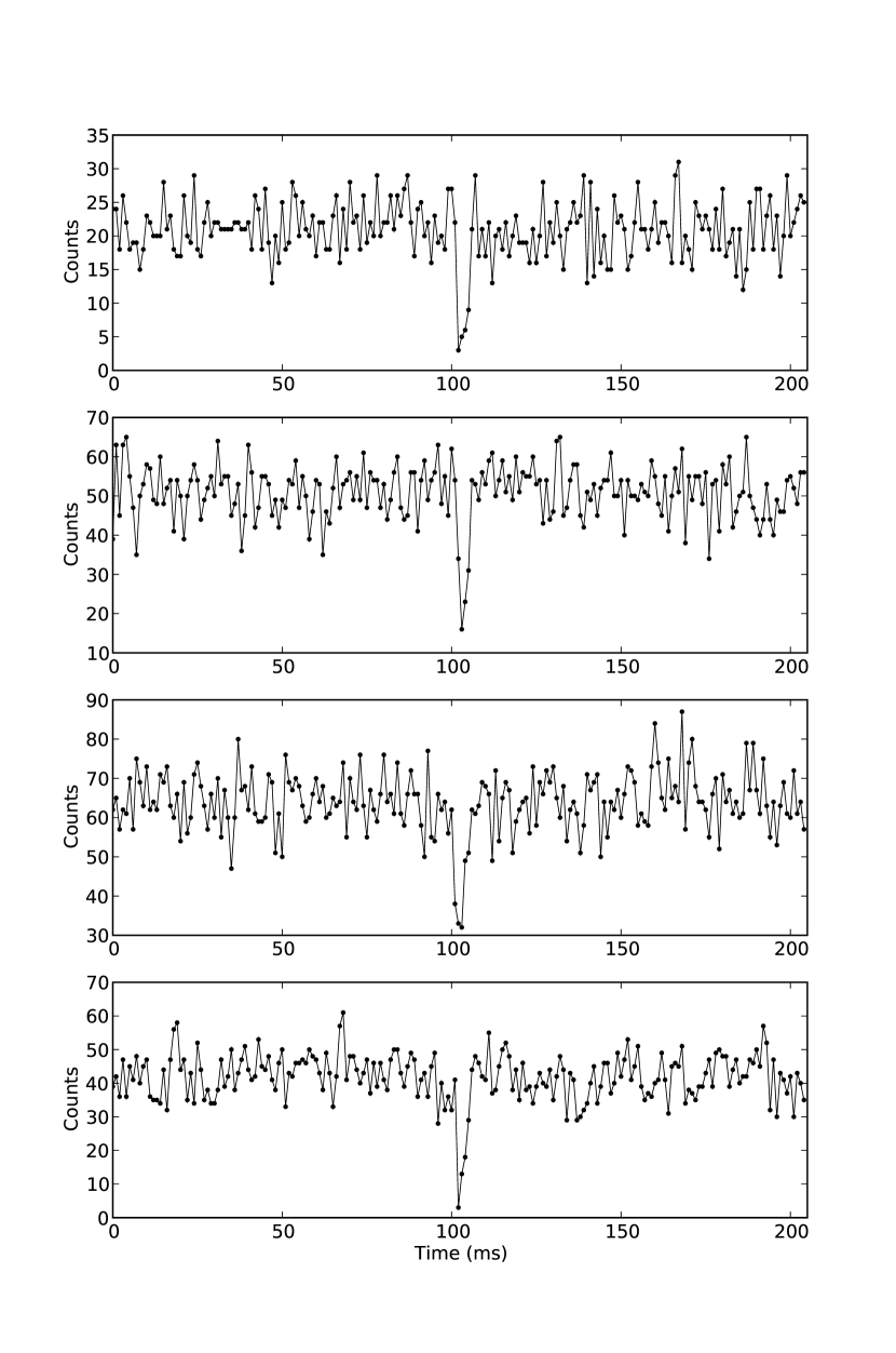
The concentration of $(h_{1}-h_{2})$ and $(k_{1}-k_{2})$ across events indicates that the observed events are characterized by a relatively rapid decrease in the count rate followed by a more gradual return to the baseline level; that is, the typical event profile is right-skewed. This pattern can be seen in Figure 15, which shows four representative events from Chang et al. (2007).

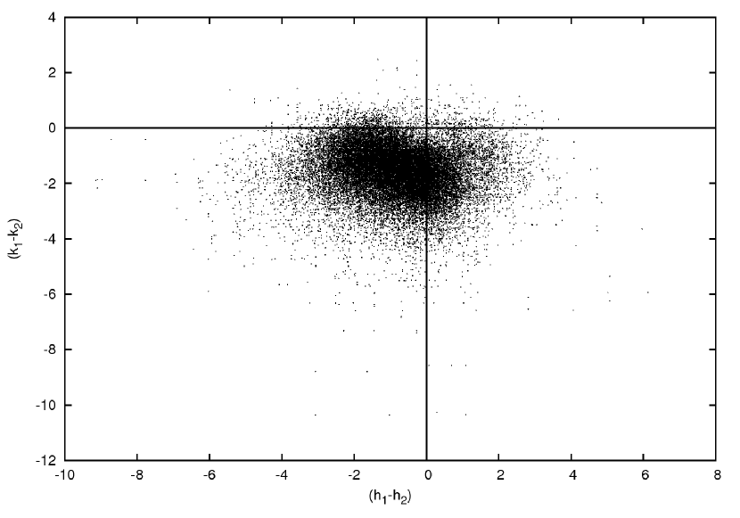
It is interesting to note that ($h_{1}-h_{2}$) and ($k_{1}-k_{2}$) are typically negatively correlated (when examining their joint posterior distribution) for approximately symmetric events. An example of this comes from our analysis of event 90 from Chang et al. (2007). The joint posterior distribution of ($h_{1}-h_{2}$) and ($k_{1}-k_{2}$) can be seen (as a scatterplot) in Figure 16. Two points are immediately apparent from this figure. First, the deviation of the distribution from the origin indicates that this event is most likely asymmetric. Second, ($h_{1}-h_{2}$) and ($k_{1}-k_{2}$) are strongly negatively correlated ($r=-0.618$). The intuition behind this outcome is clear. We are allowing for two possible deviations from symmetry in our model: deviations based on the half maxima ($h_{1}-h_{2}$) and deviations based on the rate of change ($k_{1}-k_{2}$) in our source’s intensity. For very short events, we cannot be certain to which of these deviations we should attribute the asymmetry of our event, as we can, to some extent, trade-off between them. Our posterior distribution simply reflects this trade-off.

It is also important to note that, when analyzed using our method, the events identified as potentially non-instrumental in origin by Chang et al. do not appear to deviate significantly from the remaining events in FWHM, half maxima deviation, or curvature deviation. This supports the conclusion of Liu et al. (2008) that the events detected thus far (including those identified as possibly non-instrumental) are most likely the result of dead-time effects and other instrumental contamination, not TNOs occulting Scorpius X-1.

At the distance of the Kuiper Belt ($\sim 40$AU) the size of the objects given the width of the events is $\sim 50$ m, and that is close to the Fresnel scale, which is $\sqrt{\lambda\;a/2}$, where $\lambda$ is the wavelength and $d$ is the distance. We use $\lambda=0.3$ nm (4 keV) because most of the RXTE/PCA-detected photons from Sco  X-1 are at this energy. As a result these occultation events are diffraction dominated phenomena (see Roques et al. (1987) and Nihei et al. (2007)) and we expect that diffraction effects would produce small count rate increases on either side of the dips.

Also TNOs of this size are not expected to be spherically symmetric (Roques et al. 1987) and therefore the resulting occultation events in the light curves are not expected to be time symmetric. However for TNOs of the size of the Fresnel scale or smaller the shape of the object does not translate into asymmetry of the time series. Roques et al 1986 has studied light curves from different shaped TNOs and demonstrated that when the effective size of the TNOs is smaller than the Fresnel scale the resulting events in the light curve do not differ from the light curves signatures of regularly spherically shaped TNOs. The sizes of the 107 objects studied here are within the range of the Fresnel scale so some asymmetry on the light curves should be manifested. Figures 17 and 18 show the measures of asymmetry as a function of the size of the object for 57 of the 58 events from Chang et al. (2006). As can be seen from the figures there is no clear relation between the estimated size of an object and the level of asymmetry for its corresponding event. This provides further evidence that the observed dips in intensity do not correspond to TNO transit events, as Jones et al. (2008) suggest.

6. Conclusions

Based on our analysis of the suspected Scorpius X-1 occultation events, we conclude that there is significant evidence for temporal asymmetry in these events. This finding is consistent with the suggestion of Jones et al. (2008) that the observed dips in brightness are due to dead time effects. We also conclude that the events identified in Liu et al. (2008) as possibly noninstrumental in origin are most likely not occultations.

We also note that the approach presented herein can be applied (with minor modifications) to the study of events in nearly any light curve. Such studies need not be limited to examining the symmetry of events, as the parameterization of our bilogistic event profile and flexible Bayesian approach allow inference to be made on quantities such as full width at half maxima. For example, our approach could be extended to analysis of exoplanetary transits, supernovae, quasars or any other transient event.

Furthermore, the method we have presented for constructing a proposal distribution for the center of each event can be applied quite generally. Even when using a physically grounded model with parameters such as body size, angle of incidence, etc., one must account for uncertainties about the location of the event in the light curve when making inferences about the parameters of interest. This can be quite challenging using classical methods, and even MCMC methods do not offer an panacea. Our approach to constructing an independence chain proposal distribution for the location parameter in such models makes them quite a bit more tractable, especially in the case of multiple events.

Figure 1.— Bilogistic event profile for $c=50$, $\alpha=40$, $k_{1}=k_{2}=1$, and $\tau=50$. Varying $h_{1}$ and $h_{2}$ from $1$ to $16$.

Figure 2.— Bilogistic event profile for $c=50$, $\alpha=40$, $h_{1}=h_{2}=8$, and $\tau=50$. Varying $k_{1}$ and $k_{2}$ from $1$ to $8$.

Figure 3.— Simulated light curve for symmetric event

Figure 4.— Histogram of posterior distributions of $c$ and $\alpha$ for simulated event

Figure 5.— Histogram of key symmetry-related parameters for simulated event

Figure 6.— $(k_{1}-k_{2})$ vs. $(h_{1}-h_{2})$ for simulated event

Figure 7.— Distributions of posterior medians of $(k_{1}-k_{2})$ and $(h_{1}-h_{2})$ for 1000 simulated events

Figure 8.— 68% posterior Intervals & medians for FWHM $(h_{1}+h_{2})$ for Chang et al. (2007) occultation events. Second plot is zoomed.

Figure 9.— 68% posterior Intervals & medians for $(h_{1}-h_{2})$ for Chang et al. (2007) occultation events. Second plot is zoomed.

Figure 10.— 68% posterior Intervals & medians for $(k_{1}-k_{2})$ for Chang et al. (2007) occultation events. Second plot is zoomed.

Figure 11.— Light curve for event 2 from Chang et al. (2007).

Figure 12.— Light curve for event 107 from Chang et al. (2007).

Figure 13.— Histogram of posterior medians for $(h_{1}-h_{2})$ for Chang et al. (2007) occultation events.

Figure 14.— Histogram of posterior medians for $(k_{1}-k_{2})$ for Chang et al. (2007) occultation events.

Figure 15.— Events 4, 19, 41, and 66 from Chang et al. (2007)

Figure 16.— $(k_{1}-k_{2})$ vs. $(h_{1}-h_{2})$ for event 90 from Chang et al. (2007).

Figure 17.— $|h_{1}-h_{2}|$ vs. estimated diameter for 57 of the 58 events from Chang et al. (2006) (58th event omitted due to anomalous nature).

Figure 18.— $|k_{1}-k_{2}|$ vs. estimated diameter for 57 of the 58 events from Chang et al. (2006) (58th event omitted due to anomalous nature).

References

- Bailey (1976) Bailey, M. E. 1976, Nature, 259, 290
- Bianco et al. (2009) Bianco, F. B., Protopapas, P., McLeod, B. A., Alcock, C. R., Holman, M. J., & Lehner, M. J. 2009, ArXiv e-prints
- Bickerton et al. (2008) Bickerton, S. J., Kavelaars, J. J., & Welch, D. L. 2008, AJ, 135, 1039
- Chang et al. (2006) Chang, H., King, S., Liang, J., Wu, P., Lin, L., & Chiu, J. 2006, Nature, 442, 660
- Chang et al. (2007) Chang, H.-K., Liang, J.-S., Liu, C.-Y., & King, S.-K. 2007, MNRAS, 378, 1287
- Chib & Greenberg (1995) Chib, S., & Greenberg, E. 1995, 49, 327
- Dixon & Mood (1946) Dixon, W. J., & Mood, A. M. 1946, Journal of the American Statistical Association, 41, 557
- Hodapp et al. (2004) Hodapp, K. W., et al. 2004, Astronomische Nachrichten, 325, 636
- Joanes & Gill (1998) Joanes, D., & Gill, C. 1998, Journal of the Royal Statistical Society (Series D): The Statistician, 47, 183
- Jones et al. (2006) Jones, T. A., Levine, A. M., Morgan, E. H., & Rappaport, S. 2006, The Astronomer’s Telegram, 949, 1
- Jones et al. (2008) —. 2008, ApJ, 677, 1241
- Kenyon & Bromley (2004) Kenyon, S. J., & Bromley, B. C. 2004, AJ, 128, 1916
- Lehner et al. (2008) Lehner, M. J., Wen, C. ., Wang, J. ., Marshall, S. L., Schwamb, M. E., Zhang, Z. ., Bianco, F. B., Giammarco, J., Porrata, R., Alcock, C., Axelrod, T., Byun, Y. ., Chen, W. P., Cook, K. H., Dave, R., King, S. ., Lee, T., Lin, H. ., & Wang, S. . 2008, ArXiv e-prints
- Liu et al. (2008) Liu, C.-Y., Chang, H.-K., Liang, J.-S., & King, S.-K. 2008, MNRAS, 388, L44
- Nihei et al. (2007) Nihei, T. C., Lehner, M. J., Bianco, F. B., King, S.-K., Giammarco, J. M., & Alcock, C. 2007, AJ, 134, 1596
- Pan & Sari (2005) Pan, M., & Sari, R. 2005, Icarus, 173, 342
- Preston et al. (2009) Preston, D., Protopapas, P., & Brodley, C. 2009, ArXiv e-prints. To appear in SIAM International Conference on Data Mining
- Roques et al. (2006) Roques, F., Doressoundiram, A., Dhillon, V., Marsh, T., Bickerton, S., Kavelaars, J. J., Moncuquet, M., Auvergne, M., Belskaya, I., Chevreton, M., Colas, F., Fernandez, A., Fitzsimmons, A., Lecacheux, J., Mousis, O., Pau, S., Peixinho, N., & Tozzi, G. P. 2006, AJ, 132, 819
- Roques et al. (1987) Roques, F., Moncuquet, M., & Sicardy, B. 1987, AJ, 93, 1549
- Starr et al. (2002) Starr, B. M., et al. 2002, in Society of Photo-Optical Instrumentation Engineers (SPIE) Conference Series, Vol. 4836, Society of Photo-Optical Instrumentation Engineers (SPIE) Conference Series, ed. J. A. Tyson & S. Wolff, 228–239
- Stewart (2009) Stewart, I. M. 2009, ArXiv e-prints
- Wasserman (2004) Wasserman, L. 2004