Theorem on subwavelength imaging with arrays of discrete sources

Abstract

A theorem on subwavelength imaging with arrays of discrete sources is formulated. This theorem is analogous to the Kotelnikov (also named Nyquist-Shannon) sampling theorem as it represents the field at an arbitrary point of space in terms of the same field taken at discrete points and imposes similar limitations on the accuracy of the image. A physical realization of an imaging system operating exactly on the resolution limit enforced by the theorem is outlined.

In last decade, certain interest has appeared to electromagnetic systems that, under specific conditions, are able to produce electromagnetic fields localized in areas of characteristic dimensions much less than the wavelength of the used radiation. Different physical mechanisms can be applied to achieve this, ranging from slabs of Veselago media and systems analogous to them Pendry (2000); Grbic and Eleftheriades (2004); Alitalo et al. (2006a, b) to impedance grids or arrays Maslovski et al. (2004); Freire and Marqués (2005) or even nonlinear systems Maslovski and Tretyakov (2003); Pendry (2008).

The mentioned systems deal with quickly decaying near fields of a source, i.e., with the evanescent modes of the source field. Merlin et al. Merlin (2007); Grbic et al. (2008) proposed to transform a part of the propagating spectrum to the evanescent spectrum with the help of a planar membrane that modulates the incident field amplitude and phase. The membrane can be designed in such a way that the evanescent waves produced by it form a “beam” of sub-wavelength dimensions at a certain distance from the array. Merlin named this phenomenon radiationless interference. Physically, interference here means superimposing the fields of the secondary sources associated with the illuminated membrane. In Merlin (2007) a special distribution of these sources was considered with which the subwavelength field localization can be achieved.

Another interference-based method of subwavelength focusing was proposed in Eleftheriades and Wong (2008); Markley et al. (2008); Markley and Eleftheriades (2009). In this approach the incident field penetrates trough a number of slots in a metal screen. The beam patterns produced by displaced slot elements form a set of basis functions in which the image-plane field distribution can be expanded and the necessary beam formation can be achieved.

In this letter we will study limitations on subwavelength imaging imposed by discrete nature of the considered sources. We will establish a theorem in the space domain that can be seen as an analogy of the well-known Kotelnikov (Nyquist-Shannon) sampling theorem in the time domain Kotelnikov (1933); Shannon (1949). We will also outline a possible realization of an imaging system operating exactly on the resolution limit enforced by this theorem.

Let us start with considering an infinite planar array of high-frequency line currents in free space. We introduce a Cartesian coordinate system with the $x$-axis oriented along the currents and the $z$-axis perpendicular to the array plane. In these coordinates the currents are at points $z=0$, $y=nl$, where $l$ is the period of the array and $n\in{\cal Z}$. The complex amplitudes of the currents are yet unknown, let us denote them $I_{n}$. Then the total electric field at the point $(0,y,z)$ produced by this array of currents reads:

$$E_{x}(y,z)=-{k\eta\over 4}\sum\limits_{n=-\infty}^{+\infty}{I_{n}H_{0}^{(2)}(k\sqrt{(nl-y)^{2}+z^{2}})},$$ (1)

where $k=2\pi/\lambda$, $\eta=\sqrt{\mu_{0}/\varepsilon_{0}}$; the time dependence is of form $\exp(+j\omega t)$.

Let us impose the following condition on the electric field at the plane $z=L$ (image plane):

$$\begin{array}[]{lll}E_{x}(0,L)&=&E_{0},\\ E_{x}(ml,L)&=&0,\quad m\neq 0.\end{array}$$ (2)

The respective array and the image plane are shown in Fig. 1.

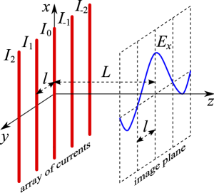
Figure 1: (color online) An array of line currents at §z=0§ with the image plane at $z=L$. We demand the electric field $E_{x}$ vanishing at discrete points $z=L$, $y=ml$, $m\neq 0$.

Physically, Eqs. (2) mean that we would like to concentrate the field at the image plane around point $y=0$ and at the same time have it completely vanishing at discrete points $y=ml$, $m\neq 0$. Next, we will look for such a distribution of currents that satisfies (2).

Considering a Fourier series with the discrete currents $I_{n}$ as its coefficients one can write

$$I_{n}={1\over 2\pi}\int\limits_{-\pi}^{\pi}{\cal J}(q)e^{-jnq}dq,$$ (3)

where ${\cal J}(q)$ is yet unknown function. Substituting (3) into (1) we obtain

$$E_{x}(ml,L)=-{k\eta\over 8\pi}\sum\limits_{n=-\infty}^{+\infty}H_{0}^{(2)}(k\sqrt{(n-m)^{2}l^{2}+L^{2}})\int\limits_{-\pi}^{\pi}{\cal J}(q)e^{-jnq}dq\\ =-{k\eta\over 8\pi}\int\limits_{-\pi}^{\pi}{\cal J}(q)e^{-jmq}\sum\limits_{n=-\infty}^{+\infty}H_{0}^{(2)}(k\sqrt{n^{2}l^{2}+L^{2}})e^{-jnq}\,dq.$$ (4)

Next, using the Poisson summation formula

$$\sum\limits_{n=-\infty}^{+\infty}H_{0}^{(2)}(k\sqrt{n^{2}l^{2}+L^{2}})e^{-jnq}\,dq=2j\sum\limits_{m=-\infty}^{+\infty}{e^{-{L\over l}\sqrt{(2\pi m-q)^{2}-k^{2}l^{2}}}\over\sqrt{(2\pi m-q)^{2}-k^{2}l^{2}}}\equiv{\cal K}(q),$$ (5)

where ${\cal K}(q)$ is a quickly converging series; the branch of the square root in (5) is such that $\sqrt{-1}=+j$. It is seen that ${\cal K}(-q)={\cal K}(q)$ and ${\cal K}(q+2\pi n)={\cal K}(q)$.

From (4) and (5) we get

$$E_{x}(ml,L)=-{k\eta\over 8\pi}\int\limits_{-\pi}^{\pi}{\cal J}(q){\cal K}(q)e^{-jmq}\,dq.$$ (6)

From (6) and the condition (2) it immediately follows that

$${\cal J}(q)=-{4E_{0}\over k\eta}{\cal K}(q)^{-1}.$$ (7)

Finally, sustituting (7) into (3) we get the complex amplitudes of the currents:

$$I_{n}=-{4E_{0}\over k\eta}\Psi(n),\quad\Psi(n)={1\over\pi}\int\limits_{0}^{\pi}{\cos nq\over{\cal K}(q)}\,dq,$$ (8)

where we have introduced the function $\Psi(n)$ that we will call elementary wavelet. In terms of it, condition (2) can be rewritten as

$$\sum\limits_{n=-\infty}^{+\infty}\Psi(n)H_{0}^{(2)}(k\sqrt{(n-m)^{2}l^{2}+L^{2}})=\left\{\begin{array}[]{lcl}1,\quad m&=&0,\\ 0,\quad m&\neq&0.\end{array}\right.$$ (9)

Now we can formulate a couple of lemmas.

Lemma 1

For any given electric field distribution $E_{x}(y_{n})$ defined at discrete points $y_{n}=nl$ in the image plane there exists a distribution of line currents defined at the points $y_{n}=nl$ in the source plane that produces exactly the given electric field distribution. This distribution of currents is

$$I_{n}=-{4\over k\eta}\sum\limits_{m=-\infty}^{\infty}E_{x}(ml)\Psi(n-m).$$ (10)

This lemma is obvious: it directly follows from the superposition principle and the solution of the problem considered above.

Lemma 2

$\Psi(n-m)$ form a complete system of linearly independent functions on an infinite set of discrete points so that any given distribution of line currents $I_{n}$ can be uniquely expanded into wavelet series

$$I_{n}=\sum\limits_{m=-\infty}^{\infty}C_{m}\Psi(n-m).$$ (11)

The proof of this lemma is given in Appendix.

Now from the above lemmas we can conclude that the distribution of the field produced by a planar periodic array of discrete sources is completely determined by the values of the same field taken at corresponding discrete points in any plane parallel to the array plane. Indeed, knowing the discrete values of the field one can reconstruct the currents in the source plane with the help of Lemma 10 and then calculate the field at any point of space using (1). Lemma 11 makes sure that the source distribution found in this way is unique.

Having said that we arrive at the following theorem which is in a sense analogous to the Kotelnikov sampling theorem.

Theorem 1

The electric field of the considered planar periodic array of line currents is completely determined by the values of the same field taken at certain discrete points in any plane parallel to the array plane and can be represented by the following formula:

$$E_{x}(y,z)=\sum\limits_{m=-\infty}^{+\infty}E_{x}(ml,L)\sum\limits_{n=-\infty}^{+\infty}\Psi(n-m)H_{0}^{(2)}(k\sqrt{(nl-y)^{2}+z^{2}}).$$ (12)

As said above, this formula is the result of substitution of Eq. (10) into Eq. (1).

From this theorem we see that it is impossible to produce arbitrary near-field distributions with an array of currents of a given period. The set of realizable distributions is determined by (12) and is, basically, a set of linear combinations of the fields created by the wavelets of currents (11). Thus, the structure period sets a limit on the amount of details that one can expect to observe in a near-field image. Although this fact is rather physically intuitive and has been mentioned in the literature before, the above theorem makes it explicit in mathematical terms.

Let us now discuss some properties of the introduced wavelet functions. The elementary wavelet is given by (8). When the period of the array is small compared to the wavelength and the parameter $L/l$ is large enough, the series ${\cal K}(q)$ converges very rapidly, so that only a few first terms of the series should be taken into account. For instance, for $kl\leq\pi/2$ and $L/l\geq 3$ it is enough to take only 3 terms of the series.

Example plots of the normalized elementary wavelets for two cases with different values of the parameters are given in Fig. 2(a, b). One can see that the normalized $\Psi(n)$ is practically purely imaginary, as the real part of it approaches zero for $kl\leq\pi/2$ and $L/l\geq 3$. On the plot there are also shown the distribution of current magnitudes of the source introduced by Merlin Merlin (2007): $|I_{n}|\propto 1/(1+n^{2}l^{2}/L^{2})$ and the distribution that we can obtain from our formulas when only a single term of the series (5) with $m=0$ is taken into account. We conclude that when $L/l\gg 1$ the source proposed by Merlin can be seen as a one-term approximation of our formulas. This approximation is valid only for small $n$ because $\Psi(n)$ decays quicker (exponentially) when $n\rightarrow\infty$.

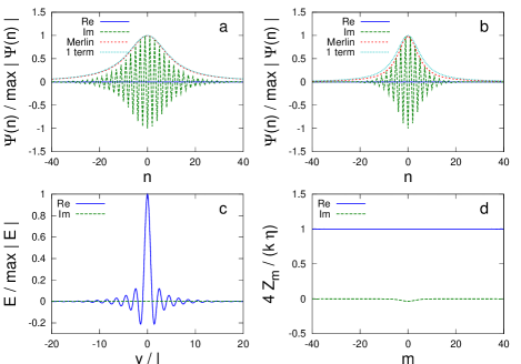
Figure 2: (color online) (a, b) The normalized elementary wavelets $\Psi(n)$ as functions of $n$. The parameters are: a) $L/l=10$, $kl=0.1\pi$; b) $L/l=5$, $kl=0.45\pi$. (c) The normalized electric field $E_{x}$ in the image plane as a function of $y/l$. The parameters are as in Fig. 2(b). (d) The second term of the total wire impedance $Z_{m}^{\rm tot}$ normalized to $k\eta/4$ as a function of $m$.

The field distribution in the image plane is depicted in Fig. 2(c). This function reminds of $\mbox{sinc}(y/l)$, however for large arguments it decays quicker (exponentially). One can see that the width of the near-field peak at zero level is $2l$, as expected.

Next we would like to consider how the introduced wavelets (which are certain distributions of line currents) can be physically realized. It is natural to represent a two-dimensional array of line currents with a grid of thin wires illuminated by an incident plane wave. As we would like to excite currents with alternating phases on the neighboring wires (see Fig. 2(a,b)) it is natural to load the wires with alternating reactive loads, so that the effective wire impedances and wire currents will change from wire to wire in the necessary way. Contrary to the scheme proposed in Grbic et al. (2008) we would like to separate the creation of the phase profile of the currents from the amplitude profile. Indeed, the characteristic scale of the amplitude profile $L$ can be much larger than the phase change scale $l$. In the example given in Fig. 2(a) these scales differ by 10 times, so that the phase scale can be subwavelength while the amplitude scale is not. Therefore, it is more practical to realize the amplitude profile with the conventional optical means by shaping the incident beam with diaphragms and/or lenses, while the phase profile can be realized with wire loading.

As a proof of concept let us calculate the interaction field and the local field in a wire array with currents distributed proportionally to $\Psi(n)$: $I_{n}=I_{0}[\Psi(n)/\Psi(0)]$ for the case depicted in Fig. 2(b). The interaction field at the $m$-th wire is

$$E_{x}^{\rm int}(ml,0)=-{k\eta I_{0}\over 4\Psi(0)}\sum\limits_{n=-\infty\atop n\neq m}^{+\infty}\Psi(n)H_{0}^{(2)}(|n-m|kl).$$ (13)

Given the incident field $E^{\rm inc}_{x}(y,z)$ the local field acting on the $m$-th wire can be expressed as $E^{\rm loc}_{m}=E^{\rm inc}_{x}(ml,0)+E_{x}^{\rm int}(ml,0).$ As we discussed above, we realize the necessary amplitude profile of the currents by shaping the incident field accordingly, so that $E^{\rm inc}_{x}(ml,0)=E^{\rm inc}_{0}{|\Psi(m)|/\Psi(0)}.$ Therefore, the total effective impedance (including the self-impedance and loading) per unit length of the $m$-th wire has to be

$$Z^{\rm tot}_{m}={E^{\rm loc}_{m}\over I_{m}}={E^{\rm inc}_{0}\over I_{0}}{|\Psi(m)|\over\Psi(m)}\\ -{k\eta\over 4\Psi(m)}\sum\limits_{n=-\infty\atop n\neq m}^{+\infty}\Psi(n)H_{0}^{(2)}(|n-m|kl).$$ (14)

The phase of the first term in (14) is alternating from wire to wire while its magnitude remains constant. Moreover, if $I_{0}$ is chosen to be in phase with $E^{\rm inc}_{0}$ then this impedance term is practically purely reactive (imaginary). The dependence of the second term on wire index is plotted in Fig. 2(d). One can see that the real part of this term is constant and equals the radiation resistance of a single wire. Indeed, for the self-impedance of a thin wire of radius $r$ we have Tretyakov (2003) $4Z_{\rm self}/(k\eta)=H_{0}^{(2)}(kr)\approx 1+j(2/\pi)\log[2/(\gamma kr)]$, where $\log(\gamma)\approx 0.5772$.

Another important property of it seen from Fig. 2(b) is that the imaginary part is also practically constant with $m$ . Moreover, for the chosen parameters it happens to be very close to zero. This means that in a real array of wires we can neglect the small difference in this part of the impedance and load all wires by loads of only two kinds, to account for alternating reactance of the constant magnitude in the first term of $Z_{m}^{\rm tot}$. When compared to Grbic et al. (2008) this greatly simplifies the structure. Moreover, our loaded wire grid is periodic with the period $2l$, therefore if the beam illuminating the array moves along $y$-axis by an integral number of periods, the subwavelength spot produced by the array will also move by the same number of periods. This important property is missing in the realizations proposed in Grbic et al. (2008); Eleftheriades and Wong (2008); Markley et al. (2008); Markley and Eleftheriades (2009).

To conclude, in this letter we have formulated a theorem on subwavelength imaging which is in a sense analogous to the Kotelnikov sampling theorem. In the process of derivation of this theorem we solved a problem about a distribution of currents in a two-dimensional array that produces a given subwavelegth near-field spot. The found distribution of line currents represents an elementary source wavelet. It has been shown that the source proposed in Merlin (2007); Grbic et al. (2008) can be understood as a one-term approximation of the elementary wavelet derived in this letter. We have also shown that if the necessary amplitude profile of the currents is realized by shaping the incident field by conventional optical means the remaining phase profile can be produced with a grid of thin wires loaded by reactive loads of only two kinds. When compared to structures considered by other authors such a periodically loaded wire grid appears to be much simpler to realize.

Appendix

We start with the proof of linear independence. Let us assume that there exists a non-trivial linear combination of wavelets such that

$$\sum_{m=-\infty}^{\infty}\alpha_{m}\Psi(n-m)=0,\quad\forall\,n\in{\cal Z}.$$ (15)

This linear combination defines a source distribution with all currents equal to zero: $I_{n}\equiv 0$, therefore, the field exited by these vanishing currents must also vanish everywhere.

From the other hand, (15) is a non-trivial linear combination, therefore there exists $\alpha_{p}\neq 0$. But then from the definition of $\Psi(n)$ it immediately follows that the electric field in the image plane at the point $y_{p}=pl$ is $E_{x}(y_{p})=-(k\eta/4)\alpha_{p}\neq 0$. We have arrived at a contradiction, therefore $\Psi(n-m)$ are linearly independent.

Completeness of the system of functions $\Psi(n-m)$ can be seen from the following. Consider the linear combination of wavelets (11) with coefficients given by $C_{m}=H_{0}^{(2)}(k\sqrt{(p-m)^{2}l^{2}+L^{2}})$. Then, denoting $s=n-m$ and using (9) we get for the currents

$$I_{n}=\sum_{s=-\infty}^{+\infty}H_{0}^{(2)}(k\sqrt{(s-(n-p))^{2}l^{2}+L^{2}})\Psi(s)=\left\{\begin{array}[]{lcl}1,\quad n&=&p,\\ 0,\quad n&\neq&p.\end{array}\right.$$ (16)

Since $p$ is arbitrary we see that the current localized at any point $y_{p}=pl$ can be expressed in terms of the wavelets, therefore any distribution of such currents can be expressed also.

References

- Pendry (2000) J. B. Pendry, Phys. Rev. Lett. 85, 3966 (2000).
- Grbic and Eleftheriades (2004) A. Grbic and G. V. Eleftheriades, Phys. Rev. Lett. 92, 117403 (2004).
- Alitalo et al. (2006a) P. Alitalo, S. I. Maslovski, and S. A. Tretyakov, J. Appl. Phys. 99, 064912 (2006a).
- Alitalo et al. (2006b) P. Alitalo, S. I. Maslovski, and S. A. Tretyakov, J. Appl. Phys. 99, 124910 (2006b).
- Maslovski et al. (2004) S. I. Maslovski, S. A. Tretyakov, and P. Alitalo, J. Appl. Phys. 96, 1293 (2004).
- Freire and Marqués (2005) M. J. Freire and R. Marqués, Appl. Phys. Lett. 86, 182505 (2005).
- Maslovski and Tretyakov (2003) S. I. Maslovski and S. A. Tretyakov, J. Appl. Phys. 94, 4241 (2003).
- Pendry (2008) J. B. Pendry, Science 322, 71 (2008).
- Merlin (2007) R. Merlin, Science 317, 927 (2007).
- Grbic et al. (2008) A. Grbic, L. Jiang, and R. Merlin, Science 320, 511 (2008).
- Eleftheriades and Wong (2008) G. V. Eleftheriades and A. M. H. Wong, IEEE Microw. Wireless Compon. Lett. 18, 236 (2008).
- Markley et al. (2008) L. Markley, A. M. H. Wong, Y. Wang, and G. V. Eleftheriades, Phys. Rev. Lett. 101, 113901 (2008).
- Markley and Eleftheriades (2009) L. Markley and G. V. Eleftheriades, IEEE Microw. Wireless Compon. Lett. 19, 137 (2009).
- Kotelnikov (1933) V. A. Kotelnikov, in Material for the First All-Union Conference on Questions of Communication (Izd. Red. Upr. Svyazi RKKA, Moscow, 1933).
- Shannon (1949) C. E. Shannon, Proc. Inst. Radio Eng. 37, 10 (1949).
- Tretyakov (2003) S. A. Tretyakov, Analytical Modelling in Applied Electromagnetics (Norwood, MA: Artech House, 2003).