About statistics of periods of continued fractions of quadratic irrationalities

Abstract

In this paper we answer certain questions posed by V.I. Arnold, namely, we study periods of continued fractions for solutions of quadratic equations in the form $x^{2}+px=q$ with integer $p$ and $q$, $p^{2}+q^{2}\leq R^{2}$. Our results concern the average sum of period elements and Gauss–Kuzmin statistics as $R\to\infty$.

Keywords  Continued fractions, quadratic irrationalities, Arnold conjecture, Gauss–Kuzmin statistics, Bykovskii’s theorem, “Nose-Hoover” algorithm, mediant.

Mathematical Subject Classification (2000) 11K50, 11J70.

1 Statement and discussion of obtained results

Any value $x\in{\mathbb{R}}$ is representable as a continued fraction (CF)

$$x=a_{0}+\cfrac{1}{a_{1}+\cfrac{1}{a_{2}+\ldots}}=[a_{0};a_{1},a_{2},\ldots],$$

where $a_{0}\in{\mathbb{Z}}$ (if $a_{0}=0$, then we omit it), $a_{i}\in{\mathbb{N}}$ for all $i\geq 1$. Let $i$ be a fixed position in the CF expansion and let $P_{i}(k)$ stand for the probability that $a_{i}=k$ with $x$ randomly chosen in the segment $[0,1)$. Hereinafter we understand the random choice as a realization of the uniform distribution. It is well known that according to the Gauss–Kuzmin theorem,

$$\lim_{i\to\infty}P_{i}(k)=\ln(1+\frac{1}{k(k+2)})/\ln 2.$$ (1)

The roots of the quadratic equation $x^{2}+px=q$, where $p,q\in{\mathbb{Z}}$, $\Delta=p^{2}+4q>0$, are expandable in a periodic CF. Let $x_{+}(p,q)=\sqrt{\Delta}/2-p/2$. The fractional part of this value $\{x_{+}(p,q)\}=x_{+}(p,q)-\lfloor x_{+}(p,q)\rfloor$ has no pre-period in the CF expansion: $\{x_{+}(p,q)\}=[[a_{1},\ldots,a_{T(p,q)}]]$. Here $T(p,q)$ is the length of the period of the CF for $x_{+}(p,q)$; denote the period itself $(a_{1},\ldots,a_{T(p,q)})$ by $a(p,q)$.

Let us adduce the Arnold conjecture about the Gauss–Kuzmin statistics for periods of CF of quadratic irrationalities ([1, problem 1993-11B], [2, 3, 4]):

Conjecture 1.  Choose an integer point $(p,q)$ in the circle of radius $R$ with the probability proportional to $T(p,q)$. Further, let us randomly choose $a_{i}$ from the corresponding set $a(p,q)$ (V.I. Arnold performs this two-step procedure immediately by the random choice from the union of sets $a(p,q)$). Then the probability that $a_{i}=k$ tends to $\ln(1+\frac{1}{k(k+2)})/\ln 2$ as $R\to\infty$.

Unfortunately, for some reasons, the proof of this conjecture performed by V.A. Bykovskii and his followers was not published. Below we describe the simple proof of the following theorem:

Theorem 1.  Let $w\in(0,1)$ be a fixed value. Let us randomly choose a fixed integer point $(p,q)$ in the circle of radius $R$. Further, let us choose from the corresponding set $a(p,q)$ the value $a_{i}$ with the probability proportional to $w^{i}$. Then the probability that $a_{i}=k$ tends to $(1-w)\sum_{i=1}^{\infty}P_{i}(k)w^{i-1}$ as $R\to\infty$. The limit of this sum with $w\to 1$ is the Gauss–Kuzmin statistics $\ln(1+\frac{1}{k(k+2)})/\ln 2$.

The latter part of this assertion, evidently, follows from the Kuzmin theorem (1) and the regularity of the Abel summation method [5]. We did not succeed to prove a variant of Theorem 1 with $w$ initially equal to 1.

Note that with the random choice of $(p,q)$ in the circle of radius $R$ the number $x_{+}(p,q)$ is not necessarily an irrational real value. In accordance with Theorem 1 the probability of this event tends to zero as $R\to\infty$. Let $\Omega_{R}$ stand for the set of pairs $(p,q)$ for which this event does not take place with fixed $R$.

In papers [3, 4] V.I. Arnold experimentally studied the value

$$\widehat{T}(R)=\sum_{(p,q)\in\Omega_{R}}T(p,q)/|\Omega_{R}|.$$

He established that

$$\widehat{T}(R)\sim\text{const}\ R\quad\text{ as $R\to\infty$.}$$ (2)

Let $T_{0}(q)=T(0,q)$ be the period of the CF for the square root of $q$. Put $\widehat{T}_{0}(Q)=\sum_{q=1}^{Q}T_{0}(q)/Q$. Some experts in the number theory studied the mean value of the mentioned kind experimentally; this enabled them to state the following conjecture: $\widehat{T}_{0}(Q)\sim\text{const}\sqrt{Q}\ln^{-\alpha}(Q)$, where $\alpha>0$ (see [6] and references therein).

Note that one can easily upper estimate $\widehat{T}_{0}(Q)$ [7]:

$$\widehat{T}_{0}(Q)<\text{const}\sqrt{Q}.$$

In [8] (see also [6]) E.P. Golubeva proves that the left-hand side of this inequality is asymptotically small in comparison with the right-hand one; moreover, if the extended Riemann conjecture is true, then the order of their difference is not less than $\ln(Q)^{\ln 2-\varepsilon}$. The bound

$$\widehat{T}_{0}(Q)>\text{\rm const}\ \sqrt{Q}\ln^{-\alpha}(Q)$$ (3)

would allow us to answer the famous Gauss question [9] about the growth of the number of classes of real quadratic fields. The known lower bound for $\widehat{T}_{0}(Q)$ is far from the right-hand side of (3). In [6] E.P. Golubeva proves only that $\widehat{T}_{0}(Q)>\text{const}\ln(Q)$.

Problem 5 listed in [10] implies the estimation of the growth rate of elements of the period of a CF. Let us adduce its exact statement [10, page 7].

Let $\widehat{a}(p,q)=\sum_{a_{i}\in a(p,q)}a_{i}/T(p,q)$, $A(R)=\sum_{(p,q)\in\Omega_{R}}\widehat{a}(p,q)/|\Omega_{R}|$. “The problem is to evaluate the growth rate of $A(R)$: is $A$ greater than $CR^{\alpha}$ for some positive $C$, $\alpha$ ? Or is it smaller than some $C(\ln R)^{\alpha}$ ?”.

Let us prove the following assertion.

Theorem 2.  Let us choose $a_{i}$ in the same way as in the statement of Conjecture 1; let $A^{\prime}_{R}$ stand for the mean value of the chosen number, that is,

$$A^{\prime}_{R}=\frac{\sum_{(p,q)\in\Omega_{R}}\sum_{a_{i}\in a(p,q)}a_{i}}{\sum_{(p,q)\in\Omega_{R}}T(p,q)}.$$ (4)

If correlation (2) or at least that $\widehat{T}(R)>\text{\rm const}\ R\,(\ln R)^{-\beta}$ analogous to inequality (3) takes place, then we have

$$A^{\prime}_{R}<C(\ln R)^{\alpha}.$$

The main idea of the proof of Theorem 1 is the representation of the probability under consideration as the Riemann integral. By applying the Weyl theorem to the uniformly distributed sequence $x_{+}(p,q)$ in Section 2 we easily prove the desired assertion.

The idea of the application of the Riemann integral sums was used implicitly for the proof of a similar correlation in the case of rational values with fixed denominator [12, Theorem 4.5.3.E]. However, in this case one usually applies another technique. An analog of Conjecture 1 for rational values $p/q$ was proved by M.O. Avdeeva and V.A. Bykovskii in [13]. The asymptotic validity of the Gauss–Kuzmin statistics in the case of a fixed denominator follows from results obtained by H. Heilbronn and J.W. Porter (see [14]). In  [15] A.V. Ustinov establishes the limit statistics for finite fractions whose divisors and denominators belong to an arbitrary expanding domain.

The proof of Theorem 2 is based on the upper estimate for $\sum_{a_{i}\in a(p,q)}a_{i}$ as a certain simple function of the discriminant $\Delta$. We prove this inequality (possibly, known by experts) with the help of a simple geometric construction that represents a symbiosis of the “Nose-Hoover” algorithm [2] and an explicit technique for defining values of an integer-valued sign-indefinite quadratic form [16].

Note that sign-indefinite quadratic forms correspond to hyperbolic operators. Symmetric properties of hyperbolic operators were studied in geometric terms by F. Aicardi ([17], see also [18, 19]). The algebraic approach to this topic is described in well-known papers [20, 21].

This paper is written under the bright impression of lectures delivered by V.I. Arnold [22, 23, 24] and a result of the performed numerical experiments.

2 Proof of Theorem 1.

Let $b$ be an arbitrary number from the segment $[0,1]$. Recall ([25]) that a sequence is said to be uniformly distributed, if among its first $N$ elements the quotient of terms whose fractional part is less than $b$ tends to $b$ as $N\to\infty$.

Lemma 1.  Let us enumerate numbers $x_{+}(p,q)$, $(p,q)\in\mathbb{Z}^{2}$, $p^{2}+4q>0$ in ascending order of the distance from the point $(p,q)$ to the origin of coordinates (in the case of equal distances the numeration is arbitrary). The obtained sequence is uniformly distributed.

Since $x_{+}(p,q)-x_{+}(-p,q)\in\mathbb{Z}$, in order to prove the lemma, suffice it to consider the terms of the sequence that correspond to points in the right half-plane. Lemma 1 easily follows from Lemma 2.

Lemma 2.  Let $n$ is a fixed integer number. The subsequence of the sequence from Lemma 1 that corresponds to points $(p,q)$ such that $n\leq q/p<n+1$, $p>0$ is uniformly distributed.

Proof of Lemma 2  Conditions $n\leq q/p<n+b$, $p>0$, $b\in[0,1]$ define the sector $S_{n,n+b}$ in the plane $(p,q)$. Instead of it, let us consider another domain $S^{\prime}_{n,n+b}$. The domain $S^{\prime}_{n,n+b}$ is defined by inequalities $np+n^{2}\leq q<(n+b)p+(n+b)^{2}$, with $p>-2n$ and inequalities $-p^{2}/4\leq q<(n+b)p+(n+b)^{2}$ with $-2n-b<p\leq-2n$ (see Fig. 1). One can easily make sure that the rays that define the boundaries of the domain $S^{\prime}$ are equiscalar lines of the function $x_{+}(p,q)$. Evidently, the condition $\{x_{+}(p,q)\}<b$ for points from $S^{\prime}_{n,n+1}$ is equivalent to their belonging to the subsector $S^{\prime}_{n,n+b}$.

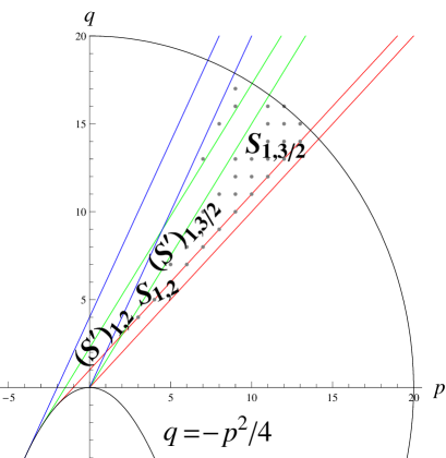
Figure 1: Domains considered in the proof of Lemma 2. The rays that bound the domain $S^{\prime}$ are tangent lines to the parabolic curve $q=-p^{2}/4$. Indicated are sets of points $M_{20,1,1/2}\cap M^{\prime}_{20,1,1/2}$ and $\bar{M}_{20,1,1/2}\cap\bar{M}^{\prime}_{20,1,1/2}$.

Let $M_{R,n,b}$ ($M^{\prime}_{R,n,b}$) stand for the set of integer points located inside the sector $S_{n,n+b}$ (the domain $S^{\prime}_{n,n+b}$) and the circle of radius $R$ centered at the origin of coordinates. Let $\bar{M}_{R,n,b}=M_{R,n,1}\setminus M_{R,n,b}$, $\bar{M}^{\prime}_{R,n,b}=M^{\prime}_{R,n,1}\setminus M^{\prime}_{R,n,b}$.

Evidently, for $R\to\infty$ we have $|M^{\prime}_{R,n,b}\cap M_{R,n,b}|/|M_{R,n,1}|\to b$, $|\bar{M}^{\prime}_{R,n,b}\cap\bar{M}_{R,n,b}|/|M_{R,n,1}|\to 1-b$, whence we obtain the assertion of Lemma 2.   $\Box$

The assertion of Lemma 1 follows from the inequality $|\bigcup_{n:|n|\leq N}M_{R,n,1}|/|M_{R,+}|>1-1/N$, where $M_{R,+}$ is the collection of all integer points located in the half-circle of radius $R$.

Let us now immediately prove Theorem 1. Let $i,k\in\mathbb{N}$, let $I^{i}_{k}(x)$ stand for the indicator function of the set of points $x$ from the segment $[0,1]$ for which the $i$-th position in the CF is occupied by the number $k$. This set and its complement are representable as unions of countable numbers of intervals [26]. Consequently, the function $I^{i}_{k}(x)$ is countably continuous and therefore it is Riemann integrable. The function $f_{k,w}(x)=(1-w)\sum_{i=1}^{\infty}I^{i}_{k}(x)w^{i-1}$ has the same property. The integral of this function

$$\int_{0}^{1}f_{k,w}(x)\,dx=(1-w)\sum_{i=1}^{\infty}P_{i}(k)w^{i-1}$$ (5)

equals the probability of the event $A$: $a_{j}=k$ with the random choice of the number $x$ in the segment $[0,1)$. Here $j$ is chosen randomly, namely, $\text{Prob}(j=i)=(1-w)w^{i-1}$, $i=1,2,3,\ldots$.

We can calculate the Riemann integral (5) with the help of the Weyl theorem [25]. In accordance with this theorem the frequency of the event $A$ for the first $N$ terms of a uniformly distributed sequence tends to its probability. Taking into account the fact that the CF for $\{x_{+}(p,q)\}$ has no pre-period, we obtain the assertion of Theorem 1.  $\Box$

3 Proof of Theorem 2

We remind [2] that the “Nose-Hoover” algorithm for finding a CF of a real number $x$, $x>0$, is reduced to the geometric method which constructs the boundary of the convex shell of the set of integer nonnegative points $(u,v)$ located above (below) the straight line $v=xu$. Let $\boldsymbol{e}_{0}$ stand for the vector $(0,1)$, $\boldsymbol{e}_{1}=(1,0)$. Put

$$\boldsymbol{e}_{n+1}=\boldsymbol{e}_{n-1}+a_{n-1}\boldsymbol{e}_{n},\quad n=1,2,\ldots,$$ (6)

where $a_{n-1}$ is the maximal integer such that the vector $\boldsymbol{e}_{n+1}$ lies below (for odd $n$) or above (for even $n$) the straight line $v=xu$. Klein noted that $a_{n}$, $n=0,1,\ldots$, coincide with partial quotients of the CF of the number $x$. The geometric algorithm results in two polylines which represent parts of sails of the CF.

Let $x>1$. We need a slightly modified algorithm which results in one infinite polyline $L$, originating at the point $(1,1)$, whose segments are the vectors $a_{n-1}\boldsymbol{e}_{n}$, $n=1,2,\ldots$. Evidently, $\boldsymbol{e}_{n+1}+\boldsymbol{e}_{n}=\boldsymbol{e}_{n}+\boldsymbol{e}_{n+1}$. Consequently, if in the standard “Nose-Hoover” algorithm  (6) we add the extra vector $\boldsymbol{e}_{n}$ and thus go out of the line $v=xu$ (i. e., we consider the vector $\boldsymbol{e}_{n-1}+(a_{n-1}+1)\boldsymbol{e}_{n}$), then we get the first integer point on the segment of the polyline of another sail constructed at step $n+1$. This fact justifies a simple geometric algorithm which constructs the polyline $L$.

We begin the construction process with the point $(1,1)$; it is convenient to connect it with the origin of coordinates by the segment which does not enter in $L$. As the “constructive” term at the first ($n$th) step we choose the vector $\boldsymbol{e}_{1}$ (the vector $\boldsymbol{e}_{n}$). We add this vector till we go out of the line $v=xu$. The newly added vector $\boldsymbol{e}_{n+1}$ is directed from the origin of coordinates to the point obtained as a result of the latter addition up to the step out of the line. See Fig. 2 for the first segments of the polyline for $x=\sqrt{2}$. The zero partial quotient (i. e., $\lfloor x\rfloor$) differs from zero. In order to provide the correspondence to the indices of partial quotients, it is also convenient to begin the numeration of segments of the polyline $L$ with zero.

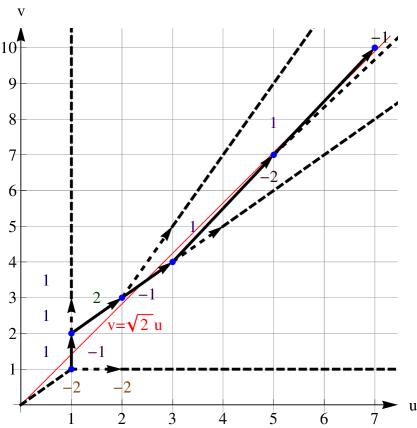
Figure 2: The gradual “Nose-Hoover” algorithm for $x=\sqrt{2}$

Let us consider the approximation of a number $x$ by mediants. Let $f_{1}=\frac{v_{1}}{u_{1}}$, $f_{2}=\frac{v_{2}}{u_{2}}$ be irreducible fractions such that $v_{1},u_{1},v_{2},u_{2}\geq 0$ and $f_{1}<f_{2}$. Let us define the operation $\downarrow$ of finding the mediant (the “insertion” operation) by the formula $f_{1}\downarrow f_{2}=\frac{v}{u}$, where $v=v_{1}+v_{2}$, $u=u_{1}+u_{2}$. Earlier we used the denotation introduced by A.A. Kirillov. Evidently, in the geometric representation of the fraction $\frac{v}{u}$ as the integer vector $(u,v)$ the operation $\downarrow$ corresponds to the addition of vectors $(u_{1},v_{1})$ and $(u_{2},v_{2})$. The obtained diagonal of the parallelogram appears to be “inserted” between its sides.

Let $x\in(f_{1},f_{2})$, $f_{3}=f_{1}\downarrow f_{2}$. Since $f_{3}\in(f_{1},f_{2})$, one can treat $f_{3}$ as an approximation of the number $x$. If $x\in(f_{1},f_{3})$, then we put $f_{4}=f_{1}\downarrow f_{3}$, otherwise we do $f_{4}=f_{3}\downarrow f_{2}$. The process of the approximation of the number $x$ by mediants consists in the repetition of these operations for the corresponding intervals.

The condition $x>0$ means that $x\in\left(\frac{0}{1},\frac{1}{0}\right)$. The initial approximation of $x$ for such an interval is the fraction $\frac{1}{1}$. One can easily see that for the mapping

the fraction $$\frac{v}{u}\quad\leftrightarrow\quad (u,v)$$ the point

the geometric representation of the algorithm for approximating the number $x$ by mediants is completely identical to the algorithm for constructing the polyline $L$. The technical distinction consists in the following fact: earlier we constructed each segment of the polyline $L$ “at once”, but now it “grows gradually” due to the stepwise addition of the next vector $\boldsymbol{e}_{i}$.

Further we consider a simplified version of this algorithm for the quadratic irrationality $x_{+}(p,q)$. We will need it for the proof of the next assertion.

Lemma 3.  For $n\in\mathbb{N}$ put $D(n)=\sum_{u=1}^{\lfloor\sqrt{n}\rfloor}\tau(n-u^{2})$, where $\lfloor\cdot\rfloor$ is the integer part, $\tau(m)$ is the quantity of divisors of the number $m$. We have the inequality

$$\sum_{a_{i}\in a(p,q)}a_{i}\leq f(\Delta/4),\qquad\text{ where\quad$\Delta=p^{2}+4q$,\phantom{nbbnbnbnb}}$$ (7)

$$f(n)=2D(n)+\tau(n),\text{if $n$ is integer;}$$ (8)

$$f(n)=2\mathop{\sum\limits_{i\in\{1,3,\ldots\}}}\limits_{i^{2}<4n}\tau(n-i^{2}/4),\text{ otherwise. }$$ (9)

In the case of an odd period $T(p,q)$ one can improve this bound, namely, divide the right-hand side of inequality (7) by two.

Proof of Lemma 3  Note that $\{x_{+}(p,q)\}=\{x_{+}(p+2,q-p-1)\}$, therefore, without loss of generality, we assume that $p=0$ or $p=1$, here $x_{+}(p,q)>1$ (the special case $x_{+}(1,1)$ is evident) and the second root of the quadratic equation is negative.

Let us apply to $x_{+}(p,q)$ the gradual “Nose-Hoover” algorithm described above. Let $(u_{n},v_{n})$ stand for the $n$th integer point on the polyline $L$, $n=0,1,2,\ldots$. We obtain it at the $n$th step of the gradual “Nose-Hoover” algorithm. In Fig. 2, for example, $(u_{0},v_{0})=(1,1)$, $(u_{1},v_{1})=(1,2)$, $(u_{2},v_{2})=(2,3)$, $(u_{3},v_{3})=(3,4)$, $(u_{4},v_{4})=(5,7)$, etc.

Let us draw one more vector which originates from the point $(u_{n},v_{n})$; denote it by $\boldsymbol{e}^{\prime}_{n}$. The vector $\boldsymbol{e}^{\prime}_{n}$ is defined by the condition $\boldsymbol{e}^{\prime}_{n}+\boldsymbol{e}_{i}+\boldsymbol{e}^{\prime\prime}_{n}=0$, where $\boldsymbol{e}_{i}$ is the vector which originates from the point $(u_{n},v_{n})$ and goes along the polyline $L$, $\boldsymbol{e}^{\prime\prime}_{n}=-(u_{n},v_{n})$ (we considered this vector earlier). The collection of vectors $\{\boldsymbol{e}^{\prime}_{n},\boldsymbol{e}_{i},\boldsymbol{e}^{\prime\prime}_{n}\}$, where each one is defined accurate to the multiplier $(-1)$, is a superbasis [16]. This means that any pair of these vectors generates the whole integer lattice. The transition from the point $(u_{n},v_{n})$ to that $(u_{n+1},v_{n+1})$ corresponds to the replacement of one superbasis with another one; the latter differs from the initial superbasis only in one of three its elements. Thus, for the polyline $L$ in Fig. 2 the initial superbasis is $\{(0,1),(1,0),(1,1)\}$, the 1st one is $\{(1,1),(1,0),(1,2)\}$, the 2nd one is $\{(1,2),(1,1),(2,3)\}$, the 3rd one is $\{(1,1),(2,3),(3,4)\}$, etc.

Let us extend vectors $\boldsymbol{e}^{\prime}_{n}$ up to the rays which originate at the points $(u_{n},v_{n})$. As a result, the first quadrant appears to be divided onto disjoint connected domains (see Fig. 2). Let us associate each vector $(u_{n},v_{n})$ with a domain, whose boundary contains all points of polylines which include the vector $(u_{n},v_{n})$ in the corresponding superbasis. In the picture these domains look like narrow “crevices” located at the north-east of the points $(u_{n},v_{n})$. We associate the domains which border on the coordinate axes with the unit vectors of these axes.

We have

$$\text{$(u_{n},v_{n})$ is located above the line $v=x_{+}(p,q)u$}\ \Longleftrightarrow\ v_{n}^{2}+pv_{n}u_{n}>qu_{n}^{2}.$$ (10)

Let us write the values of the quadratic form $v^{2}+pvu-qu^{2}$ at the points $(u_{n},v_{n})$ in the corresponding domain. See Fig. 2 for the result obtained in the case $p=0$, $q=2$ (the upper right corner of the figure contains the value calculated at the point $(5,7)$). From (10) it follows that the points of the polyline $L$ belong to boundaries of domains with positive and negative values. The collection of superbases which correspond to these points is called the river of the quadratic form [16].

Let us adduce the main result of the theory of quadratic forms which enables one to make the calculation of the period of a CF much easier. Using the values of the quadratic form at three vectors from any superbasis, one can easily restore the CF. To put it more precisely, the following correlation [16] is true. Let domains associated with values $a,b,c,d$ of the quadratic form be located in accordance with Fig. 3.

Figure 3: The arithmetic progression rule

Then values $d,a+b,c$ form an arithmetic progression. Moreover, if $h$ is the common difference of this progression, then

$$h^{2}/4-ab=\Delta/4.$$ (11)

Therefore, using the values $(a,b)$ for two neighboring domains with different signs separated by the polyline $L$, and the value $h$, one can unambiguously restore all subsequent and previous values of partial quotients of the CF, moving along the river of the quadratic form (see the figures in Chapter 1 of book [16]).

step number	0	1	2	3	4
$a$ is the value located at the north west of $L$	1	2	1	1	1
$b$ is the value located at the south east of $L$	-1	-1	-1	-2	-1
$h$ is the common difference of the arithmetic progression	2	0	-2	0	2
the number of a segment of the polyline	0	1	1	2	2

Table 1: All values of $(a,b,h)$ for the polyline represented in Fig. 2

Let us now immediately prove the inequalities (7). They follow from correlation (11). Assume that at step $n_{1}$ we get the same parameters of the arithmetic progression as those obtained at step $0$. Such a step exists because the algorithm is invertible. Let $l_{1}$ stand for the number of the polyline segment which contains the point $(u_{n_{1}},v_{n_{1}})$. Then a part of the CF $a_{1},a_{2},\ldots,a_{l_{1}}$ becomes periodic. In addition, the number $l_{1}$ is even, because the points $(u_{0},v_{0})$ and $(u_{n_{1}},v_{n_{1}})$ are located to one side of the polyline $L$. In the case of an odd period the sequence $a_{1},a_{2},\ldots,a_{l_{1}}$ contains at least two repeating subsequences. In accordance with the algorithm we have $\sum_{i=1}^{l_{1}}a_{i}=n_{1}$. Therefore, suffice it to estimate the number of all possible triplets $(a,b,h)$ which satisfy (11). The obtained bound obeys formulas (8,9). The multiplier 2 in the right-hand sides of these formulas appears, because we have to take into account various signs of $h$, and the term $\tau(\Delta/4)$ does when we consider the case $h=0$. Lemma 3 is proved.   $\Box$

Remark   In the proof of Lemma 3 we established that CF for $\{x_{+}(p,q)\}$ has no pre-period.

Let us complete the proof of Theorem 2. Formally speaking, the Dirichlet theorem (the equality $\sum_{u=1}^{n}\tau(u)/n=\ln n+(2\gamma-1)+O(1/\sqrt{n})$) does not imply that $D(n)\sim\sqrt{n}\ln n$, because the values of the function $\tau$ are not uniform. A more accurate bound is

$$D(n)=O(\ln^{3}(n)\sqrt{n})$$

(see [7] and references therein). This, evidently, implies that $f(n)=O(\ln^{3}(n)\sqrt{n})$. Taking the sum over all possible values of $(p,q)$, we obtain that the numerator of fraction (4) equals $O(R^{3}\ln^{3}(R))$, whereas the denominator by assumption is greater than $\text{\rm const}\ R^{3}\,(\ln R)^{-\beta}$. Theorem 2 is proved.  $\Box$

References

- [1] Arnold VI (2004) Arnold’s Problems. Springer, Berlin; PHASIS, Moscow
- [2] Arnold VI (2000) Tsepnie drobi (Continued fractions). Moscow Center for Continuous Mathematical Education, Moscow
- [3] Arnold VI (2007) Continued fractions of square roots of rational numbers and their statistics. Russ Math Surv 62(5):843–855
- [4] Arnold VI (2008) Statistics of Periods of Continued Fractions of Quadratic Irrationalities. Izv. RAN. Ser. Matem., 72(1), pp 3–38
- [5] Hardy GH (1949) Divergent Series. Oxford University Press, Oxford
- [6] Golubeva EP (1987,1988) The lengths of periods of the expansion in a continuous fraction of quadratic irrationalities and the numbers of classes of real quadratic fields. I, II. Zap. nauch. semin. LOMI, 160, pp 72–81; 168, pp 11–22
- [7] Beceanu M (2003) Period of the Continued Fraction of . Junior Thesis, Princeton University, Princeton, http://www.math.princeton.edu/mathlab/jr02fall/Periodicity/mariusjp.pdf
- [8] Golubeva EP (1984) The length of the period of a quadratic irrationality. Matem. Sborn., 123:1, pp 120–129
- [9] Venkov BA (1970) Elementary Number Theory. Wolters-Noordhoff, Groningen
- [10] Arnold VI (2008) Problems for the Seminar, ICTP, 2007-2008. Trieste. http://www.pdmi.ras.ru/ arnsem/Arnold/prob08.pdf
- [11] Lerner EYu (2008) Statistics of incomplete quotients of continued fractions of quadratic irrationalities. Preprint. http://xxx.lanl.gov/abs/0810.0718
- [12] Knuth DE (1997) The Art of Computer Programming, V.2. Addison-Wesley Professional
- [13] Avdeeva MO and Bykovskii VA (2002) Solution of the Arnold Problem on Gauss–Kuzmin Statistics. Preprint, Dal’nauka, Vladivostok
- [14] Ustinov AV (2008) The number of solutions to the comparison located below the graph of a twice continuously differentiable function. Algebra i Analiz, 20: 5, pp 186–216
- [15] Ustinov AV (2005) Gauss–Kuz’min Statistics for Finite Continued Fractions. Fundam. and Appl. Math., 11:6, pp 195–208
- [16] Conway JH (1997) The Sensual (Quadratic) Form. Carus Mathematical Monographs 26, Mathematical Association of America, Washington
- [17] Aicardi F (to appear) The sails of the SL(2,Z) operators and their symmetries. Funct Anal Other Math
- [18] Aicardi F (2007) Symmetries of quadratic forms classes and of quadratic surds continued fractions. Part II: Classification of the periods’ palindromes. arXiv:0708.2082v3 [math.GM]
- [19] Karpenkov ON (2007) On determination of periods of geometric continued fractions for twodimensional algebraic hyperbolic operators. arXiv:0708.1604v1 [math.NT]
- [20] Lewis J, Zagier D (1997) Period functions and the Selberg zeta function for the modular group. In: The mathematical beauty of physics, Saclay, 1996. Adv Ser Math Phys, 24. World Sci, River Edge, pp 83–-97
- [21] Manin YuI, Marcolli M (2002) Continued fractions, modular symbols, and noncommutative geometry. Selecta Math (N S) 8(3):475–521
- [22] Arnold VI (2007) Quadratic Irrational Numbers, Their Continued Fractions and Palindromes. Lectures of the Summer School “Modern Mathematics”, Dubna. http://www.mathnet.ru
- [23] Arnold VI (2007) Statistics of Periodic and Multidimensional Continued Fractions. Report at the International Conference “Analysis and Singularities”, Moscow. http://www.mathnet.ru
- [24] Arnold VI (2008) Continued Fractions of Square Roots of Integer Numbers. Lectures of the Summer School “Modern Mathematics”, Dubna. http://www.mathnet.ru
- [25] Kuipers L and Niederreiter H (1974) Uniform distribution of sequences. Wiley, New York
- [26] Khinchin AYa (1997) Continued Fractions. Dover, New York