Limit conditional distributions for bivariate vectors
with polar representation

Abstract

We investigate conditions for the existence of the limiting conditional distribution of a bivariate random vector when one component becomes large. We revisit the existing literature on the topic, and present some new sufficient conditions. We concentrate on the case where the conditioning variable belongs to the maximum domain of attraction of the Gumbel law, and we study geometric conditions on the joint distribution of the vector. We show that these conditions are of a local nature and imply asymptotic independence when both variables belong to the domain of attraction of an extreme value distribution. The new model we introduce can also be useful to simulate bivariate random vectors with a given limiting conditional distribution.

Keywords: Conditional excess probability; conditional extreme-value model; $\Gamma$-varying tail; asymptotic independence; elliptic distributions; second order correction.

1 Introduction

In many practical situations, there is a need of modeling multivariate extreme events. Extreme means, roughly speaking, that no observations are available in the domain of interest, and that extrapolations are needed. Multivariate extreme value theory provides an efficient mathematical framework to deal with these problems in the situation where the largest values of the variables of interest tend to occur simultaneously. This situation is referred to as asymptotic dependence in extreme value theory. In this case, probabilities of simultaneous large values of the components of the vector can be approximated and estimated by means of the multivariate extreme value distributions. In the opposite case of asymptotic independence, the approximate probability for two or more components being simultaneously large given by the standard theory is zero. Refinements of the standard theory are thus needed.

One refinement is the concept of hidden regular variation introduced by Resnick (2002). Another approach is studying, if it exists, the limiting distribution of a random vector conditionally on one component being large. See Heffernan and Resnick (2007). Formally stated in the bivariate case, this corresponds to assuming that there exist functions $m$, $a$ and $\psi$, and a bivariate distribution function (cdf) $K$ on $[0,\infty)\times(-\infty,\infty)$ with non degenerate margins such that

$$\lim_{t\to\infty}\mathbb{P}(X\leq t+\psi(t)x\;;Y\leq m(t)+a(t)y\mid X>t)=K(x,y)\;,$$ (1)

at all points of continuity of $K$. Das and Resnick (2008) introduced the terminology of conditional extreme-value (CEV) model. Note that Condition (1) implies that $X$ belongs to a max-domain of attraction. More properties can be found in Section 3.1, where in particular the relationship between CEV models and usual multivariate extreme value (EV) models is explicited. Statistical applications of the conditional model on various domains are discussed in several papers: see Heffernan and Tawn (2004) for a study on air quality monitoring, Abdous et al. (2008) and Fougères and Soulier (2008) for an insight into financial contagion, and Das and Resnick (2009) for an application on Internet traffic modeling.

An important issue that must be addressed is to study models under which Condition (1) holds. The aim of this contribution is to review existing models and exhibit new ones satisfying (1). We restrict our attention to bivariate random vectors for simplicity of exposition. We focus on the case where the conditioning variable belongs to the domain of attraction of the Gumbel distribution. The reason for that is that, as mentioned later, this situation is, in the models we consider, strongly related to the asymptotic independence, which is precisely the case where there is an advantage to work with CEV models instead of EV models (cf. Section 3.1). Our work is an attempt to motivate the use of CEV models by exhibiting a class of bivariate models that satisfy Condition (1).

In Section 2, we review the existing literature. In Section 3 we study new models for bivariate vectors $(X,Y)$ with a polar representation $R(u(T),v(T))$ where $R$ is a nonnegative random variable in the domain of attraction of the Gumbel law, independent of the random variable $T$, and the functions $u$ and $v$ are a parametrization of a certain curve. This model includes many models already studied in the literature, and in particular the bivariate elliptical distributions. Our main result (Theorem 3 in Section 3) shows that the local geometric nature of this curve around the maximum of $u$ determines the existence and form of the limiting distribution in (1). Our result covers situations that are more general than the results of Balkema and Embrechts (2007). In particular, as a consequence of their local nature, our assumptions do not imply that the conditioned variable ($Y$) belongs to the domain of attraction of a univariate extreme value distribution. Thus these polar distributions may not be imbedded in a standard multivariate extreme value model. But when they are, we show that they are asymptotically independent. In order to prove this, we extend (Das and Resnick, 2008, Proposition 4.1). Finally, following Abdous et al. (2008) we also study a second order correction for the asymptotic approximation (1). Section 4 contains the proof of Theorem 3. Some additional auxiliary results are given and proved in Section 5.

2 Elliptical and asymptotically elliptical distributions

Early results providing families of distributions that satisfy (1) were obtained by Eddy and Gale (1981) for spherical distributions and by Berman (1983) for bivariate elliptical distributions. Multivariate elliptical distributions and related distributions were investigated by Hashorva (2006); Hashorva et al. (2007). One essential feature of elliptical distributions is that the level sets of their density are ellipses in the bivariate case, or ellipsoids in general. Such geometric considerations have been deeply investigated and generalized in many directions by Barbe (2003) and Balkema and Embrechts (2007). It must be noted that these geometric properties will be ruined by transformation of the marginal distributions to prescribed ones. Another specific feature of the elliptical and related models is that the property of asymptotic dependence or independence is related to the nature of the marginal distributions. If they are regularly varying, then the components are asymptotically dependent; if the marginal distributions belong to the maximum domain of attraction of the Gumbel distribution, then the components are asymptotically independent.

We start by recalling some definitions that will be used throughout the paper. A nondecreasing function $g$ is said to belong to the class $\Gamma$ or to be $\Gamma$-varying (Resnick, 1987, Definition 0.47), if there exists a positive function $\psi$ such that

$$\lim_{x\to x_{1}}\frac{g(x+\psi(x)t)}{g(x)}=\mathrm{e}^{t}\;.$$

It is well known (cf. De Haan and Ferreira (2006, Theorem 1.2.5)) that a random variable $X$, with cdf $F$ and upper limit of the support $x_{1}$, is in the max-domain of attraction of the Gumbel distribution if and only if $1/(1-F)$ is $\Gamma$-varying, i.e.

$$\lim_{x\to x_{1}}\frac{1-F(x+\psi(x)t)}{1-F(x)}=\mathrm{e}^{-t}\;.$$ (2)

The function $\psi$ is called an auxiliary function. It is defined up to asymptotic equivalence and necessarily satisfies $\psi(x)=o(x)$ if $x_{1}=\infty$ and $\psi(x)=o(x_{1}-x)$ if $x_{1}<\infty$. In the sequel, for notational simplicity, we only consider the case $x_{1}=\infty$. The modifications to be made in the case $x_{1}<\infty$ are straightforward, and the main change is that the rates of convergence must be expressed in terms of $\psi(x)$ instead of $\psi(x)/x$. The function $\psi$ is self-neglecting (or Beurling slowly varying, cf. Bingham et al. (1989, Section 2.11)), i.e. for all $t>0$,

$$\lim_{x\to\infty}\frac{\psi(x+\psi(x)t)}{\psi(x)}=1\;.$$

Two random variables $X$ and $Y$ such that $(X,Y)$ belongs to the maximum domain of attraction of a bivariate extreme value distribution $G$ are said to be asymptotically independent if $G$ has independent marginals. (See e.g. (De Haan and Ferreira, 2006, Section 6.2)).

In the following two subsections, we recall the results on elliptic distributions and we state a bivariate version of a general result of Balkema and Embrechts (2007) which provides geometric sufficient conditions for (1) to hold. We also point out and illustrate the local nature of the sufficient condition formulated by Balkema and Embrechts (2007), in the case of $\Gamma$-varying upper tails.

2.1 Elliptical distributions

Consider a bivariate elliptical random vector, i.e. a random vector $(X,Y)$ that can be expressed as

$$(X,Y)=R(\cos\Theta,\rho\cos\Theta+\sigma\sin\Theta)$$ (3)

with $\sigma^{2}=1-\rho^{2}$, in terms of a positive random variable $R$ called “radial component” and an “angular” random variable $\Theta$ uniformly distributed on $[0,2\pi)$. The following result was originally proved in the case $\rho=0$ as a technical lemma under restrictive conditions in Eddy and Gale (1981). The general result was first proved in Berman (1983) in the bivariate case (see also Berman (1992) and Abdous et al. (2005)) and Hashorva (2006) in a multivariate setting. Throughout the paper $\Phi$ will denote the cdf of the standard normal distribution.

Theorem 1 (Berman (1983)).

Let $(X,Y)$ be an elliptical random vector as defined in (3). If the radial component $R$ is in the domain of attraction of the Gumbel law, i.e. its survival function $1-H$ satisfies (2) with auxiliary function $\psi$, then $X$ and $Y$ are also in the domain of attraction of the Gumbel law and

$$\lim_{t\to\infty}\mathbb{P}(X\leq t+\psi(t)x\;,Y\leq\rho t+\sqrt{t\psi(t)}y\mid X>t)=(1-\mathrm{e}^{-x})\Phi(y)\;.$$ (4)

Comments on Theorem 1

The fact that $X$ has $\Gamma$-varying upper tails follows from (4) by taking $y=\infty$. Since the same result holds with reversed roles for $X$ and $Y$, the consistency result (Das and Resnick, 2008, Theorem 2.2) implies that $(X,Y)$ belongs to the domain of attraction of a bivariate extreme value distribution. Moreover, since the limiting distribution in (4) has two independent marginals, $X$ and $Y$ are asymptotically independent, i.e. the limiting extreme value distribution is the product of its marginal distributions. See also Hashorva (2005, Section 3.2) for a proof of this property in a related context. In the case where $R$ has a regularly varying tail, the limiting distribution is not a product and the vector $(X,Y)$ is asymptotically dependent. See e.g. (Abdous et al., 2005, Theorem 1, part (i)). As mentioned in the introduction, we do not develop this case.

If the radial component $R$ has a density $h$, then the vector $(X,Y)$ has the density $f$ defined by

$$f(x,y)=\frac{h(\sqrt{x^{2}+(y-\rho x)^{2}/\sigma^{2}})}{\sqrt{x^{2}+(y-\rho x)^{2}/\sigma^{2}}}\;.$$

The level lines of the density are homothetic ellipses $x^{2}+(y-\rho x)^{2}/\sigma^{2}=c^{2}$.

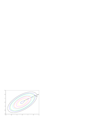
Figure 1: Level lines of the density of an elliptical distribution. The slope of the straight line is $\rho=.6$.

This result can be generalized in two directions: either by weakening the assumptions on the level lines of the density or by extending the representation (3). The first generalization will be considered in the following subsection, and the second one in Section 3.

2.2 Asymptotically elliptical distributions

In this section, we state a bivariate version of Balkema and Embrechts (2007, Theorem 11.2). We first need the following definition taken from Balkema and Embrechts (2007, Section 11.2).

Definition 1.

A function $L:\mathbb{R}^{2}\to\mathbb{R}_{+}$ belongs to the class $\mathcal{L}$ if for all $(x,y)\in\mathbb{R}^{2}$,

$$\lim_{||(\xi,\zeta)||\to\infty}\frac{L(x+\xi,y+\zeta)}{L(\xi,\zeta)}=1\;,$$

for any norm $||\cdot||$ on $\mathbb{R}^{2}$.

Assumption 1.

The random vector $(X,Y)$ has a density $f$ such that

$$f(x,y)=\mathrm{e}^{-I(x,y)}L(x,y)\;,$$ (5)

where $L\in\mathcal{L}$, and the function $I$ satisfies:

$$I(x,y)=p\circ n(x,y)\;,$$

$$p(r)=\int_{0}^{r}\frac{\mathrm{d}s}{\psi(s)}\;,$$ (6)

$\psi$ is absolutely continuous with $\lim_{x\to\infty}\psi^{\prime}(x)=0$ and $n:\mathbb{R}^{2}\to\mathbb{R}$ is 1-homogeneous, $n^{2}$ is twice differentiable and the Hessian matrix of $n$ is positive definite.

Theorem 2 (Balkema and Embrechts (2007)).

Under Assumption 1, $X$ and $Y$ are in the domain of attraction of the Gumbel law and satisfy (2) with auxiliary function $\psi$, are asymptotically independent, and there exist real numbers $\rho$ and $\sigma$ such that

$$\lim_{t\to\infty}\mathbb{P}(X\leq t+\psi(t)x\;;Y\leq\rho t+\sigma\sqrt{t\psi(t)}y\mid X>t)=(1-\mathrm{e}^{-x})\Phi(y)\;.$$ (7)

This result shows that Assumption 1 is a sufficient condition for the limit (1) to hold, with $m(x)=\rho x$, $a(x)=\sigma\sqrt{x\psi(x)}$ and $K(x,y)=(1-\mathrm{e}^{-x})\Phi(y)$. The constants $\rho$ and $\sigma$ are characterized by the second order expansion of the function $n$

$$n(1+x,\rho+\sigma y)=1+x+y^{2}/2+o(x^{2}+y^{2})\;.$$

This condition implies that the tangent at the point $(1,\rho)$ to the curve $n(\xi,\zeta)=1$ is vertical. Note that the level lines of the function $n$ are not those of the density $f$ defined in (5), unless the function $L$ is constant, but, loosely speaking, the level lines of $f$ converge to those of $n$. Theorem 2 implies Theorem 1 when the radial distribution is absolutely continuous.

Example 1.

Let $h$ and $g$ be density functions defined on $[0,\infty)$ and $[-\pi/2,\pi/2]$, respectively. The function $f$ defined by

$$f(x,y)=\frac{h(x^{2}+(y-\rho x)^{2}/(1-\rho^{2}))}{\sqrt{x^{2}+(y-\rho x)^{2}/(1-\rho^{2})}}\;g\circ\arctan((y-\rho x)/x\sqrt{1-\rho^{2}})$$ (8)

is then a bivariate density function on $\mathbb{R}^{2}$. If $g$ is a constant, then $f$ is the density of an elliptical vector. If $h$ can be expressed as in (6) and if $g$ is continuous and bounded above and away from zero, then $f$ satisfies Assumption 1. Figure 2 shows the level lines of such a density, with $\rho=.6$, $h(t)=\exp(t^{2}/2)/\sqrt{2\pi}$ and $g(t)=c\{1+[t^{2}-(\pi/4)^{2}]^{2}\}$. The level lines seem to be asymptotically homothetic.

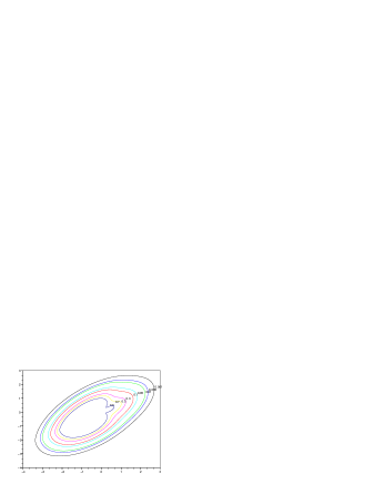
Figure 2: Level lines of the density given by (8).

It is important to note that under Assumption 1 the normalizing functions $m$ and $a$ satisfy $a(x)=o(m(x))$, since in the present context $m(x)=\rho x$ and $a(x)=\sigma\sqrt{x\psi(x)}$ with $\psi(x)=o(x)$. This implies that only the local behaviour of the curve $n(\xi,\zeta)=1$ around the point $(1,\rho)$ matters. In other words, the limit (7) still holds if $(X,Y)$ is conditioned to remain in the cone $\{(\rho-\epsilon)x\leq y\leq(\rho+\epsilon)x\}$ for any arbitrarily small $\epsilon>0$. This suggests that Assumption 1 must only be checked locally to obtain the limit (7).

Example 2 (Mixture of two bivariate Gaussian vectors).

Let $B$ be a Bernoulli random variable such that $\mathbb{P}(B=1)=p\in(0,1)$. Let $X$ and $Z$ be two i.i.d standard gaussian random variables, $\rho\neq\tau\in[-1,1]$ and define $Y$ by

$$Y=B(\rho X+\sqrt{1-\rho^{2}}Z)+(1-B)(\tau X+\sqrt{1-\tau^{2}}Z)\;.$$ (9)

Then $Y$ is a standard Gaussian variable, and $(X,Y)$ is a mixture of two Gaussian vectors. Figure 3 shows the level curves of the density function of the pair $(X,Y)$ with $p=.4$, $\rho=.8$ and $\tau=-.4$. The density function of $(X,Y)$ does not satisfy Assumption 1, and Theorem 2 cannot be applied. Indeed, applying Theorem 1 to each component of the mixture yields

$$\mathbb{P}(Y -\rho x\leq\sqrt{1-\rho^{2}}z\mid X>x)$$

$$=p\,\mathbb{P}(\rho(X-x)+\sqrt{1-\rho^{2}}Z\leq\sqrt{1-\rho^{2}}z\mid X>x)$$

$$+(1-p)\mathbb{P}(\tau(X-x)+(\tau-\rho)x+\sqrt{1-\tau^{2}}Z\leq\sqrt{1-\rho^{2}}z\mid X>x)$$

$$\sim p\Phi(z)+(1-p)\mathbbm{1}_{\{\tau<\rho\}}\;.$$

Thus the limiting distribution is degenerate, with a positive mass either at $-\infty$ or $+\infty$.

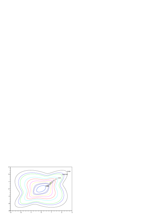
Figure 3: Level lines of the density function of the pair $(X,Y)$ defined in Example 2.

However, a proper limiting distribution can be obtained for $(X,Y)$ conditioned to remain in $\mathcal{C}=\{(x,y)\in\mathbb{R}^{2}\mid c_{1}x\leq y\leq c_{2}x\}$ for $c_{1}<c_{2}$ such that $\rho\in[c_{1},c_{2}]$ and $\tau\notin[c_{1},c_{2}]$. Denote $\mathbb{P}(\cdot\mid(X,Y)\in\mathcal{C})$ by $\mathbb{P}_{\mathcal{C}}(\cdot)$. Then

$$\lim_{x\to\infty}\mathbb{P}_{\mathcal{C}}(Y\leq\rho x+\sqrt{1-\rho^{2}}z\mid X>x)=\Phi(z)\;.$$ (10)

To prove this claim, we assume without loss of generality that $\rho=0$. Then

$$\mathbb{P}_{\mathcal{C}}(Y\leq z\mid X>x)=\frac{\mathbb{P}(Y\leq z\;;\ (X,Y)\in\mathcal{C}\mid X>x)}{\mathbb{P}((X,Y)\in\mathcal{C}\mid X>x)}\;.$$

For fixed $z$ and $x>z/c_{2}$, it holds that

$$\mathbb{P}(Y \leq z\;;\ (X,Y)\in\mathcal{C}\mid X>x)$$

$$=p\,\mathbb{P}(c_{1}X\leq Z\leq z\mid X>x)$$

$$\ \ \ +(1-p)\mathbb{P}(c_{1}X\leq\tau X+\sqrt{1-\tau^{2}}Z\leq z\mid X>x)\sim p\Phi(z)\;.$$

Since $\rho\in[c_{1},c_{2}]$ and $\tau\notin[c_{1},c_{2}]$, and since $z\leq c_{2}x$, it is easily obtained that

$$\lim_{x\to\infty}\mathbb{P}(c_{1}X\leq Z\leq z\mid X>x)=\Phi(z)\;,$$

$$\lim_{x\to\infty}\mathbb{P}(c_{1}X\leq\tau X+\sqrt{1-\tau^{2}}Z\leq z\mid X>x)=0\;.$$

Thus $\lim_{x\to\infty}\mathbb{P}(Y\leq z\;;\ (X,Y)\in\mathcal{C}\mid X>x)=p\Phi(z)$, which proves (10).

3 Bivariate vectors with polar representation

In this section, we show that Theorem 1 can be extended from elliptical distributions to more general bivariate distributions that admit a radial representation $R(u(T),v(T))$ where $R$ and $T$ are independent, $T$ is not uniformly distributed and $u$ and $v$ are more general functions than in the elliptical case. We start by collecting the assumptions that will be needed.

Assumption 2.

1. The function $u:[0,1]\to[0,1]$ is continuous, has a unique maximum 1 at a point $t_{0}\in(0,1)$ and has an expansion

   $$u(t_{0}+t)=1-\ell(t)$$ (11)

   where $\ell$ is decreasing from $[-\epsilon,0]$ to $[0,\eta_{-}]$ and increasing from $[0,\epsilon]$ to $[0,\eta_{+}]$ for some $\epsilon,\eta_{-},\eta_{+}>0$, and regularly varying at zero with index $\kappa>0$. The functions $\ell^{\leftarrow}_{-}:[0,\eta_{-}]\to[-\epsilon,0]$ and $\ell^{\leftarrow}_{+}:[0,\eta_{+}]\to[0,\epsilon]$ respectively defined as $\ell^{\leftarrow}_{-}(s)=\sup\{t\in[-\epsilon,0]:l(t)\leq s\}$ and $\ell^{\leftarrow}_{+}(s)=\inf\{t\in[0,\epsilon]:l(t)\geq s\}$ are absolutely continuous and their derivatives $(\ell^{\leftarrow}_{-})^{\prime}(s)$ and $(\ell^{\leftarrow}_{+})^{\prime}(s)$ are regularly varying at zero with index $1/\kappa-1$.

2. The function $v$ defined on $[0,1]$ is strictly increasing in a neighborhood of $t_{0}$, $v(t_{0})=\rho$, and the function $t\mapsto v(t_{0}+t)-\rho$ is regularly varying with index $\delta>0$. Its inverse $v^{\leftarrow}$ is absolutely continuous and its derivative is regularly varying at zero with index $1/\delta-1$.

Assumption 3.

The density function $g:[0,1]\to\mathbb{R}^{+}$ is regularly varying at $t_{0}$ with index $\tau>-1$ and bounded on the compact subsets of $[0,1]\setminus\{t_{0}\}$.

Theorem 3.

Let $R$ be in the domain of attraction of the Gumbel law with auxiliary function $\psi$, i.e. its distribution function $H$ satisfies (2). Let $T$ be a random variable that admits a density $g$ that satisfies Assumption 3. Let the functions $u$ and $v$ satisfy Assumption 2 with $\delta<\kappa$. Define $(X,Y)=R(u(T),v(T))$. Then,

1. the random variable $X$ is in the domain of attraction of the Gumbel law and there exists a function $k$ regularly varying at zero with index $(1+\tau)/\kappa$ such that

   $$\mathbb{P}(X>x)\sim k(\psi(x)/x)\bar{H}(x)\;;$$ (12)

2. there exists a function $h$ regularly varying at zero with index $\delta/\kappa$ such that for all $y\in\mathbb{R}$,

   $$\lim_{t\to\infty}\mathbb{P}(X\leq t+\psi(t)x\;,Y\leq\rho t+th(\psi(t)/t)y\mid X>t)\\ =(1-\mathrm{e}^{-x})H_{\kappa/\delta,(1+\tau)/\delta}(y)\;,$$ (13)

   with

   $$H_{\eta,\zeta}(y)=\frac{\int_{-\infty}^{y}\mathrm{e}^{-|s|^{\eta}/\eta}\,|s|^{\zeta-1}\,\mathrm{d}s}{\int_{-\infty}^{\infty}\mathrm{e}^{-|s|^{\eta}/\eta}\,|s|^{\zeta-1}\,\mathrm{d}s}\;.$$

The proof of this result is in Section 4. One of its main ingredient is the fact that the tail of $R$ is $\Gamma$-varying. This implies that the normalizing function $a(x)=xh(\psi(x)/x)$ is $o(x)$. As a consequence, only the local behavior of $u$ and $v$ around $(1,\rho)$ matters. This is similar to what was observed under Assumption 1.

Comments on Theorem 3

1. The case $u(t)=\cos(t)$ and $v(t)=\sin(t)$ was considered by Hashorva (2008). The difference between the present results and this reference is not only that we consider more general functions $u$ and $v$, but more importantly that we point out the local nature of the assumptions on $u$ and $v$.

2. Theorem 3 handles situations where the assumptions of Theorem 2 do not hold. In some cases, the limiting distribution is nevertheless the Gaussian distribution and the normalization is the same as in Theorem 3; see Example 3. In other cases, the limiting distribution and the normalization differ from those that appear in Theorem 2. There are two reasons for this: the density of $T$ can vanish or be unbounded at zero, or the curvature of the line parameterized by the functions $u$ and $v$ at the point $(u(t_{0}),v(t_{0}))$ can be infinite or zero. This is illustrated in Example 4.

   The asymptotic distribution $H_{\kappa/\delta,(1+\tau)/\delta}$ is of the so-called Weibull type with shape parameter $\kappa/\delta$. This ratio characterizes the geometric nature of the curve $t\mapsto(u(t),v(t))$ around $t_{0}$ and is independent of the particular choice of the parametrization $t\mapsto(u(t),v(t))$. Its right tail is lighter than the exponential distribution. The behavior of the density of $T$ has influence only on the less important parameter $\zeta$. The normalizing function $h$ also depends only on $u$ and $v$.

3. Denote $a(x)$ the normalizing function in (13): $a(x)=xh(\psi(x)/x)$. The assumption $\delta<\kappa$ implies that $\psi(x)=o(a(x))$, so that $(X-x)/a(x)$ converges weakly to zero given that $X>x$ as $x\to\infty$. Hence

   $$\lim_{x\to\infty}\mathbb{P}\left(\frac{Y-\rho X}{a(x)}\leq y\mid X>x\right)=H_{\kappa/\delta,(1+\tau)/\delta}(y)\;.$$

   This implies in particular that the case $\rho\neq 0$ can be deduced from the case $\rho=0$ by a linear transformation.

   Since the function $h$ is regularly varying with index $\delta/\kappa>0$ and since $\psi$ is self-neglecting, it also holds that $a(X)/a(x)$ converges weakly to 1 given that $X>x$ as $x\to\infty$, thus the conditional convergence also holds with random normalization:

   $$\lim_{x\to\infty}\mathbb{P}\left(\frac{Y-\rho X}{a(X)}\leq y\mid X>x\right)=H_{\kappa/\delta,(1+\tau)/\delta}(y)\;.$$

   This is a particular case of Heffernan and Resnick (2007, Proposition 5).

4. Note that Theorem 3 states that $X$ is in the domain of attraction of the Gumbel law, with the same auxiliary function $\psi$ as $R$. However, little can be said about the tails of $Y$ other than $\mathbb{P}(Y>y)\leq\mathbb{P}(R>y/v^{*})$, where $v^{*}=\max_{t\in[0,1]}v(t)$. This is because nothing is assumed about of the behaviour of $v$ and $g$ around the point where $v$ has a maximum. This would be needed to obtain an asymptotic form for the tail of $Y$ similar to (12). It is in contrast with the situation of Theorems 1 and 2. Nevertheless, it can first be proved that

   $$b_{Y}(t)\sim v^{*}b(t)$$ (14)

   where $b$ and $b_{Y}$ are the inverse functions of $1/\mathbb{P}(R>\cdot)$ and $1/\mathbb{P}(Y>\cdot)$, respectively (see a proof in Section 5). This implies that if $Y$ does belong to the domain of attraction of an extreme value distribution, then this distribution is necessarily the Gumbel law (since $Y$ has a lighter tail than $v^{*}R$ and unbounded support) and $(X,Y)$ belongs to the domain of attraction of a bivariate extreme value distribution with independent marginals, i.e. $X$ and $Y$ are asymptotically independent. This is shown in Corollary 5 below.

3.1 Relations with CEV and EV models

As mentioned in the introduction, Das and Resnick (2008) referred as CEV models the families of distributions satisfying Condition (1). An important finding of Heffernan and Resnick (2007) is that in such a model, it is not possible to transform $X$ and $Y$ to prescribed marginals $F_{1}(X)$ and $F_{2}(Y)$, for given univariate cdf $F_{1},F_{2}$, when the limiting distribution $K$ is the product of its marginals. Theorem 3 provides random vectors $(X,Y)$ for which the limiting distribution in (1) is precisely a product, so that nonlinear transformations of the marginals to prescribed marginals are impossible. This is in contrast with the usual practice of standard multivariate extreme value theory.

As noted by Das and Resnick (2009, Section 1.2), another advantage of the CEV approach is that it does not require the assumption that all components of the vector belong to the domain of attraction of a univariate extreme value distribution. The relationship between CEV models and EV models has been investigated in Das and Resnick (2008). They proved in particular that if $(X,Y)$ belongs to the domain of attraction of a bivariate extreme value distribution with asymptotic dependence, then the CEV model does not provide any more information than the EV model. See also Das and Resnick (2009, Section 1.2). Conversely, Das and Resnick (2009, Proposition 4.1) gives conditions under which, if $(X,Y)$ satisfies (1) and $Y$ belongs to the domain of attraction of a univariate extreme value distribution, then $(X,Y)$ belongs to the domain of attraction of a bivariate extreme value.

The next result elucidates the relationship between the conditional limit of Theorem 3 and extreme value theory. It is similar to Das and Resnick (2008, Proposition 4.1) but covers cases ruled out by this reference, as shown afterwards in Corollary 5. In the following, the extreme value distribution with index $\gamma$ is denoted by $G_{\gamma}$, that is to say $G_{\gamma}(y)=\exp\{-(1+\gamma y)^{-1/\gamma}\}$ for each $y$ such that $1+\gamma y>0$ for $\gamma\neq 0$, and $G_{0}(y)=\exp\{-e^{-x}\}$.

Proposition 4.

Assume that the vector $(X,Y)$ satisfies (1) and that $Y$ belongs to the domain of attraction of an extreme value distribution $G_{\gamma}$ with auxiliary function $\psi_{Y}$, i.e.

$$\lim_{t\to\infty}\mathbb{P}(Y>t+\psi_{Y}(t)y\mid Y>t)=-\log G_{\gamma}(y)\;.$$

Assume moreover that for all $y\in\mathbb{R}$,

$$\lim_{t\to\infty}\frac{b_{Y}(t)-m\circ b_{X}(t)+\psi_{Y}\circ b_{Y}(t)y}{a\circ b_{X}(t)}=+\infty\;$$ (15)

where $b_{X}$ and $b_{Y}$ are the inverse functions of $1/\mathbb{P}(X>\cdot)$, of $1/\mathbb{P}(Y>\cdot)$, respectively. Then, $(X,Y)$ belongs to the domain of attraction of a bivariate extreme value distribution with independent marginals, i.e. $X$ and $Y$ are asymptotically independent.

Proof.

To prove asymptotic independence, we must show that

$$\lim_{t\to\infty}t\mathbb{P}(X >b_{X}(t)+\psi\circ b_{X}(t)x\;,\;Y>b_{Y}(t)+\psi_{Y}\circ b_{Y}(t)y)=0\;,$$ (16)

where $\psi$ is as in (1). For any $y\in\mathbb{R}$, define $\tilde{y}$ by $b_{Y}(t)+\psi_{Y}\circ b_{Y}(t)y=m\circ b_{X}(t)+a\circ b_{X}(t)\tilde{y}$, i.e.

$$\tilde{y} =\frac{b_{Y}(t)-m\circ b_{X}(t)+\psi_{Y}\circ b_{Y}(t)y}{a\circ b_{X}(t)}\;.$$

Thus, by (15), for any $z\in\mathbb{R}$, we have,

$$\limsup_{t\to\infty} \;t\mathbb{P}(X>b_{X}(t)+\psi\circ b_{X}(t)x\;,\;Y>b_{Y}(t)+\psi_{Y}\circ b_{Y}(t)y)$$

$$=\limsup_{t\to\infty}\;t\mathbb{P}(X>b_{X}(t)+\psi\circ b_{X}(t)x\;,\;Y>m\circ b_{X}(t)+a\circ b_{X}(t)\tilde{y})$$

$$\leq\limsup_{t\to\infty}t\mathbb{P}(X>b_{X}(t)+\psi\circ b_{X}(t)x\;,\;Y>m\circ b_{X}(t)+a\circ b_{X}(t)z)$$

$$=\mathbb{P}(X^{*}>x\;,\ Y^{*}>z)\;,$$

where $(X^{*},Y^{*})$ is a random vector with distribution $K$. This can be made arbitrarily small by choosing $z$ large enough, so (16) holds. ∎

A simple example is provided by the elliptical distributions with identical margins, for which one has: $b_{X}=b_{Y}$, $\psi_{Y}(x)=o(x),\psi_{Y}(x)=o(a(x))$ and $m(x)=\rho x$, so that (15) holds. A more general result is provided by the following corollary.

Corollary 5.

Under the assumptions of Theorem 3, if moreover $Y$ belongs to a domain of attraction, then it is the Gumbel law, and (15) holds, so that $X$ and $Y$ are asymptotically independent.

Proof.

Under the assumptions of Theorem 3, the normalizing functions in (1) satisfy $m(t)=\rho t$, $\psi(t)=o(a(t))$ and $a(t)=o(t)$. Since $R$ has unbounded support, then so has $Y$ and since $Y$ has lighter tails than $v^{*}R$, the max-domain of attraction of $Y$ can only be the Gumbel law. Thus it also holds that $\psi_{Y}(t)=o(t)$. By (14) we know that $b_{Y}(t)\sim v^{*}b(t)$ and (12) implies that $b_{X}(t)\sim b(t)$. Thus we have

$$\frac{b_{Y}(t)-m\circ b_{X}(t)+\psi_{Y}\circ b_{Y}(t)y}{a\circ b_{X}(t)}\sim\frac{(v^{*}-\rho)b(t)}{a\circ b_{X}(t)}.$$

The assumptions on $v$ imply that $v^{*}>\rho$, so

$$\lim_{t\to\infty}\frac{(v^{*}-\rho)b(t)}{a\circ b_{X}(t)}=\infty\;.$$

Thus (15) holds for all $y\in\mathbb{R}$. ∎

Remark

Das and Resnick (2008, Proposition 4.1) show the same result under a condition which can be expressed with the present notation as $\lim_{t\to\infty}\psi_{Y}\circ b_{Y}(t)/a\circ b_{X}(t)\in(0,\infty]$. Under the conditions of Theorem 3, if moreover $v$ and $g$ satisfy some smoothness assumptions around the maximum of $v$ similar to Assumptions 2A and 3, it can be shown that $\psi_{Y}\sim\psi$ and thus $\lim_{t\to\infty}\psi_{Y}\circ b_{Y}(t)/a\circ b_{X}(t)=0$, so that Das and Resnick (2008, Proposition 4.1) cannot be applied here.

3.2 Some applications of Theorem 3

We now give some examples of applications of Theorem 3.

Example 3.

If the density $g$ of the variable $T$ has a positive limit at $t_{0}$, then $\tau=0$. If $u$ is twice differentiable with $u^{\prime}(t_{0})=0$ and $u^{\prime\prime}(t_{0})\neq 0$, then $\kappa=2$ and if $v^{\prime}(0)>0$, then $\delta=1$. If these three conditions hold, the limiting distribution is the standard Gaussian and the normalization is $\sigma\sqrt{x\psi(x)}$. Figure 2 also illustrates this case. As will be shown in Section 3.3, this is actually a particular case of Theorem 2.

Example 4.

Hashorva et al. (2007) have introduced a generalisation of the elliptical distributions, which they called $L_{p}$-Dirichlet distributions for all $p>0$. We consider here the case $p>1$. Instead of being ellipses, the level lines of the density of these distributions have the following equation:

$$|x|^{p}+\frac{|y-\rho x|^{p}}{1-|\rho|^{p}}=1\;,$$ (17)

with $\rho\in(-1,1)$. See Figure 4. To simplify the discussion, we consider the case $\rho=0$. An admissible parametrization is given by $u(t)=(1-t^{p})^{1/p}$ and $v(t)=t$, which yields $\delta=1$ and $\kappa=p$. Thus, Assumption 1 does not hold except if $p=2$, which is the elliptical context. If the density of $T$ has a positive limit at zero, then $\tau=0$ and the cdf of the limiting distribution is then

$$H_{p,1}(y)=\frac{\int_{-\infty}^{y}\mathrm{e}^{-|s|^{p}/p}\,\mathrm{d}s}{2p^{1/p-1}\,\Gamma(1/p)}\;.$$

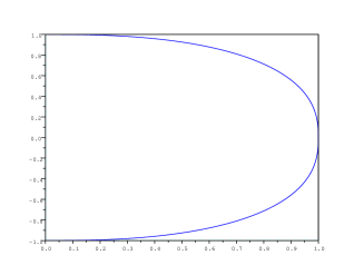
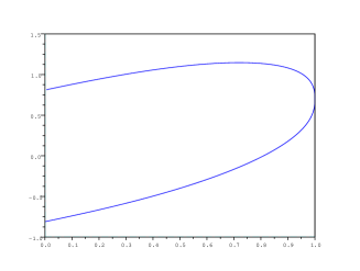
Figure 4: The curve given by Equation (17) with $p=3/2$, $\rho=0$ (left) and $\rho=.7$ (right).

As a last remark in this section, note that the result (12) on the upper tail of $X$ is actually a particular case of a more general result on the tail of the product of a random variable $X$ in the domain of attraction of the Gumbel law and a bounded random variable $U$. Similar results exist for heavy-tailed or subexponential distributions, for instance the celebrated Breiman’s Lemma (see Breiman (1965) and Cline and Samorodnitsky (1994)). In the present context, Hashorva (2008, Theorem 3) states a version of this result with $U=\cos\Theta$ and $\Theta$ has a density on $(-\pi,\pi)$. We state it under slightly more general assumptions which highlight the fact that only the behaviour of $U$ near its maximum must be specified.

Proposition 6.

Let $R$ be a nonnegative random variable whose cdf $H$ is in the domain of attraction of the Gumbel law. Let $U$ be a nonnegative random variable, independent of $R$, such that $U\leq b<\infty$ a.s. and that admits a density $g$ in a neighborhood of $b$ which is regularly varying at $b$ with index $\tau>-1$. Then $RU$ satisfies (2) with auxiliary function $\psi(x/b)$ and

$$\mathbb{P}(RU>x)\sim b^{2}\Gamma(\tau+1)\frac{\psi(x/b)}{x}\,g(\{1/b+\psi(x/b)/x\}^{-1})\bar{H}(x/b)\;.$$ (18)

Proof.

The proof is along the lines of the proof of (12), and makes use of Lemma 8. ∎

3.3 Relation between Theorems 2 and 3

Let $X,Y$ be random variables whose joint density $f$ can be expressed as

$$f(x,y)=g\circ n(x,y)\;,$$ (19)

where $g$ is a nonnegative function on $\mathbb{R}_{+}$ such that $\int_{0}^{\infty}rg(r)\,\mathrm{d}r<\infty$, $n$ is a positively homogeneous function with index 1 and the level line $n(x,y)=1$ admits the parametrization $t\to(u(t),v(t))$, $t\in[0,1]$. The change of variable $x=ru(t)$, $y=rv(t)$ yields, for any bounded measurable function $\varphi$:

$$\mathbb{E}[\varphi(X,Y)]=\int_{0}^{\infty}\int_{0}^{1}\varphi(ru(t),rv(t))\,rg(r)\,|u(t)v^{\prime}(t)-u^{\prime}(t)v(t)|\,\mathrm{d}r\,\mathrm{d}t\;.$$

Hence $(X,Y)=R(u(T),v(T))$, where $R$ has density $c(g)^{-1}rg(r)$, with $c(g)=\int_{0}^{\infty}rg(r)\,dr$ and $T$ has density $c(u,v)^{-1}|uv^{\prime}-u^{\prime}v|$ with $c(u,v)=\int_{0}^{1}|u^{\prime}(t)v(t)-u(t)v^{\prime}(t)|\mathrm{d}t$.

Conversely, if $(X,Y)=R(u(T),v(T))$ where $R$ and $T$ are independent, $R$ has a density $h$ on $[0,\infty)$, and if there exists a point $t_{0}$ such that $u^{\prime}(t_{0})=0$, $u^{\prime\prime}(t_{0})>0$ and $v^{\prime}(t_{0})>0$, then the function $v/u$ is invertible on an interval around $t_{0}$. Let $\phi$ be its inverse, and define $n(x,y)=x/\{u\circ\phi(y/x)\}$. Without loss of generality, we can assume that $u(t_{0})=1$ and denote $v(t_{0})=\rho$. Then $n$ is a positively homogeneous function with index 1, and if $T$ admits a density $g$, then $(X,Y)$ has a density $f$ in a cone $C=\{(x,y)\mid(\rho-\epsilon)x\leq y\leq(\rho+\epsilon)x\}$ around the line $y=\rho x$, defined by

$$f(x,y)=\frac{h(n(x,y))}{n(x,y)}\;L(x,y)\;,$$

with

$$L(x,y)=\frac{g\circ\phi(y/x)}{|u^{\prime}v-uv^{\prime}|\circ\phi(y/x)}\;.$$

If the density $g$ and the Jacobian $|u^{\prime}v-uv^{\prime}|$ are both positive and continuous at $t_{0}$, then the function $L$ belongs to the class ${\cal L}$. See Lemma 9 for a proof. Thus Assumption 1 locally holds, and Theorem 2 implies Theorem 3 in this context.

3.4 Second order correction

As illustrated in Abdous et al. (2008), it is useful for statistical purposes to have a second order correction to the asymptotic approximation (13) provided by Theorem 3. In order to obtain such a refinement, rates of convergence in all the approximations used to prove Theorem 3 are needed. To simplify the discussion, we will consider the following additional assumptions.

• The random variable $T$ is uniformly distributed over $[0,1]$.

• There exist $\lambda>0$ and $\sigma>0$ such that

  $$u(t_{0}+t)=1-\frac{\sigma^{2}t^{2}}{2}+o(t^{3})\;,\ \ v(t_{0}+t)=\rho+\lambda t+O(t^{2})\;.$$

• There exist functions $\chi$ and $B$ such that

  $$\left|\frac{\bar{H}(x+t\psi(x))}{\bar{H}(x)}-\mathrm{e}^{-t}\right|\leq\chi(x)B(t)\;,$$ (20)

  for all $t\geq 0$ and $x$ large enough, where $\lim_{x\to\infty}\chi(x)=0$, and $B$ is bounded on the compact subsets of $[0,\infty)$ and integrable over $[0,\infty)$.

The bound (20) is a nonuniform rate of convergence. See Abdous et al. (2008, section 2.2) for examples. Under these assumptions, it is possible to obtain a rate of convergence and a second order correction in Theorem 3. Proceeding as in the proof of Abdous et al. (2008, Theorem 3) yields

$$\mathbb{P}(Y\leq\rho x+\frac{\lambda}{\sigma}\sqrt{x\psi(x)}z\mid X>x)\\ =\Phi(z)-\frac{\rho}{\lambda}\sqrt{\frac{\psi(x)}{x}}\phi(z)+O(\chi(x))+o\left(\sqrt{\psi(x)/x}\right)\;.$$

Replacing $z$ by $z+\rho\lambda^{-1}\sqrt{\psi(x)/x}$ yields

$$\mathbb{P}\left(Y\leq\rho x+\frac{\lambda}{\sigma}\sqrt{x\psi(x)}z+\frac{\rho}{\sigma}\psi(x)\mid X>x\right)\\ =\Phi(z)+O(\chi(x))+o\left(\sqrt{\psi(x)/x}\right)\;.$$

This second order correction is meaningful only if $\chi(x)=o(\sqrt{\psi(x)})$. The improvement is only moderate here: the bound is $o(\sqrt{\psi(x)/x})$ instead of $O(\sqrt{\psi(x)/x})$, because we assumed only that $u(t_{0}+t)=1-\sigma^{2}t^{2}/2+o(t^{3})$. If the expansion of $u$ around $t_{0}$ is $u(t_{0}+t)=1-\sigma^{2}t^{2}/2+O(t^{4})$, then the bound becomes $O(\psi(x)/x)$. This is the case for bivariate elliptical distributions.

4 Proof of Theorem 3

Let $\epsilon$ be defined as in Assumption 2. Since $u$ has its maximum at $t_{0}$, there exists $\eta>0$ such that for all $t\notin[t_{0}-\epsilon,t_{0}+\epsilon]$, it holds that $u(t)\leq 1-\eta$. Then,

$$\mathbb{P}(X>x\;;\ Y>y) =\int_{0}^{1}\bar{H}\left(\frac{x}{u(t)}\vee\frac{y}{v(t)}\right)g(t)\,\mathrm{d}t$$

$$=\int_{|t-t_{0}|\leq\epsilon}\bar{H}\left(\frac{x}{u(t)}\vee\frac{y}{v(t)}\right)g(t)\,\mathrm{d}t$$

$$+\int_{|t-t_{0}|>\epsilon}\bar{H}\left(\frac{x}{u(t)}\vee\frac{y}{v(t)}\right)g(t)\,\mathrm{d}t\;.$$

Let $r(x)$ denote the last term. The bound (22) in Lemma 7 yields that for any $p>0$,

$$r(x)\leq\bar{H}(x/(1-\eta))=O\left(\{\psi(x)/x\}^{p}\bar{H}(x)\right)\;.$$

This will prove that $r(x)$ is negligible with respect to the first integral for which we now give an asymptotic equivalent. By assumption, we can choose $\epsilon$ such that the function $v/u$ is continuous and increasing on $[t_{0}-\epsilon,t_{0}+\epsilon]$, because $\delta<\kappa$, so that $v/u\sim v$ in a neighborhood of $t_{0}$.

If $y$ can be expressed as $y=\rho x+o(x)$, then for large $x$, it holds that $y/x\in[(v/u)(t_{0}-\epsilon),(v/u)(t_{0}+\epsilon)]$. If $y/x>\rho=(v/u)(t_{0})$, then there exists $t_{1}\in[t_{0},t_{0}+\epsilon]$ such that $(v/u)(t_{1})=y/x$. Thus,

$$\int_{t_{0}-\epsilon}^{t_{0}+\epsilon}\bar{H}\left(\frac{x}{u(t)}\vee\frac{y}{v(t)}\right)g(t)\,\mathrm{d}t\\ =\int_{t_{0}-\epsilon}^{t_{1}}\bar{H}\left(\frac{y}{v(t)}\right)g(t)\,\mathrm{d}t+\int_{t_{1}}^{t_{0}+\epsilon}\bar{H}\left(\frac{x}{u(t)}\right)g(t)\,\mathrm{d}t\;.$$

Let $I$ and $J$ denote the last two integrals, respectively. The successive changes of variables $s=1/u(t)$ and $s=1+\omega\psi(x)/x$ yield

$$J=\int_{1/u(t_{1})}^{1/u(t_{0}+\epsilon)}\bar{H}(xs)\frac{-(u^{\leftarrow})^{\prime}(1/s)}{s^{2}}g(u^{\leftarrow}(1/s))\,\mathrm{d}s\\ =\frac{\psi(x)}{x}\int_{x\{1/u(t_{1})-1\}/\psi(x)}^{x\{1/u(t_{0}+\epsilon)-1\}/\psi(x)}\bar{H}(x+\psi(x)\omega)\\ \times\frac{-(u^{\leftarrow})^{\prime}(1/\{1+\omega\psi(x)/x\})}{\{1+\omega\psi(x)/x\}^{2}}g(u^{\leftarrow}(1/\{1+\omega\psi(x)/x\}))\,\mathrm{d}\omega\;.$$

Let $k_{1}$ denote the function defined by

$$k_{1}(\omega)=-\omega(u^{\leftarrow})^{\prime}(1/\{1+\omega\})g(u^{\leftarrow}(1/\{1+\omega\}))\;.$$

Assumptions 2 and 3 imply that $k_{1}$ is regularly varying at zero with index $(1+\tau)/\kappa$ and Lemma 8 yields

$$J\sim k_{1}\{\psi(x)/x\}\bar{H}(x)\int_{z_{0}}^{\infty}\mathrm{e}^{-t}t^{(1+\tau)/\kappa-1}\,\mathrm{d}t\;,$$

where $z_{0}=x\{1/u(t_{1})-1\}/\psi(x)$ and if $y$ is chosen in such a way that $z_{0}$ has a finite limit when $x\to\infty$. Set $y/x=\rho+\xi$. Then, by definition of $t_{1}$, $z_{0}=x\{1/u\circ(v/u)^{\leftarrow}(\rho+\xi)-1\}/\psi(x)$. Assumption 2 implies that the function $\xi\mapsto u\circ(v/u)^{\leftarrow}(\rho+\xi)$ is regularly varying at zero with index $\kappa/\delta$. Define an increasing function $h$ which is regularly varying at zero with index $\delta/\kappa$ by

$$h(x)=(v/u)\circ u^{\leftarrow}(1/\{1+x\})-\rho=(1+x)v\circ u^{\leftarrow}(1/\{1+x\})-\rho\;.$$

For $z\geq 0$, set $y/x=\rho+h(\psi(x)/x)z$. Then

$$z_{0}=\frac{x}{\psi(x)}h^{\leftarrow}(h(\psi(x)/x)z)\sim z^{\kappa/\delta}\;,$$

$$J\sim k_{1}\{\psi(x)/x\}\bar{H}(x)\int_{z^{\kappa/\delta}}^{\infty}\mathrm{e}^{-t}t^{(1+\tau)/\kappa-1}\,\mathrm{d}t\;.$$

We next deal with the integral $I$, still in the case $y/x>\rho$. Noting that $\{y/v(t_{1})-x\}/\psi(x)=z_{0}$, the changes of variables $s=1/v(t)$ and $s=\{x+\psi(x)\omega)\}/y$ yield

$$I =\int_{1/v(t_{1})}^{1/v(t_{0}-\epsilon)}\bar{H}(ys)\frac{(v^{\leftarrow})^{\prime}(1/s)}{s^{2}}g(v^{\leftarrow}(1/s))\,\mathrm{d}s$$

$$=\frac{y\psi(x)}{x^{2}}\int_{z_{0}}^{\{y/v(t_{0}-\epsilon)-x\}/\psi(x)}\bar{H}(x+\psi(x)\omega)$$

$$\phantom{\frac{y\psi(x)}{x^{2}}}\times\frac{(v^{\leftarrow})^{\prime}((y/x)/\{1+\omega\psi(x)/x\})}{\{1+\omega\psi(x)/x\}^{2}}g(v^{\leftarrow}((y/x)/\{1+\omega\psi(x)/x\}))\mathrm{d}\omega\;.$$

The choice $y/x=\rho+h(\psi(x)/x)z$ also yields

$$\frac{y/x}{1+\omega\psi(x)/x} =\frac{\rho+h(\psi(x)/x)z}{1+\omega\psi(x)/x}\sim\rho+h(\psi(x)/x)z\;.$$

Let the function $k_{2}$ be defined by

$$k_{2}(\xi)=\xi(v^{\leftarrow})^{\prime}(\rho+h(\xi))g\circ v^{\leftarrow}(\rho+h(\xi))\;.$$

Assumptions 2 and 3 imply that $k_{2}$ is regularly varying at zero with index $(1+\tau)/\kappa+1-\delta/\kappa>(1+\tau)/\kappa$. Lemma 8 yields

$$I\sim\rho z^{(1+\tau)/\delta-1}k_{2}(\psi(x)/x)\bar{H}(x)\int_{z^{\kappa/\delta}}^{\infty}\mathrm{e}^{-t}\,\mathrm{d}t=o(J)\;.$$

The case $y/x<\rho$ can be dealt with similarly and is omitted. The remaining of the proof of assertions (i) and (ii) is straightforward. ∎

5 Lemmas

The following Lemma is a straightforward consequence of the representation theorem for the class $\Gamma$ (Bingham et al., 1989, Theorem 3.10.8). The argument was used in the proof of Abdous et al. (2005, Theorem 1). We briefly recall the main lines of the proof for the sake of completeness.

Lemma 7.

Let $H$ be a cdf in the domain of attraction of the Gumbel law infinite right endpoint. For any $p>0$, there exists a constant $C$ such that for all $x$ large enough, and all $t\geq 0$,

$$\frac{\bar{H}(x+\psi(x)t)}{\bar{H}(x)}\leq C(1+t)^{-p}\;.$$ (21)

$$\frac{\bar{H}(\alpha x)}{\bar{H}(x)}\leq C(\psi(x)/x)^{p}\;.$$ (22)

Proof.

If $\gamma=0$, the function $\bar{H}$ can be expressed as

$$\bar{H}(x)=c(x)\exp\left\{-\int_{x_{0}}^{x}\frac{\mathrm{d}s}{\psi(x)}\right\}$$

where $\lim_{x\to\infty}c(x)=c\in(0,\infty)$ and $\lim_{x\to\infty}\psi^{\prime}(x)=0$. Thus, for any $\epsilon>0$ and $x$ large enough, there exists a constant $C$ such that

$$\frac{c(x+\psi(x)t)}{c(x)}\leq C\;,\ \ \ \frac{\psi(x+\psi(x)t)}{\psi(x)}\leq 1+\epsilon t\;.$$

Hence

$$\frac{\bar{H}(x+\psi(x)t)}{\bar{H}(x)} \leq C\exp\left\{-\int_{0}^{t}\frac{\mathrm{d}s}{1+\epsilon s}\right\}=C(1+\epsilon t)^{-1/\epsilon}\;.$$

This proves (21). The bound (22) follows trivially from (21) by choosing $\epsilon<1/p$ and by setting $t=(\alpha-1)x/\psi(x)$. ∎

Lemma 8.

Let $H$ be a cdf in the domain of attraction of the Gumbel law with infinite right endpoint. Let $g$ be a function regularly varying at zero with index $\tau>-1$ and bounded on compact subsets of $(0,\infty]$. Then

$$\lim_{x\to\infty}\int_{z}^{\infty}\frac{\bar{H}(x+\psi(x)t)}{\bar{H}(x)}\frac{g(t\psi(x)/x)}{g(\psi(x)/x)}\,\mathrm{d}t=\int_{z}^{\infty}t^{\tau}\,\mathrm{e}^{-t}\,\mathrm{d}t\;,$$

locally uniformly with respect to $z\geq 0$.

Proof.

Denote $\chi(x)=\psi(x)/x$; then $\lim_{x\to\infty}\chi(x)=0$. By assumption, $\bar{H}(x+\psi(x)t)/\bar{H}(x)$ converges to $\mathrm{e}^{-t}$ and $g(\chi(x)t)/g(\chi(x))$ converges to $t^{\tau}$, and both convergences are uniform on compact sets of $(0,\infty)$. It is thus sufficient to prove that

$$\lim_{A\to\infty}\limsup_{x\to\infty}\int_{A}^{\infty}\frac{\bar{H}(x+\psi(x)t)}{\bar{H}(x)}\frac{g(\chi(x)t)}{g(\chi(x))}\,\mathrm{d}t=0\;,$$ (23)

$$\lim_{\eta\to 0}\limsup_{x\to\infty}\int_{0}^{\eta}\frac{\bar{H}(x+\psi(x)t)}{\bar{H}(x)}\frac{g(\chi(x)t)}{g(\chi(x))}\,\mathrm{d}t=0\;.$$ (24)

Let $\epsilon>0$ be such that $1/\epsilon-1>\tau$. By Lemma 7, for large enough $x$,

$$\int_{A}^{\infty}\frac{\bar{H}(x+\psi(x)t)}{\bar{H}(x)}g(\chi(x)t)\,\mathrm{d}t \leq C\int_{A}^{\infty}t^{-1/\epsilon}g(\chi(x)t)\,\mathrm{d}t$$

$$=C\chi(x)^{1/\epsilon-1}\int_{A\chi(x)}^{\infty}t^{-1/\epsilon}g(t)\,\mathrm{d}t\;.$$

Since $g$ is locally bounded on $(0,\infty]$ and $-1/\epsilon+\tau<-1$, Karamata’s Theorem (cf. for instance Bingham et al. (1989, Proposition 1.5.10)) implies that there exists a constant $C^{\prime}$ such that

$$\int_{A\chi(x)}^{\infty}t^{-1/\epsilon}g(t)\,\mathrm{d}t \leq C^{\prime}(\chi(x)A)^{1-1/\epsilon}g(\chi(x)A)\;,$$

$$\limsup_{x\to\infty}\int_{A}^{\infty}\frac{\bar{H}(x+\psi(x)t)}{\bar{H}(x)}\frac{g(\chi(x)t)}{g(\chi(x))}\,\mathrm{d}t \leq CC^{\prime}A^{1-1/\epsilon}\limsup_{x\to\infty}\frac{g(\chi(x)A)}{g(\chi(x))}$$

$$=CC^{\prime}A^{1-1/\epsilon+\tau}\to 0$$

as $A$ tends to infinity, because $1-1/\epsilon+\tau<0$. This proves (23). Since $\bar{H}(x+\psi(x)t)/\bar{H}(x)\leq 1$ and by Karamata’s Theorem, we get, for some constant $C$,

$$\int_{0}^{\eta}\frac{\bar{H}(x+\psi(x)t)}{\bar{H}(x)}g(\chi(x)t)\,\mathrm{d}t \leq\int_{0}^{\eta}g(\chi(x)t)\,\mathrm{d}t$$

$$=\chi(x)^{-1}\int_{0}^{\chi(x)\eta}g(t)\,\mathrm{d}t\leq C\eta g(\chi(x)\eta)\;.$$

Hence

$$\lim_{\eta\to 0}\limsup_{x\to\infty}\int_{0}^{\eta}\frac{\bar{H}(x+\psi(x)t)}{\bar{H}(x)}\frac{g(\chi(x)t)}{g(\chi(x))}\,\mathrm{d}t\leq\lim_{\eta\to 0}C\eta^{1+\tau}=0\;,$$

because $1+\tau>0$, which proves (24). ∎

Lemma 9.

Let $\ell$ be a continuous function defined on $[0,\infty)$, bounded above and away from zero and with a finite limit at infinity. Define $L$ on $\mathbb{R}_{+}\times\mathbb{R}_{+}$ by $L(x,y)=\ell(y/x)$. Then $L$ belongs to the class $\mathcal{L}$.

Proof.

Since $\ell$ is bounded, it suffices to prove that if the limit $\lim_{(\xi,\zeta)\to\infty}\ell((x+\xi)/(y+\zeta))/\ell(\xi/\zeta)$ exists, then it is equal to 1. Since moreover $\ell$ is continuous and bounded away from zero, it is enough to consider subsequences and to show that if $\|(\xi_{n},\zeta_{n})\|\to\infty$ and if $\lim_{n\to\infty}\xi_{n}$ and $\lim_{n\to\infty}\zeta_{n}$ both exist, then $\lim_{n\to\infty}(x+\xi_{n})/(y+\zeta_{n})=\lim_{n\to\infty}\xi_{n}/\zeta_{n}$. Three cases arise.

1. If $\lim_{n\to\infty}\xi_{n}=\lim_{n\to\infty}\zeta_{n}=\infty$, then

   $$\frac{x+\xi_{n}}{y+\zeta_{n}}=\frac{\xi_{n}}{\zeta_{n}}\,\frac{1+x/\xi_{n}}{1+y/\zeta_{n}}\sim\xi_{n}/\zeta_{n}\;.$$

2. If $\lim_{n\to\infty}\xi_{n}<\infty$ and $\lim_{n\to\infty}\zeta_{n}=\infty$, then

   $$\lim_{n\to\infty}(x+\xi_{n})/(y+\zeta_{n})=0=\lim_{n\to\infty}\xi_{n}/\zeta_{n}\;.$$

3. If $\lim_{n\to\infty}\xi_{n}=\infty$ and $\lim_{n\to\infty}\zeta_{n}<\infty$, then

   $$\lim_{n\to\infty}(x+\xi_{n})/(y+\zeta_{n})=\infty=\lim_{n\to\infty}\xi_{n}/\zeta_{n}\;.$$

∎

Proof of (14).

By assumption, $\mathbb{P}(Y>y)\leq\bar{H}(y/v^{*})$, thus $b_{Y}(t)\leq v^{*}b(t)$. Denote $V=v(T)$. Two cases only are possible: (i) $v^{*}$ is an isolated point of the support of the distribution of $V$ and $\mathbb{P}(V=v^{*})>0$; (ii) $\mathbb{P}(V=v*)=0$ and for any $\epsilon>0$, there exists $v\in(v^{*}-\epsilon,v^{*})$ such that $\mathbb{P}(V>v)>0$.

1. If $\mathbb{P}(V=v^{*})>0$ and $v^{*}$ is an isolated point, then there exists $v^{**}<v^{*}$ such that

   $$\mathbb{P}(Y>y)=\bar{H}(y/v^{*})\mathbb{P}(V=v^{*})+\mathbb{P}(RV>y\;,\;V\leq v^{**})\;.$$

   Note that $\mathbb{P}(RV>y\;,\;V\leq v^{**})\leq\bar{H}(y/v^{**})$, and since $\bar{H}$ is $\Gamma$-varying, $\bar{H}(y/v^{**})=o(\bar{H}(y/v^{*}))$, thus $\mathbb{P}(Y>y)\sim\epsilon\bar{H}(y/v^{*})$ with $\epsilon=\mathbb{P}(V=v^{*})$. Since $b$ is slowly varying, this implies that $b_{Y}(t)\sim v^{*}b(\epsilon t)$ and finally that $b_{Y}(t)\sim v^{*}b(t)$ as $t\to\infty$.

2. In the second case, fix some $v<v*$ and denote $\epsilon=\mathbb{P}(V>v)>0$ by assumption. Then

   $$\mathbb{P}(Y>y) =\mathbb{P}(RV>y\;,\;V>v)+\mathbb{P}(RV>y\;,\;V\leq v)\geq\epsilon\mathbb{P}(R>y/v).$$

   Thus, $b_{Y}(t)\geq vb(\epsilon t)$ and since $b$ is slowly varying,

   $$\liminf_{t\to\infty}\frac{b_{Y}(t)}{b(t)}\geq v\;.$$

   Since $v$ can be chosen arbitrarily close to $v^{*}$ and since we already know that $b_{Y}(t)\leq v^{*}b(t)$, we conclude that $\lim_{t\to\infty}b_{Y}(t)/b(t)=v^{*}$.

∎

Acknowledgement

We thank the associate editor and the referees for their comments and suggestions that helped to substantially improve our paper.

References

- Abdous et al. (2005) Belkacem Abdous, Anne-Laure Fougères, and Kilani Ghoudi. Extreme behaviour for bivariate elliptical distributions. Revue Canadienne de Statistiques, 33(2):1095–1107, 2005.
- Abdous et al. (2008) Belkacem Abdous, Anne-Laure Fougères, Kilani Ghoudi, and Philippe Soulier. Estimation of bivariate excess probabilities for elliptical models. Bernoulli, 14(4):1065–1088, 2008.
- Balkema and Embrechts (2007) Guus Balkema and Paul Embrechts. High risk scenarios and extremes. A geometric approach. Zurich Lectures in Advanced Mathematics. Zürich: European Mathematical Society, 2007.
- Barbe (2003) Philippe Barbe. Approximation of integrals over asymptotic sets with applications to probability and statistics. http://arxiv.org/abs/math/0312132, 2003.
- Berman (1983) Simeon M. Berman. Sojourns and extremes of Fourier sums and series with random coefficients. Stochastic Processes and their Applications, 15(3):213–238, 1983.
- Berman (1992) Simeon M. Berman. Sojourns and extremes of stochastic processes. The Wadsworth & Brooks/Cole Statistics/Probability Series. Wadsworth & Brooks/Cole Advanced Books & Software, Pacific Grove, CA, 1992.
- Bingham et al. (1989) N. H. Bingham, C. M. Goldie, and J. L. Teugels. Regular variation, volume 27 of Encyclopedia of Mathematics and its Applications. Cambridge University Press, Cambridge, 1989.
- Breiman (1965) Leo Breiman. On some limit theorems similar to the arc-sin law. Theory of Probability and its Applications, 10:351–360, 1965.
- Cline and Samorodnitsky (1994) Daren B. H. Cline and Gennady Samorodnitsky. Subexponentiality of the product of independent random variables. Stochastic Process. Appl., 49(1):75–98, 1994.
- Das and Resnick (2008) Bikramjit Das and Sidney I. Resnick. Conditioning on an extreme component: Model consistency and regular variation on cones. http://arxiv.org/abs/0805.4373, 2008.
- Das and Resnick (2009) Bikramjit Das and Sidney I. Resnick. Detecting a conditional extrme value model. http://arxiv.org/abs/0902.2996, 2009.
- De Haan and Ferreira (2006) Laurens De Haan and Ana Ferreira. Extreme value theory. An introduction. Springer Series in Operations Research and Financial Engineering. New York, NY: Springer., 2006.
- Eddy and Gale (1981) William F. Eddy and James D. Gale. The convex hull of a spherically symmetric sample. Advances in Applied Probability, 13(4):751–763, 1981.
- Fougères and Soulier (2008) Anne-Laure Fougères and Philippe Soulier. Estimation of conditional laws given an extreme component. arXiv:0806.2426, 2008.
- Hashorva (2005) Enkelejd Hashorva. Extremes of asymptotically spherical and elliptical random vectors. Insurance: Mathematics & Economics, 36(3):285–302, 2005.
- Hashorva (2006) Enkelejd Hashorva. Gaussian approximation of conditional elliptic random vectors. Stoch. Models, 22(3):441–457, 2006.
- Hashorva (2008) Enkelejd Hashorva. Conditional limit results for type I polar distributions. Extremes, 10.1007/s10687-008-0078-y, 2008.
- Hashorva et al. (2007) Enkelejd Hashorva, Samuel Kotz, and Alfred Kume. -norm generalised symmetrised Dirichlet distributions. Albanian Journal of Mathematics, 1(1):31–56 (electronic), 2007.
- Heffernan and Resnick (2007) Janet E. Heffernan and Sidney I. Resnick. Limit laws for random vectors with an extreme component. Annals of Applied Probability, 17(2):537–571, 2007.
- Heffernan and Tawn (2004) Janet E. Heffernan and Jonathan A. Tawn. A conditional approach for multivariate extreme values. Journal of the Royal Statistical Society. Series B, 66(3):497–546, 2004.
- Resnick (2002) Sidney Resnick. Hidden regular variation, second order regular variation and asymptotic independence. Extremes, 5(4):303–336, 2002.
- Resnick (1987) Sidney I. Resnick. Extreme values, regular variation, and point processes, volume 4 of Applied Probability. A Series of the Applied Probability Trust. Springer-Verlag, New York, 1987.