The affine LIBOR models

Abstract.

We provide a general and flexible approach to LIBOR modeling based on the class of affine factor processes. Our approach respects the basic economic requirement that LIBOR rates are non-negative, and the basic requirement from mathematical finance that LIBOR rates are analytically tractable martingales with respect to their own forward measure. Additionally, and most importantly, our approach also leads to analytically tractable expressions of multi-LIBOR payoffs. This approach unifies therefore the advantages of well-known forward price models with those of classical LIBOR rate models. Several examples are added and prototypical volatility smiles are shown. We believe that the CIR-process based LIBOR model might be of particular interest for applications, since closed form valuation formulas for caps and swaptions are derived.

1. Introduction

Let $T_{0}<\ldots<T_{N}$ be a discrete tenor of maturity dates. LIBOR rates are related to the observable ratio of prices of zero-coupon bonds with maturity $T_{k-1}$ and $T_{k}=T_{k-1}+\delta$ via

$$L(t,T_{k-1})=\frac{1}{\delta}\left(\frac{B(t,T_{k-1})}{B(t,T_{k})}-1\right).$$

The nature of interbank loans, as well as the daily calculation of LIBOR rates as the trimmed arithmetic average of interbank quoted rates (see www.bbalibor.com), yield that LIBOR rates should be non-negative. A requirement from mathematical finance is that LIBOR rates should be martingales with respect to their own forward measure $\mathrm{I\kern-1.99997ptP}_{T_{k}}$. That is, when $B(\cdot,T_{k})$ is considered as numéraire of the model, then discounted bond prices $\big{(}\frac{B(t,T_{k-1})}{B(t,T_{k})}\big{)},{0\leq t\leq T_{k-1}}$ should be martingales. An additional basic requirement motivated by applications is the tractability of the model, since otherwise one cannot calibrate to the market data. Therefore the LIBOR rate processes $L(\cdot,T_{k-1})$ should have tractable stochastic dynamics with respect to their forward measure $\mathrm{I\kern-1.99997ptP}_{T_{k}}$, for $k=1,\ldots,N$; for instance of exponential Lévy type along the discrete tenor of dates $T_{0}<\ldots<T_{N}$. Here the terminus “analytically tractable” is used in the sense that either the density of the stochastic factors driving the LIBOR rate process is known explicitly, or the characteristic function. In both cases, the numerical evaluation, which is needed for calibration to the market, is easily done.

In applications, the stochastic factors have to be evaluated with respect to different numéraires. In order to describe the dynamics with respect to a suitable martingale measure, for instance the terminal forward measure $\mathrm{I\kern-1.99997ptP}_{T_{N}}$, we have to perform a change of measure. Usually this change of measure destroys the tractable structure of $L(\cdot,T_{k-1})$ with respect to its forward measure. This well-known phenomenon makes LIBOR market models based on Brownian motions or Lévy processes quite delicate to apply for multi-LIBOR-dependent payoffs: either one performs expensive Monte Carlo simulations or one has to approximate the equation (the keyword here is “freezing the drift”, see e.g. SiopachaTeichmann07).

In order to overcome this natural intractability, forward price models have been considered, where the tractability with respect to other forward measures is pertained when changing the measure. Hence, modeling forward prices $F(\cdot,T_{k-1},T_{k})=1+\delta L(\cdot,T_{k})$ produces a very tractable model class. However negative LIBOR rates can occur with positive probability, which contradicts any economic intuition.

In this work, we propose a new approach to modeling LIBOR rates based on affine processes. The approach follows the footsteps of forward price models, however, we are able to circumvent their drawback: in our approach LIBOR rates are almost surely non-negative. Moreover, the model remains analytically tractable with respect to all possible forward measures, hence the calibration and evaluation of derivatives is fairly simple. In fact, this is the first LIBOR model where the following are satisfied simultaneously:

• LIBOR rates are non-negative;

• caps and swaptions can be priced easily using Fourier methods, for several affine factor processes;

• closed-form valuation formulas for caps and swaptions are derived for the CIR process, in 1- and 2-factor models.

A particular feature of our approach is that the factor process is a time-homogenous Markov process when we consider the model with respect to the terminal measure $\mathrm{I\kern-1.99997ptP}_{T_{N}}$. With respect to forward measures the factor processes will show time-inhomogeneities due to the nature of the change of measure. When we compare our approach to an affine factor setting within the HJM-methodology, we observe that in both cases one can choose – with respect to the spot measure in the HJM setting or with respect to the terminal measure in our setting – a time-homogeneous factor process. LIBOR rates have in both cases a typical dependence on time-to-maturity $T_{N}-t$.

The remainder of the article is organized as follows: in Section 2 we formulate basic axioms for LIBOR market models. In Section 3 we recapitulate the literature on LIBOR models. In Section 4 we introduce affine processes which are applied in Section 5 to the construction of certain martingales. In Section 6 we present our new approach to LIBOR market models, which is applied in Section 7 to derivative pricing. In Section 8 several examples, including the CIR-based models, are presented and in Section 9 we show prototypical volatility surfaces generated by the models.

2. Axioms

Let us denote by $L(t,T)$ the time-$t$ forward LIBOR rate that is settled at time $T$ and received at time $T+\delta$; here $T$ denotes some finite time horizon. The LIBOR rate is related to the prices of zero coupon bonds, denoted by $B(t,T)$, and the forward price, denoted by $F(t,T,T+\delta)$, by the following equations:

$$1+\delta L(t,T)=\frac{B(t,T)}{B(t,T+\delta)}=F(t,T,T+\delta).$$ (2.1)

One postulates that the LIBOR rate should satisfy the following axioms, motivated by economic theory, arbitrage pricing theory and applications.

Axiom 1.

The LIBOR rate should be non-negative, i.e. $L(t,T)\geq 0$ for all $0\leq t\leq T$.

Axiom 2.

The LIBOR rate process should be a martingale under the corresponding forward measure, i.e. $L(\cdot,T)\in\mathcal{M}(\mathrm{I\kern-1.99997ptP}_{T+\delta})$.

Axiom 3.

The LIBOR rate process, i.e. the (multivariate) collection of all LIBOR rates, should be analytically tractable with respect to as many forward measures as possible. Minimally, closed-form or semi-analytic valuation formulas should be available for the most liquid interest rate derivatives, i.e. caps and swaptions, so that the model can be calibrated to market data in reasonable time.

Furthermore we wish to have rich structural properties: that is, the model should be able to reproduce the observed phenomena in interest rate markets, e.g. the shape of the implied volatility surface in cap markets or the implied correlation structure in swaption markets.

3. Existing approaches

There are several approaches to LIBOR modeling developed in the literature attempting to fulfill the axioms and practical requirements discussed in the previous section. We briefly describe below the two main approaches, namely the LIBOR market model (LMM) and the forward price model, and comment on their ability to fulfill them. We also briefly discuss Markov-functional models.

Approach 1.

In LIBOR market models, developed in a series of articles by SandmannSondermannMiltersen95, MiltersenSandmannSondermann97, BraceGatarekMusiela97, and Jamshidian97, each forward LIBOR rate is modeled as an exponential Brownian motion under its corresponding forward measure. This model provides a theoretical justification for the common market practice of pricing caplets according to Black’s futures formula [BlackBlack1976], i.e. assuming that the forward LIBOR rate is log-normally distributed. Several extensions of this framework have been proposed in the literature, using jump-diffusions, Lévy processes or general semimartingales as the driving motion (cf. e.g. GlassermanKou03, EberleinOezkan05, Jamshidian99), or incorporating stochastic volatility effects (cf. e.g. Andersen and Brotherton-Ratcliffe AndersenBrothertonRatcliffe05).

We can generically describe LIBOR market models as follows: on a stochastic basis consider a discrete tenor of dates $(T_{k})_{0\leq k\leq N}$, forward measures $(\mathrm{I\kern-1.99997ptP}_{T_{k}})_{0\leq k\leq N}$ associated to each tenor date and appropriate volatility functions $(\lambda(\cdot,T_{k}))_{0\leq k\leq N}$. Let $H$ be a semimartingale starting from zero, with predictable characteristics $(B,C,\nu)$ or local characteristics $(b,c,F)$ under the terminal measure $\mathrm{I\kern-1.99997ptP}_{T_{N}}$, driving all LIBOR rates. Then, the dynamics of the forward LIBOR rate with maturity $T_{k}$ is

$$L(t,T_{k})=L(0,T_{k})\exp\left(\int_{0}^{t}b(s,T_{k})\mathrm{d}s+\int_{0}^{t}\lambda(s,T_{k})\mathrm{d}H^{T_{k+1}}_{s}\right)>0,$$ (3.1)

where $H^{T_{k+1}}$ denotes the martingale part of the semimartingale $H$ under the measure $\mathrm{I\kern-1.99997ptP}_{T_{k+1}}$, and the drift term is

$$b(s,T_{k}) =-\frac{1}{2}\lambda(s,T_{k})^{2}c_{s}$$

$$\quad\;-\int_{\mathbb{R}}\big{(}\mathrm{e}^{\lambda(s,T_{k})x}-1-\lambda(s,T_{k})x\big{)}F_{s}^{T_{k+1}}(\mathrm{d}x),$$ (3.2)

ensuring that $L(\cdot,T_{k})\in\mathcal{M}(\mathrm{I\kern-1.99997ptP}_{T_{k+1}})$. The semimartingale $H^{T_{k+1}}$ has the $\mathrm{I\kern-1.99997ptP}_{T_{k+1}}$-canonical decomposition

$$H_{t}^{T_{k+1}}=\int_{0}^{t}\sqrt{c_{s}}\mathrm{d}W_{s}^{T_{k+1}}+\int_{0}^{t}\int_{\mathbb{R}}x(\mu^{H}-\nu^{T_{k+1}})(\mathrm{d}s,\mathrm{d}x),$$ (3.3)

where the $\mathrm{I\kern-1.99997ptP}_{T_{k+1}}$-Brownian motion is

$$W_{t}^{T_{k+1}} =W_{t}-\int_{0}^{t}\left(\sum_{l=k+1}^{N}\frac{\delta_{l}L(t-,T_{l})}{1+\delta_{l}L(t-,T_{l})}\lambda(t,T_{l})\right)\sqrt{c_{s}}\mathrm{d}s,$$ (3.4)

and the $\mathrm{I\kern-1.99997ptP}_{T_{k+1}}$-compensator of $\mu^{H}$ is

$$\nu^{T_{k+1}}(\mathrm{d}s,\mathrm{d}x) =\left(\prod_{l=k+1}^{N}\frac{\delta_{l}L(t-,T_{l})}{1+\delta_{l}L(t-,T_{l})}\Big{(}\mathrm{e}^{\lambda(t,T_{l})x}-1\Big{)}+1\right)\nu(\mathrm{d}s,\mathrm{d}x).$$ (3.5)

As an example, the classical log-normal LIBOR model is described in this context by setting $(b,c,F)=(0,\sigma^{2},0)$.

Now, let us discuss some consequences of this modeling approach. Clearly $H$ remains a semimartingale under any forward measure, since the class of semimartingales is closed under equivalent measure changes. However, any additional structure that we impose on the process $H$ to make the model analytically tractable will be destroyed by the measure changes from the terminal to the forward measures, as the random, state-dependent terms $\frac{\delta_{l}L(t-,T_{l})}{1+\delta_{l}L(t-,T_{l})}$ entering into eqs. (3.4) and (3.5) clearly indicate. For example, if $H$ is a Lévy process under $\mathrm{I\kern-1.99997ptP}_{T_{N}}$, then $H^{T_{k+1}}$ is not a Lévy process (not even a process with independent increments) under $\mathrm{I\kern-1.99997ptP}_{T_{k+1}}$. Hence, we have the following consequences:

1. if $H$ is a continuous semimartingale, then caplets can be priced in closed form, but not swaptions or other multi-LIBOR derivatives;

2. if $H$ is a general semimartingale, then even caplets cannot be priced in closed form.

Moreover, the Monte Carlo simulation of LIBOR rates in this model is computationally very expensive, due to the complexity evident in eqs. (3.4) and (3.5). Expressing the dynamics of the LIBOR rate in (3.1) under the terminal measure leads to a random drift term, hence we need to simulate the whole path and not just the terminal random variable. More severely, the random drift term of e.g. $L(\cdot,T_{k})$ depends on all subsequent LIBOR rates $L(\cdot,T_{l})$, $k+1\leq l\leq N$. Indeed, the dependence of each rate on all rates with later maturity can be represented as a strictly (lower) triangular matrix. Hence, all LIBOR rates need to be evolved simultaneously in the Monte Carlo simulation.

Of course, some remedies for the analytical intractability of the LIBOR market model have been proposed in the literature; cf. JoshiStacey08 JoshiStacey08 and GatarekBachertMaksymiuk06 for excellent overviews, focused on the log-normal LMM. The common practice is to replace the random terms in (3.4) and (3.5) by their deterministic initial values, i.e. to approximate

$$\frac{\delta_{l}L(t-,T_{l})}{1+\delta_{l}L(t-,T_{l})}\approx\frac{\delta_{l}L(0,T_{l})}{1+\delta_{l}L(0,T_{l})};$$ (3.6)

this is usually called the “frozen drift” approximation. As a consequence, the structure of the process $H$ will be – loosely speaking – preserved under the successive measure changes. For example, if $H$ is a Lévy process, then $H^{T_{k+1}}$ will become a time-inhomogeneous Lévy process (due to the time-dependent volatility function). Hence, caps and swaptions can be priced in closed form. However, empirical results show that this approximation does not yield acceptable results.

More recently, SiopachaTeichmann07 and Papapantoleon and Siopacha PapapantoleonSiopacha09 have developed Taylor approximation schemes for the random terms entering (3.4) and (3.5) using perturbation-based techniques. This method offers approximations that are more precise than the “frozen drift” approximation (3.6), while at the same time being faster than simulating the actual dynamics. Moreover, they offer a theoretical justification for the “frozen drift” approximation as the zero-order Taylor expansion. In related work, PapapantoleonSchoenmakersSkovmand10 have developed log-Lévy approximations for the Lévy LIBOR model, thus allowing for accurare very long stepping in the Monte Carlo simulation.

Concluding, LIBOR market models satisfy Axioms 1 and 2. As far as Axiom 3 is concerned, LIBOR rates are analytically tractable only under their own forward measure and only if the driving process is continuous. LIBOR rates are not tractable with respect to any other forward measure. Therefore caps can (possibly) be priced in closed form, but not swaptions or more exotic multi-LIBOR derivatives.

Remark 3.1.

Additionally, it is econometrically not desirable to model LIBOR rates as exponentials of processes with independent increments. However we admit that this is a minor point.

Approach 2.

In the forward price model proposed by Eberlein and Özkan EberleinOezkan05 and Kluge05, the forward price – instead of the LIBOR rate – is modeled as an exponential Lévy process or semimartingale. Consider a setting similar to the previous approach: $(T_{k})_{0\leq k\leq N}$ is a discrete tenor of dates, $(\mathrm{I\kern-1.99997ptP}_{T_{k}})_{0\leq k\leq N}$ are forward measures and $H$ denotes a semimartingale with characteristics $(B,C,\nu)$ under the terminal measure $\mathrm{I\kern-1.99997ptP}_{T_{N}}$, where $H_{0}=0$. Then, the dynamics of the forward price $F(\cdot,T_{k},T_{k+1})$, or equivalently of $1+\delta L(\cdot,T_{k})$, is given by

$$1+\delta L(t,T_{k})=(1+\delta L(0,T_{k}))\exp\left(\int_{0}^{t}b(s,T_{k})\mathrm{d}s+\int_{0}^{t}\lambda(s,T_{k})\mathrm{d}H^{T_{k+1}}_{s}\right),$$ (3.7)

where $H^{T_{k+1}}$ denotes the martingale part of $H$ under the measure $\mathrm{I\kern-1.99997ptP}_{T_{k+1}}$ and the drift term $b(s,T_{k})$ is analogous to (1), ensuring that $L(\cdot,T_{k})\in\mathcal{M}(\mathrm{I\kern-1.99997ptP}_{T_{k+1}})$. The semimartingale $H^{T_{k+1}}$ has the $\mathrm{I\kern-1.99997ptP}_{T_{k+1}}$-canonical decomposition

$$H_{t}^{T_{k+1}}=\int_{0}^{t}\sqrt{c_{s}}\mathrm{d}W_{s}^{T_{k+1}}+\int_{0}^{t}\int_{\mathbb{R}}x(\mu^{H}-\nu^{T_{k+1}})(\mathrm{d}s,\mathrm{d}x),$$ (3.8)

where the $\mathrm{I\kern-1.99997ptP}_{T_{k+1}}$-Brownian motion is

$$W_{t}^{T_{k+1}} =W_{t}-\int_{0}^{t}\left(\sum_{l=k+1}^{N}\lambda(t,T_{l})\right)\sqrt{c_{s}}\mathrm{d}s,$$ (3.9)

and the $\mathrm{I\kern-1.99997ptP}_{T_{k+1}}$-compensator of $\mu^{H}$ is

$$\nu^{T_{k+1}}(\mathrm{d}s,\mathrm{d}x) =\exp\left(x\sum_{l=k+1}^{N}\lambda(s,T_{l})\right)\nu(\mathrm{d}s,\mathrm{d}x).$$ (3.10)

Now, we can immediately deduce from (3.9) and (3.10) that the structure of the process $H$ under $\mathrm{I\kern-1.99997ptP}_{T_{N}}$ is preserved under any forward measure $\mathrm{I\kern-1.99997ptP}_{T_{k+1}}$. For example, if $H$ is a Lévy process under $\mathrm{I\kern-1.99997ptP}_{T_{N}}$ then it becomes a time-inhomogeneous Lévy process under $\mathrm{I\kern-1.99997ptP}_{T_{k+1}}$, if the volatility function is time-dependent. We can also deduce that the measure change from the terminal to any forward measure is an Esscher transformation (cf. KallsenShiryaev02).

As a result, the model is analytically tractable, thus caps and swaptions can be priced in semi-analytic form (similarly to an HJM model). Even some path-dependent derivatives can be priced easily, cf. Kluge and Papapantoleon KlugePapapantoleon06. However, negative LIBOR rates can occur in this model, since forward prices are positive but not necessarily greater than one. Thus Axiom 1 is violated, while Axioms 2 and 3 are satisfied in the best possible way: LIBOR rate processes are analytically tractable with respect to all possible forward measures.

Remark 3.2.

The forward price model can be embedded in the HJM framework with a deterministic volatility structure; cf. [§3.1.1.]Kluge05.

Approach 3.

Markov-functional models were introduced in the seminal paper of HuntKennedyPelsser00. In contrast to the previous two approaches, the aim of Markov-functional models is not to model some fundamental quantity, for example the LIBOR or swap rate, directly. Instead, Markov-functional models are constructed by inferring the model dynamics, as well as their functional forms, through matching the model prices to the market prices of certain liquid derivatives. That is, they are implied interest rate models, and should be thought of in a fashion similar to local volatility models and implied trees in equity markets.

The main idea behind Markov-functional models is that bond prices and the numeraire are, at any point in time, a function of a low-dimensional Markov process under some martingale measure. The functional form for the bond prices is selected such that the model accurately calibrates to the relevant market prices, while the freedom to choose the Markov process makes the model realistic and tractable. Moreover, the functional form for the numeraire can be used to reproduce the marginal laws of swap rates or other relevant instruments for the calibration. For further details and concrete applications we refer the reader to the books by HuntKennedy04 HuntKennedy04 and Fries07, and the references therein.

Remark 3.3.

One can show that forward price models and affine LIBOR models, that will be introduced in section 6, belong to the class of Markov-functional models, while LIBOR market models do not. In LMMs the LIBOR rates are functions of a high-dimensional Markov process. Moreover, it is interesting to compare the properties of a “good pricing model” in Hunt et al. [pp. 392]HuntKennedyPelsser00 with Axioms 1–3.

The first two modeling approaches we have reviewed might appear similar at first sight, but they actually differ in quite fundamental ways – apart from the considerations regarding Axioms 1, 2 and 3.

On the one hand, the distributional properties are markedly different. In the LIBOR market model – driven by Brownian motion – LIBOR rates are log-normally distributed, while in the forward price model – again driven by Brownian motion – LIBOR rates are, approximately, normally distributed. Although there seems to be no consensus among market participants on which assumption is better, it is worth pointing out that in the CEV model – where for $\beta\to 0$ the law is normal and for $\beta\to 1$ the law is log-normal – a typical value for market data is $\beta\approx 0.4$.

On the other hand, changes in the driving process affect LIBOR rates in the LIBOR model and the forward price model in a very different way; see also [pp. 60]Kluge05. Assume that in a small time interval of length $\mathrm{d}t$ the driving process changes its value by a small amount $\Delta$. Then, in the LIBOR market model we get:

$$L(t+\mathrm{d}t,T) =L(t,T)+\Delta\cdot L(t,T)+\mathcal{O}(\Delta^{2}),$$ (3.11)

while in the forward price model we get:

$$L(t+\mathrm{d}t,T) =L(t,T)+\frac{\Delta}{\delta}+\Delta\cdot L(t,T)+\mathcal{O}(\Delta^{2}).$$ (3.12)

Hence, in LMMs changes in the driving process affect the rate roughly proportional to the current level of the LIBOR rate. In the forward price model changes do not depend on the actual level of the LIBOR rate.

Aim: We would like to construct a “forward price”-type model with positive LIBOR rates, i.e. we want a model that respects simultaneously Axioms 1, 2 and 3.

A first idea would be to search for a process that makes the martingale in (3.7) greater than one, hence guaranteeing that LIBOR rates are always positive. However, such an attempt is doomed to fail since one demands that

$$\int_{0}^{t}b(s,T_{k})\mathrm{d}s+\int_{0}^{t}\lambda(s,T_{k})\mathrm{d}H^{T_{k+1}}_{s}\geq 0$$

with respect to the forward measure (or any other equivalent measure). This reduces the class of available semimartingales considerably and restricts the applicability of the models. We show in Section 5 an alternative construction with rich stochastic structure.

4. Affine processes

Let $(\Omega,\mathcal{F},\mathbf{F},\mathrm{I\kern-1.99997ptP})$ denote a complete stochastic basis, where $\mathbf{F}=(\mathcal{F}_{t})_{t\in[0,T]}$, and let $0<T\leq\infty$ denote some, possibly infinite, time horizon. We consider a process $X$ of the following type:

Assumption ($\mathbf{A}$).

Let $X=(X_{t})_{0\leq t\leq T}$ be a conservative, time-homogeneous, stochastically continuous Markov process taking values in $D=\mathbb{R}_{\geqslant 0}^{d}$, and $(\mathrm{I\kern-1.99997ptP}_{x})_{x\in D}$ a family of probability measures on $(\Omega,\mathcal{F})$, such that $X_{0}=x$ $\mathrm{I\kern-1.99997ptP}_{x}$-almost surely, for every $x\in D$. Setting

$$\mathcal{I}_{T}:=\left\{u\in\mathbb{R}^{d}:\mathrm{I\kern-1.99997ptE}_{x}\big{[}\mathrm{e}^{\langle u,X_{T}\rangle}\big{]}<\infty,\,\,\text{for all}\;x\in D\right\},$$ (4.1)

we assume that

• $0\in\mathcal{I}_{T}^{\circ}$;

• the conditional moment generating function of $X_{t}$ under $\mathrm{I\kern-1.99997ptP}_{x}$ has exponentially-affine dependence on $x$; that is, there exist functions $\phi_{t}(u):[0,T]\times\mathcal{I}_{T}\to\mathbb{R}$ and $\psi_{t}(u):[0,T]\times\mathcal{I}_{T}\to\mathbb{R}^{d}$ such that

  $$\mathrm{I\kern-1.99997ptE}_{x}\big{[}\exp\langle u,X_{t}\rangle\big{]}=\exp\big{(}\phi_{t}(u)+\langle\psi_{t}(u),x\rangle\big{)},$$ (4.2)

  for all $(t,u,x)\in[0,T]\times\mathcal{I}_{T}\times D$.

Here “$\cdot$” or $\langle\cdot,\cdot\rangle$ denote the inner product on $\mathbb{R}^{d}$, and $\mathrm{I\kern-1.99997ptE}_{x}$ the expectation with respect to $\mathrm{I\kern-1.99997ptP}_{x}$.

Stochastic processes on $\mathbb{R}_{\geqslant 0}^{d}$ with the “affine property” (4.2) have been studied since the seventies as the continuous-time limits of Galton–Watson branching processes with immigration, cf. KawazuWatanabe71. More recently, such processes on the more general state space $\mathbb{R}_{\geqslant 0}^{m}\times\mathbb{R}^{n}$ have been studied comprehensively, and with a view towards applications in finance, by DuffieFilipovicSchachermayer03. We will largely follow their approach, complemented by some results from KellerRessel08.

By Theorem 3.18 in KellerRessel08, the right hand derivatives

$$F(u):=\frac{\partial}{\partial t}\big{|}_{t=0+}\phi_{t}(u)\qquad\text{ and }\qquad R(u):=\frac{\partial}{\partial t}\big{|}_{t=0+}\psi_{t}(u)$$ (4.3)

exist for all $u\in\mathcal{I}_{T}$ and are continuous in $u$, such that $X$ is a ‘regular affine process’ in the sense of DuffieFilipovicSchachermayer03. Moreover, $F$ and $R$ satisfy Lévy–Khintchine-type equations. It holds that

$$F(u)=\langle b,u\rangle+\int_{D}\big{(}\mathrm{e}^{\langle\xi,u\rangle}-1\rangle\big{)}m(\mathrm{d}\xi)$$ (4.4)

and

$$R_{i}(u)=\langle\beta_{i},u\rangle+\Big{\langle}\frac{\alpha_{i}}{2}u,u\Big{\rangle}+\int_{D}\big{(}\mathrm{e}^{\langle\xi,u\rangle}-1-\langle u,h^{i}(\xi)\rangle\big{)}\mu_{i}(\mathrm{d}\xi),$$ (4.5)

where $(b,m,\alpha_{i},\beta_{i},\mu_{i})_{1\leq i\leq d}$ are admissible parameters, and $h^{i}:\mathbb{R}_{\geqslant 0}^{d}\to\mathbb{R}^{d}$ are suitable truncation functions, defined coordinate-wise by

$$h^{i}_{k}(\xi) :=\begin{cases}0,\quad&k\neq i\\ \chi(\xi_{k}),\quad&k=i\end{cases}\qquad\text{for all $\xi\in\mathbb{R}_{\geqslant 0}^{d},i\in\left\{1,\dots,d\right\}$}\;,$$ (4.6)

with $\chi(z)$ any bounded Borel function that behaves like $z$ in a neighborhood of $0$, such as $\frac{z}{1+z^{2}}$ or $z1_{\left\{|z|\leq 1\right\}}$.

The parameters $(b,m,\alpha_{i},\beta_{i},\mu_{i})_{1\leq i\leq d}$ have the following form: $(\beta_{i})_{1\leq i\leq d}$ and $b$ are $\mathbb{R}^{d}$-valued vectors, $(\alpha_{i})_{1\leq i\leq d}$ are positive semidefinite real $d\times d$ matrices, and $m$ and $(\mu_{i})_{1\leq i\leq d}$ are Lévy measures on $\mathbb{R}_{\geqslant 0}^{d}$. They satisfy additional admissibility conditions; writing $I=\left\{1,\dotsc,d\right\}$, these conditions are given, according to DuffieFilipovicSchachermayer03, by

$$b\in\mathbb{R}_{\geqslant 0}^{d}$$ (4.7)

$$\beta_{i(k)}\in\mathbb{R}_{\geqslant 0}\;\,\forall\,k\in I\backslash\{i\}\quad\text{ and }\quad\beta_{i(i)}\in\mathbb{R}$$ (4.8)

$$\alpha_{i(kl)}=0\quad\text{if }k\in I\backslash\{i\}\text{ or }l\in I\backslash\{i\}$$ (4.9)

$$m(\{0\})=0\quad\text{ and }\quad\int_{D}(|\xi|\wedge 1)m(\mathrm{d}{\xi})<\infty$$ (4.10)

where $|\xi|=\sum_{i}|\xi_{i}|$ for $\xi\in\mathbb{R}^{d}$; and, for all $i\in I$

$$\mu_{i}(\{0\})=0\quad\text{ and }\quad\int_{D}\big{[}(|\xi_{I\backslash\{i\}}|+|\xi_{i}|^{2})\wedge 1\big{]}\mu_{i}(\mathrm{d}{\xi})<\infty.$$ (4.11)

The time-homogeneous Markov property of $X$ implies the following conditional version of (4.2):

$$\mathrm{I\kern-1.99997ptE}_{x}\big{[}\exp\langle u,X_{t+s}\rangle\big{|}\mathcal{F}_{s}\big{]}=\exp\big{(}\phi_{t}(u)+\langle\psi_{t}(u),X_{s}\rangle\big{)},$$ (4.12)

for all $0\leq t+s\leq T$ and $u\in\mathcal{I}_{T}$. Applying this equation iteratively, we can deduce that the functions $\phi$ and $\psi$ satisfy the semi-flow property

$$\begin{split}\phi_{t+s}(u)&=\phi_{t}(u)+\phi_{s}(\psi_{t}(u))\\ \psi_{t+s}(u)&=\psi_{s}(\psi_{t}(u))\end{split}$$ (4.13)

for all $0\leq t+s\leq T$ and $u\in\mathcal{I}_{T}$, with initial condition

$$\phi_{0}(u)=0\quad\text{ and }\quad\psi_{0}(u)=u.$$ (4.14)

For details we refer to Lemma 3.1 in DuffieFilipovicSchachermayer03 and Proposition 1.3 in KellerRessel08.

Differentiating the flow equations (and using the existence of (4.3)) we arrive at the following ODEs (the generalized Riccati equations) satisfied by $\phi_{t}$ and $\psi_{t}$:

$$\frac{\partial}{\partial t}\phi_{t}(u) =F(\psi_{t}(u)),\qquad\phi_{0}(u)=0,$$ (4.15a)

$$\frac{\partial}{\partial t}\psi_{t}(u) =R(\psi_{t}(u)),\qquad\psi_{0}(u)=u,$$ (4.15b)

for $(t,u)\in[0,T]\times\mathcal{I}_{T}$; cf. [Theorem 2.7]DuffieFilipovicSchachermayer03. If $\psi_{t}(u)$ stays in $\mathcal{I}_{T}^{\circ}$ for all $t\in[0,T]$, it is a unique solution. Note that if the jump measures $m$ and $\mu$ are zero, then $F(u)$ and each $R_{i}(u)$ are quadratic polynomials, whence the differential equations degenerate into classical Riccati equations.

Finally, let us mention, that any choice of admissible parameters satisfying (4.7)-(4.11), and corresponding functions $F$ and $R$, gives rise to a uniquely defined affine process, whose moment generating function can be calculated through the generalized Riccati equations (4.15).

Remark 4.1.

We mention here the following examples of one-dimensional processes satisfying Assumption $(\mathbf{A})$:

1. Every Lévy subordinator with cumulant generating function $\kappa(u)$ and finite exponential moment; it is characterized by the functions $F(u)=\kappa(u)$ and $R(u)=0$.

2. Every OU-type process (cf. [section 17]Sato99) driven by a Lévy subordinator with finite exponential moment; such a process is characterized by $F(u)=\kappa(u)$ and $R(u)=\beta u$, with $\beta\in\mathbb{R}$.

3. The squared Bessel process of dimension $\alpha$ (cf. [Ch. XI]RevuzYor99), characterized by $F(u)=\alpha u$ and $R(u)=2u^{2}$, with $\alpha>0$.

Finally, we will later need the following results; let us denote by $(\mathbf{e}{i})_{\mathpzc{i}\leq d}$ the unit vectors in $\mathbb{R}^{d}$ and let inequalities involving vectors be interpreted component-wise.

Lemma 4.2.

The functions $\phi$ and $\psi$ satisfy the following:

1. $\phi_{t}(0)=\psi_{t}(0)=0$ for all $t\in[0,T]$.

2. $\mathcal{I}_{T}$ is a convex set; moreover, for each $t\in[0,T]$, the functions $\mathcal{I}_{T}\ni u\mapsto\phi_{t}(u)$ and $\mathcal{I}_{T}\ni u\mapsto\psi_{t}(u)$ are (componentwise) convex.

3. $\phi_{t}(\cdot)$ and $\psi_{t}(\cdot)$ are order-preserving: let $(t,u),(t,v)\in[0,T]\times\mathcal{I}_{T}$, with $u\leq v$. Then

   $$\phi_{t}(u)\leq\phi_{t}(v)\quad\text{ and }\quad\psi_{t}(u)\leq\psi_{t}(v).$$ (4.16)

4. $\psi_{t}(\cdot)$ is strictly order-preserving: let $(t,u),(t,v)\in[0,T]\times\mathcal{I}_{T}^{\circ}$, with $u<v$. Then $\psi_{t}(u)<\psi_{t}(v)$.

Proof.

From (4.4) and (4.5) it is immediately seen that $F(0)=R(0)=0$. Thus $\phi_{t}(0)=\psi_{t}(0)=0$ are solutions to the corresponding generalized Riccati equations (4.15). Moreover, $0\in\mathcal{I}_{T}^{\circ}$, such that the solutions are unique, showing claim (1). Let $u,v\in\mathbb{R}^{d}$ and $\lambda\in[0,1]$. By Hölder’s inequality

$$\mathrm{I\kern-1.99997ptE}_{x}\big{[}\exp\left(\langle\lambda u+(1-\lambda)v,X_{t}\rangle\right)\big{]}\leq\mathrm{I\kern-1.99997ptE}_{x}\big{[}\mathrm{e}^{\langle u,X_{t}\rangle}\big{]}^{\lambda}\cdot\mathrm{I\kern-1.99997ptE}_{x}\big{[}\mathrm{e}^{\langle v,X_{t}\rangle}\big{]}^{(1-\lambda)}\;,$$ (4.17)

where both sides may take the value $+\infty$. Taking logarithms on both sides shows that, for all $t\in[0,T]$, $\phi_{t}(\cdot)$ and $\psi_{t}(\cdot)$ are (componentwise) convex functions on $\mathbb{R}^{d}$, taking values in the extended real numbers $\mathbb{R}\cup\left\{+\infty\right\}$. This implies in particular that $\mathcal{I}_{T}$ is convex, and that the restrictions of $\phi_{t}(\cdot)$ and $\psi_{t}(\cdot)$ to $\mathcal{I}_{T}$ are finite convex functions, showing claim (2). Following [Proposition 1.3(vii)]KellerRessel08, we have that for $u\leq v$

$$\mathrm{I\kern-1.99997ptE}_{x}\big{[}\mathrm{e}^{\langle u,X_{t}\rangle}\big{]}\leq\mathrm{I\kern-1.99997ptE}_{x}\big{[}\mathrm{e}^{\langle v,X_{t}\rangle}\big{]}<\infty,$$

for all $x\in\mathbb{R}_{\geqslant 0}^{d}$. Now, using the affine property of the moment generating function we get

$$\phi_{t}(u)+\langle\psi_{t}(u),x\rangle\leq\phi_{t}(v)+\langle\psi_{t}(v),x\rangle,$$ (4.18)

whereby inserting first $x=0$ and then $x=C\mathbf{e}{i}$, for $C>0$ arbitrarily large, yields claim (3). Consider the Riccati differential equation (4.15b), satisfied by $\psi_{t}$. By KellerRessel08, Lemma 4.6, $R(u)$ is quasi-monotone increasing; moreover, it is locally Lipschitz in $\mathcal{I}_{T}^{\circ}$. A comparison principle for quasi-monotone ODEs (cf. Walter96, Section 10.XII) yields then directly that $u<v$ implies $\psi_{t}(u)<\psi_{t}(v)$ for all $t\in[0,T]$. ∎

The above results on affine processes can be extended to the case when the time-homogeneity assumption on the Markov process $X=(X_{t})_{0\leq t\leq T}$ is dropped, see Filipovic05. The conditional moment generating function then takes the form

$$\mathrm{I\kern-1.99997ptE}_{x}\left[\left.\exp\langle u,X_{r}\rangle\right|\mathcal{F}_{s}\right]=\exp\big{(}\phi_{s,r}(u)+\langle\psi_{s,r}(u),X_{s}\rangle\big{)},$$ (4.19)

for all $(s,r,u)$ such that $0\leq s\leq r\leq T$ and $u\in\mathcal{I}_{T}$, with $\phi_{s,r}(u)$ and $\psi_{s,r}(u)$ now depending on both $s$ and $r$. Assuming that $X$ satisfies the ‘strong regularity condition’ (cf. Filipovic05, Definition 2.9), $\phi_{s,r}(u)$ and $\psi_{s,r}(u)$ satisfy generalized Riccati equations with time-dependent right-hand sides:

$$-\frac{\partial}{\partial s}\phi_{s,r}(u) =F(s,\psi_{s,r}(u)),\qquad\phi_{r,r}(u)=0,$$ (4.20)

$$-\frac{\partial}{\partial s}\psi_{s,r}(u) =R(s,\psi_{s,r}(u)),\qquad\psi_{r,r}(u)=u,$$ (4.21)

for all $0\leq s\leq r\leq T$ and $u\in\mathcal{I}_{T}$.

5. Constructing Martingales $\geqslant 1$

In this section we construct martingales that stay greater than one for all times, up to a bounded time horizon $T$, that is, from now on $0<T<\infty$. The construction is a “backward” one, and utilizes the Markov property of affine processes.

Theorem 5.1.

Let $X$ be an affine process satisfying Assumption $(\mathbf{A})$, and let $u\in\mathcal{I}_{T}$. The process $M^{u}=(M^{u}_{t})_{0\leq t\leq T}$ defined by

$$M_{t}^{u}=\exp\big{(}\phi_{T-t}(u)+\langle\psi_{T-t}(u),X_{t}\rangle\big{)},$$ (5.1)

is a martingale. Moreover, if $u\in\mathcal{I}_{T}\cap\mathbb{R}_{\geqslant 0}^{d}$ then $M^{u}_{t}\geq 1$ a.s. for all $t\in[0,T]$, for any $X_{0}\in\mathbb{R}_{\geqslant 0}^{d}$.

Proof.

First, we show that $M^{u}$ is a martingale; for all $u\in\mathcal{I}_{T}$ it holds that

$$\mathrm{I\kern-1.99997ptE}_{x}[M^{u}_{T}]=\mathrm{I\kern-1.99997ptE}_{x}[\mathrm{e}^{\langle u,X_{T}\rangle}]<\infty.$$

Moreover, using (4.14) and (4.12), we have that:

$$\mathrm{I\kern-1.99997ptE}_{x}\big{[}M_{T}^{u}|\mathcal{F}_{t}\big{]} =\mathrm{I\kern-1.99997ptE}_{x}\big{[}\exp\langle u,X_{T}\rangle|\mathcal{F}_{t}\big{]}$$

$$=\exp\big{(}\phi_{T-t}(u)+\langle\psi_{T-t}(u),X_{t}\rangle\big{)}=M_{t}^{u}.$$

Regarding the assertion that $M_{t}^{u}\geq 1$ for all $t\in[0,T]$, it suffices to note that if $u\in\mathcal{I}_{T}\cap\mathbb{R}_{\geqslant 0}^{d}$, then $M_{t}^{u}$ is the conditional expectation of a random variable greater than, or equal to, one, i.e.

$$M_{t}^{u}=\mathrm{I\kern-1.99997ptE}_{x}\big{[}\exp\langle u,X_{T}\rangle\big{|}\mathcal{F}_{t}\big{]}\geq 1,$$ (5.2)

hence greater than, or equal to, one itself. ∎

Remark 5.2.

Actually, the same construction would create martingales for any Markov process on a general state space. Indeed, let $X$ be a Markov process with state space $\mathbb{R}^{e}\times\mathbb{R}_{\geqslant 0}^{d}$ and consider the random variable $Y_{T}^{u}=\mathrm{e}^{\langle u,X_{T}\rangle}$. The tower property of conditional expectations yields that the process $M^{u}=(M^{u}_{t})_{0\leq t\leq T}$ with

$$M^{u}_{t}=\mathrm{I\kern-1.99997ptE}\big{[}Y^{u}_{T}|\mathcal{F}_{t}\big{]}=\mathrm{I\kern-1.99997ptE}\big{[}\mathrm{e}^{\langle u,X_{T}\rangle}|\mathcal{F}_{t}\big{]}$$ (5.3)

is a martingale. However, taking the positive orthant as state space guarantees that the martingales stay greater than one. In addition, taking an affine process as the driving motion provides the appropriate trade-off between rich structural properties and analytical tractability.

Example 5.3 (Lévy processes).

Assume that the affine process $X$ is actually a Lévy subordinator, with cumulant generating function $\kappa$. Then, we know that

$$\phi_{t}(u)=t\cdot\kappa(u)\quad\text{ and }\quad\psi_{t}(u)=u.$$ (5.4)

Hence, the exponential martingale in (5.1) takes the form:

$$M_{t}^{u} =\exp\big{(}\phi_{T-t}(u)+\langle\psi_{T-t}(u),X_{t}\rangle\big{)}$$

$$=\exp\big{(}(T-t)\kappa(u)+\langle u,X_{t}\rangle\big{)},$$ (5.5)

which is a martingale by standard results for Lévy processes. Moreover, for $u\in\mathcal{I}_{T}$, since $\kappa:\mathcal{I}_{T}\to\mathbb{R}_{\geqslant 0}$ and $T-t\geq 0$, we get that $M_{t}^{u}\geq 1$ for all $t\in[0,T]$.

Remark 5.4.

These considerations show that the affine LIBOR model will contain the Lévy forward price model of EberleinOezkan05 and Kluge05 as a special case, if we consider a time-inhomogeneous affine process with state space $\mathbb{R}^{d}$ as driving motion. Of course, in that case the martingales $M^{u}$ will not be greater than one.

Note that there is still some ambiguity lurking in the specification of the martingale $M^{u}$: consider a $d$-dimensional driving process $X$, from which the martingale $M^{u}$ is constructed. Let $c$ be a positive semidefinite $d\times d$ matrix, and $c^{\prime}$ its transpose. Define $\widetilde{X}=c\cdot X$ and let $\widetilde{M}^{u}$ be the corresponding martingale. It is easy to check that if $X$ is an affine process satisfying condition $\mathbf{A}$, then so is $\widetilde{X}$. It holds that

$$M_{t}^{c^{\prime}u}=\mathrm{I\kern-1.99997ptE}_{x}\big{[}\exp\langle c^{\prime}u,X_{T}\rangle\big{|}\mathcal{F}_{t}\big{]}=\mathrm{I\kern-1.99997ptE}_{x}\big{[}\exp\langle u,cX_{T}\rangle\big{|}\mathcal{F}_{t}\big{]}=\widetilde{M}^{u}_{t},$$

showing that in terms of the martingales $M^{u}$, a (positive) linear transformation $c$ of the underlying process $X$ is simply equivalent to the transposed linear transformation $c^{\prime}$ of the parameter $u$. In order to avoid this ambiguity in the specification of the martingale $M^{u}$, we will fix from now on the initial value of the process $X$ at some strictly positive, canonical value, e.g. $\mathbf{1}=(1,\dots,1)$.

Finally, the following definition will be needed later.

Definition 5.5.

For any process $X=(X_{t})_{0\leq t\leq T}$ satisfying Assumption $(\mathbf{A})$, define

$$\gamma_{X}=\sup_{u\in\mathcal{I}_{T}\cap\mathbb{R}^{d}_{>0}}\mathrm{I\kern-1.99997ptE}_{\mathbf{1}}\big{[}\mathrm{e}^{\langle u,X_{T}\rangle}\big{]}.$$ (5.6)

6. The affine LIBOR models

Now, we describe our proposed approach to modeling LIBOR rates that aims at combining the advantages of both the LIBOR and the forward price approach; that is, a framework that produces non-negative LIBOR rates in an analytically tractable model.

Consider a discrete tenor $0=T_{0}<T_{1}<T_{2}<\cdots<T_{N}=T$ and an initial tenor structure of non-negative LIBOR rates $L(0,T_{k})$, $k\in\left\{1,\dots,N\right\}$. We have that discounted traded assets (bonds) are martingales with respect to the terminal martingale measure, i.e.

$$\frac{B(\cdot,T_{k})}{B(\cdot,T_{N})}\in\mathcal{M}(\mathrm{I\kern-1.99997ptP}_{T_{N}}),\qquad\text{for all}\;k\in\{1,\dots,N-1\}.$$ (6.1)

In the affine LIBOR model we model quotients of bond prices using the martingales $M^{u}$ defined in Theorem 5.1 as follows:

$$\frac{B(t,T_{1})}{B(t,T_{N})} =M_{t}^{u_{1}}$$ (6.2a)

$$\vdots$$

$$\frac{B(t,T_{N-1})}{B(t,T_{N})} =M_{t}^{u_{N-1}},$$ (6.2b)

for all $t\in[0,T_{1}],\dots,t\in[0,T_{N-1}]$ respectively. The initial values of the martingales $M^{u_{k}}$ must satisfy:

$$M^{u_{k}}_{0}=\exp\big{(}\phi_{T}(u_{k})+\big{\langle}\psi_{T}(u_{k}),x\big{\rangle}\big{)}=\frac{B(0,T_{k})}{B(0,T_{N})}$$ (6.3)

for all $k\in\{1,\dots,N-1\}$. Obviously we set $u_{N}=0\Leftrightarrow M_{0}^{u_{N}}=\frac{B(0,T_{N})}{B(0,T_{N})}=1$.

Next, we show that under mild conditions on the underlying process $X$, an affine LIBOR model can fit any given term structure of initial LIBOR rates through the parameters $u_{1},\dots,u_{N}$.

Proposition 6.1.

Suppose that $L(0,T_{1}),\dotsc,L(0,T_{N})$ is a tenor structure of non-negative initial LIBOR rates, and let $X$ be a process satisfying assumption $(\mathbf{A})$, starting at the canonical value $\mathbf{1}$. The following hold:

1. If $\gamma_{X}>B(0,T_{1})/B(0,T_{N})$, then there exists a decreasing sequence $u_{1}\geq u_{2}\geq\dots\geq u_{N}=0$ in $\mathcal{I}_{T}\cap\mathbb{R}_{\geqslant 0}^{d}$, such that

   $$M_{0}^{u_{k}}=\frac{B(0,T_{k})}{B(0,T_{N})},\qquad\text{for all }\,k\in\left\{1,\dotsc,N\right\}.$$ (6.4)

   In particular, if $\gamma_{X}=\infty$, then the affine LIBOR model can fit any term structure of non-negative initial LIBOR rates.

2. If $X$ is one-dimensional, the sequence $(u_{k})_{k\in\left\{1,\dotsc,N\right\}}$ is unique.

3. If all initial LIBOR rates are positive, the sequence $(u_{k})_{k\in\left\{1,\dotsc,N\right\}}$ is strictly decreasing.

Proof.

The non-negativity of (initial) LIBOR rates clearly implies that

$$\frac{B(0,T_{1})}{B(0,T_{N})}\geq\frac{B(0,T_{2})}{B(0,T_{N})}\geq\dotsm\geq\frac{B(0,T_{N})}{B(0,T_{N})}=1.$$

Moreover, if the initial LIBOR rates are positive the above inequalities become strict. Now let $\epsilon>0$, small enough such that $\gamma_{X}-\epsilon>\frac{B(0,T_{1})}{B(0,T_{N})}$. Clearly, by the definition of $\gamma_{X}$, we can find some $u_{+}\in\mathcal{I}_{T}0$ such that

$$\mathrm{I\kern-1.99997ptE}_{\mathbf{1}}\left[\mathrm{e}^{\langle u_{+},X_{T}\rangle}\right]>\gamma_{X}-\epsilon>\frac{B(0,T_{1})}{B(0,T_{N})}.$$

Define now

$$f:[0,1]\to\mathbb{R}_{\geqslant 0},\quad\xi\mapsto\mathrm{I\kern-1.99997ptE}_{\mathbf{1}}\left[\mathrm{e}^{\langle\xi u_{+},X_{T}\rangle}\right]=M_{0}^{\xi u_{+}}.$$ (6.5)

By monotone convergence and dominated convergence, $f$ is a continuous, increasing function satisfying $f(0)=1$ and $f(1)>\frac{B(0,T_{1})}{B(0,T_{N})}$. Consequently, there exist numbers $0=\xi_{N}\leq\xi_{N-1}\leq\dotsc\leq\xi_{1}<1$, such that

$$f(\xi_{k})=M_{0}^{\xi u_{+}}=\frac{B(0,T_{k})}{B(0,T_{N})},\quad\text{for all}\;k\in\left\{1,\dotsc,N\right\}.$$

Setting $u_{k}=\xi_{k}u_{+}$, we have shown (6.4). By Lemma 4.2, $f(\xi)$ is in fact a strictly increasing function. If also the (quotients of) bond prices satisfy strict inequalities, we deduce that the sequence $(u_{k})_{k\in\left\{1,\dots,N\right\}}$ is strictly decreasing, showing claim (3). Finally, if $X$ is one-dimensional, then $\mathcal{I}_{T}\cap\mathbb{R}_{\geqslant 0}$ is just a sub-interval of the positive half-line; thus any choice of $u_{+}$, will lead to the same parameters $u_{k}$, showing (2). ∎

In the affine LIBOR model, forward prices have the following dynamics:

$$\frac{B(t,T_{k})}{B(t,T_{k+1})} =\frac{B(t,T_{k})}{B(t,T_{N})}\frac{B(t,T_{N})}{B(t,T_{k+1})}=\frac{M_{t}^{u_{k}}}{M_{t}^{u_{k+1}}}$$

$$=\exp\Big{(}\phi_{T_{N}-t}(u_{k})-\phi_{T_{N}-t}(u_{k+1})$$

$$\qquad\qquad+\big{\langle}\psi_{T_{N}-t}(u_{k})-\psi_{T_{N}-t}(u_{k+1}),X_{t}\big{\rangle}\Big{)}$$

$$=\exp\Big{(}A_{T_{N}-t}(u_{k},u_{k+1})+\big{\langle}B_{T_{N}-t}(u_{k},u_{k+1}),X_{t}\big{\rangle}\Big{)},$$ (6.6)

where we have defined

$$A_{T_{N}-t}(u_{k},u_{k+1}):=\phi_{T_{N}-t}(u_{k})-\phi_{T_{N}-t}(u_{k+1}),$$ (6.7a)

$$B_{T_{N}-t}(u_{k},u_{k+1}):=\psi_{T_{N}-t}(u_{k})-\psi_{T_{N}-t}(u_{k+1}).$$ (6.7b)

Using Proposition 6.1(1) and Lemma 4.2(3), we immediately deduce the following result, which shows that Axiom 1 is satisfied:

Proposition 6.2.

Suppose that $L(0,T_{1}),\dotsc,L(0,T_{N})$ is a tenor structure of non-negative initial LIBOR rates, and let $X$ be a process satisfying assumption $(\mathbf{A})$. Let the bond prices be given by (6.2) and satisfy the initial conditions (6.3). Then the LIBOR rates $L(t,T_{k})$ are non-negative a.s., for all $t\in[0,T_{k}]$ and $k\in\left\{1,\dotsc,N\right\}$.

Moreover, forward prices should be martingales with respect to their corresponding forward measures, that is

$$\frac{B(\cdot,T_{k})}{B(\cdot,T_{k+1})}\in\mathcal{M}(\mathrm{I\kern-1.99997ptP}_{T_{k+1}}),\qquad\text{for all}\;k\in\{1,\dots,N-1\};$$ (6.8)

this we can easily deduce in our modeling framework. Forward measures are related to each other via forward processes, hence in the present framework forward measures are related to one another via quotients of the martingales $M^{u}$. Indeed, we have that

$$\frac{\mathrm{d}{}\mathrm{I\kern-1.99997ptP}_{T_{k}}}{\mathrm{d}{}\mathrm{I\kern-1.99997ptP}_{T_{k+1}}}\Big{|}_{\mathcal{F}_{t}}=\frac{F(t,T_{k},T_{k+1})}{F(0,T_{k},T_{k+1})}=\frac{B(0,T_{k+1})}{B(0,T_{k})}\times\frac{M_{t}^{u_{k}}}{M_{t}^{u_{k+1}}}$$ (6.9)

for any $k\in\{1,\dots,N-1\},t\in[0,T_{k}]$. Then, using Proposition III.3.8 in JacodShiryaev03 we can easily deduce that $L(\cdot,T_{k})$ is a martingale under the forward measure $\mathrm{I\kern-1.99997ptP}_{T_{k+1}}$, since the successive densities from $\mathrm{I\kern-1.99997ptP}_{T_{k+1}}$ to $\mathrm{I\kern-1.99997ptP}_{T_{N}}$ yield a “telescoping” product and a $\mathrm{I\kern-1.99997ptP}_{T_{N}}$ martingale. We have that

$$1+\delta L(\cdot,T_{k})=\frac{B(\cdot,T_{k})}{B(\cdot,T_{k+1})}=\frac{M^{u_{k}}}{M^{u_{k+1}}}\in\mathcal{M}(\mathrm{I\kern-1.99997ptP}_{T_{k+1}})$$ (6.10)

since

$$\frac{M^{u_{k}}}{M^{u_{k+1}}}\cdot\frac{\mathrm{d}{}\mathrm{I\kern-1.99997ptP}_{T_{k+1}}}{\mathrm{d}{}\mathrm{I\kern-1.99997ptP}_{T_{N}}}\stackrel{{\scriptstyle\eqref{Pk-to-next}}}{{=}}\frac{M^{u_{k}}}{M^{u_{k+1}}}\prod_{l=k+1}^{N-1}\frac{M^{u_{l}}}{M^{u_{l+1}}} =M^{u_{k}}\in\mathcal{M}(\mathrm{I\kern-1.99997ptP}_{T_{N}})$$ (6.11)

by the construction of the model. Hence Axiom 2 is also satisfied.

In addition, we get that the density between the $\mathrm{I\kern-1.99997ptP}_{T_{k}}$-forward measure and the terminal forward measure $\mathrm{I\kern-1.99997ptP}_{T_{N}}$ is given by the martingale $M^{u_{k}}$, as the defining equations (6.2) already dictate; we have

$$\frac{\mathrm{d}{}\mathrm{I\kern-1.99997ptP}_{T_{k}}}{\mathrm{d}{}\mathrm{I\kern-1.99997ptP}_{T_{N}}}\Big{|}_{\mathcal{F}_{t}}=\frac{B(0,T_{N})}{B(0,T_{k})}\times\frac{B(t,T_{k})}{B(t,T_{N})}=\frac{B(0,T_{N})}{B(0,T_{k})}\times M_{t}^{u_{k}}=\frac{M_{t}^{u_{k}}}{M_{0}^{u_{k}}}.$$ (6.12)

This we can also deduce by expanding the densities between $\mathrm{I\kern-1.99997ptP}_{T_{k}}$ and $\mathrm{I\kern-1.99997ptP}_{T_{N}}$.

Next, we wish to show that the model structure is preserved under any forward measure. Indeed, changing from the terminal to the forward measure $X$ becomes a time-inhomogeneous Markov process, but the affine property of its moment generating function is preserved. This means that Axiom 3 is satisfied in full strength: $X$ will be a time-inhomogeneous affine process under any forward measure. In order to show this, we calculate the conditional moment generating function of $X_{r}$ under the forward measure $\mathrm{I\kern-1.99997ptP}_{T_{k}}$, and get that

$$\mathrm{I\kern-1.99997ptE}_{\mathrm{I\kern-1.39998ptP}_{T_{k}}}\Big{[}\mathrm{e}^{\langle v,X_{r}\rangle}\big{|}\mathcal{F}_{s}\Big{]}$$

$$=\mathrm{I\kern-1.99997ptE}_{\mathrm{I\kern-1.39998ptP}_{T_{N}}}\bigg{[}\frac{M_{r}^{u_{k}}}{M_{s}^{u_{k}}}\mathrm{e}^{\langle v,X_{r}\rangle}\big{|}\mathcal{F}_{s}\bigg{]}$$

$$=\frac{1}{M_{s}^{u_{k}}}\mathrm{I\kern-1.99997ptE}_{\mathrm{I\kern-1.39998ptP}_{T_{N}}}\Big{[}\exp\big{(}\phi_{T_{N}-r}(u_{k})+\langle\psi_{T_{N}-r}(u_{k}),X_{r}\rangle+\langle v,X_{r}\rangle\big{)}\big{|}\mathcal{F}_{s}\Big{]}$$

$$=\exp\big{(}-\phi_{T_{N}-s}(u_{k})-\langle\psi_{T_{N}-s}(u_{k}),X_{s}\rangle+\phi_{T_{N}-r}(u_{k})\big{)}$$

$$\qquad\times\mathrm{I\kern-1.99997ptE}_{\mathrm{I\kern-1.39998ptP}_{T_{N}}}\Big{[}\exp\big{(}\langle\psi_{T_{N}-r}(u_{k})+v,X_{r}\rangle\big{)}\big{|}\mathcal{F}_{s}\Big{]}$$

$$=\exp\Big{(}\phi_{T_{N}-r}(u_{k})-\phi_{T_{N}-s}(u_{k})+\phi_{r-s}(\psi_{T_{N}-r}(u_{k})+v)$$

$$\qquad\qquad+\langle\psi_{r-s}(\psi_{T_{N}-r}(u_{k})+v)-\psi_{T_{N}-s}(u_{k}),X_{s}\rangle\Big{)}$$

$$\stackrel{{\scriptstyle\eqref{flow}}}{{=}}\exp\Big{(}\phi_{r-s}(\psi_{T_{N}-r}(u_{k})+v)-\phi_{r-s}(\psi_{T_{N}-r}(u_{k}))$$

$$\qquad\qquad+\langle\psi_{r-s}(\psi_{T_{N}-r}(u_{k})+v)-\psi_{r-s}(\psi_{T_{N}-r}(u_{k})),X_{s}\rangle\Big{)},$$ (6.13)

which yields the affine property of $X$ under the forward measure $\mathrm{I\kern-1.99997ptP}_{T_{k}}$, for any $k\in\{1,\dots,N-1\}$. In particular, setting $s=0$, $r=t$, we get that

$$\mathrm{I\kern-1.99997ptE}_{\mathrm{I\kern-1.39998ptP}_{T_{k}}}\big{[}\mathrm{e}^{\langle v,X_{t}\rangle}\big{]}=\exp\left(\phi^{k}_{t}(v)+\langle\psi^{k}_{t}(v),x\rangle\right)\;,$$ (6.14)

where

$$\phi^{k}_{t}(v) :=\phi_{t}(\psi_{T_{N}-t}(u_{k})+v)-\phi_{t}(\psi_{T_{N}-t}(u_{k})),$$ (6.15a)

$$\psi^{k}_{t}(v) :=\psi_{t}(\psi_{T_{N}-t}(u_{k})+v)-\psi_{t}(\psi_{T_{N}-t}(u_{k})),$$ (6.15b)

showing clearly that the measure change from $\mathrm{I\kern-1.99997ptP}_{T_{k}}$ to $\mathrm{I\kern-1.99997ptP}_{T_{N}}$ is an exponential tilting (or Esscher transformation). Furthermore, we can calculate from (6) the functions $F^{k}(r,v)$ and $R^{k}(r,v)$, characterizing the time-inhomogeneous affine process $X$ under the forward measure $\mathrm{I\kern-1.99997ptP}_{T_{k}}$:

$$F^{k}(r,v) =-\frac{\partial}{\partial s}\phi_{r-s}(\psi_{T-r}(u_{k})+v)\big{|}_{s=r}+\frac{\partial}{\partial s}\phi_{r-s}(\psi_{T-r}(u_{k}))\big{|}_{s=r}$$

$$=F\left(\psi_{T-r}(u_{k})+v\right)-F\left(\psi_{T-r}(u_{k})\right),$$ (6.16)

and

$$R^{k}(r,v) =-\frac{\partial}{\partial s}\psi_{r-s}(\psi_{T-r}(u_{k})+v)\big{|}_{s=r}+\frac{\partial}{\partial s}\psi_{r-s}(\psi_{T-r}(u_{k}))\big{|}_{s=r}$$

$$=R\left(\psi_{T-r}(u_{k})+v\right)-R\left(\psi_{T-r}(u_{k})\right).$$ (6.17)

Note that the moment generating function in (6.14) is well defined for all $v\in\mathcal{I}^{k}$, where

$$\mathcal{I}^{k}=\big{\{}v\in\mathbb{R}^{d}:\,\,v+\psi_{T_{N}-t}(u_{k})\in\mathcal{I}_{T},\,\,t\in[0,T_{k}]\big{\}}.$$

Finally, we would like to calculate the moment generating function for the dynamics of forward prices under their corresponding forward measures. Let us use the following shorthand notation for (6)

$$\frac{M_{T_{k}}^{u_{k}}}{M_{T_{k}}^{u_{k+1}}}=\mathrm{e}^{A_{k}+B_{k}\cdot X_{T_{k}}},$$ (6.18)

where

$$\begin{split}A_{k}&:=A_{T_{N}-T_{k}}(u_{k},u_{k+1})=\phi_{T_{N}-T_{k}}(u_{k})-\phi_{T_{N}-T_{k}}(u_{k+1}),\\ B_{k}&:=B_{T_{N}-T_{k}}(u_{k},u_{k+1})=\psi_{T_{N}-T_{k}}(u_{k})-\psi_{T_{N}-T_{k}}(u_{k+1}),\end{split}$$ (6.19)

for any $k\in\{1,\dots,N-1\}$. Then, using (6.14) we get that

$$\mathrm{I\kern-1.99997ptE}_{\mathrm{I\kern-1.39998ptP}_{T_{k+1}}}\big{[}\mathrm{e}^{v(A_{k}+B_{k}\cdot X_{T_{k}})}\big{]}$$

$$=\mathrm{e}^{vA_{k}}\mathrm{I\kern-1.99997ptE}_{\mathrm{I\kern-1.39998ptP}_{T_{k+1}}}\big{[}\mathrm{e}^{\langle vB_{k},X_{T_{k}}\rangle}\big{]}$$

$$=\mathrm{e}^{vA_{k}}\exp\Big{(}\phi_{T_{k}}(\psi_{T_{N}-T_{k}}(u_{k+1})+vB_{k})-\phi_{T_{k}}(\psi_{T_{N}-T_{k}}(u_{k+1}))$$

$$\qquad\qquad\quad+\langle\psi_{T_{k}}(\psi_{T_{N}-T_{k}}(u_{k+1})+vB_{k})-\psi_{T_{k}}(\psi_{T_{N}-T_{k}}(u_{k+1})),x\rangle\Big{)}$$

$$\stackrel{{\scriptstyle\eqref{flow}}}{{=}}\frac{B(0,T_{N})}{B(0,T_{k+1})}\times\exp\Big{(}v\phi_{T_{N}-T_{k}}(u_{k})+(1-v)\phi_{T_{N}-T_{k}}(u_{k+1})$$ (6.20)

$$\qquad\qquad\qquad\qquad+\phi_{T_{k}}\big{(}v\psi_{T_{N}-T_{k}}(u_{k})+(1-v)\psi_{T_{N}-T_{k}}(u_{k+1})\big{)}$$

$$\qquad\qquad\qquad\qquad+\big{\langle}\psi_{T_{k}}\big{(}v\psi_{T_{N}-T_{k}}(u_{k})+(1-v)\psi_{T_{N}-T_{k}}(u_{k+1})\big{)},x\big{\rangle}\Big{)}.$$

Note that the moment generating function is again exponentially-affine in the initial value $X_{0}=x$. Here, the moment generating function in (6) is well defined for all $v\in\mathcal{J}^{k}$, where

$$\mathcal{J}^{k}=\big{\{}v\in\mathbb{R}:\,\,v\psi_{T_{N}-T_{k}}(u_{k})+(1-v)\psi_{T_{N}-T_{k}}(u_{k+1})\in\mathcal{I}_{T},\big{\}}.$$

Concluding, we have shown that forward prices are of exponential-affine form under any forward measure and the model structure is always preserved. As a consequence, the model is analytically tractable in the sense of Axiom 3 with respect to all forward measures.

Remark 6.3.

Note that for the model to make sense and be easy to use and implement we must know the functions $\phi$ and $\psi$ explicitly, and not only implicitly as solutions of Riccati ODEs.

Remark 6.4.

A particular feature of affine LIBOR models based on one-dimensional driving processes is that the LIBOR rate $L(t,T_{k})$ is bounded from below by $\frac{1}{\delta}(\exp[A_{T_{N}-t}(u_{k},u_{k+1})]-1)$. This is undesirable, but a negligible failure, since usually the quantity $A_{T_{N}-t}(u_{k},u_{k+1})$ is close to $0$.

7. Interest rate derivatives

The most liquid interest rate derivatives are caps, floors and swaptions. In practice LIBOR models are typically calibrated to the implied volatility surface of caps and at-the-money swaptions, and then hedging strategies and prices of exotic options are deduced. Thus, it is important to have fast valuation formulas for these options so that the model can be calibrated in real time. Here we derive semi-analytical formulas for caps and swaptions, making use of Fourier transform methods. Closed-form solutions for the CIR driving process will be derived in the next section. We also briefly discuss hedging issues.

7.1. Caps and floors

Caps are series of call options on the successive LIBOR rates, termed caplets, while floors are series of put options on LIBOR rates, termed floorlets. Caplets and floorlets are usually settled in arrears, i.e. the caplet with maturity $T_{k}$ is settled at time $T_{k+1}=T_{k}+\delta$. We consider a tenor structure with constant tenor length $\delta$ for simplicity, although this assumption can be easily relaxed. A cap has the payoff

$$\sum_{k=1}^{N-1}\delta(L(T_{k},T_{k})-K)^{+}.$$ (7.1)

Keeping the basic relationship (2.1) in mind, we can re-write caplets as call options on forward prices:

$$\delta(L(T_{k},T_{k})-K)^{+} =(1+\delta L(T_{k},T_{k})-1-\delta K)^{+}$$

$$=\Big{(}\frac{M_{T_{k}}^{u_{k}}}{M_{T_{k}}^{u_{k+1}}}-\mathscr{K}\Big{)}^{+},$$ (7.2)

where $\mathscr{K}:=1+\delta K$.

Each individual caplet is typically priced under its corresponding forward measure to avoid the evaluation of a joint law or characteristic function. In our modeling framework we have that

$$\mathbb{C}(T_{k},K) =B(0,T_{k+1})\,\mathrm{I\kern-1.99997ptE}_{\mathrm{I\kern-1.39998ptP}_{T_{k+1}}}\big{[}\delta\big{(}L(T_{k},T_{k})-K\big{)}^{+}\big{]}$$

$$=B(0,T_{k+1})\,\mathrm{I\kern-1.99997ptE}_{\mathrm{I\kern-1.39998ptP}_{T_{k+1}}}\Big{[}\Big{(}\frac{M_{T_{k}}^{u_{k}}}{M_{T_{k}}^{u_{k+1}}}-\mathscr{K}\Big{)}^{+}\Big{]}.$$ (7.3)

Then, we can apply Fourier methods to calculate the price of this caplet as an ordinary call option on the forward price.

Proposition 7.1.

The price of a caplet with strike $K$ maturing at time $T_{k}$ is given by the formula

$$\mathbb{C}(T_{k},K) =\frac{B(0,T_{N})\mathscr{K}}{2\pi}\int_{\mathbb{R}}\mathscr{K}^{-R+\mathrm{i}v}\frac{\Lambda_{A_{k}+B_{k}\cdot X_{T_{k}}}(R-\mathrm{i}v)}{(R-\mathrm{i}v)(R-1-\mathrm{i}v)}\mathrm{d}v,$$ (7.4)

where $R\in\mathcal{J}^{k}\cap(1,\infty)$ and the moment generating function $\Lambda_{A_{k}+B_{k}\cdot X_{T_{k}}}$ is given by (6) via

$$\Lambda_{A_{k}+B_{k}\cdot X_{T_{k}}}(v) =\frac{B(0,T_{k+1})}{B(0,T_{N})}\mathrm{I\kern-1.99997ptE}_{\mathrm{I\kern-1.39998ptP}_{T_{k+1}}}\big{[}\mathrm{e}^{v(A_{k}+B_{k}\cdot X_{T_{k}})}\big{]}.$$ (7.5)

Proof.

Starting from (7.1) and recalling the notation (6.18), we get that

$$\mathbb{C}(T_{k},K) =B(0,T_{k+1})\,\mathrm{I\kern-1.99997ptE}_{\mathrm{I\kern-1.39998ptP}_{T_{k+1}}}\Big{[}\Big{(}\mathrm{e}^{A_{k}+B_{k}\cdot X_{T_{k}}}-\mathscr{K}\Big{)}^{+}\Big{]},$$ (7.6)

hence we can view this as a call option on the random variable $A_{k}+B_{k}\cdot X_{T_{k}}$. Now, since the moment generating function $\Lambda_{A_{k}+B_{k}\cdot X_{T_{k}}}$ of $A_{k}+B_{k}\cdot X_{T_{k}}$ is finite for $R\in\mathcal{J}^{k}$, and the dampened payoff function of the call option is continuous, bounded and integrable, and has an integrable Fourier transform for $R\in(1,\infty)$, we can apply Theorem 2.2 in EberleinGlauPapapantoleon08 and immediately get that

$$\mathbb{C}(T_{k},K) =\frac{B(0,T_{k+1})}{2\pi}\int_{\mathbb{R}}\mathscr{K}^{1+\mathrm{i}v-R}\frac{\mathrm{I\kern-1.99997ptE}_{\mathrm{I\kern-1.39998ptP}_{T_{k+1}}}\big{[}\mathrm{e}^{(R-\mathrm{i}v)(A_{k}+B_{k}\cdot X_{T_{k}})}\big{]}}{(\mathrm{i}v-R)(1+\mathrm{i}v-R)}\mathrm{d}v,$$

which using (6) yields the required formula. ∎

7.2. Swaptions

We now turn our attention to swaptions, but restrict ourselves to one-dimensional affine processes as driving motions. The method for pricing swaptions resembles Jamshidian89 and has been also applied to Lévy-driven HJM models; cf. EberleinKluge04.

Recall that a payer (resp. receiver) swaption can be viewed as a put (resp. call) option on a coupon bond with exercise price 1; cf. section 16.2.3 and 16.3.2 in MusielaRutkowski97. Consider a payer swaption with strike rate $K$, where the underlying swap starts at time $T_{k}$ and matures at $T_{m}$ ($k<m\leq N$). The time-$T_{k}$ value is

$$\mathbb{S}_{T_{k}}(K,T_{k},T_{m})=\left(1-\sum^{m}_{i=k+1}c_{i}B(T_{k},T_{i})\right)^{+},$$ (7.7)

where

$$c_{i}=\left\{\begin{array}[]{ll}\delta K,&\hbox{$k+1\leq i\leq m-1$,}\\ 1+\delta K,&\hbox{$i=m$.}\end{array}\right.$$ (7.10)

Now, we can express bond prices in terms of the martingales $M^{u}$, as follows:

$$B(T_{k},T_{i}) =\prod_{l=i}^{k-1}\frac{B(T_{k},T_{l+1})}{B(T_{k},T_{l})}=\prod_{l=i}^{k-1}\frac{M^{u_{l+1}}_{T_{k}}}{M^{u_{l}}_{T_{k}}}=\frac{M^{u_{i}}_{T_{k}}}{M^{u_{k}}_{T_{k}}},$$ (7.11)

since the product is again telescoping. Analogously to forward prices, cf. (6), the dynamics of such quotients is again exponentially affine:

$$\frac{M_{T_{k}}^{u_{i}}}{M_{T_{k}}^{u_{k}}} =\exp\Big{(}\phi_{T_{N}-{T_{k}}}(u_{i})-\phi_{T_{N}-{T_{k}}}(u_{k})$$

$$\qquad\qquad+\big{\langle}\psi_{T_{N}-{T_{k}}}(u_{i})-\psi_{T_{N}-{T_{k}}}(u_{k}),X_{T_{k}}\big{\rangle}\Big{)}$$

$$=:\exp\big{(}A_{i,k}+B_{i,k}\cdot X_{T_{k}}\big{)}.$$ (7.12)

Then, the time-0 value of the swaption is obtained by taking the discounted $\mathrm{I\kern-1.99997ptP}_{T_{k}}$-expectation of its time-$T_{k}$ value, hence

$$\mathbb{S}_{0}(K,T_{k},T_{m}) =B(0,T_{k})\,\mathrm{I\kern-1.99997ptE}_{\mathrm{I\kern-1.39998ptP}_{T_{k}}}\left[\left(1-\sum^{m}_{i=k+1}c_{i}B(T_{k},T_{i})\right)^{+}\right]$$

$$=B(0,T_{k})\,\mathrm{I\kern-1.99997ptE}_{\mathrm{I\kern-1.39998ptP}_{T_{k}}}\left[\left(1-\sum^{m}_{i=k+1}c_{i}\frac{M^{u_{i}}_{T_{k}}}{M^{u_{k}}_{T_{k}}}\right)^{+}\right]$$

$$=B(0,T_{k})\,\mathrm{I\kern-1.99997ptE}_{\mathrm{I\kern-1.39998ptP}_{T_{k}}}\left[\left(1-\sum^{m}_{i=k+1}c_{i}\mathrm{e}^{A_{i,k}+B_{i,k}\cdot X_{T_{k}}}\right)^{+}\right],$$ (7.13)

and this expectation can be computed with Fourier transform methods.

Define the functions $\underline{f}(x)=1-\sum^{m}_{i=k+1}c_{i}\exp\left(A_{i,k}+B_{i,k}\cdot x\right)$ and

$$f(x)=\max\{\underline{f}(x),0\}=\left(1-\sum^{m}_{i=k+1}c_{i}\mathrm{e}^{A_{i,k}}\mathrm{e}^{B_{i,k}\cdot x}\right)^{+}.$$ (7.14)

We will also assume that, at least some, initial LIBOR rates are positive.

Proposition 7.2.

The price of a swaption with strike rate $K$, option maturity $T_{k}$ and swap maturity $T_{m}$ is given by

$$\mathbb{S}_{0}(K,T_{k},T_{m}) =\frac{B(0,T_{k})}{2\pi}\int_{\mathbb{R}}\Lambda_{X_{T_{k}}}(R-\mathrm{i}v)\widehat{f}(v+\mathrm{i}R)\mathrm{d}v,$$ (7.15)

where the Fourier transform of the payoff function $f$ is

$$\widehat{f}(v+\mathrm{i}R) =\mathrm{e}^{(iv-R)\mathcal{Y}}\left(\sum^{m}_{i=k+1}\frac{c_{i}\mathrm{e}^{A_{i,k}+B_{i,k}\mathcal{Y}}}{B_{i,k}-R+\mathrm{i}v}-\frac{1}{\mathrm{i}v-R}\right).$$ (7.16)

Here $\mathcal{Y}$ denotes the unique zero of the function $\underline{f}$, the $\mathrm{I\kern-1.99997ptP}_{T_{k}}$-moment generating function $\Lambda_{X_{T_{k}}}$ of $X_{T_{k}}$ is given by (6) and $R\in\mathcal{I}^{k}\cap(0,\infty)$.

Proof.

Starting from (7.2) and using Theorem 2.2 in EberleinGlauPapapantoleon08 again, we have that

$$\mathbb{S}_{0}(K,T_{k},T_{m}) =B(0,T_{k})\,\mathrm{I\kern-1.99997ptE}_{\mathrm{I\kern-1.39998ptP}_{T_{k}}}\left[\left(1-\sum^{m}_{i=k+1}c_{i}\mathrm{e}^{A_{i,k}}\mathrm{e}^{B_{i,k}\cdot X_{T_{k}}}\right)^{+}\right]$$

$$=B(0,T_{k})\,\int_{\mathbb{R}}\left(1-\sum^{m}_{i=k+1}c_{i}\mathrm{e}^{A_{i,k}}\mathrm{e}^{B_{i,k}\cdot x}\right)^{+}\mathrm{I\kern-1.99997ptP}_{T_{k},X_{T_{k}}}(\mathrm{d}x)$$

$$=\frac{B(0,T_{k})}{2\pi}\int_{\mathbb{R}}\Lambda_{X_{T_{k}}}(R-\mathrm{i}v)\widehat{f}(v+\mathrm{i}R)\mathrm{d}v,$$ (7.17)

where $\Lambda_{X_{T_{k}}}$ denotes the $\mathrm{I\kern-1.99997ptP}_{T_{k}}$-moment generating function of the random variable $X_{T_{k}}$, and $\widehat{f}$ denotes the Fourier transform of the function $f$.

Now, we just have to calculate the Fourier transform of $f$ and show that the prerequisites of the aforementioned theorem are satisfied. We know that $\Lambda_{X_{T_{k}}}$ is finite for $R\in\mathcal{I}^{k}$. Since we have assumed that some LIBOR rates are positive, Proposition 6.1 and Lemma 4.2 yield that $B_{i,k}\leq 0$ with strict inequality at least for one $i\in\left\{k+1,\dots,m\right\}$. Hence, we can easily deduce that $\underline{f}^{\prime}(x)>0$, therefore $\underline{f}$ is a strictly increasing function. Moreover, it is continuous and takes positive and negative values, hence it has a unique zero, which we denote by $\mathcal{Y}$. Therefore,

$$f(x)=\underline{f}(x)1_{(\mathcal{Y},\infty)}.$$ (7.18)

Now, for $z\in\mathbb{C}$ with $\Im z>0$, the Fourier transform of $f$ is

$$\widehat{f}(z) =\int_{\mathbb{R}}\mathrm{e}^{\mathrm{i}zx}\left(1-\sum^{m}_{i=k+1}c_{i}\mathrm{e}^{A_{i,k}}\mathrm{e}^{B_{i,k}\cdot x}\right)^{+}\mathrm{d}x$$

$$=\int^{\infty}_{\mathcal{Y}}\mathrm{e}^{\mathrm{i}zx}\left(1-\sum^{m}_{i=k+1}c_{i}\mathrm{e}^{A_{i,k}}\mathrm{e}^{B_{i,k}\cdot x}\right)\mathrm{d}x$$

$$=\int^{\infty}_{\mathcal{Y}}\mathrm{e}^{\mathrm{i}zx}\mathrm{d}x-\sum^{m}_{i=k+1}c_{i}\mathrm{e}^{A_{i,k}}\int^{\infty}_{\mathcal{Y}}\mathrm{e}^{(\mathrm{i}z+B_{i,k})x}\mathrm{d}x$$

$$=\mathrm{e}^{\mathrm{i}z\mathcal{Y}}\left(\sum^{m}_{i=k+1}\frac{c_{i}\mathrm{e}^{A_{i,k}+B_{i,k}\mathcal{Y}}}{B_{i,k}+\mathrm{i}z}-\frac{1}{\mathrm{i}z}\right).$$ (7.19)

Moreover, by examining the weak derivative of the dampened payoff function $g(x)=\mathrm{e}^{-Rx}f(x)$ for $R>0$, we see that it is square integrable, as is $g$ itself. Hence $g$ lies in the Sobolev space $H^{1}(\mathbb{R})$ and applying Lemma 2.5 in Eberlein et al. EberleinGlauPapapantoleon08 yields that the Fourier transform of $g$ is integrable. ∎

Remark 7.3.

One method for pricing swaptions in multi-factor affine LIBOR models is to follow the same procedure as above, where now $\mathcal{Y}$ will denote the set of zeros of $f$ on $\mathbb{R}^{d}$. This computation can be challenging in general; but see section 8.3 for a case where it simplifies considerably. In the following section we present another method for pricing swaptions, which is interesting in its own right.

Remark 7.4.

In constrast to Schrager_Pelsser_2006 we do not approximate swap rates to overcome some analytical difficulties. This efficient technique could certainly be applied, but this is not in the spirit of the present work. We rather use the consequences of Axiom 3, namely the analytic tractability of any vector of LIBOR rates with respect to any forward measure, to obtain pricing formulas via Fourier pricing.

7.3. Swaptions in multi-factor models

Next, we present an alternative method for pricing swaptions in affine LIBOR models, which is particularly suitable for multi-factor models. The main idea is to think of a swaption as a basket put option on artificial assets. Let $X$ be an $\mathbb{R}_{\geqslant 0}^{d}$-valued affine process ($d>1$) and consider a swaption with option maturity $T_{k}$ and swap maturity $T_{k}+T_{i}=T_{m}$. Accodring to (7.2) the price of this swaption of provided by

$$\mathbb{S}_{0}(K,T_{k},T_{m}) =B(0,T_{k})\,\mathrm{I\kern-1.99997ptE}_{\mathrm{I\kern-1.39998ptP}_{T_{k}}}\left[\left(1-\sum^{m}_{l=k+1}c_{l}\mathrm{e}^{A_{l,k}+\langle B_{l,k},X_{T_{k}}\rangle}\right)^{+}\right]$$

$$=B(0,T_{k})\,\mathrm{I\kern-1.99997ptE}_{\mathrm{I\kern-1.39998ptP}_{T_{k}}}\left[\left(1-\sum^{m}_{l=k+1}\mathrm{e}^{Y_{l}}\right)^{+}\right],$$ (7.20)

with the obvious definitions

$$Y_{l}:=\gamma_{l}+\langle B_{l,k},X_{T_{k}}\rangle\quad\text{ and }\quad\gamma_{l}:=\log c_{l}+A_{l,k}.$$ (7.21)

The payoff function of the swaption resembles the payoff function of a basket put option on $i$ assets, and the Fourier transform of the function

$$g(x_{1},\dots,x_{i})=\left(1-\sum^{i}_{l=1}\mathrm{e}^{x_{l}}\right)^{+}$$ (7.22)

has been derived in HubalekKallsen03; see also HurdZhou09 HurdZhou09. We have that, for $z\in\mathbb{C}^{i}$ with $\Im z\leq 0$,

$$\widehat{g}(z)=\frac{\prod_{l=1}^{i}\Gamma(\mathrm{i}z_{l})}{\Gamma\big{(}\mathrm{i}\sum_{l=1}^{i}z_{l}+2\big{)}},$$ (7.23)

where $\Gamma$ denotes the Gamma function.

Therefore, we can derive a semi-analytical valuation formula for swaptions applying Fourier methods again (cf. [Theorem 3.2]EberleinGlauPapapantoleon08). Using (7.3) and (7.23) we deduce that the price of a swaption is provided by

$$\mathbb{S}_{0}(K,T_{k},T_{m}) =\frac{B(0,T_{k})}{(2\pi)^{i}}\int_{\mathbb{R}^{i}}\widehat{g}(\mathrm{i}R-v)M_{Y}(R+\mathrm{i}v)\mathrm{d}v,$$ (7.24)

where the moment generating function $M_{Y}$ of $Y=(Y_{k+1},\dots,Y_{m})$ can be computed explicitly using the affine property of the driving factor process. Indeed, for suitable $v\in\mathbb{C}^{i}$, we have that

$$\mathrm{I\kern-1.99997ptE}_{\mathrm{I\kern-1.39998ptP}_{T_{k}}}\big{[}\exp\langle v,Y_{t}\rangle\big{]} =\mathrm{e}^{\langle v,\gamma_{l}\rangle}\,\mathrm{I\kern-1.99997ptE}_{\mathrm{I\kern-1.39998ptP}_{T_{k}}}\left[\exp\left(\sum_{l=k+1}^{m}v_{l}\left(\sum_{j=1}^{d}B_{l,k}^{j}X_{T_{k}}^{j}\right)\right)\right]$$

$$=\mathrm{e}^{\langle v,\gamma_{l}\rangle}\,\mathrm{I\kern-1.99997ptE}_{\mathrm{I\kern-1.39998ptP}_{T_{k}}}\left[\exp\left(\sum_{j=1}^{d}\left(\sum_{l=k+1}^{m}v_{l}B_{l,k}^{j}\right)X_{T_{k}}^{j}\right)\right]$$

$$=\mathrm{e}^{\langle v,\gamma_{l}\rangle}\,\mathrm{I\kern-1.99997ptE}_{\mathrm{I\kern-1.39998ptP}_{T_{k}}}\big{[}\exp\left\langle U_{k},X_{T_{k}}\right\rangle\big{]}$$

$$=\exp\Big{(}\langle v,\gamma_{l}\rangle+\phi^{k}_{T_{k}}(U_{k})+\langle\psi^{k}_{T_{k}}(U_{k}),x\rangle\Big{)},$$ (7.25)

where $U_{k}^{j}:=\sum_{l=k+1}^{m}u_{l}B_{l,k}^{j}$, while $\phi^{k}$ and $\psi^{k}$ are provided by (6.15).

Remark 7.5.

One can immediately notice in (7.24) that the dimension of the integration depends on the length of the underlying swap and not on the dimension of the factor process, as is the case in the one-factor model, cf. (7.15). The disadvantage here is that the formula becomes infeasible even when the swap is moderately long (e.g. an $x$-on-3 years swaption in a semiannual tenor structure requires a 6-dimensional integration). The advantage is that, for contracts with short swap maturity, the swaption formula yields explicit results irrespective of how many factors the model has. In any case, one can use the exact formula (7.24) as a benchmark to test faster approximative solutions (see, for example, CollinDufresne_Goldstein_2002).

7.4. Hedging and Greeks

Hedging interest rate derivatives in this class of models will be dealt with in future research, however we would like to point out some important aspects. On the one hand, option price sensitivities, i.e. Greeks, can be calculated in the affine LIBOR model in semi-analytical form. Indeed, under certain conditions we are allowed to exchange integration and differentiation of the option price formulas, which leads to Fourier-based methods for Greeks (cf. e.g. [section 4]EberleinGlauPapapantoleon08).

On the other hand, certain examples of affine LIBOR models are complete in their own filtration, whence the hedging strategy is provided by $\Delta$-hedging. The CIR model – presented in section 8.1 – is such an example, where completeness follows from the continuity of the paths and the Markov property.

8. Examples

We present here three concrete specifications of the affine LIBOR models we have constructed. In the first two specifications the driving processes are the Cox-Ingersoll-Ross process and an OU-type process driven by a compound Poisson subordinator with exponentially distributed jumps, such that it has the Gamma law as stationary distribution. The third specification is a 2-factor extension of the CIR-driven model. We first describe the driving affine processes and then discuss the affine martingales used to model LIBOR rates. In the case of the 1-factor CIR driving process we derive closed-form pricing formulas for caps and swaptions, utiling the $\chi^{2}$-distribution function. Moreover, in the 2-factor extension of the CIR model a closed form pricing formula for caps is obtained, while a semi-analytical formula for swaptions is also derived.

8.1. CIR martingales

The first example is the Cox-Ingersoll-Ross (CIR) process, given by

$$\mathrm{d}{}X_{t}=-\lambda\left(X_{t}-\theta\right)\mathrm{d}t+2\eta\sqrt{X_{t}}\mathrm{d}W_{t},\quad X_{0}=x\in\mathbb{R}_{\geqslant 0},$$ (8.1)

where $\lambda,\theta,\eta\in\mathbb{R}_{\geqslant 0}$. This process is an affine process on $\mathbb{R}_{\geqslant 0}$, with

$$F(u)=\lambda\theta u\quad\text{ and }\quad R(u)=2\eta^{2}u^{2}-\lambda u.$$ (8.2)

Its moment generating function is given by

$$\mathrm{I\kern-1.99997ptE}_{x}\big{[}\mathrm{e}^{uX_{t}}\big{]} =\exp\Big{(}\phi_{t}(u)+x\cdot\psi_{t}(u)\Big{)},$$ (8.3)

where

$$\phi_{t}(u)=-\frac{\lambda\theta}{2\eta^{2}}\log\big{(}1-2\eta^{2}b(t)u\big{)}\quad\text{ and }\quad\psi_{t}(u)=\frac{a(t)u}{1-2\eta^{2}b(t)u},$$ (8.4)

with

$$b(t)=\begin{cases}t,\;&\text{if}\;\lambda=0\\ \frac{1-\mathrm{e}^{-\lambda t}}{\lambda},\;&\text{if}\;\lambda\neq 0\end{cases},\qquad\text{and}\qquad a(t)=\mathrm{e}^{-\lambda t}.$$

The martingales defined in (5.1) thus take the form

$$M_{t}^{u} =\exp\big{(}\phi_{T_{N}-t}(u)+\langle\psi_{T_{N}-t}(u),X_{t}\rangle\big{)}$$ (8.5)

$$=\exp\left(-\frac{\lambda\theta}{2\eta^{2}}\log\big{(}1-2\eta^{2}b(T_{N}-t)u\big{)}+\frac{\mathrm{e}^{-\lambda(T_{N}-t)}u}{1-2\eta^{2}b(T_{N}-t)u}\cdot X_{t}\right),$$

where $u$ must be chosen such that $u<\frac{1}{2\eta^{2}b(T_{N})}$. Note that $\gamma_{X}=\infty$ (see Definition 5.5), such that by Proposition 6.1 the model can fit any term structure of initial LIBOR rates.

In order to describe the marginal distribution of this process, we derive some useful results on an extension of the non-central chi-square distribution. We say that a random variable $Y$ has location-scale extended non-central chi-square distribution with parameters $(\mu,\sigma,\nu,\alpha)$, or short $Y\sim\mathrm{LSNC-}\chi^{2}(\mu,\sigma,\nu,\alpha)$, if $\frac{Y-\mu}{\sigma}$ has non-central chi-square distribution with $\nu$ degrees of freedom and non-centrality parameter $\alpha$. The density and distribution function of $Y$ can be derived in the obvious way from the density and distribution function of the non-central chi-square law. We will also need the cumulant generating function of $Y$, which is given by

$$\kappa_{\mathrm{LSNC-}\chi^{2}}(u) =-\frac{\nu}{2}\log\left(1-2\sigma u\right)+\frac{\alpha\sigma u}{1-2\sigma u}+\mu u,\qquad(u<\frac{1}{2\sigma})\;.$$ (8.6)

For any $\vartheta<\frac{1}{2\sigma}$ we may consider the random variable $Y_{\vartheta}$ with distribution function $F_{\vartheta}$, defined through the exponential change of measure $\frac{\mathrm{d}F_{\vartheta}}{\mathrm{d}F}=\mathrm{e}^{x\vartheta-\kappa(\vartheta)}$. It is well known that the cumulant generating function of $Y_{\vartheta}$ is given by $\kappa_{\vartheta}(u)=\kappa(u+\vartheta)-\kappa(\vartheta)$. For the $\mathrm{LSNC-}\chi^{2}$-distribution a simple calculation using (8.6) shows that

$$Y_{\vartheta}\sim\mathrm{LSNC-}\chi^{2}\left(\mu,\frac{\sigma}{\zeta},\nu,\frac{\alpha}{\zeta}\right),\qquad\text{with}\qquad\zeta=1-2\sigma\vartheta>0.$$ (8.7)

Let us now return to the CIR process $X$. Comparing (8.4) and (8.6), shows that

$$X_{t}\;\stackrel{{\scriptstyle\mathrm{I\kern-1.39998ptP}_{T_{N}}}}{{\sim}}\;\mathrm{LSNC-}\chi^{2}\left(0,\eta^{2}b(t),\frac{\lambda\theta}{\eta^{2}},\frac{xa(t)}{\eta^{2}b(t)}\right)\,,$$ (8.8)

i.e. the marginals of $X$ have $\mathrm{LSNC-}\chi^{2}$-distribution under the terminal measure. By (6.14) and (6.15) we know that the measure change from the terminal measure $\mathrm{I\kern-1.99997ptP}_{T_{N}}$ to the forward measure $\mathrm{I\kern-1.99997ptP}_{T_{k+1}}$ is an exponential change of measure, with $\vartheta=\psi_{T_{N}-t}(u_{k+1})$. Thus, we derive from (8.7) that

$$X_{t}\; \stackrel{{\scriptstyle\mathrm{I\kern-1.39998ptP}_{T_{k}}}}{{\sim}}\;\mathrm{LSNC-}\chi^{2}\left(0,\frac{\eta^{2}b(t)}{\zeta(t,T_{k})},\frac{\lambda\theta}{\eta^{2}},\frac{xa(t)}{\eta^{2}b(t)\zeta(t,T_{k})}\right),$$ (8.9)

where

$$\zeta(t,T_{k})=1-2\eta^{2}b(t)\psi_{T_{N}-t}(u_{k}).$$ (8.10)

Finally, it follows from (6.18), that the log-forward rates have distribution

$$\log\left(\frac{M_{T_{k}}^{u_{k}}}{M_{T_{k}}^{u_{k+1}}}\right)\; \stackrel{{\scriptstyle\mathrm{I\kern-1.39998ptP}_{T_{k+1}}}}{{\sim}}\;\mathrm{LSNC-}\chi^{2}\left(A_{k},\frac{B_{k}\eta^{2}b(T_{k})}{\zeta(T_{k},T_{k+1})},\frac{\lambda\theta}{\eta^{2}},\frac{xa(T_{k})}{\eta^{2}b(T_{k})\zeta(T_{k},T_{k+1})}\right)$$ (8.11)

under the corresponding forward measure, where $A_{k}$ and $B_{k}$ are given by (6.18). Hence, log-forward rates are LSNC$-\chi^{2}$-distributed under any forward measure with different parameters $\sigma$ and $\alpha$, due to the different $\zeta$.

We are now in the position to derive a closed-form caplet valuation formula for the CIR model. Denoting by $Z=\log\left(\frac{B(T_{k},T_{k})}{B(T_{k},T_{k+1})}\right)$ the log-forward rate, it holds that

$$\mathbb{C}(T_{k},K) =B(0,T_{k+1})\,\mathrm{I\kern-1.99997ptE}_{\mathrm{I\kern-1.39998ptP}_{T_{k+1}}}\left[\left(\mathrm{e}^{Z}-\mathscr{K}\right)^{+}\right]$$ (8.12)

$$=B(0,T_{k+1})\,\left\{\mathrm{I\kern-1.99997ptE}_{\mathrm{I\kern-1.39998ptP}_{T_{k+1}}}\left[\mathrm{e}^{Z}1_{\left\{Z\geq\log\mathscr{K}\right\}}\right]-\mathscr{K}\,\mathrm{I\kern-1.99997ptP}_{T_{k+1}}\left[Z\geq\log\mathscr{K}\right]\right\}$$

$$=B(0,T_{k})\,\mathrm{I\kern-1.99997ptP}_{T_{k}}\left[Z\geq\log\mathscr{K}\right]-\mathscr{K}\,B(0,T_{k+1})\,\mathrm{I\kern-1.99997ptP}_{T_{k+1}}\left[Z\geq\log\mathscr{K}\right]\;,$$

where we have used (6.9) and $\mathscr{K}=1+\delta K$. The probability terms can be evaluated through the distribution function of the $\mathrm{LSNC-}\chi^{2}$-distribution. After some calculations, we arrive at the following result:

$$\mathbb{C}(T_{k},K)=B(0,T_{k})\cdot\overline{\chi}^{2}_{\nu,\alpha_{1}}\left(\frac{\log\mathscr{K}-A_{k}}{B_{k}\sigma_{1}}\right)-\mathscr{K}^{\star}\cdot\overline{\chi}^{2}_{\nu,\alpha_{2}}\left(\frac{\log\mathscr{K}-A_{k}}{B_{k}\sigma_{2}}\right)\,,$$ (8.13)

where $\mathscr{K}^{\star}:=\mathscr{K}\,B(0,T_{k+1})$, $\overline{\chi}^{2}_{\nu,\alpha}(x):=1-\chi^{2}_{\nu,\alpha}(x)$, with $\chi^{2}_{\nu,\alpha}(x)$ the non-central chi-square distribution function, and

$$\nu=\frac{\lambda\theta}{\eta^{2}},\quad\sigma_{i}=\frac{\eta^{2}b(T_{k})}{\zeta(T_{k},T_{i})}\quad\text{and}\quad\alpha_{i}=\frac{xa(T_{k})}{\eta^{2}b(T_{k})\zeta(T_{k},T_{i})},$$

for each $i\in\{k,\dotsc,N\}$.

Similarly a closed-form pricing formula for swaptions can be derived; by (7.2), using (6.12), we get

$$\mathbb{S}_{0}(K,T_{k},T_{m})$$

$$=B(0,T_{k})\,\mathrm{I\kern-1.99997ptE}_{\mathrm{I\kern-1.39998ptP}_{T_{k}}}\left[\left(1-\sum^{m}_{i=k+1}c_{i}\frac{M^{u_{i}}_{T_{k}}}{M^{u_{k}}_{T_{k}}}\right)^{+}\right]$$

$$=B(0,T_{N})\,\mathrm{I\kern-1.99997ptE}_{\mathrm{I\kern-1.39998ptP}_{T_{N}}}\left[\left(M_{T_{k}}^{u_{k}}-\sum^{m}_{i=k+1}c_{i}M^{u_{i}}_{T_{k}}\right)^{+}\right]$$

$$=B(0,T_{N})\Big{\{}\mathrm{I\kern-1.99997ptE}_{\mathrm{I\kern-1.39998ptP}_{T_{N}}}\left[M_{T_{k}}^{u_{k}}1_{\{X_{T_{k}}\geq\mathcal{Y}\}}\right]-\sum^{m}_{i=k+1}c_{i}\mathrm{I\kern-1.99997ptE}_{\mathrm{I\kern-1.39998ptP}_{T_{N}}}\left[M^{u_{i}}_{T_{k}}1_{\{X_{T_{k}}\geq\mathcal{Y}\}}\right]\Big{\}},$$ (8.14)

where $\mathcal{Y}$ is defined as in (7.18). Using the known distribution function of $X_{T_{k}}$ under $\mathrm{I\kern-1.99997ptP}_{T_{k}}$, cf. (8.9), the exponential change of measure formula (8.7) and (6.12) once again, we arrive at

$$\mathbb{S}_{0}(K,T_{k},T_{m}) =B(0,T_{k})\cdot\overline{\chi}^{2}_{\nu,\alpha_{k}}\left(\mathcal{Y}/\sigma_{k}\right)-\sum_{i=k+1}^{m}c_{i}B(0,T_{i})\cdot\overline{\chi}^{2}_{\nu,\alpha_{i}}\left(\mathcal{Y}/\sigma_{i}\right).$$ (8.15)

8.2. $\Gamma$-OU martingales

The second example is an OU-process on $\mathbb{R}_{\geqslant 0}$ such that the limit law is the Gamma distribution. Consider the SDE

$$\mathrm{d}X_{t}=-\lambda X_{t}\mathrm{d}t+\mathrm{d}H_{t},\quad X_{0}=x\in\mathbb{R}_{\geqslant 0},$$ (8.16)

where $\lambda>0$. The driving Lévy process $H=(H_{t})_{t\geq 0}$ is a compound Poisson subordinator with cumulant generating function

$$\kappa_{\text{CP}}(u)=\frac{\lambda\beta u}{\alpha-u},\qquad(u<\alpha)$$ (8.17)

where $\alpha,\beta>0$. That is, $H$ is a compound Poisson process with jump intensity $\lambda\beta$ and exponentially distributed jumps with parameter $\alpha$. The moment generating function of $H$ is well defined for $u\in\mathcal{I}_{\text{CP}}=(-\infty,\alpha)$. The limit law of this OU process is the Gamma distribution $\Gamma(\alpha,\beta)$, i.e. it has the cumulant generating function

$$\kappa_{\Gamma}(u)=-\beta\ln\big{(}1-\frac{u}{\alpha}\big{)};$$ (8.18)

cf. Theorem 3.15 in KellerResselSteiner08 or Nicolato and Venardos NicolatoVenardos03. We call the resulting affine process the $\Gamma$-OU process.

The moment generating function of the random variable $X_{t}$, using Lemma 17.1 in Sato99, is

$$\mathrm{I\kern-1.99997ptE}_{x}\big{[}\mathrm{e}^{uX_{t}}\big{]} =\exp\left(\int\nolimits_{0}^{t}\kappa_{\text{CP}}(\mathrm{e}^{-\lambda s}u)\mathrm{d}s+\mathrm{e}^{-\lambda t}u\cdot x\right).$$ (8.19)

Using the change of variables $y=\mathrm{e}^{\lambda s}$ and $\int\frac{1}{x(ax+b)}\mathrm{d}x=-\frac{1}{b}\ln|\frac{ax+b}{x}|$, we get:

$$\int\nolimits_{0}^{t}\kappa_{\text{CP}}(\mathrm{e}^{-\lambda s}u)\mathrm{d}s =\int\nolimits_{0}^{t}\frac{\lambda\beta\mathrm{e}^{-\lambda s}u}{\alpha-\mathrm{e}^{-\lambda s}u}\mathrm{d}s=\beta\ln\left(\frac{\alpha-\mathrm{e}^{-\lambda t}u}{\alpha-u}\right),$$ (8.20)

since $u\in(-\infty,\alpha)$. Hence, the moment generating function in (8.19) is

$$\mathrm{I\kern-1.99997ptE}_{x}\big{[}\mathrm{e}^{uX_{t}}\big{]} =\exp\left(\beta\ln\left(\frac{\alpha-\mathrm{e}^{-\lambda t}u}{\alpha-u}\right)+\mathrm{e}^{-\lambda t}u\cdot x\right),$$ (8.21)

which yields that $X$ is an affine process on $D=\mathbb{R}_{\geqslant 0}$ with

$$\phi_{t}(u)=\beta\ln\left(\frac{\alpha-\mathrm{e}^{-\lambda t}u}{\alpha-u}\right)\quad\text{ and }\quad\psi_{t}(u)=\mathrm{e}^{-\lambda t}u,$$ (8.22)

and the functions $F$ and $R$ have the form

$$F(u)=\frac{\lambda\beta u}{\alpha-u}\quad\text{ and }\quad R(u)=-\lambda u.$$ (8.23)

Therefore, the affine martingales constructed in (5.1) take now the form

$$M_{t}^{u} =\exp\big{(}\phi_{T_{N}-t}(u)+\langle\psi_{T_{N}-t}(u),X_{t}\rangle\big{)}$$

$$=\exp\left(\beta\ln\left(\frac{\alpha-\mathrm{e}^{-\lambda(T_{N}-t)}u}{\alpha-u}\right)+\mathrm{e}^{-\lambda(T_{N}-t)}u\cdot X_{t}\right),$$ (8.24)

where $u$ must be chosen such that $u\in\mathcal{I}_{\text{CP}}\cap\mathbb{R}_{\geqslant 0}=[0,\alpha)$. Moreover, we have that $\gamma_{X}=\infty$, hence the model can fit any term structure of initial LIBOR rates.

8.3. 2-factor CIR martingales

An affine LIBOR model with a single-factor driving process might not be completely satisfactory from an econometric point of view. Consider, for example, the instantaneous correlation between log-forward rates of different maturities. By (6.18) the log-forward rates depend linearly on the driving process $X$, such that in the case of a single-factor model they are perfectly correlated. ‘Decorrelation’ can be achieved by adding additional factors (see Remark 6.3.1 in Brigo and Mercurio BrigoMercurio06), which in general improves the econometric characteristics of the model in other aspects too, e.g. by allowing a more flexible term structure of forward rate volatilities.

Here we propose a simple $2$-factor extension of the CIR model presented in Section 8.1 by adding a second independent CIR process. Note that although the factors are independent, the specification of forward rates through (6.18) will lead to non-trivial correlations between forward and LIBOR rates of different maturities. As we shall see, we still have a closed form valuation formula for caplets and a very tractable formula for swaptions in the extended model. The driving process $X$ consists of the two factors $X^{1},X^{2}$ given for $j\in\left\{1,2\right\}$ by

$$\mathrm{d}{}X^{j}_{t}=-\lambda_{j}\left(X^{j}_{t}-\theta_{j}\right)\mathrm{d}t+2\eta_{j}\sqrt{X^{j}_{t}}\mathrm{d}W^{j}_{t},\quad X^{j}_{0}=x_{j}\in\mathbb{R}_{\geqslant 0},$$ (8.25)

where $\lambda_{j},\theta_{j},\eta_{j}\in\mathbb{R}_{\geqslant 0}$ and the Brownian motions $W^{1}$ and $W^{2}$ are independent. This process is an affine process on $\mathbb{R}_{\geqslant 0}^{2}$, with

$$F(u)=\lambda_{1}\theta_{1}u^{1}+\lambda_{2}\theta_{2}u^{2}\quad\text{ and }\quad R_{j}(u)=2\eta_{j}^{2}(u^{j})^{2}-\lambda_{j}u^{j},$$ (8.26)

where $u=(u^{1},u^{2})$. Define $\phi^{j}_{t}(u),\psi^{j}_{t}(u)$ as in (8.4), by adding the index $j\in\left\{1,2\right\}$ to all parameters, including $u$. Furthermore set $\phi_{t}(u)=\phi_{t}^{1}(u^{1})+\phi_{t}^{2}(u^{2})$. The martingales $M^{u}$ now take the form

$$M_{t}^{u}=\exp\Big{(}\phi_{T_{N}-t}(u)+\psi^{1}_{T_{N}-t}(u^{1})\cdot X^{1}_{t}+\psi^{2}_{T_{N}-t}(u^{2})\cdot X^{2}_{t}\Big{)},$$ (8.27)

where $u^{j}$ must be chosen such that $u^{j}<\frac{1}{2\eta_{j}^{2}b_{j}(T_{N})}$. Note that the $u_{k}=(u_{k}^{1},u_{k}^{2})$ are no longer uniquely determined by fitting the initial LIBOR rates, but provide additional freedom to fit e.g. the term structure of caplet implied volatilities or the implied correlations from swaption prices.

It is clear that in analogy to Section 8.1 $X_{t}^{1}$ and $X_{t}^{2}$ follow an $\mathrm{LSNC-}\chi^{2}$-distribution under all forward measures. The log-forward rate can be written as $Z=A_{k}+B_{k}^{1}X_{T_{k}}^{1}+B_{k}^{2}X_{T_{k}}^{2}$, cf. (6.18), where

$$A_{k}=\phi_{T_{N}-T_{k}}(u_{k})-\phi_{T_{N}-T_{k}}(u_{k+1}),\qquad B_{k}^{j}=\psi^{j}_{T_{N}-T_{k}}(u^{j}_{k})-\psi^{j}_{T_{N}-T_{k}}(u^{j}_{k+1})$$

for $j\in\left\{1,2\right\}$. Thus the distribution of $Z$ is a convolution of two $\mathrm{LSNC-}\chi^{2}$-distributions which, however, does not belong to the same class. Nevertheless $Z$ can be expressed as a positive linear combination of independent non-central chi-squared random variables plus a (deterministic) constant. Distributions of this type have been studied extensively in the context of quadratic forms of normal random variables. Their distribution function has an infinite series expansion (see Press66) and has been implemented in several software packages (e.g. CompQuadForm in the statistical computation environment R; see DuchesneMicheaux10). For vectors $\boldsymbol{\sigma},\boldsymbol{\nu},\boldsymbol{\alpha}$ of $n$ positive elements each, let $U(x;\boldsymbol{\sigma},\boldsymbol{\nu},\boldsymbol{\alpha})$ denote the distribution function of $\sum_{j=1}^{n}\sigma_{j}Y_{j}$ where $Y_{j}$ are independent non-central chi-square distributed random variables with $\nu_{j}$ degrees of freedom and non-centrality parameter $\alpha_{j}$ respectively. In addition, define $\overline{U}(x)=1-U(x)$. Then, in analogy to (8.13), we obtain the following closed-form caplet valuation formula:

$$\mathbb{C}(T_{k},K) =B(0,T_{k})\cdot\overline{U}\big{(}\log\mathscr{K}-A_{k};\boldsymbol{\tilde{\sigma}}_{k},\boldsymbol{\nu},\boldsymbol{\alpha}_{k}\big{)}$$

$$\quad-\mathscr{K}^{\star}\cdot\overline{U}\big{(}\log\mathscr{K}-A_{k};\boldsymbol{\tilde{\sigma}}_{k+1},\boldsymbol{\nu},\boldsymbol{\alpha}_{k+1}\big{)}$$ (8.28)

where $\mathscr{K}^{\star}=\mathscr{K}\,B(0,T_{k+1})$, $\boldsymbol{\nu}=\left(\tfrac{\lambda_{1}\theta_{1}}{\eta_{1}^{2}},\tfrac{\lambda_{2}\theta_{2}}{\eta_{2}^{2}}\right)$, $\boldsymbol{\tilde{\sigma}_{k}}=(B_{k}^{1}\sigma_{k}^{1},B_{k}^{2}\sigma_{k}^{2})$ and $\boldsymbol{\alpha_{k}}=(\alpha_{k}^{1},\alpha_{k}^{2})$ with

$$\sigma_{i}^{j} =\left(\eta_{j}^{2}b_{j}(T_{k})\right)/\zeta_{i}^{j},$$

$$\alpha_{i}^{j} =x_{j}a_{j}(T_{k})/\left(\eta_{j}^{2}b_{j}(T_{k})\zeta_{i}^{j}\right),$$

$$\zeta_{i}^{j} =1-2\eta_{j}^{2}b_{j}(T_{k})\psi^{j}_{T_{N}-T_{k}}(u^{i}_{k})$$

for $j\in\left\{1,2\right\}$ and $i\in\left\{k,\dotsc,N\right\}$.

Regarding the valuation of swaptions, define

$$A_{k,i}=\phi_{T_{N}-T_{k}}(u_{i})-\phi_{T_{N}-T_{k}}(u_{k}),\qquad B_{k,i}^{j}=\psi^{j}_{T_{N}-T_{k}}(u^{j}_{i})-\psi^{j}_{T_{N}-T_{k}}(u^{j}_{k}),$$

consider the function

$$\underline{f}(x,y)=1-\sum_{i=k+1}^{m}c_{i}\exp\left(A_{k,i}+B_{k,i}^{1}x+B_{k,i}^{2}y\right),$$

and for each $x\in\mathbb{R}_{\geqslant 0}$ define

$$\mathcal{Y}(x)=\inf\left\{y\geq 0:\underline{f}(x,y)=0\right\}.$$

Since $\underline{f}(x,y)$ is continuous and increasing in $y$ for each fixed $x$ we have that $f(x,y)=(\underline{f}(x,y))^{+}$ can be written as $f(x,y)=\underline{f}(x,y)\mathbf{1}\left\{y\geq\mathcal{Y}(x)\right\}$. Hence, the price of a swaption $\mathbb{S}_{0}(K,T_{k},T_{m})$ can be written as

$$\mathbb{S}_{0}(K,T_{k},T_{m}) =B(0,T_{k})\mathrm{I\kern-1.99997ptE}_{\mathrm{I\kern-1.39998ptP}_{T_{k}}}\left[f(X_{T_{k}}^{1},X_{T_{k}}^{2})\right]$$

$$=B(0,T_{k})\mathrm{I\kern-1.99997ptE}_{\mathrm{I\kern-1.39998ptP}_{T_{k}}}\left[\underline{f}(X_{T_{k}}^{1},X_{T_{k}}^{2})\mathbf{1}\left\{X^{2}_{T_{k}}\geq\mathcal{Y}(X^{1}_{T_{k}})\right\}\right]$$

$$=B(0,T_{k})\mathrm{I\kern-1.99997ptP}_{T_{k}}\left[X^{2}_{T_{k}}\geq\mathcal{Y}(X^{1}_{T_{k}})\right]$$

$$\quad-\sum_{i=k+1}^{m}c_{i}B(0,T_{i})\mathrm{I\kern-1.99997ptP}_{T_{i}}\left[X^{2}_{T_{k}}\geq\mathcal{Y}(X^{1}_{T_{k}})\right].$$

Using the fact that $X^{2}_{T_{k}}$ is $\mathrm{LSNC-}\chi^{2}$-distributed under each forward measure, we can further rewrite the above as

$$\mathbb{S}_{0}(K,T_{k},T_{m}) =B(0,T_{k})\mathrm{I\kern-1.99997ptE}_{\mathrm{I\kern-1.39998ptP}_{T_{k}}}\left[\overline{\chi}^{2}_{\nu^{2},\alpha^{2}_{k}}\left(\frac{\mathcal{Y}(X^{1}_{T_{k}})}{\sigma^{2}_{k}}\right)\right]$$

$$\quad-\sum_{i=k+1}^{m}c_{i}B(0,T_{i})\mathrm{I\kern-1.99997ptE}_{\mathrm{I\kern-1.39998ptP}_{T_{i}}}\left[\overline{\chi}^{2}_{\nu^{2},\alpha^{2}_{i}}\left(\frac{\mathcal{Y}(X^{1}_{T_{k}})}{\sigma^{2}_{i}}\right)\right]=:\mathbb{S}_{0}.$$

Switching back to the terminal measure, we finally obtain

$$\mathbb{S}_{0} =B(0,T_{N})\mathrm{I\kern-1.99997ptE}_{\mathrm{I\kern-1.39998ptP}_{T_{N}}}\left[\beta_{k,k}\exp\left(\psi^{1}_{T_{N}-T_{k}}(u_{k}^{1})X^{1}_{T_{k}}\right)\overline{\chi}^{2}_{\nu^{2},\alpha^{2}_{k}}\left(\frac{\mathcal{Y}(X^{1}_{T_{k}})}{\sigma^{2}_{k}}\right)\right.$$

$$\quad-\left.\sum_{i=k+1}^{m}c_{i}\beta_{k,i}\exp\left(\psi^{1}_{T_{N}-T_{k}}(u_{i}^{1})X^{1}_{T_{k}}\right)\overline{\chi}^{2}_{\nu^{2},\alpha^{2}_{i}}\left(\frac{\mathcal{Y}(X^{1}_{T_{k}})}{\sigma^{2}_{i}}\right)\right],$$ (8.29)

where

$$\beta_{k,i}=\exp\left(\vphantom{\int}\phi^{1}_{T_{N}-T_{k}}(u_{i}^{1})+\phi_{T_{N}-T_{K}}^{2}(u_{i}^{2})+\psi_{T_{N}-T_{k}}^{2}(u_{i}^{2})x_{2}\right).$$

This expression can be evaluated by a one-dimensional numerical integration against the non-central chi-square distribution, while the value of $\mathcal{Y}(x)$ has to be computed by a line search.

9. Numerical illustration

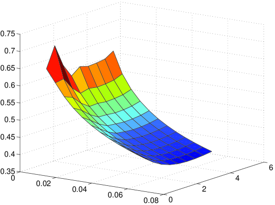
In order to showcase some prototypical volatility surfaces resulting from the proposed affine LIBOR models, we consider a tenor structure of zero coupon bond prices generated from the Svensson family. We fit the initial LIBOR rates implied by the bond prices using the $u$’s as described in Proposition 6.1, and then price caplets and plot the implied volatility surfaces for different parameters of the driving affine factor process. The implied volatility surface corresponding to the CIR parameters

$$\lambda=0.026,\quad\theta=0.65,\quad\eta=0.5\quad\text{and}\quad X_{0}=3.45$$

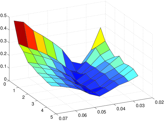
is shown in Figure 1. The implied volatilities from the CIR model exhibit a skewed shape as a function of strike price, while the term structure is decreasing as a function of maturity. In the example corresponding to the $\Gamma$-OU process, we consider the same tenor structure and the implied volatility surface corresponding to the $\Gamma$-OU parameters

$$\lambda=.05,\quad\alpha=0.8,\quad\beta=0.5,\quad X_{0}=1.35$$

is shown in Figure 2. The implied volatility exhibits a smile shape in this example, while we can still observe a decreasing behavior for the term structure of volatilities.

Figure 1. Implied volatility surface for the CIR martingales.

Figure 2. Implied volatility surface for the $\Gamma$-OU martingales.

Finally, let us point out that these figures stem from 1-factor models; one would expect to observe even flexible shapes of surfaces from multi-factor affine LIBOR models. Several impressive results in this direction have been obtained by DaFonseca_Gnoatto_Grasselli_2011 DaFonseca_Gnoatto_Grasselli_2011 .

References

- [\citeauthoryearAndersen and Brotherton-RatcliffeAndersen and Brotherton-Ratcliffe2005] Andersen, L. and R. Brotherton-Ratcliffe (2005). Extended LIBOR market models with stochastic volatility. J. Comput. Finance 9, 1–40.
- [\citeauthoryearBlackBlack1976] Black, F. (1976). The pricing of commodity contracts. J. Financ. Econ. 3, 167–179.
- [\citeauthoryearBrace, Ga̧tarek, and MusielaBrace et al.1997] Brace, A., D. Ga̧tarek, and M. Musiela (1997). The market model of interest rate dynamics. Math. Finance 7, 127–155.
- [\citeauthoryearBrigo and MercurioBrigo and Mercurio2006] Brigo, D. and F. Mercurio (2006). Interest Rate Models: Theory and Practice (2nd ed.). Springer.
- [\citeauthoryearCollin-Dufresne and GoldsteinCollin-Dufresne and Goldstein2002] Collin-Dufresne, P. and R. S. Goldstein (2002). Pricing swaptions within an affine framework. J. Derivatives 10, 9–26.
- [\citeauthoryearda Fonseca, Gnoatto, and Grassellida Fonseca et al.2011] da Fonseca, J., A. Gnoatto, and M. Grasselli (2011). A flexible matrix LIBOR model with smiles. Preprint.
- [\citeauthoryearDuchesne and de MicheauxDuchesne and de Micheaux2010] Duchesne, P. and P. L. de Micheaux (2010). Computing the distribution of quadratic forms: Further comparisons between the Liu–Tang–Zhang approximation and exact methods. Comput. Statist. Data Anal. 54, 858–862.
- [\citeauthoryearDuffie, Filipović, and SchachermayerDuffie et al.2003] Duffie, D., D. Filipović, and W. Schachermayer (2003). Affine processes and applications in finance. Ann. Appl. Probab. 13, 984–1053.
- [\citeauthoryearEberlein, Glau, and PapapantoleonEberlein et al.2010] Eberlein, E., K. Glau, and A. Papapantoleon (2010). Analysis of Fourier transform valuation formulas and applications. Appl. Math. Finance 17, 211–240.
- [\citeauthoryearEberlein and KlugeEberlein and Kluge2006] Eberlein, E. and W. Kluge (2006). Exact pricing formulae for caps and swaptions in a Lévy term structure model. J. Comput. Finance 9, 99–125.
- [\citeauthoryearEberlein and ÖzkanEberlein and Özkan2005] Eberlein, E. and F. Özkan (2005). The Lévy LIBOR model. Finance Stoch. 9, 327–348.
- [\citeauthoryearFilipovićFilipović2005] Filipović, D. (2005). Time-inhomogeneous affine processes. Stochastic Process. Appl. 115, 639–659.
- [\citeauthoryearFriesFries2007] Fries, C. (2007). Mathematical Finance: Theory, Modeling, Implementation. Wiley.
- [\citeauthoryearGatarek, Bachert, and MaksymiukGatarek et al.2006] Gatarek, D., P. Bachert, and R. Maksymiuk (2006). The LIBOR Market Model in Practice. Wiley.
- [\citeauthoryearGlasserman and KouGlasserman and Kou2003] Glasserman, P. and S. G. Kou (2003). The term structure of simple forward rates with jump risk. Math. Finance 13, 383–410.
- [\citeauthoryearHubalek and KallsenHubalek and Kallsen2005] Hubalek, F. and J. Kallsen (2005). Variance-optimal hedging and Markowitz-efficient portfolios for multivariate processes with stationary independent increments with and without constraints. Working paper, TU München.
- [\citeauthoryearHunt, Kennedy, and PelsserHunt et al.2000] Hunt, P., J. Kennedy, and A. Pelsser (2000). Markov-functional interest rate models. Finance Stoch. 4, 391–408.
- [\citeauthoryearHunt and KennedyHunt and Kennedy2004] Hunt, P. J. and J. E. Kennedy (2004). Financial Derivatives in Theory and Practice (2nd ed.). Wiley.
- [\citeauthoryearHurd and ZhouHurd and Zhou2010] Hurd, T. R. and Z. Zhou (2010). A Fourier transform method for spread option pricing. SIAM J. Financial Math. 1, 142–157.
- [\citeauthoryearJacod and ShiryaevJacod and Shiryaev2003] Jacod, J. and A. N. Shiryaev (2003). Limit Theorems for Stochastic Processes (2nd ed.). Springer.
- [\citeauthoryearJamshidianJamshidian1989] Jamshidian, F. (1989). An exact bond option formula. J. Finance 44, 205–209.
- [\citeauthoryearJamshidianJamshidian1997] Jamshidian, F. (1997). LIBOR and swap market models and measures. Finance Stoch. 1, 293–330.
- [\citeauthoryearJamshidianJamshidian1999] Jamshidian, F. (1999). LIBOR market model with semimartingales. Working Paper, NetAnalytic Ltd.
- [\citeauthoryearJoshi and StaceyJoshi and Stacey2008] Joshi, M. and A. Stacey (2008). New and robust drift approximations for the LIBOR market model. Quant. Finance 8, 427–434.
- [\citeauthoryearKallsen and ShiryaevKallsen and Shiryaev2002] Kallsen, J. and A. N. Shiryaev (2002). The cumulant process and Esscher’s change of measure. Finance Stoch. 6, 397–428.
- [\citeauthoryearKawazu and WatanabeKawazu and Watanabe1971] Kawazu, K. and S. Watanabe (1971). Branching processes with immigration and related limit theorems. Theor. Probab. Appl. 16, 36–54.
- [\citeauthoryearKeller-ResselKeller-Ressel2008] Keller-Ressel, M. (2008). Affine processes – theory and applications to finance. Ph. D. thesis, TU Vienna.
- [\citeauthoryearKeller-Ressel and SteinerKeller-Ressel and Steiner2008] Keller-Ressel, M. and T. Steiner (2008). Yield curve shapes and the asymptotic short rate distribution in affine one-factor models. Finance Stoch. 12, 149–172.
- [\citeauthoryearKlugeKluge2005] Kluge, W. (2005). Time-inhomogeneous Lévy processes in interest rate and credit risk models. Ph. D. thesis, Univ. Freiburg.
- [\citeauthoryearKluge and PapapantoleonKluge and Papapantoleon2009] Kluge, W. and A. Papapantoleon (2009). On the valuation of compositions in Lévy term structure models. Quant. Finance 9, 951–959.
- [\citeauthoryearMiltersen, Sandmann, and SondermannMiltersen et al.1997] Miltersen, K. R., K. Sandmann, and D. Sondermann (1997). Closed form solutions for term structure derivatives with log-normal interest rates. J. Finance 52, 409–430.
- [\citeauthoryearMusiela and RutkowskiMusiela and Rutkowski1997] Musiela, M. and M. Rutkowski (1997). Martingale Methods in Financial Modelling. Springer.
- [\citeauthoryearNicolato and VenardosNicolato and Venardos2003] Nicolato, E. and E. Venardos (2003). Option pricing in stochastic volatility models of the Ornstein–Uhlenbeck type. Math. Finance 13, 445–466.
- [\citeauthoryearPapapantoleon, Schoenmakers, and SkovmandPapapantoleon et al.2011] Papapantoleon, A., J. Schoenmakers, and D. Skovmand (2011). On efficient and accurate log-Lévy approximations for Lévy-driven LIBOR models. Preprint, TU Berlin.
- [\citeauthoryearPapapantoleon and SiopachaPapapantoleon and Siopacha2010] Papapantoleon, A. and M. Siopacha (2010). Strong Taylor approximation of SDEs and application to the Lévy LIBOR model. In M. Vanmaele et al. (Eds.), Proceedings of the Actuarial and Financial Mathematics Conference, pp. 47–62.
- [\citeauthoryearPressPress1966] Press, S. J. (1966). Linear combinations of non-central chi-square variates. Ann. Math. Statist. 37, 480–487.
- [\citeauthoryearRevuz and YorRevuz and Yor1999] Revuz, D. and M. Yor (1999). Continuous Martingales and Brownian Motion (3rd ed.). Springer.
- [\citeauthoryearSandmann, Sondermann, and MiltersenSandmann et al.1995] Sandmann, K., D. Sondermann, and K. R. Miltersen (1995). Closed form term structure derivatives in a Heath–Jarrow–Morton model with log-normal annually compounded interest rates. In Proceedings of the Seventh Annual European Futures Research Symposium Bonn, pp. 145–165. Chicago Board of Trade.
- [\citeauthoryearSatoSato1999] Sato, K. (1999). Lévy Processes and Infinitely Divisible Distributions. Cambridge University Press.
- [\citeauthoryearSchrager and PelsserSchrager and Pelsser2006] Schrager, D. F. and A. A. J. Pelsser (2006). Pricing swaptions and coupon bond options in affine term structure models. Math. Finance 16, 673–694.
- [\citeauthoryearSiopacha and TeichmannSiopacha and Teichmann2011] Siopacha, M. and J. Teichmann (2011). Weak and strong Taylor methods for numerical solutions of stochastic differential equations. Quant. Finance 11, 517–528.
- [\citeauthoryearWalterWalter1996] Walter, W. (1996). Ordinary Differential Equations. Springer.