Quantum vacuum effects from boundaries of designer potentials

Abstract

Vacuum energy in quantum field theory, being the sum of zero-point energies of all field modes, is formally infinite but yet, after regularization or renormalization, can give rise to finite observable effects. One way of understanding how these effects arise is to compute the vacuum energy in an idealized system such as a large cavity divided into disjoint regions by pistons. In this paper, this type of calculation is carried out for situations where the potential affecting a field is not the same in all regions of the cavity. It is shown that the observable parts of the vacuum energy in such potentials do not fall off to zero as the region where the potential is nontrivial becomes large. This unusual behavior might be interesting for tests involving quantum vacuum effects and for studies on the relation between vacuum energy in quantum field theory and geometry.

I Introduction

In quantum field theory (QFT), the energy associated with the vacuum is formally proportional to the sum of energies of all field modes. In most situations of interest, the summation is ultraviolet divergent. Nonetheless, because the energy spectra of fields depend on boundary conditions, it can be argued that the total vacuum energy does too; changing boundary conditions can shift vacuum energy by a finite amount and produce physical and observable effects. For example, the vacuum energy of the electromagnetic field between two parallel conducting plates depends on their separation and induces a macroscopic force, known as the Casimir force, that can be measured experimentally (see e.g. Bordag:2001qi ; Milton:2004ya ). Beside the parallel plate setup, vacuum energy has been discussed and computed in a wide range of other situations and is known to depend subtly on both geometry and topology Bordag:2001qi ; Milton:2004ya ; Ambjorn:1981xw .

Vacuum energy is of fundamental importance for several reasons. Since its effects can be measured experimentally, it offers direct verification of theoretic techniques for extracting finite physical quantities from formally divergent expressions in QFT. There currently seems to be an essentially sound understanding of these issues in the laboratory context. However, since the gravitational field in standard theory couples to the stress-energy of matter fields and not to differences in energy, the discrepancy between the formally divergent value of the vacuum energy in QFT and the flatness of the observed universe is sometimes quoted in the context of the cosmological constant problem. Vacuum energy also appears in discussions of tests for extra dimensions (see e.g. Milton:2004ya ).

For these and other reasons, vacuum energy has been studied in the literature from many points of view (see e.g. the reviews Milton:2004ya ; Bordag:2001qi ; Ambjorn:1981xw ; Actor:1999nb as well as recent works involving pistons Cavalcanti:2003tw ; Hertzberg:2005pr ; Edery:2006td ; Lim:2008yv ; Zhai:2008tf ; Geyer:2008wb ). In one approach, the summation over field mode energies is regularized using an explicit cutoff $\Lambda$. This is a useful approach because it reveals that the divergent contributions to the vacuum energy are proportional to the volume and the boundaries of the region containing the field Cavalcanti:2003tw . In some situations, these divergent contributions can be removed or neutralized in a controlled fashion Cavalcanti:2003tw . Having parametrized them using the scale $\Lambda$, however, tempts one to ask the question whether their structural form, i.e. their proportionality to volume and boundary, can be observable. Related issues have been raised previously in discussions related to the role of boundary conditions and materials in vacuum energy calculations Barton:2001wd ; Schaden:2006 ; Jaffe:2003ji . In this paper, such terms are shown to be observable when the field potential is space dependent.

The next section introduces the particular field theory studied in this paper. It is a scalar field theory with a potential that is quadratic in the field and that is assumed to depend on position. The potential is used to define a cuboidal cavity to which the field is confined, on whose boundary the field obeys Dirichlet conditions, and within which the field has a constant mass $m$. In this setup, the vacuum energy can be explicitly computed using the regularization technique with cutoff $\Lambda$. In two dimensions, the vacuum energy contains terms that are proportional to the area and perimeter of the cavity in addition to other terms that are either finite independently of the cutoff $\Lambda$ or vanish when the cutoff is large. This result is then used in the context of a potential defining two adjacent regions in a large cavity to show, following Cavalcanti:2003tw , that the force on a piston separating the two regions is independent of the terms in the vacuum energy proportional to the area and perimeter. This calculation sets the stage for Secs. III and IV, but also extends Cavalcanti:2003tw by including the field mass and other recent works on cavities with pistons Hertzberg:2005pr ; Edery:2006td ; Lim:2008yv ; Zhai:2008tf ; Geyer:2008wb by discussing the effect of a soft piston on the observable force.

In Sec. III, the potential of the scalar field is manipulated in order to make the force on a set of pistons in a large cavity depend on the area and perimeter of one region of the cavity. Two distinct scenarios are described, each associated with its own designer potential. These scenarios are highly idealized but are nonetheless significant because they demonstrate that the physical effects of vacuum energy do not necessarily need to become negligible as the regions in the cavity become large. In Sec. IV, these scenarios are extended to three dimensions and their possible observability is discussed. Section V summarizes the results and discusses the implications of the proposed scenarios on the understanding of vacuum energy, including its role in the gravitational context.

II Quantum vacuum energy

Consider a scalar field $\phi$ in flat $d+1$ dimensional spacetime with Lagrangian ($\hbar=c=1$)

$$L=\frac{1}{2}\int d^{d}x\left[(\partial_{\mu}\phi)(\partial^{\mu}\phi)-V(x)\,\phi^{2}\right].$$ (1)

The potential term is quadratic in $\phi$ and its coefficient $V(x)$, hereafter also called the potential, is assumed to depend on the position $x$. Field modes $\phi_{\bf{n}}$ and their energies $\epsilon_{\bf{n}}$ are found by solving the eigenvalue equation

$$\left(V(x)-\nabla^{2}\right)\phi_{\bf{n}}(x)=\epsilon_{\bf{n}}^{2}\phi_{\bf{n}}(x)$$ (2)

with the appropriate boundary conditions. The potentials considered in this paper are variations of

$$V_{0}(x)=\left\{\begin{array}[]{ll}m^{2}&\quad 0<x_{i}<a_{i}\\ \infty&\quad{\mbox{elsewhere. }}\end{array}\right.$$ (3)

This potential defines a hypercuboidal cavity with side lengths $a_{1},a_{2},\ldots,a_{d}$ (which can be all different). The field has mass $m$ inside the cavity; the infinite potential outside the cavity imposes Dirichlet conditions on its boundary and prevents the field from leaking out. For $V(x)=V_{0}(x)$, field modes $\phi_{\bf{n}}(x)$ are given by standing waves and their energies are given by

$$\epsilon_{{\bf n}}^{2}=m^{2}+\left(\frac{\pi\,n_{1}}{a_{1}}\right)^{2}+\cdots+\left(\frac{\pi\,n_{d}}{a_{d}}\right)^{2},$$ (4)

with $n_{i}=1,2,\ldots,\infty$. The vacuum energy, being the sum of all field mode energies, is

$$E(a_{1},\ldots,a_{d};m)=\frac{1}{2}\sum_{n_{1}=1}^{\infty}\cdots\sum_{n_{d}=1}^{\infty}\epsilon_{{\bf n}}.$$ (5)

Since this expression is ultraviolet (UV) divergent, it must be manipulated in order to extract physical information from it.

One way to proceed is through analytic regularization. This technique can be successfully applied in many situations and returns a finite answer (see e.g. Ambjorn:1981xw ). However, because the technique automatically subtracts all divergent contributions to the vacuum energy, it also eliminates the possibility of understanding them in detail.

A different technique that leaves one more manual control involves introducing an explicit cutoff scale $\Lambda$ and modifying (5) into

$$E_{\Lambda}(a_{1},\ldots,a_{d};m)=\frac{1}{2}\sum_{n_{1}=1}^{\infty}\cdots\sum_{n_{d}=1}^{\infty}\epsilon_{{\bf n}}\,D_{\Lambda}(\epsilon_{\bf{n}}),$$ (6)

where

$$D_{\Lambda}(\epsilon_{\bf{n}})=D_{\Lambda}\!\left(\frac{n_{1}}{a_{d}},\cdots,\frac{n_{d}}{a_{d}};m\right)$$ (7)

is an analytic cutoff function that behaves as $D_{\Lambda}(\epsilon_{\bf{n}})\sim 1$ for $\epsilon_{\bf{n}}<\Lambda$ and $D_{\Lambda}(\epsilon_{\bf{n}})\sim 0$ for $\epsilon_{\bf{n}}\gg\Lambda$. This formula reduces to (5) for $\Lambda\rightarrow\infty$ but gives a finite energy otherwise, parametrizing the divergences in (5) using the scale $\Lambda$.

In $d=2$, when the potential $V_{0}(x)$ defines a rectangular cavity with side lengths $a_{1}$ and $a_{2}$, (6) becomes

$$E_{\Lambda}(a_{1},a_{2};m)=\frac{1}{2}\sum_{n_{1}=1}^{\infty}\sum_{n_{2}=1}^{\infty}\left(m^{2}+\left(\frac{\pi\,n_{1}}{a_{1}}\right)^{2}+\left(\frac{\pi\,n_{2}}{a_{2}}\right)^{2}\right)^{1/2}\!\!D_{\Lambda}\!\left(\frac{n_{1}}{a_{1}},\frac{n_{2}}{a_{2}};m\right).$$ (8)

The summations can be performed by applying the Abel-Plana formula

$$\sum_{n=0}^{\infty}F(n)=\int_{0}^{\infty}\!F(t)\,dt\,+\,\frac{1}{2}F(0)+\,i\int_{0}^{\infty}\!\frac{dt}{e^{2\pi t}-1}\left(F(it)-F(-it)\right).$$ (9)

This calculation is an extension of the one for the massless case in Cavalcanti:2003tw and yields the result

$$E_{\Lambda}(a_{1},a_{2};m)=(a_{1}\,a_{2})\,\mu_{3}(\Lambda,m)+(a_{1}+a_{2})\,\mu_{2}(\Lambda,m)+R_{\Lambda}(a_{1},a_{2};m).$$ (10)

In the first two terms, the functions $\mu_{3}(\Lambda,m)$ and $\mu_{2}(\Lambda,m)$ are

$$\mu_{3}(\Lambda,m) =\frac{1}{2\pi^{2}}\int_{0}^{\infty}\!\!du_{1}\!\int_{0}^{\infty}\!\!du_{2}\left(m^{2}+u_{1}^{2}+u_{2}^{2}\right)^{1/2}D_{\Lambda}\left(u_{1},u_{2};m\right)$$ (11)

$$\mu_{2}(\Lambda,m) =-\frac{1}{4\pi}\int_{0}^{\infty}\!\!du\,(m^{2}+u^{2})^{1/2}D_{\Lambda}(u,0;m).$$ (12)

The last term in (10), $R_{\Lambda}(a_{1},a_{2};m)$, is a complicated function of its parameters Cavalcanti:2003tw ; Hertzberg:2005pr ; Lim:2008yv ; Edery:2006td ; Zhai:2008tf . In most discussions of vacuum energy, it is this term that is of most physical interest. For the present discussion, however, it is sufficient to state that it is finite independently of the cutoff function (its dependence on the cutoff is only $O(\Lambda^{-1})$) and that it can be simplified to

$$R_{\Lambda}(a_{1},a_{2};m)\sim w\,m,$$ (13)

with $w$ some constant of order unity, when $\Lambda$ is large and either $m=0$ and $a_{1}\sim a_{2}\gg 1$, or $m\neq 0$, $ma_{1}\gg 1$, and $ma_{2}\gg 1$. That is, $R_{\Lambda}(a_{1},a_{2};m)$ is independent of $a_{1}$ and $a_{2}$ in these regimes.

If this setup were taken as a model for two wires of length $a_{2}$ separated by distance $a_{1}$, a physical quantity computable from $E_{\Lambda}(a_{1},a_{2};m)$ would be the force $F$ on one of the wires as a function of the separation distance,

$$\begin{split}F&=-\frac{\partial E_{\Lambda}(a_{1},a_{2};m)}{\partial a_{1}}\\ &=-a_{2}\,\mu_{3}(\Lambda,m)-\mu_{2}(\Lambda,m)-\frac{\partial R_{\Lambda}(a_{1},a_{2};m)}{\partial a_{1}}.\end{split}$$ (14)

There are at least two reasons why this would be a problematic result.

First, this force contains contributions that grow with the cutoff $\Lambda$. If the cutoff were to be taken to infinity, the resulting force would diverge and would therefore require further manipulation. A possibility for eliminating the divergences would be to try to subtract from (10) the vacuum energy associated with a region of flat space having the same shape but without special boundary conditions imposed. This Minkowski vacuum energy, however, would be of the form of the area term in (10), so the subtraction would fail to eliminate the divergent term proportional to the perimeter; the subsequently computed force would still contain a term that diverges for large $\Lambda$. Even if the cutoff $\Lambda$ were assumed to be finite, perhaps related to the Planck scale, there would still be a problem because (14) would be nonzero even when $a_{1}\rightarrow\infty$. Such behavior in three dimensions would be in conflict with basic observations.

Second, assuming that $a_{1}$ can be varied freely is in violations of assumptions made in the calculations of $E_{\Lambda}$. More specifically, changing $a_{1}$ by a finite length implies shifting the background potential $V_{0}(x)$ by an infinite amount. The problem of preserving the total background energy could be avoided by considering joint changes in $a_{1}$ and $a_{2}$, which preserve the area $a_{1}\,a_{2}$. In this case, the formula (14) would be modified but the first issue above would remain.

II.1 Hard Piston

An elegant resolution to these problems was proposed in Cavalcanti:2003tw . Instead of the small cavity with side lengths $a_{1}$ and $a_{2}$, consider the setup shown in Fig. 1 where a large cavity with fixed side lengths $A_{1}$ and $a_{2}$ is divided by a vertical piston into two regions, labeled $I$ and $II$, with side lengths $a_{1}$ by $a_{2}$ and $A_{1}-a_{1}$ by $a_{2}$, respectively. The position of the piston is chosen so that $A_{1}\gg a_{1}$. The potential $V(x)$ associated with this system is

$$V_{1}(x)=\left\{\begin{array}[]{ll}m^{2}&\quad{\mbox{regions}}\;I,II\\ \infty&\quad{\mbox{elsewhere, }}\end{array}\right.$$ (15)

where the piston is considered to be part of the region where the potential is infinite. The piston is therefore “hard” and enforces strict Dirichlet conditions on its surface.

Figure 1: A large cavity separated by a moveable piston into two disjoint regions. The notation (x,y) labels Cartesian coordinates of the corners of the regions.

The UV regulated vacuum energy $E_{\Lambda}^{I+II}$ for this configuration is the combination of the vacuum energies for the two regions,

$$E_{\Lambda}^{I+II}=E_{\Lambda}(a_{1},a_{2};m)+E_{\Lambda}(A_{1}-a_{1},a_{2};m).$$ (16)

Substituting the general form (10) for each term on the right hand side yields

$$\begin{split}E_{\Lambda}^{I+II}&=(A_{1}\,a_{2})\,\mu_{3}(\Lambda,m)+(A_{1}+2a_{2})\,\mu_{2}(\Lambda,m)\\ &\qquad+R_{\Lambda}(a_{1},a_{2};m)+R_{\Lambda}(A_{1}-a_{1},a_{2};m).\end{split}$$ (17)

The result again contains terms that diverge when $\Lambda\rightarrow\infty$, but these terms are here independent of the position of the piston $a_{1}$. The force associated with moving the piston, $F=\partial E_{\Lambda}^{I+II}/\partial a_{1}$, thus depends only on the regular terms $R_{\Lambda}$. Since these terms become independent of $a_{1}$ when $A_{1}\gg a_{1}\rightarrow\infty$, the force is then also zero consistently with results obtained using analytical regularization techniques Cavalcanti:2003tw .

In this setup, moving the piston also does not change the overall level of the background potential. This setup thus resolves both issues discussed in association with the calculation leading to (14). It does not do this by eliminating UV divergences but rather by neutralizing them by summing contributions to the vacuum energy from fields in two neighboring regions. Since in laboratory situations there always exists an outside region (region $II$) to a cavity under investigation (region $I$), this resolution is satisfactory for all practical purposes.

II.2 Soft Piston

In the above discussion, the force on a piston arises from the terms $R_{\Lambda}$ in (17), which in principle, depend on the cutoff $\Lambda$. That these terms depend only weakly on $\Lambda$ implies that predictions based on (17) are equivalent, in the practical sense, for any sufficiently large, but not necessarily infinite, $\Lambda$. This observation suggests that the force computable from (17) is actually due to low-energy effects and is independent of how very high energy modes respond to the piston. To see this, consider again the cavity in Fig. 1 together with the potential

$$V_{1,\,M}(x)=\left\{\begin{array}[]{ll}m^{2}&\quad{\mbox{regions}}\;I,\,II\\ M^{2}&\quad{\mbox{piston}}\\ \infty&\quad{\mbox{elsewhere, }}\end{array}\right.$$ (18)

which differs from (15) in that it is noninfinite on the piston - the piston is “soft.” It is assumed that $M\gg m$.

In this situation, the set of field modes is more complicated than before and will not be derived in detail. Heuristically, however, modes with energy much smaller than $M$ should be expected to be confined by both the outer cavity walls and the piston into the disjoint regions $I$ and $II$. In other words, these modes obey Dirichlet conditions on the piston as well as the cavity walls. Modes with energy much greater than $M$ should still be expected to be confined by the outer cavity walls but should be oblivious to the presence and position of the piston. These modes do not obey special conditions on the piston. To a zeroth approximation, the total vacuum energy of this system may be written as a sum of contributions from these two parts of the spectrum,

$$E^{I+II}_{\Lambda,\,M}=\sum_{\epsilon_{\bf{n}}<M}\epsilon_{\bf{n}}^{I+II}+\sum_{\epsilon_{\bf{n}}>M}\epsilon_{\bf{n}}^{I+II}$$ (19)

where

$$\sum_{\epsilon_{\bf{n}}<M}\epsilon_{\bf{n}}^{I+II} \sim E_{M}(a_{1},a_{2};m)+E_{M}(A_{1}-a_{1},a_{2};m)$$

$$\sim(A_{1}\,a_{2})\,\mu_{3}(M,m)+(A_{1}+2a_{2})\,\mu_{2}(M,m)$$

$$\qquad+R_{M}(a_{1},a_{2};m)+R_{M}(A_{1}-a_{1},a_{2};m).$$ (20)

and

$$\sum_{\epsilon_{\bf{n}}>M}\epsilon_{\bf{n}}^{I+II} \sim E_{\Lambda}(A_{1},a_{2};m)-E_{M}(A_{1},a_{2};m)$$

$$\sim(A_{1},a_{2})\left(\mu_{3}(\Lambda,m)-\mu_{3}(M,m)\right)$$

$$\qquad+(A_{1}+a_{2})\left(\mu_{2}(\Lambda,m)-\mu_{2}(M,m)\right)$$

$$\qquad+R_{\Lambda}(A_{1},a_{2};m)-R_{M}(A_{1},a_{2};m)$$ (21)

The contribution of the low energy sector is given by an expression analogous to (17) but with the cutoff, now regarded as a physical one, set to $M$. The contribution of the high energy sector is obtained by first calculating the sum of all mode energies in the large cavity without piston (using a cutoff $\Lambda$) and then subtracting a low energy part. The total still contains some terms that diverge in the $\Lambda\rightarrow\infty$ limit as in the case of the hard pistons; in this sense, the soft piston does not eliminate the divergent nature of the vacuum energy.

Out of all the terms comprising (19), the only ones that depend on $a_{1}$ are the regular parts $R_{M}$ in (20). When $M$ is large, these parts depend only negligibly on this scale. Therefore, the force on the soft piston in this cavity system is equivalent to the one obtained in the case for the hard piston. In the present calculation, however, the important terms are explicitly seen to arise from low-energy modes.

The above argument is very rough. To make it more precise, one would need to compute the energy using the exact spectrum of the field in the cavity. In this way it should be possible to estimate the $M$-dependent corrections to the vacuum energy and the force on the piston. For large $M$, however, $M$-dependent corrections should be negligible and the above conclusion should be valid. In particular, there should not be important corrections to the area and perimeter terms of the vacuum energy. This is because if there were, their dependence on $a_{1}$ would cancel from contributions from regions $I$ and $II$. The effect of soft boundary conditions has also been discussed elsewhere in the literature, e.g. Jaffe:2003ji .

III Boundary Effects

The calculations in the previous section reveal that divergences in the vacuum energy are proportional to the area and perimeter of a cavity, and that they need not be subtracted away in order to produce reasonable results for the force on a piston. This suggests the following question: can these nonstandard terms in the vacuum energy ever have observable consequences?

Consider the cavity configuration shown in Fig. 2. The outer walls have side lengths $A_{1}$ and $A_{2}$. There are two pistons, one horizontal and one vertical as shown, which divide the cavity into four regions $I$, $II$, $III$, and $IV$. It is assumed that the two pistons can move and thereby change the size and shape of the regions. Region $I$ is shown shaded because it is assumed that the potential is different there compared to the other regions. Below are two calculations based on this cavity using different potentials.

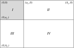
Figure 2: A large cavity separated into four regions by two moveable pistons.

III.1 Scenario 1

As a first example, consider Fig. 2 together with the potential

$$V_{2}(x)=\left\{\begin{array}[]{ll}m^{2}&\quad{\mbox{region}}\;I\\ 0&\quad{\mbox{regions}}\;II,III,IV\\ \infty&\quad{\mbox{elsewhere. }}\end{array}\right.$$ (22)

As before, the walls of the cavity and the pistons are taken to belong to the region where the potential is infinite, thus imposing Dirichlet boundary conditions there. This is a “designer” potential because the field is given different masses in different regions of space - a property not usually considered but perhaps not completely unreasonable in the context of theories implementing a dynamical mass-generation mechanism.

The vacuum energy for the total system is the sum of contributions from the individual regions. Denoting the entire cavity, regions $I+II+III+IV$ as $V$, the total vacuum energy becomes

$$\begin{split}E_{\Lambda}^{V}&=E_{\Lambda}(a_{1},a_{2};m)+E_{\Lambda}(A_{1}-a_{1},a_{2};0)\\ &\qquad+E_{\Lambda}(a_{1},A_{2}-a_{2};0)+E_{\Lambda}(A_{1}-a_{1},A_{2}-a_{2};0)\end{split}$$ (23)

Plugging in for each of the terms using (10) yields

$$\begin{split}E_{\Lambda}^{V}&\sim(A_{1}\,A_{2})\,\mu_{3}(\Lambda,0)+(a_{1}a_{2})\,\left[\mu_{3}(\Lambda,m)-\mu_{3}(\Lambda,0)\right]\\ &\qquad+2(A_{1}+A_{2})\,\mu_{2}(\Lambda,0)+(a_{1}+a_{2})\,\left[\mu_{2}(\Lambda,m)-\mu_{2}(\Lambda,0)\right]\end{split}$$ (24)

after ignoring all $R_{\Lambda}$ terms, which are negligibly small if the lengths involved are all large. In distinction with the calculation in the previous section, the vacuum energy now contains terms that depend on the area and perimeter of a single region, region $I$. The coefficients of these terms are nonzero.

Assuming

$$D_{\Lambda}(u,0;m)=D_{\Lambda}(u,0;0),$$ (25)

the coefficient of the perimeter term is

$$\mu_{2}(\Lambda,m)-\mu_{2}(\Lambda,0) =-\frac{1}{4\pi}\int_{0}^{\infty}du\;\left[(m^{2}+u^{2})^{1/2}-u\right]D_{\Lambda}(u,0;0)$$

$$<-\frac{1}{4\pi}\int_{U}^{\infty}du\left[(m^{2}+u^{2})^{1/2}-u\right]D_{\Lambda}(u,0;0)$$

$$<-O(m^{2}\log\Lambda/U)$$ (26)

The first line is an expansion of the $\mu_{2}$ functions using the definition (12). The integrand on this line is positive for all $u$ and thus justifies the inequality shown next. The scale $U>0$ on the second line can be chosen to be large so that the square root can be expanded in a series in $m$ around $m=0$. The leading term in the integrand becomes $m^{2}/2u$ and thus the integral depends logarithmically on the cutoff. A similar analysis for the other coefficient gives

$$\mu_{3}(\Lambda,m)-\mu_{3}(\Lambda,0)>O(m^{2}\Lambda).$$ (27)

As long as condition (25) holds, the scalings and signs in (26) and (27) are general and cannot be removed by choosing a special form for the cutoff function. If (25) does not hold, i.e. if the cutoff function is allowed to depend on $m$, then the mass $m$ can play a subtle role in the integrals and the dependence of the coefficients on the cutoff may in some cases be removed. However, even by tweaking the cutoff function in this manner, neither (26) or (27) can be made to vanish completely.

While both the area and perimeter terms are in principle observable, suppose that a constraint is imposed keeping the area $a_{1}a_{2}$ of region $I$ fixed. In this case the term proportional to the area would be unobservable. However, since the potential is fluid (by assumption), moving the pistons would change the vacuum energy by the term proportional to the perimeter, and this would produce a nonzero force. The sign of the perimeter term implies that the vacuum energy, given a fixed area $a_{1}a_{2}$, decreases as $a_{1}$ and $a_{2}$ become more unequal.

Suppose that the hard pistons were replaced by soft ones so that modes with energy larger than $M$ would need to satisfy Dirichlet conditions on the outer cavity walls but not on the piston. One aspect of this modification would be that the form (23) would be an accurate description of the contribution of only the low-energy modes. The coefficients of the area and perimeter terms would thus scale with $M$ rather than $\Lambda$. High energy modes should be relatively unaffected by the positions of the pistons and so might not produce important $\Lambda$-dependent terms either. The magnitude of the boundary contribution would thus not depend on the cutoff and the soft piston could be said to regularize the observable terms in the vacuum energy. It is important to note, however, that the source of the observable terms would not lie in the precise nature of the soft pistons but rather on the different masses of the scalar field in the various regions of the cavity. In any case, since soft boundary conditions can sometimes lead to subtle effects Jaffe:2003ji ; Schaden:2006 , this issue should be investigated in more detail. It is not unreasonable to suggest that a more realistic setup than the one described in this section might lead to vacuum energy terms that are independent of the cutoff $\Lambda$.

III.2 Scenario 2

As a second example, consider Fig. 2 and the potential

$$V_{3}(x)=\left\{\begin{array}[]{ll}m^{2}(\epsilon_{\bf{n}})&\quad{\mbox{region}}\;I\\ 0&\quad{\mbox{regions}}\;II,III,IV\\ \infty&\quad{\mbox{elsewhere. }}\end{array}\right.$$ (28)

Here, the mass of the field is not only different in the various regions of the cavity, but it is also dependent on the mode energy. The function $m(\epsilon_{\bf{n}})$ is assumed to be behave as $m(\epsilon_{\bf{n}})\sim 0$ for $\epsilon_{\bf{n}}\gg M$ and $m(\epsilon_{\bf{n}})\gg M$ for $\epsilon_{\bf{n}}<M$. Effectively, this makes region $I$ transparent to high energy modes but not to low energy ones.

The vacuum energy for this cavity, using again the notation $I+II+III+IV=V$, is

$$\begin{split}E_{\Lambda}^{V}&=\left[E_{\Lambda}(a_{1},a_{2};0)-G_{M}(a_{1},a_{2};0)\right]+E_{\Lambda}(A_{1}-a_{1},a_{2};0)\\ &\qquad+E_{\Lambda}(a_{1},A_{2}-a_{2};0)+E_{\Lambda}(A_{1}-a_{1},A_{2}-a_{2};0),\end{split}$$ (29)

where $G_{M}$ describes the effect of the potential on low-energy field modes in region $I$. Without this term, the sum of the remaining pieces produces a quantity in which all area and perimeter terms are independent of the piston positions $a_{1}$ and $a_{2}$. Any dependence of the vacuum energy on the piston positions is therefore encoded in the term $G_{M}$. If the mass function $m(\epsilon_{\bf{n}})$ is sufficiently sharp to eliminate all modes with energies up to the scale $M$,

$$m(\epsilon_{\bf{n}})=\left\{\begin{array}[]{ll}0&\quad{\mbox{if }}\;\epsilon_{\bf{n}}>M\\ \infty&\quad{\mbox{if }}\,\epsilon_{\bf{n}}\leq M,\end{array}\right.$$ (30)

then $G_{M}$ will have the same form as (10),

$$G_{M}(a_{1},a_{2};0)\sim(a_{1}\,a_{2})\,\mu_{3}(M,0)+(a_{1}+a_{2})\,\mu_{2}(M,0)+R_{M}(a_{1},a_{2};0).$$ (31)

If the area of region $I$ is constrained to be fixed, the first term is unobservable. The last term can be made negligibly small. That leaves only the boundary term. Interestingly, this term is now not divergent but is dependent on the scale $M$ associated with the nontrivial potential in region $I$. The result is a quantum vacuum effect that depends on the boundary of a region and a noninfinite energy scale. Since the sign of the boundary term is here opposite to that in the previous scenario, the vacuum energy is here lowest when $a_{1}\sim a_{2}$.

In this setup, since the observable terms in the vacuum energy are independent of $\Lambda$, replacing the hard pistons by soft ones would not change the core argument and result.

IV Three Dimensions

All the above arguments can be extended to three dimensions. The vacuum energy in a cuboidal cavity with side lengths $a_{1},$ $a_{2}$, and $a_{3}$ and potential $V_{0}$ in (3) is

$$\begin{split}E_{\Lambda}(a_{1},a_{2},a_{3};m)&=(a_{1}\,a_{2}\,a_{3})\,\mu_{4}(\Lambda,m)-\frac{1}{2}\,(a_{1}\,a_{2}+a_{1}\,a_{3}+a_{2}\,a_{3})\,\mu_{3}(\Lambda,m)\\ &\qquad-\frac{1}{2}\,(a_{1}+a_{2}+a_{3})\,\mu_{2}(\Lambda,m)+\!R_{\Lambda}(a_{1},a_{2},a_{3};m).\end{split}$$ (32)

Here $R_{\Lambda}(a_{1},a_{2},a_{3};m)$ is a regular function that, like $R_{\Lambda}(a_{1},a_{2};m)$ in two dimensions, becomes a constant in the limits $\Lambda\rightarrow\infty$ and $a_{1},a_{2},a_{3}\rightarrow\infty$ (see e.g. Ambjorn:1981xw ; Lim:2008yv ; Edery:2006td ). The functions $\mu_{3}(\Lambda,m)$ and $\mu_{2}(\Lambda,m)$ are the same as in (11) and (12), respectively, and $\mu_{4}(\Lambda,m)$ is

$$\mu_{4}(\Lambda,m)=\frac{1}{2\pi^{3}}\int_{0}^{\infty}\!\!du_{1}\int_{0}^{\infty}\!\!du_{2}\int_{0}^{\infty}\!\!du_{3}\left(m^{2}+u_{1}^{2}+u_{2}^{2}+u_{3}^{2}\right)^{1/2}D_{\Lambda}(u_{1},u_{2},u_{3}).$$ (33)

Thus, the divergent terms are here proportional to the volume $V=a_{1}\,a_{2}\,a_{3}$, surface area $S=a_{1}\,a_{2}+a_{1}\,a_{3}+a_{2}\,a_{3}$, and total edge length $L=a_{1}+a_{2}+a_{3}$ of the cavity.

The three-dimensional analog of Fig. 2 is a cavity setup with one special region and $2^{3}-1=7$ trivial regions, separated by three moveable pistons. Assuming again that the volume of the nontrivial region is constant, the volume contribution in total vacuum energy cannot change when the pistons move. But shifts in the vacuum energy can be achieved through changes of the surface area $S$ and total edge length $L$. In a system analogous to the one in Sec. III.1, changes in vacuum energy would take the form

$$\Delta E_{\Lambda}\sim-(\Delta S)\,O(\Lambda m^{2})+(\Delta L)\,O(m^{2}\log\Lambda/m).$$ (34)

A system like the one in Sec. III.2 would produce vacuum energy changes on the order of

$$\Delta E_{\Lambda}\sim(\Delta S)\,O(M^{3})-(\Delta L)\,O(M^{2}).$$ (35)

Contributions from the regular parts $R_{\Lambda}$ are omitted in both formulas.

Consider now the following estimates for the magnitudes of these changes in vacuum energy. Consider first (35) and assume that $M$ is associated with the atomic scale, $M\sim 10^{3}eV$. Changing the perimeter of the filled region by one square meter and the edge lengths by one meter would give $\Delta E\sim 10^{23}eV$ and $\Delta E\sim 10^{13}eV$, respectively. Consider next (34) with $\Lambda\sim 10^{28}eV$ and $m\sim 10^{6}eV$, so that the cutoff is identified with the Planck scale and $m$ with the masses of elementary particles. Changing the perimeter of the filled region by a square meter and the edge lengths by one meter would now give $\Delta E\sim 10^{54}eV$ and $\Delta E\sim 10^{20}eV$, respectively.

In both cases, the described changes in vacuum energy are roughly comparable to thermal effects (given by $kT$ times a suitable macroscopic number of degrees of freedom). They are therefore not automatically ruled out by observations and may in fact play interesting roles in the physics of the described situations. The difficulties for observing these effects directly, however, come in producing the required potentials and in adjusting the shapes of the nontrivial regions in a controlled fashion.

V Conclusion

In summary, this paper considers vacuum energy associated with a quantum scalar field confined to various cuboidal cavities. These simple geometries allow one to compute the vacuum energies explicitly and regularize their divergences using a cutoff $\Lambda$. In general, these divergences are proportional to the size (volume) and shape (boundary) of the cavities. In calculations extending Cavalcanti:2003tw , it is shown that if a cuboidal cavity is divided into distinct regions by pistons, the forces on the pistons are independent of the volume and boundary terms if the mass of the field is the same in all regions. The forces are also argued to be independent of whether the pistons are infinitely hard or soft. In Secs. III and Sec. IV, however, it is shown that boundary terms in the vacuum energy can lead to observable effects under certain circumstances. Two distinct scenarios are proposed.

In the first scenario, introduced in Sec. III.1, the field is assumed to be massive in one region of a cavity, and massless in other regions. The mass discrepancy leaves an observable term in the vacuum energy that is proportional to the boundary of the region where the field is massive. This term also depends non-negligibly on the cutoff $\Lambda$ - it diverges if the cutoff is taken to infinity. This could be seen as a pathology or an opportunity, depending on the point of view. In any case, it is unclear whether the cutoff dependence is an artifact of using a particular form of the cutoff function or assuming, unrealistically, that the pistons separating the two regions of space are infinitely hard. It is possible that using soft pistons in that calculation may yield an effect that depends on the mass $m$ of the field or on another finite, intermediate scale that reflects the hardness or softness of the pistons. This issue is related to discussions of boundary conditions in other vacuum energy systems Jaffe:2003ji ; Schaden:2006 .

In the second scenario, described in Sec. III.2, one region of a cavity has a negligible potential for field modes with energy above a threshold $M$ and an effectively infinite potential for field modes with energy below $M$. The observable part of the vacuum energy in this case again contains a term proportional to the volume and boundary of the special region. The mass scale associated with the effect in this case is $M$. Curiously, the sign of the boundary effect is opposite to that in the first scenario.

These effects are interesting for both theoretical and observational reasons. On the theoretical side, the scenarios described test understanding of regularization and renormalization methods in QFT. In particular, a naive computation of vacuum energy in the first scenario with hard pistons, Sec. III.1, using analytic regularization techniques would not predict a boundary effect. The described effect thus differentiates the cutoff and analytic regularization approaches and offers a way to determine which is the more correct way of understanding vacuum energy in QFT. (The boundary effect in the second scenario, Sec. III.2, could be argued to arise also within the analytic regularization scheme.)

It is also interesting to compare the arguments and results of the two scenarios with other work which has shown that binding energies of bodies composed of a granular material are proportional to their volumes and boundaries Barton:2001wd . While the scaling of those effects is qualitatively similar to those in the two scenarios in Sec. III, there are important differences between the two sets of calculations. One important difference is in the style of calculation. The calculations (with hard pistons) in Sec. III are exact and do not depend on any subtraction prescription. They therefore emphasize the source of the observable volume and boundary terms as due to the nontrivial potential. Another important difference between the two approaches is that in the first scenario in Sec. III.1, the observable effects arise due to mass differences in distinct regions of space which can arise due to dynamics of a single field and can therefore arise in vacuum without interactions with any granular materials.

These effects might also have interesting implications for issues in quantum gravity. The idea that the Planck scale might provide a real UV cutoff for quantum field theory appears in many forms in the literature (see e.g. Garay for general arguments and e.g. Physicalcutoff1 ; Physicalcutoff2 ; Physicalcutoff3 ; Physicalcutoff4 for a few recent approaches). The present discussion suggests that quantum gravity models should take into account $\Lambda$-dependent contributions to the vacuum energy proportional to the boundary as well as the volume of the observable universe. That is, they should not only account for why the volume contribution to the vacuum energy does not generate a large cosmological constant, but should also explain the role of the boundary terms (for possible consequences of the boundary terms on geometry, see KonopkaDICE .)

On the observational side, the boundary terms are interesting because their magnitudes increase with the size of a region. This is an interesting behavior for vacuum energy whose effects, apart in the case of materials Barton:2001wd , are usually inversely proportional to the separation between boundaries and therefore vanish for large systems. Also, in contrast with other works where boundaries have been found to play a role (e.g. Wagner:2008qq ), the effects described in this paper are dominant and not corrections. Simple estimates of the magnitudes of the boundary energies in three dimensions in Sec. IV show that they can be on the order of thermal energies and hence that they are not immediately ruled out by existing observations. Testing for the boundary energies should therefore be interesting as a matter of principle. In practice, however, observation might be difficult due to the peculiar potentials required and due to the necessity of changing the shape and volume of regions of space in a precise and controlled fashion.

- (1) M. Bordag, U. Mohideen and V. M. Mostepanenko, Phys. Rept. 353, 1 (2001) [arXiv:quant-ph/0106045].
- (2) K. A. Milton, J. Phys. A 37, R209 (2004). [arXiv:hep-th/0406024].
- (3) J. Ambjorn and S. Wolfram, Annals Phys. 147, 1 (1983).
- (4) A. Actor, I. Bender and J. Reingruber, Fortsch. Phys. 48, 303 (2000) [arXiv:quant-ph/9908058].
- (5) R. M. Cavalcanti, Phys. Rev. D 69, 065015 (2004) [arXiv:quant-ph/0310184].
- (6) M. P. Hertzberg, R. L. Jaffe, M. Kardar and A. Scardicchio, Phys. Rev. Lett. 95, 250402 (2005) [arXiv:quant-ph/0509071].
- (7) A. Edery, Phys. Rev. D 75, 105012 (2007) [arXiv:hep-th/0610173].
- (8) S. C. Lim and L. P. Teo, arXiv:0807.3613 [hep-th].
- (9) X. h. Zhai, Y. y. Zhang and X. z. Li, Mod. Phys. Lett. A 24, 393 (2009) [arXiv:0808.0062 [hep-th]].
- (10) B. Geyer, G. L. Klimchitskaya and V. M. Mostepanenko, Eur. Phys. J. C 57, 823 (2008) [arXiv:0808.3754 [quant-ph]].
- (11) G. Barton, J. Phys. A 34, 4083 (2001).
- (12) M. Schaden, Phys. Rev. A 73, 042102 (2006) [arXiv:hep-th/0509124].
- (13) R. L. Jaffe, AIP Conf. Proc. 687, 3 (2003) [arXiv:hep-th/0307014].
- (14) L. J. Garay, Int. J. Mod. Phys. A 10, 145 (1995) [arXiv:gr-qc/9403008].
- (15) S. Hossenfelder, Phys. Rev. D 73, 105013 (2006) [arXiv:hep-th/0603032].
- (16) A. Kempf, Phys. Rev. Lett. 92, 221301 (2004) [arXiv:gr-qc/0310035].
- (17) L. Smolin, Nucl. Phys. B 742, 142 (2006) [arXiv:hep-th/0501091].
- (18) L. Philpott, F. Dowker and R. Sorkin, arXiv:0810.5591 [gr-qc].
- (19) T. Konopka, arXiv:0903.4342 [gr-qc].
- (20) J. Wagner, K. A. Milton and P. Parashar, arXiv:0811.2442 [hep-th].