Quantum phase estimation with lossy interferometers

Abstract

We give a detailed discussion of optimal quantum states for optical two-mode interferometry in the presence of photon losses. We derive analytical formulae for the precision of phase estimation obtainable using quantum states of light with a definite photon number and prove that maximization of the precision is a convex optimization problem. The corresponding optimal precision, i.e. the lowest possible uncertainty, is shown to beat the standard quantum limit thus outperforming classical interferometry. Furthermore, we discuss more general inputs: states with indefinite photon number and states with photons distributed between distinguishable time bins. We prove that neither of these is helpful in improving phase estimation precision.

I Introduction

The strong sensitivity of certain quantum states to small variations of external parameters opens up great opportunities for devising high-precision measurements, e.g. of length and time, with unprecedented accuracy. A particularly important physical measurement technique is interferometry. Its numerous variations include Ramsey spectroscopy in atomic physics, optical interferometry in gravitational wave detectors, laser gyroscopes and optical imaging to name but a few. Understanding limits on its performance in realistic situations under given resources is therefore of fundamental importance to metrology. In this paper we examine the fundamental limits of the precision of optical interferometry in the presence of photon losses for quantum states of light with definite photon number.

Optical interferometry aims to estimate the relative phase of two modes, or two “arms”, of the interferometer. This estimation process requires a certain amount of resources which is typically identified to be the number of photons, $N$, used for the measurement. The best precision which can be obtained using classical states of light scales like $1/\sqrt{N}$, the so-called standard quantum limit (SQL). Using non-classical states of light this precision can be greatly improved, ideally leading to Heisenberg-limited scaling, $1/N$ Giovannetti et al. (2004, 2006). Indeed, recent years have seen many experimental proof-of-principle demonstrations of beating the SQL using quantum strategies in various interferometric setups  Mitchell et al. (2004); Eisenberg et al. (2005); Nagata et al. (2007); Resch et al. (2007); Higgins et al. (2007, 2008). Unfortunately, highly non-classical states of light which potentially lead to Heisenberg-limited sensitivity are very fragile with respect to unwanted but unavoidable noise in experiments. In quantum-enhanced optical interferometry, the loss of photons is the most common and potentially the most devastating type of noise that one encounters. In particular it was noted that highly entangled quantum states, optimal for interferometry in the lossless case – N00N states Bollinger et al. (1996) – are extremely fragile. Even for moderate losses they are outperformed by purely classical states Huelga et al. (1997); Shaji and Caves (2007); Sahovar and Milburn (2006); Rubin and Kaushik (2007); G. Gilbert and Weinstein (2008); Huver et al. (2008); Dorner et al. (2009). A different approach has been taken in Meiser and Holland (2008), where the noise arising from imperfect preparation of a state has been investigated.

In Dorner et al. (2009), the first systematic approach was taken in order to determine the structure of optical states optimal for interferometry in the presence of losses. The best possible precision using input states with definite photon number was given. In this paper we elaborate and extend the ideas presented in Dorner et al. (2009). Our treatment is based on general quantum measurement theory Helstrom (1976); Holevo (1982); Braunstein and Caves (1994); Braunstein et al. (1996). The quantity of interest is the lowest possible uncertainty attainable in parameter estimation, inversely proportional to the square root of the quantum Fisher information Braunstein and Caves (1994). The quantum Fisher information depends only on the state of the system and not on the measurement procedure. We show that the optimization of the quantum Fisher information can be done effectively over the class of input states which have a definite photon number. Since these input states are subject to unavoidable photon losses they will degrade into mixed states and their suitability for phase estimation is compromised. Our optimization takes this into account yielding the most suitable input states in the presence of photon losses leading to the highest possible quantum Fisher information, and hence to the best possible precision. We give a detailed description of the noise model and calculate an analytic expression for the quantum Fisher information. The latter is shown to be a concave function on a convex set and therefore suited for efficient convex optimization methods. We numerically determine the optimal input states, compare them to alternative quantum and classical strategies, and show that they can beat the SQL. We note that the corresponding precision, which lies between the SQL and the Heisenberg limit (depending on the loss rates), defines the best possible precision for optical two-mode interferometry. In addition to this we discuss a measurement procedure that allows one to achieve the optimal precision, in terms of a positive operator-valued measure (POVM), and the possibility of using states with indefinite photon number or distinguishable photons. We show that neither of these generalizations improves the estimation precision, and consequently the state with definite photon number and indistinguishable photons are optimal.

The paper is organized as follows. In Sec. II a general scheme of quantum phase estimation is presented, and the notion of optimality is defined. In Sec. III we introduce the quantum Fisher information and discuss its most important properties. In Sec. IV we derive an explicit formula for the quantum Fisher information and prove that it is a concave function of input state parameters. In Sec. V we discuss the structure of the optimal states for interferometry and compare them to alternative strategies and states. In Sec. VI we discuss a measurement with which it is possible to achieve optimal precision. Finally, in Sec. VII we discuss possible generalizations of the considered quantum states, particularly states with indefinite photon number and the case when photons are distinguishable.

II Phase estimation

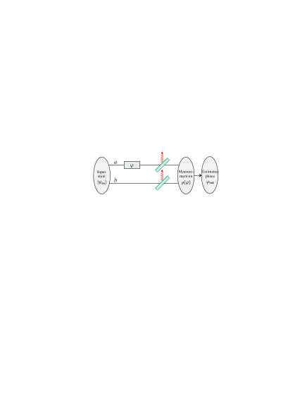
Figure 1: Interferometric phase estimation scheme. An input state is fed into an interferometer consisting of two channels. Channel $a$ acquires a phase $\varphi$ relative to channel $b$. Measurements are performed on the output state yielding an estimated value, $\varphi_{est}$, of the phase $\varphi$. The beam splitters symbolize photon losses.

We consider a general interferometer with two arms as shown in Fig. 1. A pure input state $|\psi_{in}\rangle$ is fed into the interferometer and acquires a phase $\varphi$ in the channel $a$ relative to the channel $b$. Both channels, or “arms”, of the interferometer are subject to photon losses which can be modelled by fictitious beam splitters inserted at arbitrary locations in both channels. The output of the interferometer therefore needs to be described in general by a mixed state $\rho(\varphi)$. A measurement, represented by a positive operator valued measure (POVM) $\{\Pi_{i}\}$ which defines a probability distribution for the measurement outcomes,

$$p(i|\varphi)=\textrm{Tr}\left[\Pi_{i}\rho(\varphi)\right],$$ (1)

is subsequently performed on the output state $\rho(\varphi)$. An estimated value of the true phase $\varphi$ is obtained by applying an estimator that assigns to a particular measurement result $i$ an estimated value $\varphi_{est}(i)$. We aim to estimate the phase $\varphi$ as precisely as possible.

Two more elements need to specified in order to make the problem of finding the optimal phase estimation strategy well defined: an a priori knowledge on the phase distribution $p(\varphi)$ and a cost function $C(\varphi,\varphi_{est})$ which can be seen as a measure for the uncertainty in the estimated phase. For phase estimation, the optimal choice of the input state, measurement and estimator is the one that minimizes the average cost function

$$\langle C\rangle=\int\textrm{d}\varphi\,p(\varphi)\sum_{i}p(i|\varphi)C(\varphi,\varphi_{est}(i)).$$ (2)

At this point two different approaches are most often pursued. In the global approach one assumes initial ignorance about the actual value of $\varphi$, which corresponds to the choice $p(\varphi)=1/2\pi$. The solution of the problem then yields an estimation strategy which performs equally well irrespectively of the actual value of the estimated phase. In the local approach, on the other hand, the assumption is that the value of the actual phase lies in the vicinity of a known phase $\varphi_{0}$. More precisely, the a priori probability is chosen to be $p(\varphi)=\delta(\varphi-\varphi_{0})$, while the estimator is required to be locally unbiased

$$\left.\frac{\textrm{d}}{\textrm{d}\varphi}\sum_{i}p(i|\varphi)\varphi_{est}(i)\right|_{\varphi=\varphi_{0}}=1.$$ (3)

The above condition is equivalent to a statement that the estimator will on average yield the true value of $\varphi$ up to the first order in $(\varphi-\varphi_{0})$. Notice that without local unbiasedness the estimation problem would be trivial (and also useless) since in order to minimize $\langle C\rangle$ in Eq. (2), with $p(\varphi)=\delta(\varphi-\varphi_{0})$, the optimal choice for the estimator would be simply $\varphi_{est}(i)=\varphi_{0}$, and the choice of the measurement would be irrelevant.

The local approach is useful when we are interested in small deviations of the phase from a known one. A significant advantage of the local approach over the global one is that for a natural choice of a quadratic cost function, there exist explicit lower bounds on $\langle C\rangle$ based on the Fisher information (see Sec. III). In many practical situations these bounds are tight and the optimization over the measurement and the estimator can be avoided. Moreover, the local approach may also be useful in situations when there is no a priori knowledge on the phase $\varphi$. If many copies of a state are given, one can first perform a rough measurement (even not optimal) on a small fraction of copies in order to narrow down the range of potential values of $\varphi$ so that they lie in a vicinity of a known phase $\varphi_{0}$, and then perform the optimal estimation using the local approach. This strategy will yield a high accuracy estimation for the global approach, without the need of optimizing the measurement and the estimator, since the rough measurement performed on small fraction of copies, even if not optimal, will not significantly influence the final accuracy Barndorff-Nielsen and Gill (2000).

III Fisher information

In what follows we take the local approach. Since in this case we deal with small deviations of estimated phases from the true one, it is natural to choose $C(\varphi,\varphi^{\prime})=(\varphi-\varphi^{\prime})^{2}$ as the cost function. Our goal is to find the optimal state, measurement and locally unbiased estimator minimizing the expression

$$(\delta\varphi)^{2}=\sum_{i}p(i|\varphi)[\varphi_{est}(i)-\varphi]^{2}.$$ (4)

To minimize the standard deviation $\delta\varphi$ given by the above formula we use an upper bound on $\delta\varphi$ based on the Fisher information Fisher (1925); Helstrom (1976). For a given POVM $\{\Pi_{i}\}$ and state $\rho(\varphi)$ defining the probabilities $p(i|\varphi)$, the Cramér-Rao inequality bounds the variance that can be obtained using any locally unbiased estimator,

$$(\delta\varphi)^{2}\geq\frac{1}{F},$$ (5)

where the Fisher information $F$ is given by

$$\quad F=\sum_{i}\frac{1}{p(i|\varphi)}\left(\frac{\partial p(i|\varphi)}{\partial\varphi}\right)^{2}.$$ (6)

If an experiment is repeated $\nu$ times the bound reads

$$(\delta\varphi)^{2}\geq\frac{1}{\nu F}.$$ (7)

For large $\nu$ the Cramér-Rao bound is asymptotically achieved by the maximum likelihood estimator Fisher (1925); Helstrom (1976); Braunstein and Caves (1994).

Optimization over the measurements yields the quantum Cramér-Rao bound Helstrom (1976); Holevo (1982); Braunstein and Caves (1994); Braunstein et al. (1996)

$$(\delta\varphi)^{2}\geq\frac{1}{F}\geq\frac{1}{F_{Q}},$$ (8)

where the quantum Fisher information $F_{Q}$ is given by

$$\quad F_{Q}=\textrm{Tr}[\rho(\varphi)A^{2}].$$ (9)

The Hermitian operator $A$ is called the “symmetric logarithmic derivative” (SLD) and is implicitly defined via the relation

$$\frac{\partial\rho(\varphi)}{\partial\varphi}=\frac{1}{2}[A\rho(\varphi)+\rho(\varphi)A].$$ (10)

In the eigenbasis of $\rho(\varphi)$, $A$ is given by

$$(A)_{ij}=\frac{2}{p_{i}+p_{j}}\left[\rho^{\prime}(\varphi)\right]_{ij},$$ (11)

where $\rho^{\prime}(\varphi)=\frac{\partial\rho(\varphi)}{\partial\varphi}$ and the $p_{i}$ are the eigenvalues of $\rho(\varphi)$ (whenever $p_{i}+p_{j}=0$ we set $(A)_{ij}=0$). It has been shown that a measurement saturating the quantum Cramér-Rao bound exists and is given by a projective measurement on the eigenbasis of $A$ Braunstein and Caves (1994); Braunstein et al. (1996).

For the sake of completeness we state some important properties of $F_{Q}$ (see e.g. Helstrom (1976); Fujiwara (2001)):

(i) Let $\rho(\varphi)$, $\sigma(\varphi)$ be two density matrices supported on orthogonal subspaces, $\mathcal{S}_{\rho(\varphi)}\bot\mathcal{S}_{\sigma(\varphi)}$, which do not cease to be orthogonal for an infinitesimal change of $\varphi$, i.e. $(\mathcal{S}_{\rho(\varphi)}\bigcup\mathcal{S}_{\rho^{\prime}(\varphi)})\bot(\mathcal{S}_{\sigma(\varphi)}\bigcup\mathcal{S}_{\sigma^{\prime}(\varphi)})$, then $F_{Q}$ is linear on the direct sum

$$F_{Q}[p\rho(\varphi)\oplus(1-p) \sigma(\varphi)]$$

$$=pF_{Q}[\rho(\varphi)]+(1-p)F_{Q}[\sigma(\varphi)].$$ (12)

(ii) $F_{Q}$ is convex

$$F_{Q}[p\rho(\varphi)+(1-p) \sigma(\varphi)]$$

$$\leq pF_{Q}[\rho(\varphi)]+(1-p)F_{Q}[\sigma(\varphi)]$$ (13)

(iii) For pure states $\rho(\varphi)=|\psi(\varphi)\rangle\langle\psi(\varphi)|$, $F_{Q}$ reads

$$F_{Q}=4[\langle\psi^{\prime}(\varphi)|\psi^{\prime}(\varphi)\rangle-|\langle\psi^{\prime}(\varphi)|\psi(\varphi)\rangle|^{2}],$$ (14)

where $|\psi^{\prime}(\varphi)\rangle=\partial|\psi(\varphi)\rangle/\partial\varphi$.

Property (i) is due to the fact that the SLD for $p\rho(\varphi)\oplus(1-p)\sigma(\varphi)$ is a direct product of SLDs for $p\rho(\varphi)$ and $(1-p)\sigma(\varphi)$, respectively. Property (ii) is a consequence of the fact that by (i) the right hand side of (ii) can be viewed as the quantum Fisher information of the state $p\rho(\varphi)\otimes|0\rangle\langle 0|+(1-p)\sigma(\varphi)\otimes|1\rangle\langle 1|$, where $|0\rangle$, $|1\rangle$ are orthogonal ancillary states, while the left hand side is $F_{Q}$ of the state after tracing out the ancillary system. Furthermore, $F_{Q}$ is non-increasing under stochastic operations Petz (1996) (tracing out the ancilla is an example). Property (iii) is a consequence of Eqs. (8,11), since for a pure state

$$A=2(|\psi(\varphi)\rangle\langle\psi^{\prime}(\varphi)|+|\psi^{\prime}(\varphi)\rangle\langle\psi(\varphi)|).$$ (15)

The measurement saturating the quantum Cramér-Rao bound in this case is a von Neumann measurement projecting on any orthonormal basis containing two vectors

$$|e_{\pm}\rangle=\frac{1}{\sqrt{2}}\left(|\psi(\varphi)\rangle\pm|\psi^{\prime\bot}(\varphi)\rangle\right),$$ (16)

where

$$|\psi^{\prime\bot}(\varphi)\rangle=\frac{1}{\mathcal{N}}(|\psi^{\prime}(\varphi)\rangle-\langle\psi(\varphi)|\psi^{\prime}(\varphi)\rangle|\psi(\varphi)\rangle)$$ (17)

is the normalized vector orthogonal to $|\psi(\varphi)\rangle$ lying in the space spanned by $|\psi(\varphi)\rangle$ and $|\psi^{\prime}(\varphi)\rangle$.

IV Interferometry with losses

Assuming that we have $N$ photons at our disposal, we aim to find the input state that allows performing phase estimation with the best precision possible, i.e. yielding the highest value of the quantum Fisher information $F_{Q}$. In particular we consider the most general pure two-mode input state with definite photon number $N$,

$$|\psi_{in}\rangle=\sum_{k=0}^{N}\alpha_{k}|k,N-k\rangle,$$ (18)

where $|k,N-k\rangle$ abbreviates the Fock state $|k\rangle_{a}|N-k\rangle_{b}$. This class of states includes the N00N state which, in the absence of losses, leads to Heisenberg limited precision, but is very fragile in the presence of noise. We are therefore looking for states which lead possibly to a lower precision than the N00N state, but which are more robust with respect to photon losses. Moreover, although states of the form (18) seem to be a restriction, we show in Sec. VII that our treatment effectively includes states with indefinite photon number.

In the following subsections we show how states of the form (18) are influenced by photon losses, calculate its quantum Fisher information and show that the latter can be maximized (thus minimizing $\delta\varphi$) by means of convex optimization methods.

IV.1 Noise model

Losses are modeled by fictitious beam splitters of transmissivity $\eta_{a}$, $\eta_{b}$ in channels $a$ and $b$ respectively, and cause a Fock state $|k,N-k\rangle$ to evolve into

$$|k,N-k\rangle\mapsto\sum_{l_{a}=0}^{k}\sum_{l_{b}=0}^{N-k}\sqrt{B_{l_{a}l_{b}}^{k}}|k-l_{a},N-k-l_{b}\rangle\otimes|l_{a},l_{b}\rangle,$$ (19)

where $|l_{a},l_{b}\rangle$ represents the state of two ancillary modes carrying $l_{a}$ and $l_{b}$ photons lost from modes $a$ and $b$ respectively, while

$$B^{k}_{l_{a}l_{b}}=\binom{k}{l_{a}}\binom{N-k}{l_{b}}\eta_{a}^{k}(\eta_{a}^{-1}-1)^{l_{a}}\eta_{b}^{N-k}(\eta_{b}^{-1}-1)^{l_{b}}.$$ (20)

Including the phase accumulation $|k,N-k\rangle\mapsto e^{ik\varphi}|k,N-k\rangle$ and tracing out the ancillary modes results in the output density matrix

$$\rho(\varphi)=\sum_{l_{a}=0}^{N}\sum_{l_{b}=0}^{N-l_{a}}p_{l_{a}l_{b}}|\xi_{l_{a}l_{b}}(\varphi)\rangle\langle\xi_{l_{a}l_{b}}(\varphi)|,$$ (21)

where

$$|\xi_{l_{a}l_{b}}(\varphi)\rangle=\frac{1}{\sqrt{p_{l_{a}l_{b}}}}\sum_{k=l_{a}}^{N-l_{b}}\alpha_{k}e^{ik\varphi}\sqrt{B_{l_{a}l_{b}}^{k}}|k-l_{a},N-k-l_{b}\rangle$$ (22)

is the conditional pure state corresponding to the event when $l_{a}$ and $l_{b}$ photons are lost in modes $a$ and $b$ respectively, and $p_{l_{a}l_{b}}$ is the normalization factor corresponding to the probability of that event.

Equivalently, the loss process can be described by a master equation for two independently damped harmonic oscillators with loss rates $\gamma_{a,b}=|\ln\eta_{a,b}|/t$, where $t$ is time, the solution of which is given by

$$\rho=\sum_{k,l=0}^{\infty}K_{l,a}K_{k,b}\rho_{in}K_{k,b}^{\dagger}K_{l,a}^{\dagger}$$ (23)

with Kraus operators

$$K_{l,a}=(1-\eta_{a})^{\frac{l}{2}}\eta_{a}^{\frac{1}{2}{\hat{a}}^{\dagger}\hat{a}}{\hat{a}}^{l}/\sqrt{l!},$$ (24)

where $\hat{a}$ is the annihilation operator for mode $a$, and analogously for mode $b$. This state acquires a phase through the transformation $\rho(\varphi)=\mathrm{e}^{-i\varphi\hat{a}^{\dagger}\hat{a}}\rho\mathrm{e}^{i\varphi\hat{a}^{\dagger}\hat{a}}$. Notice that thanks to the relation

$$\hat{a}^{l}e^{-i\varphi\hat{a}^{\dagger}\hat{a}}=e^{-i\varphi\hat{a}^{\dagger}\hat{a}}\hat{a}^{l}e^{i\varphi l}$$ (25)

we can commute the phase operator with the Kraus operators since the phase terms $e^{-i\varphi l}$ cancels out. It is therefore irrelevant if photons are lost before, during or after channel $a$ acquires its relative phase with respect to $b$.

IV.2 Calculating the Fisher information

Using Eq. (21) for the output state, one can calculate $F_{Q}$ with the help of Eqs. (8) and (11). This requires diagonalization of $\rho(\varphi)$ which can be carried out in the case of one-arm losses. In the more general case of losses in both arms an analytic calculation of $F_{Q}$ turns out to be infeasible. Nevertheless, we are able to determine an upper bound to the quantum Fisher information which, although not strictly tight for general input states, is very close to $F_{Q}$ for the states we consider in Sec. V.

IV.2.1 Losses in one arm

We consider first the case $\eta_{a}=\eta$, $\eta_{b}=1$, i.e. when losses are present in only one arm. As can be seen from Eq. (21), in this case only states $|\xi_{l_{a}l_{b}}(\varphi)\rangle$ with $l_{b}=0$ contribute to $\rho(\varphi)$. Moreover, we have $\langle\xi_{l0}(\varphi)|\xi_{l^{\prime}0}(\varphi)\rangle=\delta_{ll^{\prime}}$, hence we can write the output state as a direct sum

$$\rho(\varphi)=\bigoplus_{l=0}^{N}p_{l0}|\xi_{l0}(\varphi)\rangle\langle\xi_{l0}(\varphi)|.$$ (26)

Making use of Eqs. (III) and (14) we get a formula for $F_{Q}$ with explicit dependence on the input state parameters $\alpha_{k}$,

$$F_{Q}=4\left(\sum_{k=0}^{N}k^{2}x_{k}-\sum_{l=0}^{N}\frac{\left(\sum_{k=l}^{N}x_{k}kB^{k}_{l0}\right)^{2}}{\sum_{k=l}^{N}x_{k}B^{k}_{l0}}\right),$$ (27)

where $x_{k}=|\alpha_{k}|^{2}$. In a more compact way the above formula can be rewritten as

$$F_{Q}=2\sum_{l=0}^{N}\frac{\boldsymbol{x}^{T}\mathbf{R}^{(l0)}\boldsymbol{x}}{\boldsymbol{x}^{T}\boldsymbol{b}^{(l0)}},$$ (28)

where $\boldsymbol{x}$ is a vector containing variables $x_{k}$, while the elements of the vector $\boldsymbol{b}^{(l_{a}l_{b})}$ and the matrix $\mathbf{R}^{(l_{a}l_{b})}$ are given by

$$b^{(l_{a}l_{b})}_{k} =\left\{\begin{array}[]{ccl}B^{k}_{l_{a}l_{b}}&\textrm{ if }&l_{a}\leq k\leq N-l_{b}\\ 0&\textrm{otherwise}\end{array},\right.$$ (31)

$$R^{(l_{a}l_{b})}_{k,k^{\prime}} =b^{(l_{a}l_{b})}_{k}(k-k^{\prime})^{2}b^{(l_{a}l_{b})}_{k^{\prime}}.$$ (32)

IV.2.2 Losses in two arms

If losses are present in both arms, then, in the most general case, all $|\xi_{l_{a}l_{b}}(\varphi)\rangle$ contribute to $\rho(\varphi)$. States with different total number of lost photons, $l=l_{a}+l_{b}$, are still orthogonal. Using Eq. (III) we can therefore write

$$F_{Q}=\sum_{l=0}^{N}F_{Q}\left[\sum_{l_{a}=0}^{l}p_{l_{a}l-l_{a}}|\xi_{l_{a}l-l_{a}}(\varphi)\rangle\langle\xi_{l_{a}l-l_{a}}(\varphi)|\right],$$ (33)

where $F_{Q}[\cdot]$ denotes the quantum Fisher information of the state in brackets. Notice that states with the same $l$ are not necessarily orthogonal. Consequently, the calculation of the above expression requires solving an eigenvalue problem which is not feasible analytically. Nevertheless, using the convexity of $F_{Q}$, Eq. (III), we obtain a bound

$$F_{Q}\leq\tilde{F}_{Q}=\sum_{l_{a}=0}^{N}\sum_{l_{b}=0}^{N-l_{a}}p_{l_{a}l_{b}}F_{Q}[|\xi_{l_{a}l_{b}}(\varphi)\rangle\langle\xi_{l_{a}l_{b}}(\varphi)|],$$ (34)

which can be calculated explicitly using Eq. (14). It is given by

$$\tilde{F}_{Q}=4\left(\sum_{k=0}^{N}k^{2}x_{k}-\sum_{l=0}^{N}\sum_{m=0}^{N-l}\frac{\left(\sum_{k=l}^{N-m}x_{k}kB^{k}_{lm}\right)^{2}}{\sum_{k=l}^{N-m}x_{k}B^{k}_{lm}}\right),$$ (35)

or in a compact form,

$$\tilde{F}_{Q}=2\sum_{l_{a}=0}^{N}\sum_{l_{b}=0}^{N-l_{a}}\frac{\boldsymbol{x}^{T}\mathbf{R}^{(l_{a}l_{b})}\boldsymbol{x}}{\boldsymbol{x}^{T}\boldsymbol{b}^{(l_{a}l_{b})}}.$$ (36)

When losses are present only in one arm (see previous paragraph) $F_{Q}=\tilde{F}_{Q}$. When losses are present in both arms, however, the bound is not always tight. The difference $\tilde{F}_{Q}-F_{Q}$ originates from the non-orthogonality of $|\xi_{l_{a}l_{b}}(\varphi)\rangle$ for a fixed $l=l_{a}+l_{b}$, and physically corresponds to lack of knowledge about how many photons were lost from a particular mode. If this knowledge is not relevant then $\tilde{F}_{Q}=F_{Q}$. This happens, e.g. in the case of the N00N state $\alpha_{0}|N,0\rangle+\alpha_{N}|0,N\rangle$, when loss of even a single photon renders the output states useless for phase estimation, hence the knowledge of which mode the photons were lost does not influence the value of $F_{Q}$.

IV.3 Concavity of Fisher information

Even with the explicit formulae for $F_{Q}$ and $\tilde{F}_{Q}$ given by Eqs. (28) and (36) it is in general not possible to find an analytic solution for the optimal state, i.e. values $x_{k}\geq 0$, $\sum_{k}x_{k}=1$ that maximize $F_{Q}$ (or $\tilde{F}_{Q}$). However, we prove below that $\tilde{F}_{Q}$ is a concave function of the $\{x_{k}\}$. Consequently, the problem amounts to the maximization of a concave function $\tilde{F}_{Q}$ on a convex set. This allows for a feasible numerical constrained optimization using interior-point method routines (e.g. implemented in Mathematica 6.0), and more importantly, any local maximum found is automatically the global maximum.

We prove concavity by showing that the Hessian $H_{ij}=\frac{\partial^{2}\tilde{F}_{Q}}{\partial x_{i}\partial x_{j}}$ is negative semidefinite, i.e. for every vector $\boldsymbol{y}$ we have $\boldsymbol{y}^{T}\mathbf{H}\boldsymbol{y}\leq 0$. Using Eq. (36) the Hessian $H_{ij}$ ($i,j\in\{0,\dots,N\}$) reads

$$H_{ij}=4\sum_{k_{1}=0}^{N}\sum_{l_{b}=0}^{N-l_{a}}\frac{b^{(l_{a}l_{b})}_{i}b^{(l_{a}l_{b})}_{j}(\boldsymbol{x}^{T}\mathbf{R}^{(l_{a}l_{b})}\boldsymbol{x})-\boldsymbol{x}^{T}\boldsymbol{b}^{(l_{a}l_{b})}[b^{(l_{a}l_{b})}_{i}(\mathbf{R}^{(l_{a}l_{b})}\boldsymbol{x})_{j}+b^{(l_{a}l_{b})}_{j}(\mathbf{R}^{(l_{a}l_{b})}\boldsymbol{x})_{i}]+\boldsymbol{x}^{T}\boldsymbol{b}^{(l_{a}l_{b})}(\mathbf{R}^{(l_{a}l_{b})})_{i,j}\boldsymbol{x}^{T}\boldsymbol{b}^{(l_{a}l_{b})}}{(\boldsymbol{x}^{T}\boldsymbol{b}^{(l_{a}l_{b})})^{3}}.$$ (37)

Since the denominator is always positive, it is sufficient to prove that for every $l_{a}$, $l_{b}$ and for every vector $\boldsymbol{y}$ we have

$$(\boldsymbol{y}^{T}\boldsymbol{b}^{(l_{a}l_{b})})^{2}(\boldsymbol{x}^{T}\mathbf{R}^{(l_{a}l_{b})}\boldsymbol{x})-(\boldsymbol{x}^{T}\boldsymbol{b}^{(l_{a}l_{b})})(\boldsymbol{y}^{T}\boldsymbol{b}^{(l_{a}l_{b})})(\boldsymbol{y}^{T}\mathbf{R}^{(l_{a},l_{b})}\boldsymbol{x}+\boldsymbol{x}^{T}\mathbf{R}^{(l_{a},l_{b})}\boldsymbol{y})+(\boldsymbol{x}^{T}\boldsymbol{b}^{(l_{a}l_{b})})^{2}\boldsymbol{y}^{T}\mathbf{R}^{(l_{a}l_{b})}\boldsymbol{y}\leq 0.$$ (38)

Introducing $K_{ij}=(i-j)^{2}$, $w_{i}=y_{i}b^{(l_{a}l_{b})}_{i}(\boldsymbol{x}^{T}\boldsymbol{b}^{(l_{a}l_{b})})-x_{i}b^{(l_{a}l_{b})}_{i}(\boldsymbol{y}^{T}\boldsymbol{b}^{(l_{a}l_{b})})$ the above condition can be written equivalently as

$$\boldsymbol{w}^{T}\mathbf{K}\boldsymbol{w}\leq 0.$$ (39)

Since $\sum_{i}w_{i}=0$, it is sufficient to prove that $\mathbf{K}$ is negative semi-definite on the set of vectors with coefficients summing up to $0$. To this end we define vectors $\boldsymbol{e}^{(i)}$ ($i=1,\dots,N$), where $e_{0}^{(i)}=1$, $e^{(i)}_{i}=-1$, $e^{(i)}_{j}=0$ (for $j\neq 0$, $j\neq i$), which span the space of all vectors with coefficients summing up to zero. Writing $\boldsymbol{w}=\sum_{i=1}^{N}\beta_{i}\boldsymbol{e}^{(i)}$ and noticing that $\boldsymbol{e}^{(i)T}\mathbf{K}\boldsymbol{e}^{(j)}=-2ij$ we arrive at

$$\boldsymbol{w}^{T}\mathbf{K}\boldsymbol{w}=-2\sum_{i,j}\beta_{i}\beta_{j}ij=-2\left(\sum_{i}\beta_{i}i\right)^{2}\leq 0,$$ (40)

which proves that $\tilde{F}_{Q}$ is a concave function of the $\{x_{k}\}$.

V Optimal states for phase estimation

In this section we discuss optimization results based on Eqs. (27) and (35) derived in the previous sections. The quantity we analyze is $\delta\varphi_{min}\equiv 1/\sqrt{F_{Q}}$ corresponding to the best possible precision for a fixed number of measurements $\nu$ (cf. Eq. (8)). The only exception to this definition is in the case of the optimal state for losses in both arms where we set $\delta\varphi_{min}\equiv 1/\sqrt{\tilde{F}_{Q}}$ (see Sec. V.2). We compare the optimal precision to the precision which is obtainable using various alternative states and strategies. In particular, we define the standard interferometric limit (SIL) corresponding to the precision which can be achieved in a classical reference experiment. This serves as a benchmark by which we can judge the advantage of using quantum states of light over classical ones. For a given photon number $N$ the SIL is the precision of phase estimation using a Mach-Zehnder interferometer in which one arm gathers a phase $\varphi$, fed at one input port with a coherent state $|\alpha\rangle$, where $|\alpha|^{2}=N$, and the vacuum at the other port. The reflectivity of the two beam splitters can be adjusted to achieve the best precision, while the measurement consists of photon counting at the two output ports. Without any additional reference beams the input coherent state should be regarded as a state with unknown phase, and effectively described as a mixture of Fock states with Poissonian statistics (see Mølmer (1997), and the discussion in Sec. VII.1). By Eq. (III) the quantum Fisher information will be a weighted sum of quantum Fisher information calculated for each input Fock state after it passes through the first beam splitter. Taking the optimal value of transmissivity of the first beam splitter such that the ratio of the intensities in the arms $a$ and $b$ is $\sqrt{\eta_{b}/\eta_{a}}$ the final uncertainty in phase estimation achievable with this classical strategy is given by

$$\delta\varphi_{min,\textrm{SIL}}=\frac{\sqrt{\eta_{a}}+\sqrt{\eta_{b}}}{2\sqrt{N\eta_{a}\eta_{b}}}.$$ (41)

Note that the SIL scales in the same way as the SQL, particularly for equal losses in both arms we obtain $\delta\varphi_{\textrm{SIL}}=1/\sqrt{N\eta}$, where $\eta=\eta_{a}=\eta_{b}$.

As a reference let us also calculate the minimum uncertainty achievable using $N$ photons prepared in an unbalanced N00N state:

$$\sqrt{x_{N}}|N0\rangle+\sqrt{x_{0}}|0N\rangle.$$ (42)

The quantum Cramér-Rao bound yields:

$$\delta\varphi_{min,\textrm{N00N}}=\frac{\eta_{a}^{N/2}+\eta_{b}^{N/2}}{2N\eta_{a}^{N/2}\eta_{b}^{N/2}},$$ (43)

where the optimal amplitudes are given by

$$x_{0}=\frac{\eta_{a}^{N/2}}{\eta_{a}^{N/2}+\eta_{b}^{N/2}}$$ (44)

and $x_{N}=1-x_{0}$. Note that putting $N=1$ in Eq. (43) coincides with Eq. (41). This implies that a coherent state performs equally well in phase estimation as the equivalent number of single photons sent one-by-one. In the following we will concentrate on the two important scenarios of losses only in channel $a$ and equal losses in both channels.

V.1 Losses in one arm

The scenario of losses in only one arm of the interferometer, i.e. $\eta_{a}=\eta$ and $\eta_{b}=1$, is relevant, for example, if losses are induced by a sample itself. Figure 2 shows the parameters $x_{k}$ of the optimal state for $N=10$ photons as a function of $\eta$. The corresponding precision is shown in Fig. 3. The shaded, grey area in this figure is bounded by the SIL and the Heisenberg limit $1/N$, i.e. whenever a line is in this region there is an improvement over classical interferometry. The precision obtainable with the N00N state is worse than the SIL except for relatively low losses.

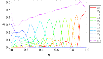
Figure 2: (color online). Parameters of the optimal state: $|\psi\rangle=\sum_{i=0}^{N}\sqrt{x_{i}}|i,N-i\rangle$, for phase estimation with $N=10$ photons for the case of losses in one only arm, i.e. $\eta_{a}=\eta$, $\eta_{b}=1$.

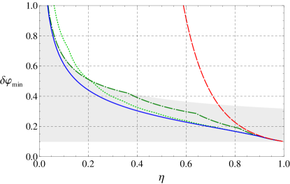
Figure 3: (color online). The minimal phase uncertainty achieved with various $N=10$ photon states for losses in one arm, i.e. $\eta_{a}=\eta$, $\eta_{b}=1$. Red, dashed line: N00N state; blue, solid line: optimal state (cf. Fig. 2); bright green, dotted line: optimal two-component state; dark green, dashed-dotted line: N00N chopping strategy. The shaded area is bounded by the SIL achievable with classical states and the Heisenberg limit $1/N$.

For transmissivities exceeding a certain threshold $\eta>\bar{\eta}$ the optimal state is equal to the N00N state (42). Note that for $\eta=1$ the N00N state is “balanced”, i.e. $x_{0}=x_{N}=1/2$. We will give an estimate for the threshold $\bar{\eta}$ at the end of this subsection. For $\eta<\bar{\eta}$ the optimal state consists of more components. As seen in Fig. 3 over a wide range we can achieve almost the same precision by using two-component states of the form

$$|\psi_{in}\rangle=\sqrt{x_{k}}|k,N-k\rangle+\sqrt{x_{N}}|N,0\rangle,$$ (45)

where we numerically optimize $k$ and the amplitude $x_{k}$. With decreasing $\eta$ the optimal choice for $k$ increases. This state is more robust in the presence of losses than a N00N state, since a loss of up to $k$ photons in the first mode does not destroy the superposition, while for the N00N state a loss of even a single photon renders the state useless for phase estimation. On the other hand, a large $N-k$ increases the sensitivity of the state with respect to an induced phase in channel $a$. The properties of large $k$ and large $N-k$ are therefore competing and the optimal result represents a trade-off between phase sensitivity and robustness.

An alternative strategy that leads to an improvement over the SIL, but uses states of a simpler structure than the optimal state is the N00N “chopping” strategy which was introduced in Ref. Dorner et al. (2009). Instead of a single N00N state, we use the same number of photons, but send them successively in $N/n$ smaller portions using $n$-photon n00n states. Repeating an experiment $N/n$ times corresponds to an $N/n$ fold increase in Fisher information, as shown in Eq. (7). Using Eq. (43) we find that the Fisher information for the N00N chopping strategy reads

$$F_{Q}=\frac{N}{n}\ \frac{4n^{2}\eta^{n}}{(1+\eta^{n/2})^{2}}.$$ (46)

Treating both $n$ and $N/n$ as real numbers with $n\in[1,N]$, maximization of this expression over $n$ yields

$$\delta\varphi_{min}=\begin{cases}\frac{1+\sqrt{\eta}}{2\sqrt{N\eta}}&;\eta\leq\eta_{0}\approx 0.228\\ \frac{1+\sqrt{\eta_{0}}}{2\sqrt{N\eta_{0}}}\sqrt{\frac{\ln{\eta}}{\ln{\eta_{0}}}}&;\eta_{0}<\eta\leq\eta_{0}^{\frac{1}{N}}\\ \frac{1+\eta^{\frac{N}{2}}}{2N\eta^{\frac{N}{2}}}&;\eta>\eta_{0}^{\frac{1}{N}}\end{cases}$$ (47)

where the optimal choice of $n$ for the three regimes indicated above is $n=1$, $n=1.478/|\ln{\eta}|$ (i.e. the solution of $1+\eta^{n/2}+n\ln\eta=0$) and $n=N$. We see that for very small transmissivities $\eta\leq\eta_{0}$ the precision is equal to the SIL, specified in Eq. (41). For higher transmissivities the chopping strategy beats the SIL, although only by a constant factor rather than in terms of scaling. For very high transmissivities $\eta>\eta_{0}^{1/N}$ the best strategy is to use un-chopped N00N states. We note that a similar strategy for multipartite qubit states has been devised in Shaji and Caves (2007).

As mentioned above the N00N state ceases to be optimal below a threshold $\bar{\eta}$ in which case the coefficient $x_{1}$ obtains a nonzero value. By adding an infinitesimal change $\delta x_{1}$ to $x_{1}$ at the expense of $x_{0},x_{N}$ (which we assume are kept in the proportion which is optimal in the absence of $x_{1}$), we can calculate the corresponding change in the quantum Fisher information. The change of $x_{1}$ by $\delta x_{1}$ increases $F_{Q}$ by $\frac{dF_{Q}}{dx_{1}}\delta x_{1}$, but at the same time due to decreasing weight of the other coefficients decreases it by $F_{Q}\delta x_{1}$. On the whole the change of $F_{Q}$ reads:

$$\delta F_{Q}=\left(\frac{dF_{Q}}{dx_{1}}-F_{Q}\right)\delta x_{1}.$$ (48)

Substituting $F_{Q}$ from Eq. (28) at $x_{0}=\eta^{N/2}/(1+\eta^{N/2})$, $x_{N}=1-x_{0}$, $x_{i}=0$ ($i=2,\dots,N-1$) and calculating $\delta F_{Q}$ we determine the value $\bar{\eta}$ below which $\delta F_{Q}/\delta x_{1}$ is positive. This implies that for $\eta<\bar{\eta}$ an increase in $x_{1}$ will increase $F_{Q}$. Writing $\delta F_{Q}/\delta x_{1}$ explicitly we get:

$$\frac{\delta F_{Q}}{\delta x_{1}}=\frac{4}{(1+\eta^{N/2})^{2}}[(1-2N)\eta^{N}-2N(N-1)\eta^{N/2+1}\\ +2(N-1)^{2}\eta^{N/2}-N(N-2)\eta+(N-1)^{2}].$$ (49)

The roots of the expression in square brackets can be found numerically. There is one real root in the interval $[0,1]$ which corresponds to the threshold $\bar{\eta}$. The roots behave in very good approximation like $\bar{\eta}=a^{-1/N}$ where $a\approx 2.61$ which is obtained by a fit to the roots between $N=5$ and $N=100$. For example, for $N=10$ we find that the threshold at which the N00N state ceases to be optimal is at $\bar{\eta}=0.91$, which agrees with the numerical results obtained before (see Fig. 2).

V.2 Equal losses in both arms

In order to determine the optimal state in the case of equal losses in both arms of the interferometer, i.e. $\eta_{a}=\eta_{b}\equiv\eta$, we use $\tilde{F}_{Q}$ as given by Eq. (35) as a basis for our numerical optimization. It simplifies maximization drastically since it is a concave function of the $\{x_{k}\}$. As pointed out in Sec. IV.2.2, $\tilde{F}_{Q}$, is only an upper bound to the “true” quantum Fisher information $F_{Q}$ and therefore cannot be reached by any measurement strategy if $F_{Q}$ is strictly smaller than $\tilde{F}_{Q}$. However, using $\tilde{F}_{Q}$ can be still very useful: We maximize $\tilde{F}_{Q}$ and use the resulting input state (say, $|\tilde{\psi}_{in}\rangle$) to calculate the corresponding $F_{Q}(|\tilde{\psi}_{in}\rangle)$. On the one hand, the true maximum of $F_{Q}(|\psi_{in}\rangle)$ (corresponding to the truly optimal state, $|\psi_{in}\rangle$) is certainly greater or equal to $F_{Q}(|\tilde{\psi}_{in}\rangle)$. On the other hand we have $F_{Q}(|\psi_{in}\rangle)\leq\tilde{F}_{Q}(|\psi_{in}\rangle)$ due to convexity [see Eq. (34)]. But since $\tilde{F}_{Q}(|\tilde{\psi}_{in}\rangle)$ is the global maximum we have $\tilde{F}_{Q}(|\psi_{in}\rangle)\leq\tilde{F}_{Q}(|\tilde{\psi}_{in}\rangle)$. Consequently, the true maximum must lie in between $F_{Q}(|\tilde{\psi}_{in}\rangle)$ and $\tilde{F}_{Q}(|\tilde{\psi}_{in}\rangle)$. Hence, if $|\tilde{F}_{Q}(|\tilde{\psi}_{in}\rangle)-F_{Q}(|\tilde{\psi}_{in}\rangle)|$ is small on a scale which is for this problem naturally given by the difference between the SIL and the Heisenberg limit, we obtain a very good approximation of the true maximal value of the quantum Fisher information. We showed numerically that for the examples discussed in this section this difference never exceeds $0.4\%$.

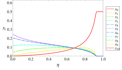
Figure 4: Parameters of the optimal state: $|\psi\rangle=\sum_{i=0}^{N}\sqrt{x_{i}}|i,N-i\rangle$, for phase estimation with $N=10$ photons for the case of equal losses in both arms, i.e. $\eta_{a}=\eta_{b}=\eta$. Due to this symmetry we have $x_{k}=x_{N-k}$.

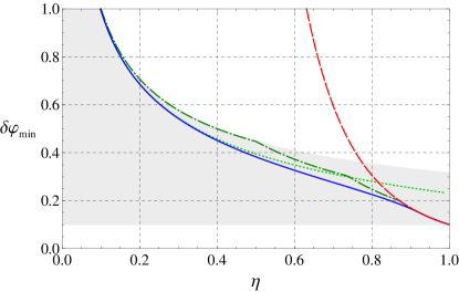
Figure 5: The minimal phase uncertainty achieved with various $N=10$ photon states for equal losses in both arms, i.e. $\eta_{a}=\eta_{b}=\eta$. Red, dashed line: N00N state; blue, solid line: optimal state (cf. Fig. 4); bright green, dotted line: the state optimal for lossless phase estimation in the global approach [see Eq. (50)]; dark green, dashed-dotted line: the N00N chopping strategy. The shaded area is bounded by the SIL achievable with classical states and the Heisenberg limit $1/N$.

The result of optimization is shown in Fig. 4 for $N=10$. Due to the symmetry of the problem, $\eta_{a}=\eta_{b}$, the solution has the property $x_{k}=x_{N-k}$. For small losses the optimal state is the balanced N00N state, i.e. $x_{0}=x_{N}=1/2$. However, below a threshold $\bar{\eta}$ all other terms $x_{k}$ obtain non-vanishing values. With decreasing $\eta$, $x_{0}$ and $x_{N}$ get smaller, and eventually the coefficients $x_{k}$ with $k\approx N/2$ are dominant. Interestingly, this structure is qualitatively similar to a two-mode generalization of the state which is optimal for one-mode lossless phase estimation in the global approach Berry and Wiseman (2000)

$$|\psi_{in}\rangle=\sqrt{2/(N+2)}\sum_{k=0}^{N}\sin[\pi(k+1)/(N+2)]|k,N-k\rangle.$$ (50)

It was noted in Ref. Maccone and De Cillis (2008) that these states perform quite well in the presence of loss, and hence could be useful for the problem we consider.

The threshold $\bar{\eta}$ can be obtained in a similar fashion as in the previous subsection. By adding an infinitesimal change $\delta x_{k}$ to a component $x_{k}$ other than $x_{0}$ and $x_{N}$ we can derive a polynomial which has a root in $[0,1]$ defining $\bar{\eta}(N)$. Since the polynomial is rather cumbersome we do not quote it here, however, the relevant root is again given in very good approximation by $\bar{\eta}=a^{-1/N}$ where $a\approx 2.24$ is obtained by a fit to the roots between $N=2$ and $N=100$. For example for $N=10$ (corresponding to Figs. 4 and 5) we get $\bar{\eta}=0.92$.

Analogous to the case of losses in only one arm we can examine a N00N chopping strategy by sending “smaller” n00n states through the interferometer. The corresponding precision reads

$$\delta\varphi_{min}=\begin{cases}\frac{1}{\sqrt{N\eta}}&;\eta\leq\mathrm{e}^{-1}\\ \sqrt{\frac{\mathrm{e}|\ln{\eta}|}{N}}&;\mathrm{e}^{-1}<\eta\leq\mathrm{e}^{-\frac{1}{N}}\\ \frac{1}{N\eta^{\frac{N}{2}}}&;\eta>\mathrm{e}^{-\frac{1}{N}}.\end{cases}$$ (51)

Figure 4 shows the estimation precision for the optimal state (blue line; here we use $\delta\varphi_{min}=1/\sqrt{\tilde{F}_{Q}}$), the N00N state (red line), the N00N chopping strategy (dark green line), and the state (50) (bright green line). In the latter case the precision is indeed quite high in the regime of high losses, outperforming the N00N chopping strategy but for small losses it is significantly worse than both the optimal and the N00N chopping strategies .

VI The optimal measurement

As discussed in Sec. III, a measurement saturating the quantum Cramér-Rao bound always exists. For the cases when the states $|\xi_{l_{a}l_{b}}(\varphi)\rangle$ introduced in Sec. IV are orthogonal for different $l=l_{a}+l_{b}$ (i.e. when $F_{Q}=\tilde{F}_{Q}$) we can derive an explicit POVM saturating the bound. To this end we first assume that we perform a measurement determining the total number of photons lost, $l$, which projects the system onto a particular pure state $|\xi_{l_{a}l_{b}}(\varphi)\rangle$ . Subsequently, we perform the measurement saturating the Cramér-Rao bound on pure states (see Sec. III), i.e. a projection on a basis containing the vectors

$$|e^{l_{a}l_{b}}_{\pm}\rangle=\frac{1}{\sqrt{2}}\left(|\xi_{l_{a}l_{b}}(\varphi)\rangle\pm|\xi^{\prime\bot}_{l_{a}l_{b}}(\varphi)\rangle\right)=\\ =\frac{1}{\sqrt{2}}\sum_{k=l_{a}}^{N-l_{b}}\alpha_{k}\sqrt{B^{k}_{l_{a}l_{b}}}\left(1\pm\frac{i(k-l_{a}-\langle\hat{n}_{a}\rangle_{l_{a}l_{b}})}{\sqrt{(\Delta\hat{n}_{a})^{2}_{l_{a}l_{b}}}}\right)e^{ik\varphi}|k-l_{a},N-k-l_{b}\rangle,$$ (52)

where $\langle\hat{n}_{a}\rangle_{l_{a}l_{b}}$, $(\Delta\hat{n}_{a})^{2}_{l_{a}l_{b}}$ are the mean photon number and the variance of the photon number in mode $a$ for the state $|\xi_{l_{a}l_{b}}(\varphi)\rangle$. The above POVM depends, in general, on the phase $\varphi$.

There are cases in which a single POVM saturating the Cramér-Rao bound for all values of $\varphi$ can be found. In a single photon case ($N=1$), states of the form $1/\sqrt{2}(|0,1\rangle+e^{i\chi}|1,0\rangle)$, allow for a $\varphi$-independent POVM, whereas states with unbalanced weights of $|01\rangle$, and $|10\rangle$ terms lead to optimal POVMs which are necessarily $\varphi$-dependent. Moreover, for an $N$ photon state $|\psi\rangle=\sum_{k=0}^{N}\alpha_{k}|k,N-k\rangle$, a single, $\varphi$-independent POVM saturating the Cramér-Rao bound can be found provided that the state enjoys the path-symmetry property: $\alpha_{k}=\alpha^{*}_{N-k}e^{i\chi}$, where $\chi$ is a fixed phase the same for all components Hofmann (2009). In general, due to losses the conditional pure states that appear in our problem lack the above mentioned symmetry and consequently the optimal POVM varies with the change of $\varphi$.

VII More general input states

One could argue that the $N$ photon state given by Eq. (18) does not represent the most general way of using $N$ photons to determine the relative phase in an interferometer: Instead of considering a state with a definite photon number $N$, one could consider a state which is a superposition of terms with different total photon number, and only imply a constraint that the mean photon number is $N$. Furthermore, by using states of the form (18) it is assumed that all photons in an arm of the interferometer are indistinguishable, i.e. occupy a common spatio-temporal mode. This greatly limits the class of considered states since the Hilbert space dimension of states sent into the interferometer would be of the order $2^{N}$ if the photons were distinguishable, while for indistinguishable photons it is $N+1$. In the next two subsections we show that none of these generalizations improves the phase estimation precision, and consequently it is sufficient to consider the states of the form given by Eq. (18).

VII.1 States with indefinite photon number

We emphasize that in this paper we consider closed systems, i.e. there are no additional reference beams, neither classical nor quantum, since any additional beam would contain photons and should therefore be explicitly taken into account for the determination of the required resources.

Consider a superposition of input states of the interferometer with different, but definite photon numbers $n$,

$$|\Psi_{in}\rangle=\sum_{n=0}^{\infty}\beta_{n}|\psi_{in}^{(n)}\rangle,$$ (53)

where the mean total photon number is $N=\sum_{n=0}^{\infty}|\beta_{n}|^{2}n$. Under free evolution a term with $n$ photons acquires a phase $e^{-in\omega t}$, i.e. terms with different $n$ evolve with different frequencies. In the absence of an additional reference beam which allows for clock synchronization between the sender and the receiver the relative phases between terms with different $n$ become unobservable and the state given by Eq. (53) is physically equivalent to a mixture Mølmer (1997); Bartlett et al. (2006),

$$\rho_{in}=\sum_{n=0}^{\infty}|\beta_{n}|^{2}|\psi^{(n)}_{in}\rangle\langle\psi^{(n)}_{in}|.$$ (54)

Moreover, since the quantum Fisher information is convex (see Sec. III), we have

$$F_{Q}(\rho_{in})\leq\sum_{n=0}^{\infty}|\beta_{n}|^{2}F_{Q}(|\psi^{(n)}_{in}\rangle\langle\psi^{(n)}_{in}|).$$ (55)

Consequently it is always better to send a state with a fixed number of photons $|\psi_{in}^{(n)}\rangle$, with probability $|\beta_{n}|^{2}$, rather than to use a superposition (which is effectively a mixture). The analysis can thus be restricted to states with definite photon number without compromising optimality.

VII.2 Distinguishability of photons

In this subsection we consider general $N$ photon input states where the photons are distinguishable which is the case, e.g., if they are sent in different time bins. A state of this type can be written as

$$|\psi_{in}\rangle=\sum_{\boldsymbol{k}=\boldsymbol{0}}^{\boldsymbol{1}}\alpha_{\boldsymbol{k}}|\boldsymbol{k}\rangle,$$ (56)

where $\boldsymbol{k}$ represents a binary sequence of length $N$, and $\boldsymbol{0}\equiv\{0,\dots,0\}$, $\boldsymbol{1}\equiv\{1,\dots,1\}$. Summation from a sequence to a sequence should be understood using partial ordering between sequences, i.e. $\boldsymbol{k}\leq\boldsymbol{k}^{\prime}\Leftrightarrow k_{i}\leq k^{\prime}_{i}\,\,\forall i$. Therefore the summation is performed over all binary sequences. Furthermore $|\boldsymbol{k}\rangle=|k_{1}\rangle\otimes\dots\otimes|k_{N}\rangle$ denotes a state of $N$ photons, where $k_{i}=0(1)$ means that the photon sent in the $i$-th time bin propagates in arm $a$ ($b$) of the interferometer. Mathematically, we deal here with an arbitrary $N$-qubit state, which lives in a $2^{N}$ dimensional space. Notice, that the indistinguishable case is recovered once we consider only the fully symmetric (bosonic) subspace of $N$ qubits.

$\tilde{F}_{Q}$ can be calculated in a similar way as in Sec. IV.2 and reads

$$\tilde{F}_{Q}=4\left(\sum_{\boldsymbol{k}=\boldsymbol{0}}^{\boldsymbol{1}}\bar{\boldsymbol{k}}^{2}x_{\boldsymbol{k}}-\sum_{\boldsymbol{l}_{a}=\boldsymbol{0}}^{\boldsymbol{1}}\sum_{\boldsymbol{l}_{b}=0}^{\boldsymbol{1}-\boldsymbol{l}_{a}}\frac{\left(\sum_{\boldsymbol{k}=\boldsymbol{l}_{a}}^{\boldsymbol{1}-\boldsymbol{l}_{b}}\bar{\boldsymbol{k}}x_{\boldsymbol{k}}B^{\boldsymbol{k}}_{\boldsymbol{l}_{a}\boldsymbol{l}_{b}}\right)^{2}}{\sum_{\boldsymbol{k}=\boldsymbol{l}_{a}}^{\boldsymbol{1}-\boldsymbol{l}_{b}}x_{\boldsymbol{k}}B^{\boldsymbol{k}}_{\boldsymbol{l}_{a}\boldsymbol{l}_{b}}}\right),$$ (57)

where boldface symbols denote binary strings of length $N$, $x_{\boldsymbol{k}}=|\alpha_{\boldsymbol{k}}|^{2}$, $\bar{\boldsymbol{k}}$ denotes the number of $1$s in the sequence $\boldsymbol{k}$, and

$$B^{\boldsymbol{k}}_{\boldsymbol{l_{a}}\boldsymbol{l_{b}}}=(1-\eta_{a})^{\bar{\boldsymbol{l}}_{a}}\eta_{a}^{\bar{\boldsymbol{k}}-\bar{\boldsymbol{l}}_{a}}(1-\eta_{b})^{\bar{\boldsymbol{l}}_{b}}\eta_{b}^{N-\bar{\boldsymbol{k}}-\bar{\boldsymbol{l}}_{b}}.$$ (58)

Again $\tilde{F}_{Q}=F_{Q}$ provided that knowledge from which mode a photon was lost is not relevant or self-evident, e.g. when $\eta_{b}=1$. Let us now symmetrize the state of $N$ photons. This corresponds to replacing $x_{\boldsymbol{k}}$ with $1/N!\sum_{\sigma}x_{\sigma(\boldsymbol{k})}$, where the summation is performed over all permutations of an $N$ element set. Notice that the first term within the parenthesis in Eq. (57) is not affected by symmetrization. Let us denote $a_{\boldsymbol{l}_{a}\boldsymbol{l}_{b}}=\sum_{\boldsymbol{k}=\boldsymbol{l}_{a}}^{\boldsymbol{1}-\boldsymbol{l}_{b}}\bar{\boldsymbol{k}}x_{\boldsymbol{k}}B^{\boldsymbol{k}}_{\boldsymbol{l}_{a}\boldsymbol{l}_{b}}$ and $b_{\boldsymbol{l}_{a}\boldsymbol{l}_{b}}=\sum_{\boldsymbol{k}=\boldsymbol{l}_{a}}^{\boldsymbol{1}-\boldsymbol{l}_{b}}x_{\boldsymbol{k}}B^{\boldsymbol{k}}_{\boldsymbol{l}_{a}\boldsymbol{l}_{b}}$. Then the subtracted term in Eq. (57) reads $\sum_{\boldsymbol{l}_{a}=\boldsymbol{0}}^{\boldsymbol{1}}\sum_{\boldsymbol{l}_{b}=0}^{\boldsymbol{1}-\boldsymbol{l}_{a}}\frac{a^{2}_{\boldsymbol{l}_{a}\boldsymbol{l}_{b}}}{b_{\boldsymbol{l}_{a}\boldsymbol{l}_{b}}}$. Performing symmetrization corresponds to replacing $a_{\boldsymbol{l}_{a}\boldsymbol{l}_{b}}$ and $b_{\boldsymbol{l}_{a}\boldsymbol{l}_{b}}$ with $1/N!\sum_{\sigma}a_{\sigma(\boldsymbol{l}_{a}),\sigma(\boldsymbol{l}_{b})}$ and $1/N!\sum_{\sigma}b_{\sigma(\boldsymbol{l}_{a}),\sigma(\boldsymbol{l}_{b})}$ respectively. Since $b_{\boldsymbol{l}_{a}\boldsymbol{l}_{b}}$ are positive, the following inequality holds

$$\frac{a_{\boldsymbol{l}_{a}\boldsymbol{l}_{b}}^{2}}{b_{\boldsymbol{l}_{a}\boldsymbol{l}_{b}}}+\frac{a_{\boldsymbol{l}^{\prime}_{a}\boldsymbol{l}^{\prime}_{b}}^{2}}{b_{\boldsymbol{l}^{\prime}_{a}\boldsymbol{l}^{\prime}_{b}}}\geq 2\frac{[1/2(a_{\boldsymbol{l}_{a}\boldsymbol{l}_{b}}+a_{\boldsymbol{l}^{\prime}_{a}\boldsymbol{l}^{\prime}_{b}})]^{2}}{1/2(b_{\boldsymbol{l}_{a}\boldsymbol{l}_{b}}+b_{\boldsymbol{l}^{\prime}_{a}\boldsymbol{l}^{\prime}_{b}})},$$ (59)

which shows that symmetrizing can only decrease the subtracted fraction, hence increase the Fisher information. This proves that the optimal states are symmetric states living in the bosonic subspace. Consequently, using indistinguishable photons is sufficient to obtain the optimal Fisher information.

A physical intuition behind the above derivation is the following. Notice that if there are no losses, the optimal $N$ qubit state has the form $1/\sqrt{2}(|\boldsymbol{0}\rangle+|\boldsymbol{1}\rangle)$ – it is the N00N state which lives in the fully symmetric subspace. In this case there is no advantage in using distinguishable photons. If there are losses, things get even worse for distinguishable photons. There is still no advantage in terms of phase sensitivity, yet when a photon is lost, the knowledge of which photon was lost additionally harms the quantum superposition. Hence, it is optimal to use states from a fully symmetric subspace, where it is not possible to tell which photon was actually lost.

VIII Summary

We have analyzed the optimal way of using $N$-photon states for phase interferometry in the presence of losses. We have derived an explicit formula for the quantum Fisher information in the case when losses are present in one arm of the interferometer, and have provided a useful bound for the case of losses in both arms. Using the quantum Fisher information as a figure of merit, we have found the optimal states, investigated their advantage over various quantum and classical strategies. The optimal measurement saturating the Cramér-Rao bound has been presented, and it has been proven that in general it varies depending on the phase in the vicinity of which we perform estimation.

A close inspection of the properties of the quantum Fisher information showed that it is optimal to use a quantum state with a definite number of indistinguishable photons. Neither allowing superpositions of different total photon-number terms, nor making photons distinguishable can improve estimation precision.