Sparse NonGaussian Component Analysis

Abstract

Non-gaussian component analysis (NGCA) introduced in [24] offered a method for high dimensional data analysis allowing for identifying a low-dimensional non-Gaussian component of the whole distribution in an iterative and structure adaptive way. An important step of the NGCA procedure is identification of the non-Gaussian subspace using Principle Component Analysis (PCA) method. This article proposes a new approach to NGCA called sparse NGCA which replaces the PCA-based procedure with a new the algorithm we refer to as convex projection.

keywords: reduction of dimensionality, model reduction, sparsity, variable selection, principle component analysis, structural adaptation, convex projection
Mathematical Subject Classification: 62G05, 60G10, 60G35, 62M10, 93E10

1 Introduction

Numerous mathematical applications in econometrics or biology are confronted with high dimensional data. Such data sets present new challenges in data analysis, since often the data have dimensionality ranging from hundreds to hundreds of thousands. This means an exponential increase of the computational burden for many methods. On the other hand the sparsity of the data in high dimensions entails that data thin out in the local neighborhood of a given point $\,x\,$. Hence statistical methods are not reliable in high dimensions if the sample size remains of the same order. This problem is usually referred to as ”curse of dimensionality” (cf. [8], [27]). The standard approach to deal with the high dimensional data is to introduce a structural assumption which allows to reduce the complexity or intrinsic dimension of the data without significant loss of statistical information [19], [17].

Let a random phenomenon is observed in the high dimensional space $\,\mathbb{R}^{d}\,$ while the intrinsic dimension of this phenomenon is much smaller, say $\,m\,$. From a geometrical point of view $\,m\,$ is the dimension of a linear subspace that approximately contains the structure of the sample data. Alternatively we can consider this structure as a low dimensional signal embedded in high dimensional noise. Consequently a lower dimensional, compact representation that according to some criterion, captures the interesting information in the original data, is sought. In this paper we assume that we have a sample of data lying approximately in a $\,m\leq d\,$ dimensional linear (target) subspace $\,\mathcal{I}\subseteq\mathbb{R}^{d}\,$ of $\,\mathbb{R}^{d}\,$. In order to reduce the problem dimension one looks for a mapping from the original data space onto this subspace.

In the statistical literature the Gaussian components of the data distribution are often considered as entropy maximizing and consequently as non-informative noise [5]. It is well known that for high-dimensional clouds of points most low-dimensional projections are approximately Gaussian [6]. The Non-Gaussian Component Analysis (NGCA), introduced in [24], is based on the assumption that the structure of the data is represented by a low dimensional non-Gaussian component of the observation distribution, as opposed to a full dimensional Gaussian component, considered as noise. Thus the objective of NGCA is to ”kill the noise” rather than to describe the whole multidimensional distribution. Note that the suggested way of treating the Gaussian distribution as a pure nuisance in general exclude the use of the classical Principle Component Analysis (PCA) which simply searches for the directions with of largest variance.

In the same way as a number of projection methods of feature extraction (e.g. Projection Pursuit [10], Partial Least Square Regression [28, 29], Conditional Minimum Average Variance Estimation [30] or Sliced Inverse Regression [15, 4, 2]), when implementing the NGCA we decompose the problem of dimension reduction into two tasks: the first one is to extract from data a set of vectors which are close to the target space $\,\mathcal{I}\,$; the second is to construct a basis of the target space from these vectors. These characteristics can also be found in the unsupervised, data driven approach of SNGCA, presented in this article. When compared to available dimension reduction methods (e.g. Principal Component Analysis [13], Independent Component Analysis [11] or Singular Spectrum Analysis [7]) SNGCA does not assume any a priori knowledge about the density of the original data.

The proposed method, as well as NGCA, is an iterative algorithm which is structure adaptive in the sense that every new step essentially uses the result of previous iterations. The main difference between NGCA and SNGCA algorithms lies in the way the information is extracted from the data. The algorithm of NGCA heavily relies upon the Euclidean projection and the PCA of the set of the estimated vectors. In the case when data dimension is important and the sample size is moderate, computation of the $\,l_{2}\,$-projection can amplify the noise. Moreover, when most of the estimated vectors do not contain information about the space $\,\mathcal{I}\,$ but are mainly noise, the results of using the PCA algorithm to extract the basis of feature space can be very poor. The reason for that is that the PCA algorithm is known to accumulate the noise. To address this issue the SNGCA uses convex programming techniques to estimate elements of the target subspace by “convex projection”, what allows to bound uniformly the estimation error. Further, another technique of convex analysis, based on computation of rounding ellipsoids of the set of estimated vectors, is used to extract the subspace information. These changes allow the SNGCA algorithm to treat large families of candidate vectors without increasing significantly the variance of the estimation of the target subspace.

The paper is organized as follows. First we describe the considered set-up in Section 2 and discuss the main ideas behind the proposed approach. The formal description of the algorithm is given in Section 3. A simulation study of the algorithms is presented in Section 4, where we compare the performance obtained by SNGCA algorithms and by several other methods of feature extraction.

2 Non-Gaussian Component Analysis

2.1 The setup

The following setting is due to [24]. Let $\,X_{1},...,X_{N}\,$ be i.i.d. from a distribution $\,I\!\!P\,$ in $\,\mathbb{R}^{d}\,$. We suppose that $\,I\!\!P\,$ possesses a density $\,\rho\,$ with respect to the Lebesgue measure on $\,\mathbb{R}^{d}\,$, which can be decomposed as follows:

$$\rho(x)=\phi_{\mu=0,\Sigma}(x)q(Tx).$$ (2.1)

Here $\,\phi_{\mu,\Sigma}\,$ stands for the density of the multivariate normal distribution $\,\mathcal{N}(\mu,\Sigma)\,$ with parameters $\,\mu\in\mathbb{R}^{d}\,$ (expectation) and $\,\Sigma\in\mathbb{R}^{d\times d}\,$ positive definite (covariance matrix). The function $\,q:\mathbb{R}^{m}\to\mathbb{R}\,$ with $\,m\leq d\,$ has to be nonlinear and smooth. $\,T\in\mathbb{R}^{m\times d}\,$ is an unknown linear mapping. Naturally, we refer to $\,\mathcal{I}={\rm range}\;T\,$ as target or non-Gaussian subspace. For the sake of simplicity let us assume $\,I\!\!E[X]=0\,$ where $\,I\!\!E[X]\,$ stands for the expectation of $\,X\,$.

Though the representation  (2.1) is not uniquely defined, the subspace $\,\mathcal{I}\subset\mathbb{R}^{d}\,$ is well defined as well as the Euclidean projector $\,\Pi^{*}\,$ on $\,\mathcal{I}\,$. By analogy with the regression case [4, 16, 15], we could also call $\,\mathcal{I}\,$ the effective dimension reduction space (EDR-space). We call $\,m\,$ effective dimension of the data. In many applications $\,m\,$ is unknown and has to be recovered from the data. Our task is to recover $\,\Pi^{*}\,$. The model structure  (2.1) allows the following interpretation (cf. [24]) : we can decompose the random vector $\,X\,$ into two independent components

$$X=\Pi^{*}X+(I-\Pi^{*})X=Z+u,$$

where $\,Z\,$ is a non-Gaussian $\,m\,$-dimensional signal and $\,u\,$ is $\,(d-m)\,$-dimensional normal noise.

As we have already noticed in the introduction, SNGCA algorithm relies upon two basic operations: the first is to construct a set of vectors, say $\,\beta_{1},...,\beta_{J}\,$, which are ”close” to the target subspace; the objective of the second is to compute an estimate $\,\widehat{\Pi}\,$ of the Euclidean projector $\,\Pi^{*}\,$ on $\,\mathcal{I}\,$ using the set $\,\{\beta_{j}\}_{j=1}^{J}\,$.

2.2 Estimation of elements of the target subspace

Estimation of elements of $\,\mathcal{I}\,$. The implementation of the first step of SNGCA is based on the following result (cf. Theorem 1 of [24]):

Theorem 1.

Let $\,X\,$ follow the distribution with the density $\,\rho\,$ which satisfies  (2.1) and let $\,I\!\!E[X]=0\,$. Suppose that a function $\,\psi:\,\mathbb{R}^{d}\to\mathbb{R}\,$ is continuously differentiable. Define

$$\beta(\psi):=I\!\!E\bigl{[}\nabla\psi(X)\bigr{]}=\int\nabla\psi(x)\,\rho(x)\,dx,$$ (2.2)

where $\,\nabla\psi\,$ stands for the gradient of $\,\psi\,$. Then there exists a vector $\,\beta\in\mathcal{I}\,$ such that

$$\|\beta(\psi)-\beta\|_{2} \leq \big{\|}\Sigma^{-1}I\!\!E[X\psi(X)]\big{\|}_{2}$$

$$= \Big{\|}\Sigma^{-1}\int x\psi(x)\rho(x)\;dx\Big{\|}_{2}.$$

In particular, if $\,I\!\!E[X\psi(X)]=0\,$, then $\,\beta(\psi)\in\mathcal{I}\,$.

The bound of Theorem 1 implies that

$$\|(I-\Pi^{*})\beta(\psi)\|_{2}\leq\Big{\|}\Sigma^{-1}\int x\psi(x)\rho(x)\;dx\Big{\|}_{2},$$ (2.3)

where $\,I\,$ is the $\,d\,$-dimensional identity matrix and $\,\Pi^{*}\,$ is the orthogonal projector on $\,\mathcal{I}\,$.

Based on this result, [24] suggested the following way of constructing a set of vectors $\,\beta\,$ which approximate the target space $\,\mathcal{I}\,$. Let $\,h_{1},...,h_{L}\,$ be smooth bounded functions on $\,\mathbb{R}^{d}\,$. Define $\,\gamma_{l}=I\!\!E[Xh_{l}(X)]\,$ and $\,\eta_{l}=I\!\!E[\nabla h_{l}(X)]\,$. These vectors are not computable because they rely on the unknown data distribution, but they can be well estimated from the given data. Next, for any vector $\,c\in\mathbb{R}^{L}\,$, define the vectors $\,\beta(c),\gamma(c)\in\mathbb{R}^{d}\,$ with

$$\beta(c)=\sum_{l=1}^{L}c_{l}\eta_{l},\qquad\gamma(c)=\sum_{l=1}^{L}c_{l}\gamma_{l}$$

Then by Theorem 1, $\,\beta(c)\in\mathcal{I}\,$ conditioned that $\,\gamma(c)=0\,$. Indeed, if we set $\,\psi(x)=\sum_{l}c_{l}h_{l}(x)\,$, then $\,I\!\!E[X\psi(X)]=0\,$, and by  (2.3),

$$\gamma(c)=I\!\!E[\nabla\psi(X)]\in\mathcal{I}.$$

The approach of [24] is to compute the vectors of coefficients $\,c\in\mathbb{R}^{L}\,$ which ensure $\,\gamma(c)\approx 0\,$ and then to use the corresponding empirical analogs of $\,\beta(c)\,$ to estimate the target space. More precisely, given the observations $\,X_{1},...,X_{N}\,$ compute the set of vectors (empirical counterparts of $\,\eta_{l}\,$ and $\,\gamma_{l}\,$) according to

$$\widehat{\gamma}_{l}=N^{-1}\sum_{i=1}^{N}X_{i}h_{l}(X_{i}),\quad\widehat{\eta}_{l}=N^{-1}\sum_{i=1}^{N}\nabla h_{l}(X_{i}).\qquad$$ (2.4)

Similarly define for $\,c\in\mathbb{R}^{L}\,$

$$\widehat{\beta}(c)=\sum_{l=1}^{L}c_{l}\widehat{\eta}_{l},\qquad\widehat{\gamma}(c)=\sum_{l=1}^{L}c_{l}\widehat{\gamma}_{l}\,.$$

One can expect that for vectors $\,c\,$ with $\,\widehat{\gamma}(c)=0\,$, the vectors $\,\widehat{\beta}(c)\,$ are ”close” to $\,\mathcal{I}\,$.

Below we follow a similar way of constructing $\,\widehat{\beta}(c)\,$ with an additional constraint that the considered vectors of coefficients $\,c\,$ satisfy $\,\|c\|_{1}\leq 1\,$. This constraint allows for both efficient numerical algorithms and sharp error bounds.

The test functions $\,h_{l}\,$ can be generated as follows: let $\,\mathcal{B}_{d}\,$ be a unit ball $\,\mathcal{B}_{d}=\{x\in\mathbb{R}^{d}|:\,\|x\|_{2}\leq 1\}\,$ and let $\,f(x,\omega)\,$, $\,f:\,\mathcal{B}\times\mathbb{R}^{d}\to\mathbb{R}\,$ be a continuously differentiable function. Consider the functions $\,h_{l}(x)=f(x,\omega_{l})\,$, for some $\,\omega_{l}\in\mathcal{B},\;l=1,...,L\,$. The choice of family $\,f(\cdot,\omega)\,$ is an important parameter of the algorithm design. For instance, in the simulation examples of Section 4 we consider the following families:

$$f(x,\omega) = \tanh(\omega^{\top}x)e^{-\alpha\|x\|^{2}_{2}/2},$$ (2.5)

$$f(x,\omega) = [1+(\omega^{\top}x)^{2}]^{-1}\exp^{\omega^{\top}x-\alpha\|x\|^{2}_{2}/2},$$ (2.6)

and $\,\omega_{l},\;l=1,...,L\,$ are unit vectors in $\,\mathbb{R}^{d}\,$. The next result justifies the proposed construction.

Theorem 2.

Suppose that $\,f\,$ is continuously differentiable in $\,w\,$ and for some fixed constant $\,f^{*}_{1}\,$ and any $\,\omega\in\mathcal{B}_{d},\,x\in\mathbb{R}^{d}\,$

$$\operatorname{Var}\bigl{[}X_{j}\,f(X,\omega)\bigr{]}\leq f^{*}_{1},\quad\operatorname{Cov}\bigl{[}X_{j}\,\nabla_{\omega}f(X,\omega)\bigr{]}\leq f^{*}_{1}I,$$

$$\operatorname{Var}\biggl{[}\frac{\partial}{\partial x_{j}}f(X,\omega)\biggr{]}\leq f^{*}_{1},\quad\operatorname{Cov}\biggl{[}\nabla_{\omega}\frac{\partial}{\partial x_{j}}f(X,\omega)\biggr{]}\leq f^{*}_{1}I,$$

Consider the (random) set

$$\mathscr{C}=\bigl{\{}c\in\mathbb{R}^{L}:\|c\|_{1}\leq 1,\,\widehat{\gamma}(c)=0\bigr{\}}.$$ (2.7)

Then for any $\,\varepsilon>0\,$ there is a set $\,A\subset\Omega\,$ of probability at least $\,1-\varepsilon\,$ such that on $\,A\,$ for all $\,c\in\mathscr{C}\,$,

$$\bigl{\|}(I-\Pi^{*})\widehat{\beta}(c)\bigr{\|}_{2}\leq\sqrt{d}\,\delta_{N}\bigl{(}1+\|\Sigma^{-1}\|_{2}\bigr{)},$$

where

$$\delta_{N}=N^{-1/2}\inf_{\lambda\leq\lambda^{*}_{1}N^{1/2}}\bigl{\{}5\mathfrak{n}_{0}f^{*}_{1}\lambda+2\lambda^{-1}\bigl{[}\mathfrak{e}_{d}+\log(2d/\varepsilon)\bigr{]}\bigr{\}}$$

and $\,\mathfrak{e}_{d}=4d\log 2\,$.

The proof of the theorem is given in the appendix.

Due to this result, any vector $\,c\in\mathscr{C}\,$ can be used to produce a vector $\,\widehat{\beta}(c)\,$ which is close to the target subspace $\,\mathcal{I}\,$. However, such constructed vectors are only informative if its length is significant relative to the estimation error.

We therefore compute a family of such coefficient vectors $\,c\,$ by solving the following optimization problems: for a fixed unit vector $\,\xi\in\mathbb{R}^{d}\,$ called a probe vector, find

$$\widehat{c}=\operatorname*{\mathrm{arg\,min}}_{c\in\mathbb{R}^{L}:\,\|c\|_{1}\leq 1}\|\xi-\widehat{\eta}(c)\|_{2},\mbox{ subject to }\widehat{\gamma}(c)=0.$$ (2.8)

where $\,\widehat{\eta}(c)=\sum_{l}c_{l}\widehat{\eta}_{l}\,$. This is a convex optimization problem which can be efficiently solved by some numerical procedures, e.g. by the interior point method. Then we set

$$\widehat{\beta}=\widehat{\beta}(\widehat{c})=\sum_{l}\widehat{c}_{l}\widehat{\eta}_{l}\,.$$ (2.9)

It can be easily seen that for $\,\xi\perp\mathcal{I}\,$, the solution $\,\widehat{\beta}\,$ fulfills $\,\widehat{\beta}\approx 0\,$. On the contrary, if $\,\xi\in\mathcal{I}\,$, then there is a solution with significantly positive $\,\|\widehat{c}\|_{1}\,$ and $\,\|\widehat{\beta}(\widehat{c})\|_{2}\,$. This leads to the following strategy: In the first step of the algorithm when there is no information about $\,\mathcal{I}\,$ available, the probe vectors $\,\xi_{1},...,\xi_{J}\,$ in $\,\mathbb{R}^{d}\,$ are generated randomly from $\,\mathcal{B}_{d}\,$. In the next steps we apply the idea of structural adaptation by generating the essential part of the vectors $\,\xi_{j}\,$ from the estimated subspace $\,\widetilde{\mathcal{I}}\,$. For details see Section 3.

We address now the implementation of the second step of SNGCA – inferring the projector $\,\Pi^{*}\,$ on $\,\mathcal{I}\,$ from estimations $\,\{\widehat{\beta}_{j}\}_{j=1}^{J}\,$ of elements of $\,\mathcal{I}\,$.

Recovering the target subspace. Suppose that we are given vectors $\,\widehat{\beta}_{1},...,\widehat{\beta}_{J}\,$ which satisfy

$$\|\widehat{\beta}_{j}-\beta_{j}\|_{2}\leq\varrho,$$

for some $\,\beta_{j}\in\mathcal{I}\,$, $\,j=1,...,J\,$. The problem of estimating the subspace $\,\mathcal{I}\,$ from $\,\widehat{\beta}_{j}\,$ is a special case of the so called Reduced Rank Regression (RRR) problem. A simple and popular PCA estimate of the projector $\,\Pi^{*}\,$ on $\,\mathcal{I}\,$ is given by solving the quadratic optimization problem

$$\widehat{\Pi}=\operatorname*{\mathrm{arg\,min}}_{\Pi_{m}}\,\sum_{j=1}^{J}\|(I-\Pi_{m})\widehat{\beta}_{j}\|_{2}^{2},$$

where the minimum is taken over all projectors of rank $\,m\,$. One can easily verify that $\,\widehat{\Pi}\,$ projects on the subspace in $\,\mathbb{R}^{d}\,$ generated by the first $\,m\,$ principal eigenvectors of the matrix $\,\sum_{j}\widehat{\beta}_{j}\widehat{\beta}_{j}^{\top}\,$. However, if the number of informative vectors $\,\widehat{\beta}_{j}\,$ is small with respect to $\,J\,$, the quality of estimate $\,\widehat{\Pi}\,$ can be extremely poor. To address this drawback of the PCA solution we consider a sparse estimate of $\,\mathcal{I}\,$ which uses rounding ellipsoids for the set $\,\{\widehat{\beta}_{j}\}_{j=1}^{J}\,$.

For a symmetric positive-definite matrix $\,B\,$ and $\,r>0\,$, the ellipsoid $\,\mathcal{E}_{r}(B)\,$ is defined as

$$\mathscr{E}_{r}(B)=\{x\in\mathbb{R}^{d}\mid x^{\top}Bx\leq r^{2}\},$$

For $\,\alpha\leq 1\,$,$\,\mathcal{E}(B)\equiv\mathscr{E}_{1}(B)\,$ is $\,\alpha\,$-rounding ellipsoid for a convex set $\,\mathscr{S}\,$ if

$$\mathcal{E}_{1/\alpha}(B)\subseteq\mathscr{S}\subseteq\mathcal{E}(B).$$

Note that such ellipsoid exists with $\,\alpha=d^{-1/2}\,$ due to the Fritz John theorem [12]. Furthermore, numerically efficient algorithms for computing $\,\sqrt{d}\,$-rounding ellipsoids are available, see e.g. [18]. So, for recovering the spatial information from the vector system $\,\{\pm\widehat{\beta}_{j}\}_{j=1}^{J}\,$ one can look for the $\,d^{1/2}\,$ rounding ellipsoid for the convex hull $\,\mathscr{S}\,$ of points $\,\{\pm\widehat{\beta}_{j}\}_{j=1}^{J}\,$.

We measure the quality of estimation of the subspace $\,\mathcal{I}\,$ by the closeness of the estimated projector $\,\widehat{\Pi}\,$ to $\,\Pi^{*}\,$:

$$\varepsilon(\mathcal{I},\widehat{\mathcal{I}})=\|\widehat{\Pi}-\Pi^{*}\|_{2}^{2}=\mathrm{Tr}\bigl{[}(\widehat{\Pi}-\Pi^{*})^{2}\bigr{]}.$$ (2.10)

The property of the spatial information recovery, based on the idea of rounding ellipsoids, is described in the following theorem.

Theorem 3.

1. Let $\,\mathscr{S}\,$ be the convex envelope of the set $\,\{\pm\widehat{\beta}_{j}\},\;j=1,...,J\,$, and let $\,\mathscr{E}_{1}(B)\,$ be an ellipsoid inscribed into $\,\mathscr{S}\,$, such that $\,\mathscr{E}_{\sqrt{d}}(B)\,$ is $\,\sqrt{d}\,$-rounding ellipsoid for $\,\mathscr{S}\,$. Then for any unit vector $\,v\perp\mathcal{I}\,$,

$$v^{\top}B^{-1}v\leq\varrho^{2}.$$

2. If there is $\,\mu\in\mathbb{R}^{J}\,$ with $\,\mu_{j}\geq 0\,$ and $\,\sum_{j}\mu_{j}=1\,$ such that

$$\lambda_{m}\biggl{(}\sum_{j}\mu_{j}\beta_{j}\beta_{j}^{\top}\biggr{)}\geq\lambda^{*}>2\varrho^{2},$$

where $\,\lambda_{m}(A)\,$ stands for the $\,m\,$-th principal eigenvalue of $\,A\,$, then

$$\lambda_{m}(B^{-1})\geq\frac{\lambda^{*}-2\varrho^{2}}{2\sqrt{d}}\,.$$ (2.11)

3. Moreover, let $\,\widehat{\Pi}=\widehat{\Gamma}_{m}\widehat{\Gamma}_{m}^{\top}\,$ where $\,\Gamma_{m}\,$ is the matrix of $\,m\,$ principal eigenvectors of $\,B^{-1}\,$. Then

$$\|\widehat{\Pi}-\Pi^{*}\|_{2}^{2}\leq\frac{4\varrho^{2}d\sqrt{d}}{\lambda^{*}-2\varrho^{2}}.$$

The proof of the theorem is presented in the appendix.

The results of Theorems 2 and 3 provide a kind of theoretical justification for the algorithms, presented in the next section. Indeed, suppose that the test functions $\,h_{1},...,h_{L}\,$ and the vectors $\,\xi_{1},...,\xi_{J}\,$ are chosen in such a way that there are at least $\,m\,$ vectors with ”significant” projection on $\,\mathcal{I}\,$ among $\,\widehat{\beta}_{1},...,\widehat{\beta}_{J}\,$ as in  (2.9). Then the projector estimate $\,\widehat{\Pi}\,$, computed using the ellipsoid $\,\mathcal{E}(B)\,$ which is rounding for the set $\,\{\pm\widehat{\beta}_{j}\}\,$, with high probability will be close to $\,\Pi^{*}\,$.

However, the results about the estimation quality depend critically on the dimension $\,d\,$. Numerical results also indicate that with growing dimension, the fraction of non-informative vectors $\,\widehat{\beta}_{j}\,$ increases leading to the situation when some of the longest semi-major axis of $\,\mathcal{E}_{\sqrt{d}}\,$ are also non-informative and nearly orthogonal to $\,\mathcal{I}\,$. This enforces us to introduce an additional check of non-normality for the directions suggested by the estimated ellipsoid $\,\mathcal{E}\,$.

Identifying the non-Gaussian subspace by statistical tests: Currently the estimation procedure of the vectors $\,\beta(\psi_{h,c})\,$ itself does not allow the identification of the semi-axis within the target space. Hence the basic idea is to apply statistical tests on normality w.r.t. the significance level $\,\alpha\,$ to the original data from $\,\mathbb{R}^{d}\,$ projected on every semi-axis of $\,\mathcal{E}_{\sqrt{d}}\,$. If the hypothesis of normality is rejected w.r.t. the projected data, the corresponding semi-axis is used as a basis vector for the reduced target space $\,\mathcal{I}\,$.

Structural adaptation: At the beginning of the algorithm, we have no prior information about $\,\mathcal{I}\,$ and therefore sample the directions $\,\xi_{j}\,$ and $\,\omega_{l}\,$ randomly from the uniform law. However, the SNGCA procedure assumes that the obtained estimated structure $\,\widehat{\mathcal{I}}\,$ delivers some information about $\,\mathcal{I}\,$ which can be used for improving the sample mechanism and therefore, the final quality of estimation. This leads to the structurally adaptation iterative procedure [9]: the step of estimating the vectors $\,\{\widehat{\beta}_{j}\}_{j=1}^{J}\,$ and the step of estimating subspace $\,\mathcal{I}\,$ are iterated, the estimated structural information given by $\,\widehat{\mathcal{I}}\,$ is used to improve the quality of estimating the vectors $\,\widehat{\beta}_{j}\,$ in the next iteration of SNGCA. In our implementation, we sample a fraction of directions $\,\xi_{j}\,$ and $\,\omega_{l}\,$ due to the previously estimated ellipsoid $\,\widehat{B}\,$ and the other part randomly. However the number of the randomly selected directions remains constant during iteration. In the next section we present the formal description of SNGCA.

3 Algorithms

This section describes the principal steps of the procedure. The detailed description is given in the Appendix.

3.1 Normalization

As a preprocessing step the SNGCA procedure uses a componentwise normalization of the data. Let $\,\sigma=(\sigma_{1},\ldots\sigma_{d})\,$ be the standard deviations of the data components of $\,x_{1},\ldots,x_{d}\,$. For $\,i=1,\ldots,N\,$ the componentwise normalization of the data is done by $\,Y_{i}=\mathrm{diag}(\sigma^{-1})X_{i}\,$.

3.2 Estimation of the vectors from non-Gaussian subspace:

Let $\,\{\omega_{jl}\}\,$, $\,l=1,\ldots,L\,$, and $\,\{\xi_{j}\}\,$, $\,j=1,\ldots,J\,$ be two collections of unit vectors called the measurement directions. Define for all $\,j=1,\ldots,J\,$ and $\,l\leq L\,$, the functions $\,h_{jl}(x)=f(x,\omega_{jl})\,$, and compute the vectors $\,\widehat{\gamma}_{jl}\,$ and $\,\widehat{\eta}_{jl}\,$ due to (2.4). Next, for every $\,j\leq J\,$, compute the vector $\,\widehat{c}_{j}\,$ by solving the problem  (2.8) with $\,\xi=\xi_{j}\,$ leading to the vector $\,\widehat{\beta}_{j}\,$ by  (2.9).

3.3 Computing the estimator $\,\widehat{\Pi}\,$ of the projector $\,\Pi^{*}\,$

The projector $\,\widehat{\Pi}\,$ is constructed on the base of the first $\,m\,$ principal eigenvectors of the rounding ellipsoid $\,\mathcal{E}\,$ for the set $\,\mathscr{S}\,$ spanned by the vectors $\,\pm\widehat{\beta}_{j}\,$, $\,j=1,\ldots,J\,$. To build the ellipsoid $\,\mathcal{E}\,$ we use the algorithm in [18] which in fact computes the minimum volume ellipsoid (MVEE) which covers $\,\mathscr{S}\,$. For convenience we provide the algorithm in the appendix.

3.4 Building the subspace $\,\widehat{\mathcal{E}}\,$ using statistical tests

In order to construct the projector $\,\widehat{\Pi}\,$ the identification of the $\,m\,$ principal eigenvectors of $\,\mathcal{E}\,$ that approximate $\,\mathcal{I}\,$ is required. In projecting the data onto the semi-axis of $\,\mathcal{E}\,$ and testing the projected data on normality the projective approach from the estimation step is repeated.

Since statistical tests specialized for a certain deviation from the normal distribution, are more powerful, we use different tests inside of SNGCA in order to cope with different deviations from normality of the projected data. To be more precise we use the $\,K^{2}\,$-test according to D’Agostino-Pearson [31] to identify a significant asymmetry in the projected distribution and the EDF-test according to Anderson-Darling [1] with the modification of Stephens [25], which is sensitive to the tails of the projected distribution. In order to confirm these test results from above we use the Shapiro-Wilks test [22] based on a regression strategy in the version given by Royston [20, 21]. Once we have classified the semi-axis of $\,\mathcal{E}_{\sqrt{d}}\,$ as being close to the target space we can use the identified subset of axis in the structural adaptation step.

3.5 Structural Adaptation

The first step of the algorithm assumes that the measurement directions $\,\omega_{jl}\,$ and $\,\xi_{j}\,$ are drawn randomly from the unit sphere in $\,\mathbb{R}^{d}\,$. At each further step of the algorithm we can use the result of the previous iterations of SNGCA in order to accumulate information about $\,\mathcal{I}\,$ in a sequence $\,\widehat{\mathcal{I}}_{1},\widehat{\mathcal{I}}_{2},\ldots\,$ of estimators of the target space. This information is used to draw a fraction of the measurement directions from the estimated subspaces and the other part of such direction is selected randomly. The procedure is described in detail in algorithm 7.

3.6 The stopping criterion

Suppose that $\,\mathcal{I}\,$ is a priori given. Then the convergence of SNGCA can be measured according to the criterion (2.10). More precisely we assume convergence if the improvement of the error measured by (2.10) from one iteration to the next one is less than $\,\delta\,$ percent of the error in the former iteration. To this end the maximum angle $\,\theta\,$ between the subspaces specified by the matrix of eigenvectors $\,V^{(k)}=\big{[}\widehat{v}_{1}^{(k)},\widehat{v}_{2}^{(k)},\ldots\big{]}\,$ and $\,V^{(k+1)}=\big{[}\widehat{v}_{1}^{(k+1)},\widehat{v}_{2}^{(k+1)},\ldots\big{]}\,$ given by

$$\cos(\theta)=\max_{x,y}\frac{|x^{\top}V^{(k)^{\top}}V^{(k+1)}y|}{\|V^{(k)}x\|_{2}\;\|V^{(k+1)}y\|_{2}}$$

is computed. In the next section we demonstrate the improvement of the estimation error between subsequent iterations of SNGCA.

4 Numerical results

The aim of this section is to compare SNGCA with other statistical methods of dimension reduction. The reported results from Projection Pursuit (PP) and NGCA were already published in [24].

4.1 Synthetic Data

Each of the following test data sets includes $\,1000\,$ samples in $\,10\,$ dimension and each sample consists of $\,8\,$-dimensional independent, standard and homogeneous Gaussian distributions. The other $\,2\,$ components of each sample are non-Gaussian with variance unity. The densities of the non-Gaussian components are chosen as follows:

• Gaussian mixture: $\,2\,$-dimensional independent Gaussian mixtures with density of each component given by $\,0.5\;\phi_{-3,1}(x)+0.5\;\phi_{3,1}(x)\,$.

• Dependent super-Gaussian: $\,2\,$-dimensional isotropic distribution with density proportional to $\,\exp(-\|x\|)\,$.

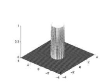
• Dependent sub-Gaussian: $\,2\,$-dimensional isotropic uniform with constant positive density for $\,\|x\|_{2}\leq 1\,$ and $\,0\,$ otherwise.

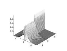
• Dependent super- and sub-Gaussian: $\,1\,$-dimensional Laplacian with density proportional to $\,\exp(-|x_{Lap}|)\,$ and $\,1\,$-dimensional dependent uniform $\,\mathcal{U}(c,c+1)\,$, where $\,c=0\,$ for $\,|x_{Lap}|\leq\log(2)\,$ and $\,c=-1\,$ otherwise.

• Dependent sub-Gaussian:$\,2\,$-dimensional isotropic Cauchy distribution with density proportional to $\,\lambda(\lambda^{2}-x^{2})^{-1}\,$ where $\,\lambda=1\,$.

That means, that the non-normal distributed data are located in a linear subspace.

In the sequel we compare SNGCA with PP and NGCA using the test data sets from above and the estimation error defined in (2.10). Each simulation is repeated $\,100\,$ times. All simulations are done with the hyperbolic tangent index as in  (2.5). Since the speed of convergence varies with the type of non-Gaussian components we use the maximum number $\,maxIter=3\log(d)\,$ of allowed iterations to stop SNGCA. In the experiments the error measure $\,\epsilon(\mathcal{I},\widehat{\mathcal{I}})\,$ is used only to determine the final estimation error. All simulations other than whose w.r.t. model (C) are computed with a componentwise pre-normalization.

(A)	(B)
(C)	(D)
(E)

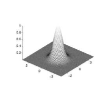
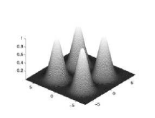
Figure 4.1: densities of the non-Gaussian components: (A) $\,2\,$d independent Gaussian mixtures, (B) $\,2\,$d isotropic super-Gaussian, (C) $\,2\,$d isotropic uniform and (D) dependent $\,1\,$d Laplacian with additive $\,1\,$d uniform, (E) $\,2\,$d isotropic sub-Gaussian

Figure 4.1 illustrates the densities of the non-Gaussian components of the test data. For all numerical experiments reported in this article the dimension of the target space $\,\mathcal{I}\,$ is a priori given as a tuning parameter for the algorithm.

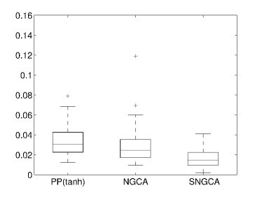
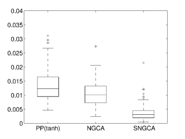
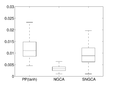
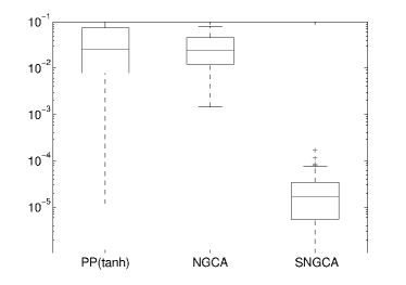
Since the optimizer used in PP tends to trap in a local minima in each of the 100 simulations, PP is 10 times restarted with random starting points. The best result w.r.t. (2.10) is reported as the result of each PP-simulation. In all PP-simulations the number of non-Gaussian dimensions is a priori given. In the next figure 4.2 we present boxplots of the error (2.10) obtained from the methods PP, NGCA and SNGCA.

(A)	(B)
(C)	(D)
(E)

Figure 4.2: performance comparison in $\,10\,$ dimensions of PP and NGCA versus SNGCA (wrt. the error criterion $\,\mathcal{E}(\widehat{\mathcal{I}},\mathcal{I})\,$ ) using the index $\,tanh(x)\,$. The doted line denotes the mean, the solid lines the variance of (2.10).

Concerning the results of SNGCA on the data sets (A) and (D) we observe a slightly inferior performance compared to NGCA. In case of model (A) this is due to the fact that most of the data projections have almost a Gaussian density. Consequently the decrease of the estimation error is slow with increasing number of iterations. In case of the model (D) the higher variance of the results indicate that the initial sampling of the data sets gives a poor result. Consequently more iterations are needed to get an estimation error that is comparable to the result of NGCA. In order to illustrate this interpretation we report in table (4.1) the progress of SNGCA w.r.t. estimation error $\,\varepsilon(\mathcal{I},\widehat{\mathcal{I}})\,$ in each iteration for every test model.

$\,j\,$ $\,\mu_{\epsilon}\,$ $\,\sigma^{2}_{\epsilon}\,$ 1 0.232504 0.045787 2 0.163022 0.072263 3 0.066537 0.032436 4 0.009380 0.021975 5 0.002359 0.000853	$\,j\,$ $\,\mu_{\epsilon}\,$ $\,\sigma^{2}_{\epsilon}\,$ 1 0.30350 0.175313 2 0.144430 0.057856 3 0.088142 0.015168 4 0.041420 0.008197 5 0.026436 0.000917
(A)	(B)
$\,j\,$ $\,\mu_{\epsilon}\,$ $\,\sigma^{2}_{\epsilon}\,$ 1 0.040556 0.004215 2 0.016012 0.002441 3 0.012427 0.001105 4 0.008874 0.000169 5 0.003770 0.000125	$\,j\,$ $\,\mu_{\epsilon}\,$ $\,\sigma^{2}_{\epsilon}\,$ 1 0.203419 0.044672 2 0.023023 0.000314 3 0.019960 0.000211 4 0.012709 0.000197 5 0.009343 0.000127
(C)	(D)
$\,j\,$ $\,\mu_{\epsilon}\,$ $\,\sigma^{2}_{\epsilon}\,$ 1 0.2762e-3 0.1371e-6 2 0.0450e-3 0.0031e-6 3 0.0416e-3 0.0033e-6 4 0.0360e-3 0.0014e-6 5 0.0287e-3 0.0024e-6
(E)

Table 4.1: Progress of SNGCA for test models in $\,10\,$ dimensions with increasing number $\,j\,$ of iterations. The empirical mean of the error $\,\mathcal{E}(\widehat{\mathcal{I}},\mathcal{I})\,$ defined in (2.10) is denoted by $\,\mu_{\epsilon}\,$ and $\,\sigma^{2}_{\epsilon}\,$ is its empirical variance.

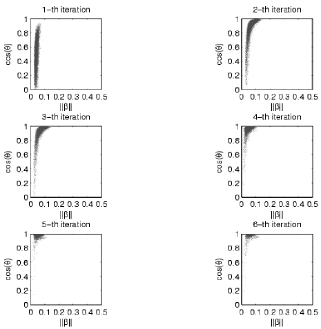
Illustration of one-step-improvement: We shall now illustrate the iterative gain of information about the EDR space. To this end we use the projection of $\,\widehat{\beta}_{j}\,$ to the EDR-space in order to demonstrate, how the algorithm works. Figure 4.3 shows that $\,dist(\widehat{\beta},\widehat{\mathcal{I}})\,$ decreases with increasing number of iterations. We observe, that estimators $\,\widehat{\beta}\,$ with higher norm tend to be close to $\,\mathcal{I}\,$. Nevertheless, this can not be assured for much higher dimensions. Moreover the improvement in each iteration depends on the size of the sampling of measurement directions.

Figure 4.3: illustrative plots of SNGCA applied to toy 20 dimensional data of type (C) (see section 4): We show $\,\|\widehat{\beta}\|\,$ vs. $\,\cos(\theta(\widehat{\beta},\mathcal{I}))\,$ for different iterations of the algorithm where $\,\mathcal{I}\,$ is the a priori known EDR-space.

(A)	(B)
(C)	(D)
(E)

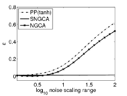
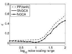
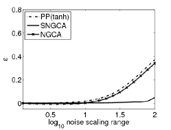
Figure 4.4: results wrt. $\,\mathcal{E}(\widehat{\mathcal{I}},\mathcal{I})\,$ with deviations of Gaussian components following a geometrical progression on $\,[10^{-r},10^{r}]\,$ where $\,r\,$ is the parameter on the abscissa) .

Now let us switch to the question of robustness of the estimation procedure with respect to a bad conditioning of the covariance matrix $\,\Sigma\,$ of the data. In figure 4.4 we consider the same test data sets as above. The non-Gaussian coordinates always have unity variance, but the standard deviation of the $\,8\,$ Gaussian dimensions now follows the geometrical progression $\,10^{-r},10^{-r+2r/7},\ldots,10^{r}\,$ where $\,r=1,\ldots,8\,$. Again we apply a componentwise normalization procedure to the data from the models (A), (B), (D), (E). We observe that the condition of the covariance matrix heavily influences the estimation error for the methods NGCA and PP(tanh). In comparison SNGCA is independent of differences in the noise variance along different directions in most cases. Only the detection of the uniform distribution by SNGCA is influenced by the condition of $\,\Sigma\,$.

(A)	(B)
(C)	(D)
(E)

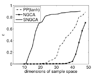
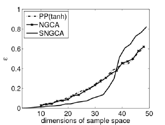
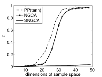
Figure 4.5: results wrt. $\,\mathcal{E}(\widehat{\mathcal{I}},\mathcal{I})\,$ with increasing number of gaussian components.

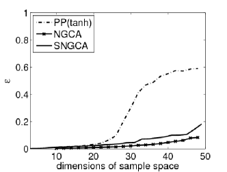
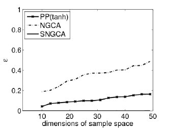
Figure 4.5 compares the behavior of SNGCA with PP and NGCA as the number of standard and homogeneous Gaussian dimensions increases. As described above we use the test models with $\,2\,$-dimensional non-Gaussian components with unity variance. We plot the mean of errors $\,\varepsilon(\widehat{\mathcal{I}},\mathcal{I})\,$ over $\,100\,$ simulations w.r.t. the test models (A) to (E).

Again concerning the mean of errors $\,\varepsilon(\widehat{\mathcal{I}},\mathcal{I})\,$ over $\,100\,$ simulations of PP and NGCA we find a transition in the error criterion to a failure mode for the test models (A), (C) between $\,d=30\,$ and $\,d=40\,$ and between $\,d=20\,$ and $\,d=30\,$ respectively. For the test models (B),(D) and (E) we found a relative continuous increase in $\,\varepsilon(\widehat{\mathcal{I}},\mathcal{I})\,$ for the methods PP and NGCA. In comparison SNGCA fails to analyze test model (A) independently from the size of the sampling, if the dimension exceeds $\,d=12\,$. Concerning test model (B) there is a sharp transition in the simulation result between $\,d=35\,$ and $\,d=40\,$.

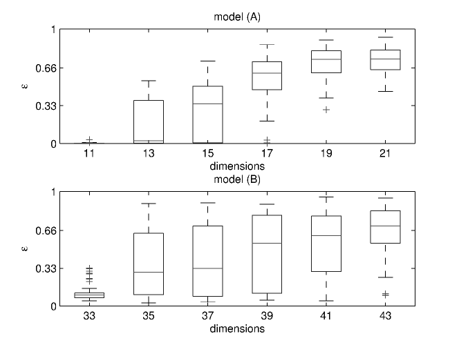
Failure modes: In order to provide a better insight into the details of the failure modes we present box plots of $\,\varepsilon(\widehat{\mathcal{I}},\mathcal{I})\,$ in the transition phases w.r.t. the models (A) and (B).

Figure 4.6: failure modes of SNGCA - upper figure: model (A) - lower figure: model(B)

Figure 4.6 demonstrates the differences in the transition phases of model (A) and (B) respectively. The transition phase is characterized by a high variance of the estimation error. For model (A) the increase of the variance $\,\sigma^{2}_{\varepsilon}\,$ of $\,\varepsilon(\widehat{\mathcal{I}},\mathcal{I})\,$ beginning at dimensions $\,13\,$ and its decrease beginning at dimension $\,15\,$ indicates that a sharp transition phase happens in the interval $\,[13,15]\,$. For higher dimensions more iterations of SNGCA have a decreasing effect on the estimation result. This indicates that by the sampling of the measurement directions, we can not detect the non-Gaussian components of the data density. For model (B) the transition phase starts at dimension $\,35\,$ and ends at dimension $\,43\,$.

Moreover the decrease of $\,\sigma^{2}_{\varepsilon}\,$ towards higher dimensions and the increase of the mean of $\,\varepsilon(\widehat{\mathcal{I}},\mathcal{I})\,$ is much slower. This indicates that the non-Gaussian density components might be detectable if we would allow much more iterations of SNGCA and an enlarged size of the set of measurement directions. This observation motivates the interpretation that the Monte-Carlo sampling of the measurement directions is a very poor strategy that fails to provide sufficient information about the Laplace distribution in high dimensions. Currently the SNGCA performance is limited by the sampling strategy.

4.2 Application to real life examples

We consider a simulating of a mixture of oil and gas flowing under high pressure through a pipeline. Under these physical conditions different phases of the oil-gas-mixture may exist at the same time in the phase space $\,\Gamma\,$. Only some of these phase configurations in $\,\Gamma\,$ are stable over long periods of time. Consequently one expects some clusters of points in $\,\Gamma\,$ indicating the physical state of the mixture. The $\,12\,$-dimensional data set, obtained by numerical simulations of a stationary physical model, was already used before for testing techniques of dimension reduction [3]. The data set comes with a subset of training data and a subset of test data. The length of the time series is $\,1000\,$ in each dimension.

The task with this data is to find the clusters representing the stable configurations in the training data set. It is not known a priori if some dimensions are more relevant than others. However it is known a priori that the data is divided into $\,3\,$ classes, indicated by different shapes of the data points. The cluster information is not used in finding the EDR-space. Again we compare SNGCA with NGCA and PP using the hyperbolic tangent index  (2.5). For PP and NGCA the results are shown in figure 4.7. They were already published in [24].

Figure 4.7: left: 2D projection of the ”oil flow” data manually chosen from 3D projection obtained from by vanilla FastICA methods using the tanh index - right: projection obtained by NGCA using a combination of Fourier, tanh, Gauss-pow3 indices

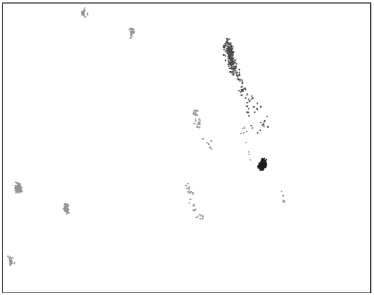
Figure 4.7 shows a slice through $\,\Gamma\,$ such that the structure in the data set becomes visible: Using NGCA we can distinguish $\,10-11\,$ clusters versus at most $\,5\,$ for PP with index  (2.5).

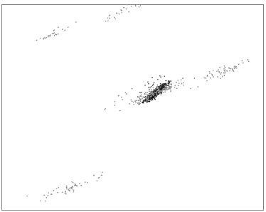
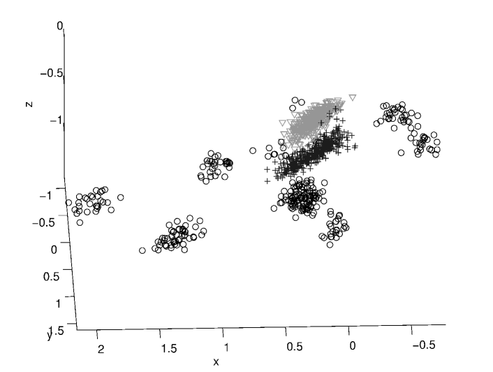
For the SNGCA method the results are shown in the figure 4.8. SNGCA identifies 3 non-Gaussian dimensions. All figures are rotated by hand such that the separation of the cluster is illustrated at best. The next figure 4.8 shows the result of the oil-flow data obtained from SNGCA using a combination of the indices  (2.5) and  (2.6).

Figure 4.8: phase configurations of the ”oil flow” data with apriori cluster mapping induced by crosses, circles and triangles obtained by SNGCA using a combination of asymmetric-Gauss and the tanh index

In this case we can distinguish $\,10-11\,$ clusters versus at most $\,5\,$ for PP. Moreover we confirm the result of NGCA on the data set. The clusters are clearly separated from each other on the SNGCA projection. Only on the PP projection they are partially confounded in one single cluster. By applying the projection obtained from SNGCA to the test data, we found the cluster structure to be relevant. We conclude that SNGCA gives a more relevant estimation of $\,\mathcal{I}\,$ than PP. However it is found that the family of functions $\,h_{\omega}(x)\,$ is an important tuning parameter in SNGCA: If we use only the tanh-index, we found only 6-7 cluster are identified and they are partially confounded. Hence a combination should be used in order to cope with symmetric data distributions.

5 Conclusion

We propose a new improved methodology for the non-Gaussian component analysis, as proposed in [24]. As well as NGCA the suggested method is based on a semi-parametric framework for separation an uninteresting multivariate Gaussian noise subspace from a linear subspace, where the data are non-Gaussian distributed. Both methods assume that the non-Gaussian contribution to the data density contains the structure in a given data set. The combined strategy of convex projection and structural adaptation provides promising results of SNGCA. Moreover SNGCA provides an estimate for the dimension of the non-Gaussian subspace. On the other hand, the quality and the numerical complexity of Monte-Carlo sampling of the measurement directions is the main limitation of the proposed technique.

Appendix A Statistical tests

In this section we shortly report the statistical tests on normality used the dimension reduction step of SNGCA.

In order to detect a significant asymmetry in the distribution of the original data projected on the semi-axis of the numerical approximation of the rounding ellipsoid $\,\mathcal{E}_{\sqrt{d}}\,$ we use the $\,K^{2}\,$-test according to D’Agostino-Pearson [31]. The D’Agostino-Pearson test computes how far the empirical skewness and kurtosis of the given data distribution differs from the value expected with a Gaussian distribution. The test statistic is approximately distributed according to the $\,\chi^{2}_{2}\,$-distribution and its empirical data counterpart is given by

$$\widehat{K}^{2} = \mathcal{Z}^{2}(\sqrt{b_{1}})+\mathcal{Z}^{2}(b_{2})$$

$$\sqrt{b_{1}} = \frac{1}{N}\sum_{i=1}^{N}[\sigma^{-1}(X_{i}-\mu)]^{3}$$

$$b_{2} = \frac{1}{N}\sum_{i=1}^{N}[\sigma^{-1}(X_{i}-\mu)]^{4}$$

Here $\,\mu\,$ denotes the empirical mean, $\,\sigma\,$ the empirical standard deviation of the data and $\,\mathcal{Z}(\cdot)\,$ denotes a normalizing transformations of skewness and kurtosis. The test is more powerful w.r.t. an asymmetry of a distribution.

Furthermore we use the EDF-test according to Anderson-Darling [1] with the modification of Stephens [25]: Let $\,F_{N}\,$ be the empirical cumulative distribution function and $\,F\,$ the assumed theoretical cumulative distribution function. The test statistics $\,\mathcal{T}\,$ measures the quadratic deviations between $\,F_{N}\,$ and $\,F\,$:

$$\mathcal{T}=\int_{\mathbb{R}}[F_{N}(x)-F(x)]^{2}\nu(x)\;dF$$

where $\,\nu(x)\,$ is the weighting function $\,\nu(x)=[F_{N}(x)(1-F_{N}(x))]^{-1}\,$. In sum the data counterpart of $\,\mathcal{T}\,$ is given by

$$\widehat{\mathcal{T}}= -cN-c\sum_{i=1}^{N}N^{-1}(2i-1)[\log(F(\sigma^{-1}(X_{i}-\mu))$$

$$+\log(1-F(\sigma^{-1}(X_{N-i+1}-\mu))]$$

where $\,c=1+0.75N^{-1}+2.25N^{-2}\,$. Again $\,\mu\,$ is the empirical mean and $\,s\,$ the empirical standard deviation of the data. We compute $\,\widehat{\mathcal{T}}\,$ to detect deviations from normality in the tails of the projected distributions. The test is rejected if $\,\widehat{\mathcal{T}}\,$ exceeds a critical value $\,cv\,$ specific for a given level of significance:

$\,\alpha\,$ :	$\,0.10\,$	$\,0.05\,$	$\,0.025\,$	$\,0.01\,$	$\,0.005\,$
$\,cv\,$ :	$\,0.631\,$	$\,0.752\,$	$\,0.873\,$	$\,1.035\,$	$\,1.159\,$

The last test, applied to the projected data is the Shapiro-Wilks test [22] based on a regression strategy in the version given by Royston [20, 21]:

$$W = \sigma^{-1}[1-b^{2}(\sigma^{2}(N-1))^{-1}]^{\lambda}\sim\mathcal{N}(\mu,1)$$

$$b = \sum_{i=1}^{N/2}a_{N-i+1}(X_{N-i+1}-x_{i})$$

$$(a_{1},\dots,a_{N}) = {m^{\top}\Sigma^{-1}\over(m^{\top}\Sigma^{-1^{\top}}\Sigma^{-1}m)^{1/2}}$$

In this test $\,m=(m_{1},\ldots,m_{n})\,$ denotes the expected values of standard normal order statistics for a sample of size $\,N\,$ and $\,\Sigma\,$ is the corresponding covariance matrix.

Appendix B Proofs

B.1 Proof of Theorem 2

We use the following result from the empirical process theory (similar statements under slightly different assumptions can be found e.g. in [26]). Let $\,\mathcal{B}\,$ stand for the unit Euclidean ball, centered at the origin. Similarly, $\,B(\mu,\omega^{\circ})=\{\omega:\|\omega-\omega^{\circ}\|_{2}\leq\mu\}\,$ is a ball of radius $\,\mu\,$ centered at $\,\omega^{\circ}\,$. For a function $\,q(\omega,x)\,$, denote $\,I\!\!E_{N}[q(\omega,X)]=N^{-1}\sum_{i=1}^{N}q(\omega,X_{i})\,$.

Lemma 1.

Let $\,q(\omega,x)\,$ be a continuously differentiable function of $\,\omega\in\mathcal{B}_{d}\,$ and $\,x\in\mathbb{R}^{d}\,$ such that for every $\,\omega\in\mathcal{B}_{d}\,$

$$\operatorname{Var}\bigl{[}q(\omega,X)\bigr{]}\leq q^{*},\quad\operatorname{Cov}\bigl{[}\nabla_{\omega}q(\omega,X)\bigr{]}\leq q^{*}I,$$ (B.12)

with some $\,q^{*},q^{*}>0\,$. Define

$$\zeta(\omega)=N^{1/2}\bigl{\{}I\!\!E_{N}[q(\omega,X)]-I\!\!E[q(\omega,X)]\bigr{\}}$$

and $\,\zeta(\omega,\omega^{\prime})=\zeta(\omega)-\zeta(\omega^{\prime})\,$. Then for any $\,\mathfrak{n}_{0}>1\,$, there is $\,\lambda^{*}_{1}=\lambda^{*}_{1}(\mathfrak{n}_{0})>0\,$ such that for any $\,\omega^{\circ}\in\mathcal{B}_{d}\,$, $\,\mu\leq 1\,$, and $\,\lambda\leq\lambda^{*}_{1}N^{1/2}\,$

$$\log I\!\!E\exp\bigl{[}\lambda\zeta(\omega^{\circ})\bigr{]}\!\!\! \leq \!\!\!\mathfrak{n}_{0}q^{*}\lambda^{2}/2,$$ (B.13)

$$\log I\!\!E\exp\Bigl{[}\frac{\lambda}{\mu}\sup_{\omega\in B(\mu,\omega^{\circ})}\zeta(\omega,\omega^{\circ})\Bigr{]}\!\!\! \leq \!\!\!2\mathfrak{n}_{0}q^{*}\lambda^{2}+\mathfrak{e}_{d}\,,\qquad$$ (B.14)

where $\,\mathfrak{e}_{d}=\sum_{k=1}^{\infty}2^{-k}\log(2^{kd})=4d\log 2\,$. Moreover, define

$$\mathfrak{z}(\lambda)=\mathfrak{n}_{0}\bigl{(}q^{*}/2+2q^{*}\bigr{)}\lambda^{2}+\mathfrak{e}_{d}.$$

Then for any $\,\varepsilon>0\,$

$$I\!\!P\biggl{(}\sup_{\omega\in\mathcal{B}_{d}}\zeta(\omega)\geq 2\lambda^{-1}\bigl{[}\mathfrak{z}(\lambda)+\log\varepsilon^{-1}\bigr{]}\biggr{)}\leq\varepsilon.$$

Proof.

Define for $\,\omega\in\mathcal{B}_{d}\,$

$$g_{0}(\lambda;\omega)=\log I\!\!E\exp\Big{[}\frac{\lambda}{\sqrt{\mathfrak{n}_{0}q^{*}}}\bigl{\{}q(\omega,X_{1})-I\!\!E[q(\omega,X_{1})]\bigr{\}}\Big{]}.$$

Then $\,g_{0}(\lambda;\omega)\,$ is analytic in $\,\lambda\,$ and satisfies $\,g_{0}(0;\omega)=g^{\prime}_{0}(0;\omega)=0\,$. Moreover, the condition (B.12) implies $\,g^{\prime\prime}_{0}(0;\omega)<1\,$. Therefore, there is some $\,\lambda^{*}_{1}>0\,$ such that for any $\,\lambda_{1}\leq\lambda^{*}_{1}\,$ and any unit vector $\,\omega\,$, it holds $\,g_{0}(\lambda_{1};\omega)\leq\lambda_{1}^{2}/2\,$. Independence of the $\,X_{i}\,$’s implies (B.13) for $\,\lambda\leq\lambda^{*}_{1}N^{1/2}(\mathfrak{n}_{0}q^{*})^{-1/2}\,$. In the same way, for $\,\omega,u\in\mathcal{B}_{d}\,$ define $\,\zeta(\omega,X)=\nabla_{\omega}q(\omega,X_{1})-I\!\!E[\nabla_{\omega}q(\omega,X_{1})]\,$ and

$$g(\lambda;\omega,u)=\log I\!\!E\exp\big{[}\frac{2\lambda u^{\top}}{\sqrt{\mathfrak{n}_{0}q^{*}}}\zeta(\omega,X_{1})\big{]}.$$

Then similarly to the above, the function $\,g(\lambda;\omega,u)\,$ is analytic in $\,\lambda\,$ and satisfies with some $\,\lambda^{*}_{1}>0\,$, any $\,\lambda_{1}\leq\lambda^{*}_{1}\,$ and any unit vectors $\,u\,$ and $\,\omega\,$

$$g(\lambda_{1};\omega,u)\leq 2\lambda_{1}^{2}.$$

The bound (B.14) is derived from [23], Lemma 5.1. Independence of the $\,X_{i}\,$’s yields for $\,\lambda\leq\lambda^{*}_{1}N^{1/2}(\mathfrak{n}_{0}q^{*})^{-1/2}\,$

$$\log I\!\!E\exp\biggl{\{}\frac{2\lambda}{\sqrt{\mathfrak{n}_{0}q^{*}}}u^{\top}\nabla\zeta(\omega)\biggr{\}}\leq 2\lambda^{2}.$$

This means that the condition $\,(\mathscr{E}D)\,$ of [23] is verified and the result (B.14) follows from [23], Lemma 5.1. Introduce a random set $\,A=\{(\lambda/2)\sup_{\omega}\zeta(\omega)>\mathfrak{z}(\lambda)+\log\varepsilon^{-1}\}\,$. and $\,A^{c}\,$ is its complement. By the Cauchy-Schwartz inequality

$$I\!\!P(A^{c})\!\!\! \leq \!\!\!I\!\!E\exp\biggl{\{}\frac{\lambda}{2}\sup_{\omega}\zeta(\omega)-\mathfrak{z}(\lambda)-\log\varepsilon^{-1}\biggr{\}}$$

$$\leq \!\!\!\varepsilon I\!\!E^{1/2}\exp\bigl{\{}\lambda\zeta(\omega^{\circ})-\mathfrak{n}_{0}q^{*}\lambda^{2}/2\bigr{\}}$$

$$\!\!\!\times\,I\!\!E^{1/2}\exp\bigl{\{}\lambda\sup_{\omega}\zeta(\omega,\omega^{\circ})-2\mathfrak{n}_{0}q^{*}\lambda^{2}-\mathfrak{e}_{d}\bigr{\}}\leq\varepsilon$$

and the last result follows.
∎

The result of Lemma 1 can be easily extended to the case of a vector function $\,q(\omega,x)\in\mathbb{R}^{d}\,$:

$$I\!\!P\biggl{(}\sup_{\omega\in\mathcal{B}_{d}}\|\zeta(\omega)\|_{\infty}\geq 2\lambda^{-1}\bigl{[}\mathfrak{z}(\lambda)+\log(d/\varepsilon)\bigr{]}\biggr{)}\leq\varepsilon.$$

This fact can be obtained by applying Lemma 1 to each component of the vector $\,\zeta(\omega)\,$. The term $\,\log(d/\varepsilon)\,$ is responsible for the overall deviation probability.

Let now $\,f(x,\omega)\,$ be a twice continuously differentiable function of $\,\omega\in\mathcal{B}_{d}\,$ and $\,x\in\mathbb{R}^{d}\,$ such that for every $\,j\leq d\,$, $\,\omega\in\mathcal{B}_{d}\,$, and $\,x\in\mathbb{R}^{d}\,$, it holds

$$\operatorname{Var}\bigl{[}X_{j}\,f(X,\omega)\bigr{]}\leq f^{*}_{1},\quad\operatorname{Cov}\bigl{[}X_{j}\,\nabla_{\omega}f(X,\omega)\bigr{]}\leq f^{*}_{1}I,$$

$$\operatorname{Var}\biggl{[}\frac{\partial}{\partial x_{j}}f(X,\omega)\biggr{]}\leq f^{*}_{1},\quad\operatorname{Cov}\biggl{[}\nabla_{\omega}\frac{\partial}{\partial x_{j}}f(X,\omega)\biggr{]}\leq f^{*}_{1}I,$$

Then for any $\,\mathfrak{n}_{0}>1\,$, there is $\,\lambda^{*}_{1}=\lambda^{*}_{1}(\mathfrak{n}_{0})>0\,$ and for any $\,\varepsilon>0\,$, a random set $\,A\,$ with $\,I\!\!P(A)\geq 1-\varepsilon\,$ such that on $\,A\,$ it holds by Lemma 1

$$\sup_{\omega\in\mathcal{B}_{d}}\big{\|}I\!\!E_{N}[Xf(X,\omega)]-I\!\!E[Xf(X,\omega)]\big{\|}_{\infty}\leq\delta_{N},$$

$$\sup_{\omega\in\mathcal{B}_{d}}\big{\|}I\!\!E_{N}[\nabla_{x}f(X,\omega)]-I\!\!E[\nabla_{x}f(X,\omega)]\big{\|}_{\infty}\leq\delta_{N},$$

where

$$\delta_{N}=N^{-1/2}\inf_{\lambda\leq\lambda^{*}_{1}N^{1/2}}\bigl{\{}5\mathfrak{n}_{0}f^{*}_{1}\lambda+2\lambda^{-1}\bigl{[}\mathfrak{e}_{d}+\log(2d/\varepsilon)\bigr{]}\bigr{\}}.$$

By construction of vectors $\,\widehat{\gamma}_{l}\,$ and $\,\widehat{\eta}_{l}\,$, it holds on $\,A\,$

$$\max_{1\leq l\leq L}\|\widehat{\gamma}_{l}-\gamma_{l}\|_{\infty}\leq\delta_{N},\quad\max_{1\leq l\leq L}\|\widehat{\eta}_{l}-\eta_{l}\|_{\infty}\leq\delta_{N}\,.$$

This implies for any $\,\|c\|_{1}\leq 1\,$

$$\|\widehat{\gamma}(c)-\gamma(c)\|_{\infty}\leq\delta_{N},\;\;\;\|\widehat{\eta}(c)-\eta(c)\|_{\infty}\leq\delta_{N}.$$

The constraint $\,\widehat{\gamma}(\widehat{c})=0\,$ implies $\,\|\gamma(\widehat{c})\|_{\infty}\leq\delta_{N}\,$, thus

$$\|\gamma(\widehat{c})\|_{2}\leq\sqrt{d}\,\delta_{N},$$

and by  (2.3)

$$\bigl{\|}(I-\Pi^{*})\widehat{\eta}(\widehat{c})\bigr{\|}_{2}$$

$$\leq \bigl{\|}(I-\Pi^{*})\{\widehat{\eta}(\widehat{c})-{\eta}(\widehat{c})\}\bigr{\|}_{2}+\bigl{\|}(I-\Pi^{*})\eta(\widehat{c})\bigr{\|}_{2}$$

$$\leq \bigl{\|}\widehat{\eta}(\widehat{c})-\eta(\widehat{c})\bigr{\|}_{2}+\bigl{\|}\Sigma^{-1}\gamma(\widehat{c})\bigr{\|}_{2}$$

$$\leq \sqrt{d}\bigl{(}\delta_{N}+\bigl{\|}\Sigma^{-1}\bigr{\|}_{2}\delta_{N}\bigr{)}.$$

B.2 Proof of Theorem 3

Let $\,\mathscr{S}\,$ stand for the convex envelope of $\,\{\pm\widehat{\beta}_{j}\}_{j=1}^{J}\,$. As $\,\mathscr{E}_{1}(B)\,$ is inscribed in $\,\mathscr{S}\,$, its support function $\,\xi_{\mathscr{E}_{1}(B)}(x)=\max_{s\in\mathscr{E}_{1}(B)}s^{\top}x\,$ is majorated by that of $\,\mathscr{S}\,$:

$$\xi_{\mathscr{E}_{1}(B)}(v)\leq\xi_{\mathscr{S}}(v)=\max_{j=1,...,J}|v^{\top}\widehat{\beta}_{j}|,\;\;\mbox{for any}\;\;v\in\mathbb{R}^{d}.$$

Next, the support function of the ellipsoid $\,\mathscr{E}_{1}(B)\,$ is

$$\xi_{\mathscr{E}_{1}(B)}(v)=(v^{\top}B^{-1}v)^{1/2},$$

so that the condition $\,\|\widehat{\beta}_{j}-\beta_{j}\|_{2}\leq\varrho\,$ implies

$$v^{\top}B^{-1}v\leq\max_{j=1,...,J}|v^{\top}\widehat{\beta}_{j}|^{2}\leq\varrho^{2},$$

for any $\,v\perp\mathcal{I}\,$.

Let us prove the second claim of the proposition. Let $\,\Pi^{*}\,$ be a projector onto $\,\mathcal{I}\,$. By the assumption of the proposition there exist coefficients $\,\mu_{j}\,$ with $\,\sum_{j}\mu_{j}\leq 1\,$ such that

$$S\stackrel{{\scriptstyle\operatorname{def}}}{{=}}\frac{1}{2}\biggl{[}\sum_{j}\mu_{j}\beta_{j}\beta_{j}^{\top}-2\varrho^{2}\Pi^{*}\biggr{]}\succeq 0.$$

This implies (2.11). Now, for any such $\,S\,$ and its pseudo-inverse $\,S^{+}\,$, the ellipsoid, $\,\mathscr{E}^{f}_{1}(S^{+})\,$ with

$$\mathscr{E}^{f}_{1}(S^{+})=\{x\in\mathcal{I}\mid x^{\top}S^{+}x\leq 1\}$$

is inscribed into $\,\mathscr{S}\,$. Indeed, the support function $\,\xi_{\mathscr{E}^{f}_{1}(S^{+})}(x)=(x^{\top}Sx)^{1/2}\,$ of this ellipsoid fulfills for $\,x\in\mathcal{B}_{d}\,$

$$\xi_{\mathscr{E}^{f}_{1}(S^{+})}(x) \leq \biggl{(}\sum_{j}\mu_{j}\Bigl{[}\frac{1}{2}(x^{\top}\beta_{j})^{2}-\varrho^{2}\Bigr{]}\biggr{)}^{1/2}$$

$$\leq \biggl{(}\sum_{j}\mu_{j}\bigl{|}x^{\top}\widehat{\beta}_{j}\bigr{|}^{2}\biggr{)}^{1/2}$$

$$\leq \max_{1\leq j\leq J}|x^{\top}\widehat{\beta}_{j}|=\xi_{\mathscr{S}}(x),$$

Now we are done: as the ellipsoid $\,\mathscr{E}^{f}_{1}(S^{+})\,$ is inscribed into $\,\mathscr{S}\,$, it is contained in the concentric to $\,\mathscr{E}_{1}(B)\,$ ellipsoid $\,\mathscr{E}_{\sqrt{d}}(B)\,$ which covers $\,\mathscr{S}\,$.

To show the last statement of the theorem, observe that

$$\mathrm{Tr}\bigl{[}(\widehat{\Pi}-\Pi^{*})^{2}\bigr{]}=2(m-\mathrm{Tr}[\Pi^{*}\widehat{\Pi}])=2\mathrm{Tr}\bigl{[}(I-\Pi^{*})\widehat{\Pi}\bigr{]}.$$

On the other hand, using the second claim one gets

$$\mathrm{Tr}\bigl{[}(I-\Pi^{*})\widehat{\Pi}\bigr{]} \leq (d-m)\sup_{v\perp\mathcal{I}}v^{\top}\widehat{\Pi}v$$

$$\leq (d-m)\sup_{v\perp\mathcal{I}}\frac{v^{\top}B^{-1}v}{\lambda_{m}(B^{-1})}$$

$$\leq \frac{2d^{3/2}\varrho^{2}}{\lambda^{*}-2\varrho^{2}}.$$

Appendix C The algorithm

Here we present the full algorithmic description of the SNGCA procedure. We start with the linear estimation subprocedure:

Data: $\,Y\,$,$\,L\,$,$\,J\,$

Result: $\,\{\widehat{\beta}_{j}\}_{j=1}^{J}\,$

Sampling: choice of measurement directions

for j=1 to J do  for l=1 to L do  Compute:

$\,\widehat{\eta}_{jl}=N^{-1}\sum_{i=1}^{N}\nabla h_{\omega_{jl}}(Y_{i})\,$

$\,\widehat{\gamma}_{jl}=N^{-1}\sum_{i=1}^{N}Y_{i}h_{\omega_{jl}}(Y_{i})\,$

end Compute $\,\widehat{c}_{j}\,$ as in  (2.8) and $\,\widehat{\beta}_{j}=\sum_{l=1}^{L}\widehat{c}_{j}\widehat{\eta}_{jl}\,$.

end

Algorithm 4 (linear estimation of $\,\beta(\psi_{h,c})\,$).

The following subprocedure reports the computation of the $\sqrt{d}$-rounding ellipsoid based on a proposal in [18]:

Data: $\,\{\widehat{\beta}_{j}\}_{j=1}^{J}\,$

Result: $\,\widehat{B}\,$,

Let $\,\delta_{i}^{k^{\ast}}=\max_{1\leq j\leq J}\;\langle\widehat{\beta}_{j},\widehat{B}_{i}\widehat{\beta}_{j}\rangle\,$ and set $\,\nu_{i}=\delta_{i}^{k^{\ast}}d^{-1}\,$.

Let $\,\widehat{B}_{0}\,$ be the inverse empirical covariance matrix of the

$\,\widehat{\beta}_{j}\,$ and set $\,t_{i}=\nu_{i}(\delta_{i}^{k^{\ast}}d^{-1}-1)^{-1}\,$.

Moreover let $\,i\,$ be the loop index.

repeat  $\,x_{i}=\widehat{B}_{i}\widehat{\beta}_{k^{\ast}}\,$

$\,\widehat{B}_{i+1}=(1-t_{i})^{-1}\Big{(}\widehat{B}_{i}-t_{i}(1+\nu_{i})^{-1}x_{i}x_{i}^{\top}\Big{)}\,$

$\,\delta_{i+1}^{k^{\ast}}=(1-t_{i})^{-1}\Big{(}\delta_{i}^{k^{\ast}}-t_{i}(1+\nu_{i})^{-1}\langle\widehat{\beta}_{k^{\ast}},x_{i}\rangle^{2}\Big{)}\,$

until $\,\delta_{i}^{k^{\ast}}\leq C\cdot d\,$ where $\,C\,$ is a tuning parameter.

Algorithm 5 (Compute of the $\,\sqrt{d}\,$-rounding of the MVEE).

The next algorithm 6 reports the pseudocode for constructing a reduced basis of the target space from the estimated elements by means of algorithm 5:

Data: $\,\widehat{B}\,$

Result: $\,\big{\langle}\text{first }m\text{ eigenvectors of }\widehat{B}\big{\rangle}\,$

Let $\,\widehat{V}\,$ be the matrix of eigenvectors $\,\widehat{v}_{i}\,$ from $\,\widehat{B}\,$

computed according to algorithm 5.

for i=1 to d do  Project the data orthogonal on $\,\widehat{v}_{i}\,$.

Compute tests on normality of the projected data.

end Discard every eigenvector with associated normal

distributed projected data.

Algorithm 6 (Dimension Reduction).

In algorithm 4 we start with a random initialization of the non-parametric estimator $\,\widehat{\beta}_{j}\,$ by means of a Monte-Carlo sampling of the directions $\,\omega_{jl}\,$ and $\,\xi_{j}\,$. However we can use the result of the first iteration $\,k=1\,$ of SNGCA in order to accumulate information about $\,\mathcal{I}\,$ in a sequence $\,\widehat{\mathcal{I}}_{1},\widehat{\mathcal{I}}_{2},\ldots\,$ of estimators of the target space. The procedure is described in detail in algorithm 7.

Data: $\,\big{\langle}\text{first }m\text{ eigenvectors of }\widehat{B}\big{\rangle}\,$

Let $\,\{\widehat{v_{i}}\}_{i=1}^{m}\,$ denote the reduced set of eigenvectors from

$\,\widehat{B}\,$ and let $\,k\,$ iterations be completed. To initialize iteration $\,k+1\,$ choose random numbers $\,z_{j1},\ldots,z_{jm}\,$

and $\,u_{l1},\ldots,u_{lm}\,$ from $\,\mathcal{U}_{[-1,1]}\,$ and set

$\,\quad\quad\quad\xi_{j}:=\sum_{s=1}^{m}z_{js}\widehat{v}_{i_{s}}\mbox{ for }1\leq j\leq n_{1}<J\,$

$\,\quad\quad\quad\omega_{l}:=\sum_{s=1}^{m}u_{ls}\widehat{v}_{i_{s}}\mbox{ for }1\leq l\leq n_{2}<L\,$

Then define $\,\omega_{L-n_{2}},\ldots,\omega_{L}\,$ and $\,\xi_{J-n_{1}},\ldots,\xi_{J}\,$ analogous to the case $\,k=1\,$. Now compose the sets

$\,\quad\quad\quad\{\xi_{1}^{(k)},\ldots,\xi_{n_{1}}^{(k)},\xi_{n_{1}+1}^{(k)},\ldots,\xi_{J}^{(k)}\}\,$

$\,\quad\quad\quad\{\omega_{1}^{(k)},\ldots,\omega_{n_{2}}^{(k)},\omega_{n_{2}+1}^{(k)},\ldots,\omega_{L}^{(k)}\}\,$

For the initialization in the case $\,k=k+1\,$. Moreover we choose $\,n_{1}=kd\,$ and $\,n_{2}=kd\,$ until $\,n_{1}>J-d\,$ or $\,n_{2}>L-d\,$. Otherwise set $\,n_{1}=J-d\,$ or $\,n_{2}=L-d\,$.

Algorithm 7 (structural adaptation of the linear estimation ).

Choice of parameters: One of the advantages of the algorithm proposed above is the fact that there are only a few tuning parameters.

• Suppose now that $\,\omega_{i}\,$ is an absolute continuous random variable with $\,\omega_{i}\sim\mathcal{U}_{[-1,1]}\,$. Without loss of generality we set $\,e=(1,0,\ldots,0)\,$. Due to the normalization of $\,(\omega_{1},\ldots,\omega_{d})\,$, it holds:

  $$I\!\!P\big{(}|(\omega_{1},\ldots,\omega_{d})^{\top}e|\geq 0.5\big{)}=\big{(}\sqrt{d}\big{)}^{-1}$$

  However the choice of $\,J\,$ and $\,L\,$ heavily depends on the non-gaussian components. In the experiments we use $\,7d\leq J\leq 18d\,$ and $\,6d\leq L\leq 16d\,$.

• Set the parameter of the stopping rule to $\,\delta=0.05\,$.

• Set the constant in the stopping rule for the computation of the MVEE to $\,C=2\,$.

• Set the significance level of the statistical tests to $\,\alpha=0.05\,$.
  

Finally we give a description of the complete algorithm.

Data: $\,\{X_{i}\}_{i=1}^{N}\,$,$\,L\,$,$\,J\,$,$\,\alpha\,$

Result: $\,\widehat{\mathcal{I}}\,$

Normalization: The data $\,(X_{i})_{i=1}^{N}\,$ are recentered. Let

$\,\sigma=(\sigma_{1},\ldots\sigma_{d})\,$ be the standard deviations of the

components of $\,X_{i}\,$. Then $\,Y_{i}=\mathrm{diag}(\sigma^{-1})X_{i}\,$ denotes the

componentwise empirically normalized data.

Main Procedure:;  // loop on $\,k\,$

while $\,\sim StoppingCriterion(\mathcal{I},\widehat{\mathcal{I}})\,$ do  Sampling: The components of the Monte-Carlo-parts

of $\,\xi_{j}^{(k)}\,$ and $\,\omega_{jl}^{(k)}\,$ are randomly chosen from $\,\mathcal{U}_{[-1,1]}\,$.

The other part of the measurement directions are

initialized according to the structural adaptation

approach described in algorithm 7. Then $\,\xi_{j}^{(k)}\,$ and

$\,\omega_{jl}^{(k)}\,$ are normalized to unit length.

Linear Estimation Procedure:

for j=1 to J do  for l=1 to L do  $\,\widehat{\eta}_{jl}^{(k)}=N^{-1}\sum_{i=1}^{N}\nabla h_{\omega_{jl}^{(k)}}(Y_{i})\,$

$\,\widehat{\gamma}_{jl}^{(k)}=N^{-1}\sum_{i=1}^{N}Y_{i}h_{\omega_{jl}^{(k)}}(Y_{i})\,$

endCompute the coefficients $\,\{c_{l}\}_{l=1}^{L}\,$ by solving the

second-order conic optimization problem  (2.8):

$\,\quad\quad\quad\quad\quad\min\;q\qquad\mbox{s.t.}\,$

$\,\quad\quad\quad\quad\quad\quad\frac{1}{2}\|z\|_{2}\leq q\,$

$\,\quad\quad\sum_{l=1}^{L}(c_{l}^{+}-c_{l}^{-})\widehat{\eta}_{jl}^{(k)}-z=\xi_{j}^{(k)}\,$

$\,\quad\quad\quad\sum_{l=1}^{L}(c_{l}^{+}-c_{l}^{-})\widehat{\gamma}_{jl}^{(k)}=0\,$

$\,\sum_{l=1}^{L}(c_{l}^{+}-c_{l}^{-})\leq 1,\quad 0\leq c_{l}^{+},c_{l}^{-}\quad\forall l\,$

Compute $\,\widehat{\beta}_{j}^{(k)}=\sum_{l=1}^{L}(\widehat{c}_{l}^{+}-\widehat{c}_{l}^{-})\widehat{\eta}_{jl}^{(k)}\,$

end Dimension Reduction:

Compute the symmetric matrix $\,\widehat{B}^{(k)}\,$ defining the

approximation of $\,\mathcal{E}\,$ according to algorithm 5. Reduce the basis of $\,\mathcal{X}\,$ according to algorithm 6.

end

Algorithm 8 (full procedure of SNGCA).

Complexity: We restrict ourselves to the leading polynomial terms of the arithmetical complexity of corresponding computations counting only the multiplications.

• The numerical effort to compute $\,\eta_{jl}\,$ and $\,\gamma_{jl}\,$ in algorithm 4 heavily depends on the choice of $\,h(\omega^{\top}x)\,$. Let $\,h(\omega^{\top}x)=\tanh(\omega^{\top}x)\,$. Then this step takes $\,\mathcal{O}(J(\log N)^{2}N^{2})\,$ operations.

• Algorithm 5 takes $\,\mathcal{O}(d^{2}J\log(J))\,$ operations [18].

• For the optimization step in 4 we use a commercial solver based on an interior point method. The constrained convex projection solved as an SOCP takes $\,\mathcal{O}(d^{2}n^{3})\,$ operations there $\,n\,$ is the number of constraints.

• Computation of the statistical tests in one dimension: Let $\,N\,$ denote the number of samples. D’Agostino-Pearson-test needs $\,\mathcal{O}(N^{3}\log N)\,$ and the Anderson-Darling-test $\,\mathcal{O}((\log N)^{2}N^{2})\,$ operations. The test of Shapiro-Wilks takes $\,\mathcal{O}(N^{2})\,$. In order to avoid robustness problems [14] the number of samples is limited to $\,N\leq 1000\,$. For larger data sets, $\,N=1000\,$ points are randomly chosen.

Hence without tests $\,\widehat{\mathcal{I}}\,$ is computed in $\,\mathcal{O}(J(\log N)^{2}N^{2}+d^{2}J\log(J)+d^{2}n^{3})\,$ arithmetical operations per iteration.

References

• [1] F.J. Anscombe and W.J. Glynn. Distribution of kurtosis statistic for normal statistics. Biometrika, 70(1):227–234, 1983.
• [2] E. Bura and R. D. Cook. Estimating the structural dimension of regressions via parametric inverse regression. J. Roy. Statist. Soc. Ser. B, 63(393-410), 2001.
• [3] M. Svensen C.M. Bishop and C.K.I. Wiliams. Gtm: The generative topographic mapping. Neural Computation, 10(1):215–234, 1998.
• [4] R.D. Cook. Principal hessian directions revisited. J. Am. Statist. Ass., 93:85–100, 1998.
• [5] T.M. Cover and J.A. Thomas. Elements of Information Theory. Wiley Series in Telecommunications. Wiley and Sons, New York, 1991.
• [6] P. Diaconis and D. Friedman. Asymptotics of graphical projection pursuit. Annals of Statistics, 12(3):793–815, 1984.
• [7] N.E. Goljandina, V.V. Nekrutkin, and A.A. Zhigljavsky. Analysis of Time Series Structure: SSA and related technique. Chapman and Hall (CRS), Boca Raton, 2001.
• [8] T. Hastie, R. Tibshirani, and J. Friedman. The elements of statistical learning. Springer Series in Statistcs. Springer, 2001.
• [9] M. Hristache, A. Juditsky, J. Polzehl, and V. Spokoiny. Structure adaptive approach for dimension reduction. Ann. Statist., 29(6):1537–1566, 2001.
• [10] P. J. Huber. Projection pursuit. The Annals of Statistics, 13(2):435–475, 1985.
• [11] A. Hyvärinen. Survey on independent component analysis. Neural Computing Surveys, 2:94–128, 1999.
• [12] F. John. Extremum problems with inequalities as subsidiary conditions, volume Reprinted in: Fritz John, Collected Papers Volume 2 of Birkhäuser, Boston, pages 543–560. J. Moser, 1985.
• [13] I.T. Jolliffe. Principal Component Analysis. Springer Series in Statistics. Springer, Berlin and New York, 2nd edition, 2002.
• [14] H.C. Thode Jr. Testing for Normality. Marcel Dekker, New York., 2002.
• [15] K.C. Li. Sliced inverse regression for dimension reduction. J. Am. Statist. Ass., 86:316–342, 1991.
• [16] K.C. Li. On principal hessian directions for data visualisation and dimension reduction: another application of stein’s lemma. Ann. Statist., 87:1025–1039, 1992.
• [17] M. Mizuta. Dimension Reduction Methods, chapter 6, pages 566–89. J.E. Gentle and W. Härdle, and Y. Mori (eds.): Handbook of Computational Statistics, 2004.
• [18] Yu. E. Nesterov. Rounding of convex sets and efficient gradient methods for linear programming problems. Discussion Paper 2004-4, CORE, Catholic University of Louvain, Louvain-la-Neuve, Belgium, 2004.
• [19] S. Roweis and L. Saul. Nonlinear dimensionality reduction by locally linear embedding. Science, 290:2323–2326, 2000.
• [20] J.P. Royston. An extension of shapiro and wilks’ w test for normality to large samples. Applied Statistics, 31:115–124, 1982.
• [21] J.P. Royston. The w test for normality. Applied Statistics, 21:176–180, 1982.
• [22] S.S. Shapiro and M.B. Wilk. An analysis of variance test for normality. Biometrika, 52:591–611, 1965.
• [23] V. Spokoiny. A penalized exponential risk bound in parametric estimation. http://arxiv.org/abs/0903.1721, 2009.
• [24] V. Spokoiny, G. Blanchard, M. Sugiyama, M.Kawanabe, and Klaus-Robert Müller. In search of non-Gaussian components of a high-dimensional distribution. Journal of Machine Learning Research, preprint TR05-003, 2005.
• [25] M. A. Stephens. Goodness of Fit Techniques, chapter Tests based on Goodness of Fit. D’Agostino, R. B. and Stephens, M. A., 1986.
• [26] A. van der Vaart and J.A. Wellner. Weak Convergence and Empirical Proccesses. Springer Series in Statistics. Springer – New York, 1996.
• [27] L. Wasserman. All of Nonparametric Statistics. Springer Texts in Statistcs. Springer, 2006.
• [28] H. Wold. Soft Modeling. The Basic Design and Some Extensions., volume 2 of Systems Under Indirect Observation, pages 1–53. K.-G. Jöreskog and H. Wold, North-Holland, Amsterdam, 1982.
• [29] S. Wold, S. Hellberg, M. Sjostrom, and H. Wold. PLS Model Building: Theory and applications. PLS modeling with latent variables in two or more dimensions. 1987.
• [30] Y. Xia, H. Tong, W.K. Li, and Li-Xing Zhu. An adaptive estimation of dimension reduction space. Journal of the Royal Statistical Society, Series B, 64(3):363–388, 2001.
• [31] J.H. Zar. Biostatistical Analysis, (2nd ed.). NJ: Prentice-Hall, Englewood Cliffs., 1999.