Serber symmetry, Large and Yukawa-like One Boson Exchange Potentials
Abstract
The Serber force has relative orbital parity symmetry and requires vanishing NN interactions in partial waves with odd angular momentum. We illustrate how this property is well fulfilled for spin triplet states with odd angular momentum and violated for odd singlet states for realistic potentials but fails for chiral potentials. We analyze how Serber symmetry can be accommodated within a large perspective when interpreted as a long distance symmetry. A prerequisite for this is the numerical similarity of the scalar and vector meson resonance masses. The conditions under which the resonance exchange potential can be approximated by a Yukawa form are also discussed. While these masses arise as poles on the Second Riemann in scattering, we find that within the large expansion the corresponding Yukawa masses correspond instead to a well defined large approximation to the pole which cannot be distinguished from their location as Breit-Wigner resonances.
pacs:
03.65.Nk,11.10.Gh,13.75.Cs,21.30.Fe,21.45.+vI Introduction
The modern theory of nuclear forces Epelbaum et al. (2008) aims at a systematic and model-independent derivation of the forces between nucleons in harmony with the symmetries of Quantum Chromodynamics. Actually, an outstanding feature of nuclear forces is their exchange character. Many years ago, Serber postulated Serber (1938) an interesting symmetry for the nucleon-nucleon system based on the observation that at low energies the proton-proton and neutron-proton differential cross section are symmetric functions in the Center of Mass (CM) scattering angle around . This orbital parity symmetry corresponds to the transformation in the scattering amplitude and was naturally explained by assuming that the potential was vanishing for partial waves with odd angular momentum. Specific attempts were directed towards the verification of such a property Ashkin and Wu (1948) (See Refs. Christian (1952) and Blatt and Weisskopf (1952) for early and comprehensive reviews.). This symmetry was shown to hold for the NN system, up to relatively high energies Christian and Hart (1950). However, such a force was also found to be incompatible with the requirement of nuclear matter saturation Gerjuoy (1950) as well as with the underlying meson forces mediated by one and two pion exchange Nakabayasi and Sato (1952). These puzzling inconsistencies were cleared up when it was understood that only singular Serber forces could provide saturation Jastrow (1951). Old phase shift analyses Hull et al. (1961) confirm the rough Serber exchange character of nuclear forces. Many nuclear structure de la Ripelle et al. (2005), nuclear matter Fetter and Walecka (1971), nuclear reactions Bethe and Longmire (1950); Lashko and Filippov (2007); Ali et al. (1985), use Serber forces both for their simplicity as well as their phenomenological success in the low and medium energy region. The possibility of implementing Serber forces in the nuclear potential was envisaged in Skyrme’s seminal paper Skyrme (1959). Modern versions (SLy4) of the Skyrme effective interactions Chabanat et al. (1997) implement the symmetry explicitly. In a recent paper Zalewski et al. (2008) a novel fitting strategy has been proposed for the coupling constants of the nuclear energy density functional, which focus on single-particle energies rather than ground-state bulk properties, yielding naturally an almost perfect fulfillment of Serber symmetry.
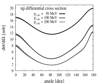
A vivid demonstration of the Serber symmetry is shown in Fig. 1 where the np differential cross section is plotted for several LAB energies using the Partial Wave Analysis and the high quality potentials Stoks et al. (1993, 1994) carried out by the Nijmegen group. While discrepancies regarding the comparison between forward and backward directions show that this symmetry breaks down at short distances, the intermediate region does exhibit Serber symmetry. In any case it is interesting to see that even in the intermediate energy region departures from the symmetry can be seen, the most important one is the fact that the symmetry point is shifted a few degrees towards lower values than for increasing energies. While these are well established features of the NN interaction, it is amazing that such a time honoured force and gross feature of the NN interaction, even if it does not hold in the entire range, has no obvious explanation from the more fundamental and QCD motivated side. To our knowledge this topic has not been explicitly treated in any detail in the literature and no attempts have been made to justify this evident but, so far, accidental symmetry. The present paper tries to fill this gap unveiling Serber symmetry at the relevant scales from current theoretical approaches to the NN problem, looking for its consequences in nuclear physics and analyzing its possible origin. Of course, a definite explanation might finally be given by lattice QCD calculations for which incipient results exist already in the case of S-wave interactions Ishii et al. (2007); Beane et al. (2006).
The motivation for the present study arises from our recent analysis Calle Cordon and Ruiz Arriola (2008a) of an equally old symmetry, the SU(4)-spin-isospin symmetry proposed independently by Wigner and Hund Wigner (1937); Hund (1937) by introducing the concept of long distance symmetry. Specifically we showed how a symmetry of the potential at any non vanishing but arbitrarily small distance does not necessarily imply a symmetry of the S-matrix which may be directly observed at all energies. This provided an interpretation of the role played by the Wigner symmetry in the S-waves; the potentials for the two nucleon and states are identical while the corresponding phase shifts are very different at all measurable energies. Furthermore, we showed how a sum rule for SU(4) super-multiplet phase shifts splitting due to spin-orbit and tensor interactions is well fulfilled for non-central L-even waves, and strongly violated in L-odd waves where a Serber-like symmetry holds instead. In Section II we review the sum rules obtained from our previous work for the partial wave phase shifts and show how their potential counterpart is also well verified by high quality NN potentials, i.e. potentials which have . Obviously, any NN potential explaining the data will necessarily comply to odd-L Serber symmetry as a whole; a less trivial matter is to check whether this is displayed explicitly by the potential and what are the relevant ranges where the symmetry is located. At long distances the interaction is given by One Pion Exchange (OPE) which is Wigner symmetric for even-L waves and provides a violation of Serber symmetry for odd-L waves at long distances. Phenomenological potentials seem to provide different ranges for each symmetry. In Section III we analyze the signatures of the symmetry and its range from several viewpoints including the PWA of the Nijmegen group, the approach and chiral two pion exchange. In Section IV we digress on the meaning of counterterms as a diagnostics tool to characterize a long distance symmetry both from a perturbative as well as from a Wilsonian renormalization point of view, the implications for Skyrme forces and the resonance saturation of chiral forces.
In any case, the evidence for both even-L Wigner and odd-L Serber symmetries is so overwhelming that we feel a pressing need for an explanation more closely based on our current knowledge of strong interactions and QCD. Actually, central to our analysis will be the use of the large expansion ’t Hooft (1974); Witten (1979) (for comprehensive reviews see e.g. Manohar (1998); Jenkins (1998); Lebed (1999)). Here is the number of colours and in this limit the strong coupling constant scales as . For color singlet states the picture is that of infinitely many stable mesons and glue-balls, which masses behave as and widths as , and heavy baryons, with their masses scaling as . This limit also fixes the interactions among hadrons. Meson-meson interactions are weak since they scale as , meson-baryon interactions and baryon-baryon interactions are strong as they scale as . While the pattern of -symmetry breaking complies to the large expectations Kaplan and Savage (1996); Kaplan and Manohar (1997), a somewhat unexpected conclusion, we also pointed out that Serber symmetry, while not excluded for odd-L waves, was not a necessary consequence of large . The search for an explanation of the Serber force requires more detailed information than in the case of Wigner symmetry.
In Section V we approach the Serber symmetry from a large perspective, and make explicit use of the fact that the meson exchange picture seems justified Banerjee et al. (2002). Actually, within such a realization a necessary prerequisite for the validity of the symmetry would be a numerical similarity of the scalar and vector meson masses. This poses a puzzle since, as is well known, these mesons arise as resonances in scattering as poles in the second Riemann sheet yielding the values Caprini et al. (2006) and Amsler et al. (2008). The scalar and vector masses and widths are sufficiently different as to make one question if one is close to the Serber limit. In Section VI we review the role of two pion exchange and analyze the resonances as well as the generation of Yukawa potentials from the exchange of resonances from a large viewpoint. An important result of the present paper is to show that the Yukawa masses are determined as large approximations to the pole position which cannot be distinguished from the Breit-Wigner resonance. On the light of this result it is possible indeed from the large side to envisage a rationale for the Serber symmetry. Finally, in Section VII we come to the conclusions and summarize our main points.
II Long distance symmetry and weighted average potentials
When discussing and analyzing symmetries in Nuclear Physics quantitatively we find it convenient to delineate the scale where they supposedly operate. As we see from Fig. 1, Serber symmetry does not work all over the range and equally well for all energies. Thus, we expect to see the symmetry in the medium and long distance region, precisely where a reliable theoretical description in terms of potentials becomes possible. While this is easily understood, it is less trivial to implement these features in a model independent formulation. Furthermore, as we see from Fig. 1 there are some small deviations and it may be advisable to find out not only the origin of the symmetry but also the sources of this symmetry breaking.
For the purpose of the present discussion we will separate the NN potential as the sum of central components and non-central ones which will be assumed to be small,
| (1) |
where whereas and . Specifically, for the central part we take
| (2) |
while the non-central part is
| (3) |
Here and with and are the Pauli matrices representing the spin and isospin respectively of the nucleon . The tensor operator is while corresponds to the spin-orbit term. The total potential commutes with the total angular momentum . However, we will start assuming that the potential is central, and that the breaking in orbital angular momentum is small.


We proceed in first order perturbation theory, by using the central symmetric distorted waves as the unperturbed states. Note that and while Pauli principle requires . The corresponding zeroth order wave function is of the form
| (4) |
with and spinors and isospinors with good total spin and isospin respectively. The radial wave functions satisfy the asymptotic boundary conditions
| (5) |
where is the CM momentum. From the central potential assumption it is clear that partial waves do not depend on the total angular momentum and so we would have e.g. and so on, in complete contradiction to the data. As it is well-known the spin-orbit interaction lifts the independence on the total angular momentum, via the operator . Moreover, the tensor coupling operator, , mixes states with different orbital angular momentum, so to account for the -dependence we proceed in first order perturbation theory in the spin-orbit and tensor potentials using the orbital symmetric distorted waves as the unperturbed states. Note that this is not the standard Born approximation where all components of the potential are treated perturbatively. According to a previous calculation ( see Appendix D of Ref. Calle Cordon and Ruiz Arriola (2008a)) the correction to the phase shift to first order reads
| (6) |
so that the perturbed eigenphases become
| (7) |
Note that to this order the mixing phases vanish, , and there is no difference between the eigen phase shifts or the nuclear bar phase shifts. The spin-orbit interaction lifts the independence on the total angular momentum, via the operator . Further, the tensor coupling operator, , mixes states with different orbital angular momentum. Nonetheless, these two perturbations leave the center of the orbital multiplets unchanged. Actually, since
| (8) |
one has
| (9) |
As a consequence
Thus, to first order we may define a common mean phase obtained as the one obtained from a mean potential
| (11) |
It is in terms of these potentials where we expect to formulate the verification of a given symmetry. This is nothing but the standard procedure of verifying a symmetry between multiplets by defining first the center of the multiplet 111A familiar example is provided by the verification of SU(3) in the baryon spectrum. While the symmetry is rough the Gell-Mann-Okubo formula works rather well after it has been broken by a symmetry breaking term.. Now, Serber symmetry requires
| (12) |
while Wigner symmetry requires
| (13) |
Clearly these two requirements are incompatible except when all potentials vanish. In Fig. 2 we plot the Argonne V-18 potentials Wiringa et al. (1995) for the center of the orbital multiplets. Thus the potentials suggest instead that for
| (14) | |||||
| (15) |
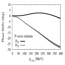
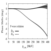
i.e. Wigner symmetry is fulfilled for even-L states while Serber symmetry holds for odd-L triplet states at distances above in agreement with the expectations spelled out at the beginning of this section. The parallel statements for phase shifts have been developed in detail in Ref. Calle Cordon and Ruiz Arriola (2008a) (see Fig. 3) where the relation of long distance symmetry and renormalization has been stressed. The remarkable aspect, already discussed there, is that the symmetry pattern while incompatible with Wigner symmetry for odd-L states is fully compatible with large expectations Kaplan and Manohar (1997). It does not explain, however, why Serber symmetry is a good one.


III Searching the symmetry
Most modern potential models of the NN interaction include OPE as the dominant longest range contribution. However, they differ at short distances where many effects compete and even are written in quite different forms (energy dependent, momentum dependent, angular momentum dependent, etc.). These ambiguities are of course compatible with the inverse scattering problem and manifest mainly in the off-shell behaviour of the NN forces. The relevant issue within the present context and which we analyze below regards the range and form of current NN interactions from the view point of long distance symmetries. Any potential fitting the elastic scattering data must posses the symmetries displayed by the phase-shifts sum rules as we see in Fig. 3. However, it is not obvious that potentials display the symmetry explicitly.
III.1 One Pion Exchange
The OPE potential reads
| (16) |
While OPE complies to the Wigner symmetry it does not embody exactly the Serber symmetry. Actually we get for even-L waves
| (17) | |||||
| (18) |
while for odd-L waves we have
| (19) | |||||
| (20) |
The factor for the singlet to triplet ratio is nonetheless a close approximation to the Serber limit in a region where the potential is anyhow small. These OPE relations are verified in practice for distances above . As we see from Fig. 2 the vanishing of potential happens down to the region around . For lower distances, potential models start deviating from each other (see e.g. Stoks et al. (1994)) but this vanishing of potential is a common feature which occurs beyond the validity of OPE.
III.2 Boundary conditions (alias )
We now analyze the symmetry issue for the highly successful PWA Stoks et al. (1993) of the Nijmegen group. There, a OPE potential is used down to and the interaction below that distance is represented by a boundary condition determined by a square well potential with an energy dependent height,
| (21) |
where stands for the corresponding channel, so that the total potential reads
where is a phenomenological intermediate range potential which acts in the region . Then, for the center of the L-multiplets ( V in MeV and k in fm ) we have
| (23) | |||||
| (24) | |||||
| (25) | |||||
| (26) |
where, again, we see that Serber symmetry takes place since and . Actually, the factor is strikingly similar to the of the OPE interaction which in the analysis of holds up to . Thus, in the Nijmegen PWA decomposition of the interaction we find the remarkable relation
| (27) |
showing that there is Serber symmetry in the short range piece of the potential. On the other hand, the even partial waves yield
| (28) | |||||
| (29) | |||||
| (30) | |||||
| (31) | |||||
| (32) | |||||
| (33) |
where we clearly see the violations of Wigner symmetry at short distances, i.e. we only have
| (34) |
This simple analysis suggests that Serber symmetry, when it works, holds to shorter distances than the Wigner symmetry. Our previous analysis in terms of mean phases Calle Cordon and Ruiz Arriola (2008a) fully supports this fact. Indeed, higher partial waves with angular momentum are necessarily small at small momenta due to the well known threshold behaviour. In fact, this is the case for and . However, Serber symmetry implies that and are rather small not only in the threshold region but also in the entire elastic region as can be clearly seen from Fig. 3.
III.3 Potentials and
A somewhat different perspective arises from a Wilsonian analysis of the NN interaction which corresponds to a coarse graining of the potential. This viewpoint was implemented in Ref. Bogner et al. (2003) where the so-called approach has been pursued, and corresponds to integrating out high momentum modes below a given cut-off from the Lippmann-Schwinger equation. It was found that high quality potential models, i.e. fitting the NN data to high accuracy and also incorporating OPE, collapse into a unique self-adjoint nonlocal potential for . This is a not a unreasonable result since all the potentials provide a rather satisfactory description of elastic NN scattering data up to . Moreover, the potential which comes out from eliminating high energy modes can be accurately represented as the sum of the truncated original potential and a polynomial in the momentum Holt et al. (2004),
| (35) |
where is the original potential in momentum space for a given partial wave channel and is the effect of the high energy states,
| (36) |
where the coefficients play the role of counterterms. It should be noted that here is cut-off independent whereas does depend on . When the potential given by Eq. (35) is plugged into the truncated Lippmann-Schwinger equation, i.e. intermediate states , the phase shifts corresponding to the full original potential are reproduced. In Fig. 4 the corresponding diagonal mean potentials are plotted for the Argonne-V18 force Wiringa et al. (1995) 222We thank Scott K. Bogner for kindly providing the numbers of Ref. Holt et al. (2004).. As we see both Wigner and Serber symmetries are, again, vividly seen. The important observation here is that the separation assumed by Eq. (35) does not manifestly display the symmetry. Actually, a more convenient representation would be to separate off all polynomial dependence explicitly from the original potential
| (37) |
so that if contains up to then starts off at , i.e. the next higher order. This way the departures from a pure polynomial may be viewed as true and explicit effects due to the potential. In terms of these polynomials, Wigner and Serber symmetries are formulated from the coefficients
| (38) |
constructed from the sum of the potential and the integrated out contribution below a cut-off , namely
| (39) |
It should be noted that the approach is in spirit nothing but the momentum space version of the PWA of the Nijmegen group in coordinate space where short distances, , are integrated out and parameterized by means of an energy dependent boundary condition. From this viewpoint the similarities as regards the Wigner and Serber symmetries are not surprising. This is why the standard boundary condition approach might be also denominated (see also Ref. Entem et al. (2007) for further discussions).


III.4 Chiral two pion exchange
The chiral Two Pion Exchange (TPE) potentials computed in Ref. Kaiser et al. (1998) are understood as direct consequences of the spontaneous chiral symmetry breaking in QCD. Actually, the TPE contribution takes over the OPE one at about . At very long distances one has
| (40) |
where and are the pion and nucleon masses respectively, the axial coupling constant and the pion weak decay constant. As we see Serber symmetry is broken already at long distances. Generally, these chiral potentials are supplemented by counterterms or equivalently boundary conditions when discussing NN scattering and generating phase shifts (see e.g. Ref. Rentmeester et al. (1999)). Given that these NN phase shifts do fulfill the symmetry (see Fig. 3) we expect that the breaking of the symmetry at long distances must be compensated by the counterterms which encode the unknown short distance physics Rentmeester et al. (1999). This can be verified by looking e.g. at the potential corresponding to the Next-to-next-to-next-to-leading order (N3LO) chiral potential which contains its own cut-off parameter of Entem and Machleidt (2003). This potential contains OPE and describes successfully the data and hence falls into the universality class of high-quality potentials Bogner et al. (2007) when the common cut-off scale is used. If the chiral potential is slightly detuned by taking one sees a low momentum violation of the Wigner symmetry in Fig. 5 in total contradiction with the fact that one expects that asymptotically OPE should dominate. This shows that regarding the symmetry is fine-tuned. A more complete account of these issues will be presented elsewhere Pavon Valderrama and Ruiz Arriola (2009).


IV Are counterterms fingerprints of long distance symmetries ?
Given the fact that both Wigner and Serber symmetries can be interpreted as long distance symmetries which roughly materialize at low energies in the potentials (see Fig. 2), the phase shifts (see Fig. 3) and the potentials (see Fig. 4) we find it appropriate to discuss how these results fit into renormalization ideas and the role played by the corresponding counterterms.
IV.1 The perturbative point of view
As we have mentioned in the previous section, chiral potentials are generally used to describe NN scattering with the additional implementation of counterterms which cannot directly be determined from chiral symmetry alone. On the other hand, one expects these counterterms to encode short distance physics and hence to be related to the exchange of heavier mesonic degrees of freedom alike those employed in the One Boson Exchange (OBE) potentials Machleidt et al. (1987). The idea is quite naturally based on the resonance saturation hypothesis of the exchange forces (see e.g. Ecker et al. (1989) for a discussion in the scattering case). This is achieved by integrating out the heavy fields using their classical equations of motion, and expanding the exchanged momentum between the nucleons as compared to the resonance mass case Epelbaum et al. (2002, 2004). Schematically it corresponds to power expand the Yukawa-like NN potentials (we ignore spin and isospin for simplicity),
| (41) | |||||
where we are working in the CM system and we take the momentum transfer as . The meaning of the terms above is as follows: is an s-wave zero range, is an s-wave finite range, is a p-wave etc. . More generally, Eq. (41) corresponds to a power series expansion of the potential in momentum space. Obviously, we expect such a procedure to be meaningful whenever the scattering process can be treated perturbatively, like e.g. the case of peripheral waves. As is well known, central s-waves cannot be treated perturbatively as the corresponding scattering amplitudes have poles very close to threshold corresponding a virtual state in the channel and the deuteron in the channel. This does not mean, however, that the potential cannot be represented in the polynomial form of Eq. (41), but rather that the coefficients cannot be computed directly as the Fourier components of the potential.
IV.2 The Wilsonian point of view
The momentum space approach Holt et al. (2004) makes clear that the long distance behaviour of the theory is not determined by the low momentum components of the original potential only, one has to add virtual high energy states which also contribute to the interaction at low energies in the form of counterterms, as outlined by Eqs. (35) and (37). Alternatively the more conventional coordinate space boundary condition (alias ) method shows that the low energy behaviour of the theory is not determined only by the long distance behaviour of the potential, one has to include the contribution from integrated out short distances in the form of boundary conditions. A true statement is that the low momentum features of the interaction in the potential can be mapped into long distance characteristics of the potential . The symmetries are formulated in terms of the conditions in Eq. (39).
IV.3 Long distance symmetries in Nuclear Potentials
In order to substantiate our points further, let us note that in Ref. Holt et al. (2004) it was suggested that the was a viable way of determining the effective interactions which could be further used in shell model calculations for finite nuclei. Actually, this interpretation when combined with our observation of Fig. 4 that Serber symmetry shows up quite universally has interesting consequences. Schematically, this can be implemented as a Skyrme type effective (pseudo)potential Skyrme (1959)
| (42) | |||||
where is the spin exchange operator with for spin single and for spin triplet states. The dots stand for spin-orbit, tensor interaction, etc. It should be noted the close resemblance of the momentum space version of this potential
| (43) | |||||
with Eq. (37) after projection onto partial waves, where only S- and P-waves have been retained. Traditionally, binding energies have been used to determine the parameters and within a mean field approach and many possible fits arise depending on the chosen observables (see e.g. Ref. Chabanat et al. (1997)) possibly displaying some spurious short distance sensitivity beyond the range of applicability of Eq. (42). The low momentum character of the Skyrme force, suggests using the longest possible wavelength properties. Actually, inclusion of tensor force and a new fitting strategy to single particle energies Zalewski et al. (2008) yields which is an almost perfect Serber force for spin-triplets () and reproduces the so-called SLy4 form of the Skyrme functional Chabanat et al. (1997). On the light of our discussion this result seems quite natural as single particle energies place attention in long wavelength states, a situation where can be described by a pure polynomial in momentum (see Eq. (37)) and Serber symmetry becomes manifest directly from a coarse graining of the NN-interaction.
IV.4 Matching OBE potentials to chiral potentials
In Ref. Epelbaum et al. (2002) a systematic determination of counterterms has been carried out for a variety of realistic potentials which successfully fit the NN data by reading off the Fourier components of the potential (see e.g. Eq. (41)). The counterterms so obtained are then compared to those determined from direct fits to the NN data when the chiral potential is added. The spread of values for these counterterms found in Ref. Epelbaum et al. (2002) for realistic potentials, however, does not comply to the fact that all those potentials provide a quite satisfactory description of the phase shifts. Moreover, in Ref. Epelbaum et al. (2002) it is found that for the OBE Bonn potential Machleidt et al. (1987)
| (44) | |||||
| (45) | |||||
Thus, the triplet to singlet ratio is in this case. For the CD Bonn potential Machleidt (2001) one has whereas Argonne AV-18 Wiringa et al. (1995) yields . These large factors contrast with the much smaller factor of the PWA sketched above in Sect. III.2. They also disagree with the almost vanishing ratio found for the potentials described in Section III.3 which yield a universal result (see also Fig. 4 for the particular AV-18 potential). The reason is that the correct formulation of the symmetry conditions is given by Eq. (39) which are made up from the potential plus the contribution of the high energy tail. Thus, it appears that in the approach of Ref. Epelbaum et al. (2002) Serber symmetry is more strongly violated at short distances than expected from other means. In our view the spread of values found in Ref. Epelbaum et al. (2002) might possibly reflect an inadequacy of the method used to characterize the long distance coarse grained NN dynamics where, as we have shown, Serber symmetry becomes quite accurate. Actually, the matching of counterterms between, say, the OBE potential and the chiral potentials is done in terms of objects which have a radically different large behaviour (see Section V for further details). For instance, while because and one has since , and . In fact, the value of the counterterms determined from resonance exchange is generally not simply determined by the coefficients of the power series expansion of potential in momentum space, as schematically given by Eq. (41), since they undergo renormalization and hence run with the scale.
IV.5 Long distance symmetry and off-shellness
The previous analysis shows that nothing forbids to have a potential which breaks the symmetry strongly on the one hand and being able to simultaneously fit the scattering data which manifestly display the symmetry on the other hand. Actually, this can only be achieved by some degree of compensating symmetry violation between long and short distances 333This is the case for instance of chiral TPE potentials, see Section III.4, where the potential Kaiser et al. (1998) breaks the symmetry above but the data can be described Rentmeester et al. (1999) with this truncated potential plus suitable energy dependent boundary conditions.. However, it is somewhat unnatural as it does not reflect the true character of the theory and relegates the role of the symmetry to be an accidental one. As it is widely accepted, unveiling symmetries is not mandatory but makes life much easier 444The above discussion is somewhat similar to the use of regularization schemes in EFT; while it is possible to break the symmetry by all allowed counterterms, final physical results will depend on redundant combinations of parameters expressing the symmetry. In practice it is far more convenient to use a regularization scheme where the symmetry is preserved manifestly..
Of course, these observations are true as long as we restrict to on-shell properties, such as NN scattering. However, would these symmetries have any consequence for off-shell nucleons ?. One may clearly have arbitrary short distance parameterizations of the force without a sizeable change of the phase shifts. However, the universality of long distance potentials above or, equivalently, a coarse graining of the interaction with the given length scale such as is by definition based on insensitivity to shorter wavelengths. Our discussion above on effective forces illustrates the fact that these redefinitions of the potential in the NN scattering problem cannot affect the effective force and so a violation of the Serber symmetry has a physical significance for wavelengths larger than the coarse graining scale.
V Serber force from a large perspective
Up till now, in this paper we have provided evidence that long distance symmetries such as Wigner’s and Serber’s do really take place in the two nucleon system. From now on we are concerned with trying to determine whether those symmetries are purely accidental ones or obey some pattern following more closely from QCD. Actually, we found Calle Cordon and Ruiz Arriola (2008a) that large limit ’t Hooft (1974); Witten (1979) (for comprehensive reviews see e.g. Manohar (1998); Jenkins (1998); Lebed (1999)) provides a rationale for Wigner symmetry. The fact that Serber symmetry holds when Wigner symmetry fails suggests analyzing the large consequences more thoroughly. While we do not find a completely unique answer regarding the origin of Serber symmetry, the analysis does show interesting features, as will be discussed.
V.1 The large expansion
In this section we want to analyze these long distance Serber and Wigner symmetries within the two nucleon system from the large expansion ’t Hooft (1974); Witten (1979) (for comprehensive reviews see e.g. Manohar (1998); Jenkins (1998); Lebed (1999)). One feature of large which becomes relevant for the NN problem is that is does not specially hold for long or short distances. This allows in particular to switch from perturbative quarks and gluons at short distances to the non-perturbative hadrons, the degrees of freedom of interest to nuclear physics. This quark-hadron duality makes possible the applicability of large counting rules directly to baryon-meson interactions, at distances where explicit quark-gluon effects are not expected to be crucial. The procedure provides utterly a set of consistency conditions from which the contracted SU(4) symmetry is deduced Manohar (1998); Jenkins (1998); Lebed (1999). Thus, while the large scaling behaviour and spin-flavour structure of the NN potential, Eq. (46), is directly established in terms of quarks and gluons Kaplan and Manohar (1997), quark-hadron duality at distances larger than the confinement scale requires an identification of the corresponding exchanged mesons, and hence a link to the OBE potentials is provided. However, for internal consistency of the hadronic version of the large expansion, these counting rules should hold regardless of the number of exchanged mesons between the nucleons. Actually, naive power counting suggests huge violations of the NN counting rules. The issue has been clarified after the work of Banerjee, Cohen and Gelman for all meson exchange cases with spin 0 and spin 1 Banerjee et al. (2002) where the necessary cancellations between meson retardation in direct box diagrams and crossed box diagrams was indeed shown to take place. In the TPE case the -isobar embodying the contracted SU(4) symmetry was explicitly needed. Although the exchange of three and higher mesons appeared initially to present puzzling inconsistencies Belitsky and Cohen (2002) a possible outcome was outlined in Ref. Cohen (2002) by noting that large counting rules apply to energy independent and hence self-adjoint potentials.
V.2 Large potentials
Based on the contracted SU(4) large symmetry the spin-flavour structure of the NN interaction was analyzed by Kaplan, Savage and Manohar Kaplan and Savage (1996); Kaplan and Manohar (1997) who found that the leading nucleon-nucleon potential indeed scales as and has the structure
| (46) |
It is noteworthy that the tensor force appears at the leading order in the large expansion. From the large potential, Eq. (46), we have for the center of multiplet potentials the sum rules
where as we see for odd-L. Thus, large implies Wigner symmetry in even-L channels and allows a violation of Wigner symmetry in odd-L partial waves while it allows a violation of Serber symmetry in spin singlet channels. The question is whether or not large implies Serber symmetry in spin triplet channels as we observe both for the potentials in Fig. 2 as well as for the phase shifts in Fig. 2. On the other hand, from the odd-waves we see from Fig. 3 that the mean triplet phase is close to null, thus one might attribute this feature to an accidental symmetry where the odd-waves potentials are likewise negligible. In the large limit this means , a fact which should be verified.
V.3 OBE large potentials
According to Refs. Kaplan and Savage (1996); Kaplan and Manohar (1997) in the leading large one has while . To proceed further and gain some insight we write the potentials in terms of leading single meson exchanges (see also Ref. Banerjee et al. (2002)) one has Yukawa like potentials (we use the notation of Ref. Machleidt et al. (1987))
where is a scale which is numerically equal to the nucleon mass and is . All meson couplings scale as whereas all meson masses scale as . In principle there would be infinitely many contributions but we stop at the vector mesons. A relevant question which will be postponed to the next Section regards what values of Yukawa masses should one take. This is particularly relevant for the case. Note that the tensorial structure of the potential Eq. (46) is complete to . This leaves room for corrections to the NN potential without generating new dependences triggered by sub-leading mass shifts and sub-leading vertex corrections .
As we have mentioned above, to obtain Serber symmetry we must get a large cancellation. At short distances the Yukawa OBE potentials have Coulomb like behavior with the dimensionless combinations
where the small OPE contribution has been dropped. To resemble Serber symmetry we should have . There are several scenarios where this can be achieved. For instance, if we impose the OPE 1/9-rule for the full potential we have . Using SU(3), , Sakurai’s universality , the current-algebra KSFR relation, , and the scalar Goldberger-Treiman relation, , one would get a not unreasonable result. This only addresses the cancellation at short distances. The cancellation would be more effective at intermediate distances if and would be numerically closer. In this regard, let us note that there are various schemes where an identity between scalar and vector meson masses are explicitly verified Weinberg (1990); Svec (1997); Megias et al. (2004). In reality, however, the scalar and vector masses are sufficiently different vs . In the next Section we want to analyze this apparent contradiction.
VI From resonances to Yukawa potentials
VI.1 Correlated two pion exchange
As we have already mentioned TPE is a genuine test of chiral symmetry. On the other hand, it is well known that the iterated exchange of two pions may become in the -channel either a or a resonance for isoscalar and isovector states respectively. While the interactions leading to this collectiveness are controlled to a great extent by chiral symmetry Oller et al. (1998); Nieves and Ruiz Arriola (2000); Nieves et al. (2002), the resulting contributions to the NN potential in terms of boson exchanges bear a very indirect relation to it. The relation of the ubiquitous scalar meson in nuclear physics and NN forces in terms of correlated two pion exchange has been pointed out many times Partovi and Lomon (1970); Machleidt et al. (1987); Lin and Serot (1990); Kim et al. (1994) (see e.g. Refs. Kaiser et al. (1998); Oset et al. (2000); Kaskulov and Clement (2004); Donoghue (2006) for a discussion in a chiral context). Attempts to introduce chiral Lagrangeans in nuclear physics have been numerous Stoks and Rijken (1997); Furnstahl et al. (1997); Papazoglou et al. (1999) but the implications for the OBE potential are meager despite the fact that useful relations among couplings can be deduced 555We should mention the Goldberger-Treimann relation for pions and scalars which yields and and the KSFR-universality relation which yields . As we will see, they are complementary information to the large requirements.
Note that the leading term generating the scalar meson is but occurs first at N3LO in the chiral counting. The central potential reads Kaiser et al. (1998); Oset et al. (2000); Kaskulov and Clement (2004); Donoghue (2006),
| (52) |
where is the sigma term and the scattering amplitude in the channel as a function of the CM energy (see also Eq. (54)). Under the inclusion of resonance contributions Eq. (52) is modified by an aditive redefinition of to include those -states Oset et al. (2000). In the large limit, while yielding as expected Kaplan and Manohar (1997). Actually, at the sigma pole
| (53) | |||||
where in the second step we have taken the large limit. This yields , provided and . The “fictitious” narrow exchange has been attributed to intermediate states Kaiser et al. (1998), to iterated pions Donoghue (2006) or both Oset et al. (2000). This identification is based on fitting the resulting r-space potentials to a Yukawa function in a reasonable distance range.
VI.2 Exchange of Pole Resonances
In this section we separate the resonance contribution to the potential from the background, neglecting for simplicity the vertex correction in Eq. (52). The most obvious definition of the or propagator is via the scattering amplitude in the scalar-isoscalar and vector-isovector channels, and respectively. Using the definition
| (54) |
with the phase space in our notation. Taking into account the fact that on the second Riemann sheet (taking as an example) the amplitude has a pole
| (55) |
with the pole position and the corresponding residue. Here we define, as usual, the analytical continuation as
| (56) |
By continuity and thus unitarity requires . One has for the (suitably normalized) scalar propagator
| (57) |
in the whole complex plane. In particular
| (58) |
where the phase is defined as and is related to the background, i.e. the non-pole contribution. In Appendix A we discuss a toy model for scattering Binstock and Bryan (1971) which proves quite useful to fix ideas. The function is analytic in the complex s-plane with a right cut along the line stemming from unitarity in scattering and a left cut running from due to particle exchange in the and channels. Assuming the scattering amplitude to be proportional to this propagator the corresponding phase shift is then given by
| (59) |
The propagator satisfies the unsubtracted dispersion relation Ericson and Weise (1988),
| (60) |
where the spectral function is related to the discontinuity across the unitarity branch cut 666Defined as for a real function below threshold, .
| (61) | |||||
| (62) |
which satisfies the normalization condition
| (63) |
where is the integrated strength. Thus, the Fourier transformation of the propagator is
| (64) | |||||
According to Eq. (63), for small distances. We define the analytic function for in the cut plane without and where
| (65) |

and fulfilling the boundary value condition . This function has a pole at the complex point and a square root branch cut at triggered by the phase space factor only since is continuous, so that . Thus, we can write the spectral integral, Eq. (64) as running below the unitarity cut and by suitably deforming the contour in the fourth quadrant in the second Riemann Sheet, as shown in Fig. 6, we can separate explicitly the contribution from the pole and the background yielding
| (66) |
While, in principle, both contributions are complex, the total result must be real and their imaginary parts cancel identically (see Appendix A for a specific example). Using that Eq. (56) implies the -pole contribution is effectively given by
which is an oscillating function damped by an exponential. In the narrow resonance limit, , one has yielding
| (68) |
which is a Yukawa potential. The background reads
| (69) | |||||
At large distances the integral is dominated by the small region, and we get the distinct TPE behaviour . The pre-factor is obtained by expanding at small and using that unitarity imposes the spectral density to be proportional to the phase space factor, Eq. (62). Close to threshold, , involves the scattering length defined as yielding
| (70) |
We therefore get
| (71) | |||||
In Appendix A the pole-background decomposition in Eq. (66) is checked explicitly in a toy model. The resonance contribution saturates the normalization completely, the continuum background yielding a vanishing contribution to the integrated strength. On the other hand, the resonance produces a Yukawa tail with an oscillatory modulation which alternates between attraction and repulsion, although the region where the oscillation is relevant depends largely on .
VI.3 resonances at large
The large analysis also opens up the possibility to a better understanding of the role played by the ubiquitous scalar meson. This is an essential ingredient accounting phenomenologically for the mid range nuclear attraction and which, with a mass of , was originally proposed in the fifties Johnson and Teller (1955) to provide saturation and binding in nuclei. Along the years, there has always been some arbitrariness on the “effective” or ”fictitious” scalar meson mass and coupling constant to the nucleon, partly stimulated by lack of other sources of information 777For instance, in the very successful Charge Dependent (CD) Bonn potential Machleidt (2001) any partial wave -channel is fitted with a different scalar meson mass and coupling.. During the last decade, the situation has steadily changed, and insistence and efforts of theoreticians Tornqvist and Roos (1996), have finally culminated with the inclusion of the resonance (commonly denoted by ) in the PDG Yao et al. (2006) as the seen as a resonance, with a wide spread of values ranging from for the mass and a for the width are displayed van Beveren et al. (2002). These uncertainties have recently been sharpened by a benchmark determination based on Roy equations and chiral symmetry Caprini et al. (2006) yielding the value . Once the formerly fictitious sigma has become a real and well determined lowest resonance of the QCD spectrum it is mandatory to analyze its consequences all over. Clearly, these numbers represent the value for , but large counting requires that for mesons and .
In this regard the large analysis may provide a clue of what value should be taken for the mass Calle Cordon and Ruiz Arriola (2008b) 888Large studies in scattering based on scaling and unitarization with the Inverse Amplitude Method (IAM) of ChPT amplitudes provide results which regarding the troublesome scalar meson depend on details of the scheme used. While the one loop coupled channel approach Pelaez (2004) yields any possible and a large width (in apparent contradiction with standard large counting ’t Hooft (1974); Witten (1979)), the (presumably more reliable) two loop approach Pelaez and Rios (2006), yields a large mass shift (a factor of 2) for the scalar meson when going from to yielding , but a small shift in the case of the meson. One should note the large uncertainties of the two loop IAM method documented in Ref. Nieves et al. (2002). Based on the Bethe-Salpeter approach to lowest order Nieves and Ruiz Arriola (2000) we have estimated Calle Cordon and Ruiz Arriola (2008b).. Of course, similar remarks apply to the width of other mesons, such as , as well. If we make use of the large expansion according to the standard assumption ()
| (72) | |||||
| (73) |
the pole contribution becomes
| (74) |
where , representing the resonance mass to NLO in the expansion, should be used. Note that the width does not contribute to this order. Thus, for all purposes we may use a Yukawa potential to represent the exchange of a resonance. However, what is the numerical value of this one should use for the NN problem?. Model calculations based on scaling of chiral unitary phase shifts for suggest sizeable modifications as compared with the accurately determined pole position when is varied but the numerical results are not very robust Nieves and Ruiz Arriola (2009) 999Actually, according to Ref. Flambaum and Shuryak (2007) the effect of a meson width in the Yukawa-like potential is which corresponds to a NLO large renormalization of the mass and coupling and providing a correction to the central potential. The analysis is based on separating the integrand into different intervals which become dominant at large distances. Our analysis separates first the pole contribution form the background and then studies each contribution separately. We note however, that one can extract a Yukawa potential of the meson even for the large and physical width in the region where the potential is operating with quite sensible values Binstock and Bryan (1971). In Appendix B we update this analysis using recent parameterizations of scattering provided in Refs. Yndurain et al. (2007); Caprini (2008) confirming the Yukawa behaviour. The main reason is that the the potential is being probed for space-like exchanged four momentum, while the resonance behaviour takes place in the time-like region corresponding to the crossed process .. An alternative viewpoint where, to the same accuracy, the large -NLO pole contribution could be replaced by the equivalent Breit-Wigner resonance mass to the same approximation, since according to Nieves and Ruiz Arriola (2009) we may take
| (75) |
Thus, at LO and NLO in the large limit the exchange of a resonance between nucleons can be represented at long distances as a Yukawa potential with the Breit-Wigner mass to . The vertex correction , see e.g. Eq. (52), just adds a coupling constant yielding
| (76) |
Of course, the same type of arguments apply to the -meson exchange, with the only modification
| (77) |
where now . In Fig. 7 we show the data for phase shifts, where we see that the true Breit-Wigner masses or not very different. Of course, these arguments do not imply that the Yukawa masses should exactly coincide, but at least suggest that one should expect a large shift for the mass from the pole position and a very small one for the meson mass when the next-to-leading correction to the pole masses are considered. The identity of scalar and vector masses has been deduced from several scenarios based on algebraic chiral symmetry Weinberg (1969, 1990). Actually, it has been shown that without appealing to the strict large limit but assuming the narrow resonance approximation (See also Ref. Weinberg (1994)).


VII conclusions
Serber symmetry seems to be an evident but puzzling symmetry of the NN system. Since it was proposed more than 70 years ago no clear explanation based on the more fundamental QCD Lagrangean has been put forward.
In the present paper we have analyzed the problem from the viewpoint of long distance symmetries, a concept which has proven useful in the study of Wigner spin-flavour symmetry. Actually, Serber symmetry is clearly seen in the np differential cross section implying a set of sum rules for the partial wave phase shifts which are well verified to a few percent level in the entire elastic region. While this situation corresponds to scattering of on-shell nucleons, it would be rather interesting to establish the symmetry beyond this case. Therefore, we have formulated these sum rules at the level of high quality potentials, i.e. potentials which describe elastic NN scattering with which are also well verified at distances above . This suggests that a coarse graining of the NN interaction might also display the symmetry. The equivalent momentum space Wilsonian viewpoint is implemented explicitly by the approach by integrating all modes below a certain cut-off . By analyzing existing calculations for high quality potentials we have shown that Serber symmetry is indeed fulfilled to a high degree. We remind that within the approach this symmetry has direct implications in shell model calculations for finite nuclei since the potential corresponds to the effective nuclear interaction.
A surprising finding of the present paper is that chiral potentials, while implementing extremely important QCD features, do not fulfill the symmetry to the same degree as current high quality potentials. This effect must necessarily be compensated by similar symmetry violations in the counterterms encoding the non-chiral and unknown short distance interaction and needed to describe NN phase shifts where the symmetry does indeed happen. While this is not necessarily a deficiency of the chiral approach it is disturbing that the symmetry does not manifest at long distances, unlike high quality potentials. This may be a general feature of chiral potentials which requires further investigation Pavon Valderrama and Ruiz Arriola (2009).
In an attempt to provide a more fundamental understanding of the striking but so far accidental Serber symmetry, we have also speculated how it might arise from QCD within the large perspective on the second part of the paper. The justification for advocating such a possible playground is threefold. Firstly, the NN potential tensorial structure is determined with a relative accuracy, which naively suggests a bold . In the second place, the meson exchange picture is justified. Finally, we have found previously that such an expansion provides a rationale for the equally accidental and pre-QCD Wigner symmetry. Actually, we found that large predicts the NN channels where Wigner symmetry indeed works and fails phenomenologically. The intriguing point is that when Wigner symmetry fails, as allowed by large considerations, Serber symmetry holds instead. In the present paper we have verified the previous statements at the level of potentials at large distances or using potentials, reinforcing our previous conclusions based on just a pure phase shift analysis. Under those circumstances, it is therefore natural to analyze to what extent and even if Serber symmetry could be justified at all from a large viewpoint. In practical terms we have shown that within a One Boson Exchange framework, the fulfillment of the symmetry at the potential level is closely related to having not too dissimilar values of and meson masses as they appear in Yukawa potentials. Actually, these and states are associated to resonances which are seen in scattering and can be uniquely defined as poles in the second Riemann sheet of the scattering amplitude at the invariant mass . We have therefore analyzed the meaning of those resonances within the large picture, by assuming the standard mass and width scaling. We have found that, provided we keep terms in the potential to NLO, meson widths do not contribute to the NN potential, as they are , i.e. a relative correction to the LO contribution. This justifies using a Yukawa potential where the mass corresponds to an approximation to the pole mass which cannot be distinguished from the Breit-Wigner mass up to . This suggests that the masses and which appear in the OBE potential could be interpreted as an approximation to the pole mass rather than its exact value. This supports the customary two-Yukawa representation of complex-pole resonances pursued in phenomenological approaches since it was first proposed Binstock and Bryan (1971), since in practice only the lowest Yukawa mass contributes significantly. The question on what numerical value should be used for the Yukawa mass is a difficult one, and at present we know of no other direct way than NN scattering fits for which might be acceptable Calle Cordón and Ruiz Arriola (2009) when the uncorrelated contribution is disregarded.
On a more fundamental level, however, lattice QCD calculations at variable values (see e.g. Ref. Teper (2008) for a review) might reliably determine the Yukawa mass parameters appearing in the large potential. A recent quenched QCD lattice calculation yields Bali and Bursa (2008) with the string tension, which for yields for (see also Ref. Del Debbio et al. (2008)). The extension of those calculations to compute the needed mass shift would be most welcome and would require full dynamical quarks. Of course, one should not forget that Serber symmetry holds to great accuracy in the real world, and in this sense it represents a stringent test to lattice QCD calculations in -waves. Amazingly, the only existing of S-wave potential calculationIshii et al. (2007) displays Wigner symmetry quite accurately.
In any case the large form of the potential Eq. (46) can be retained with relative accuracy since meson widths enter beyond that accuracy as sub-leading corrections, on equal footing with many other effects (spin-orbit, relativistic and other mesons), independently on how large the width is in the real world. In our view this paves the way for further investigations on the relevance of large based ideas for the two nucleon system.
Acknowledgements.
We gratefully acknowledge Manuel Pavón Valderrama for a critical reading of the manuscript, Juan Nieves, Lorenzo Luis Salcedo and José Ramón Peláez for discussions and Scott K. Bogner for kindly providing the data corresponding to the V18 potentials of Ref. Bogner et al. (2003). We also thank Jacek Dobaczewski and Rupp Machleidt for useful communications. This work has been partially supported by the Spanish DGI and FEDER funds with grant FIS2008-01143/FIS, Junta de Andalucía grant FQM225-05, and EU Integrated Infrastructure Initiative Hadron Physics Project contract RII3-CT-2004-506078.Appendix A Toy model for scattering
In this appendix we illustrate with a specific example our discussion of Section VI and in particular the pole-background decomposition of Eq. (66). According to Ref. Binstock and Bryan (1971) the finite width of the scalar meson can be modelled by the propagator
| (78) |
for . Below the elastic scattering threshold we use the standard definition where . This defines the propagator in the first Riemann sheet, the second Riemann sheet is determined from the usual continuity equation . The pole position is given by
| (79) | |||||
In the small width limit the position of the pole and width are
| (80) | |||||
| (81) |
Despite the large -width this expansion works because the -factor yields (the next correction has a numerical , see below). Assuming the scattering amplitude to be proportional to this propagator the corresponding phase shift is then given by
| (82) |
The parameterization is such that the standard Breit-Wigner definition of the resonance is fulfilled for the bare parameters,
| (83) |
Of course, in the limit of narrow resonances both definitions are indistinguishable and we have and . If we use the pole position in the second Riemann sheet of the S-matrix or equivalently the zero in the first Riemann sheet from Caprini et al. (2006) yielding the value we get
| (84) |
From the small width expansion, Eq. (81), one gets , despite the apparent large width. From Ref. Leutwyler (2008) one has the magnitude of the residue whereas we get . Note the shift between the Breit-Wigner and the pole position. With the above parameters the scattering length is which is clearly off the value deduced from ChPT. The propagator satisfies the unsubtracted dispersion in Eq. (60) where the spectral function is given by
and satisfies the normalization condition given by Eq. (63) with . Thus, using the Fourier transformation of the propagator and separating explicitly the contribution from the poles and the background in Eq. (66). This yields the result depicted in Fig. (8) which illustrates and checks the pole-background decomposition and shows that the total contribution, although describable by a Yukawa shape does not correspond to the pole piece. In addition the cancellation of imaginary parts, , is explicitly verified.


Using the inverse relations of Eq. (81), in the narrow width approximation the pole contribution becomes
in qualitative agreement with Eq. (68). On the other hand the contribution at long distances becomes
| (87) | |||||
The asymptotic form in the first lime reproduces accuracy the full result Eq. (66) for .
Finally, the meson propagator and the associated phase shift can be dealt with mutatis mutandis by using
| (88) |
where the wave character of the decay can be recognized in the phase space factor.
Appendix B Realistic scalar-isoscalar scattering
Realistic parameterizations of the scattering data have been proposed based on the conformal mappings Yndurain et al. (2007); Caprini (2008) with several variations. Our results show little dependence on those and we show here the ghost-full version and the Adler zero located at the lowest order ChPT Yndurain et al. (2007) which reads
| (89) |
where the conformal mapping is
| (90) |
For the three sets of parameters discussed in Ref. Yndurain et al. (2007) the resulting complex pole position is slightly higher than the Roy equation value Caprini et al. (2006). If we use the dispersive representation for given in Eq. (64) and cut the integral at the threshold we get a function which can be fitted in the range by a Yukawa potential with . The uncertainty corresponds to changing the parameters within errors Yndurain et al. (2007) as well as the varying the fitting interval. This is the modern version of the result found long ago Binstock and Bryan (1971) using a relativistic Breit-Wigner form (see Appendix A).
References
- Epelbaum et al. (2008) E. Epelbaum, H.-W. Hammer, and U.-G. Meißner (2008), eprint 0811.1338.
- Serber (1938) R. Serber, Phys. Rev. 53, 211 (1938).
- Ashkin and Wu (1948) J. Ashkin and T.-Y. Wu, Phys. Rev. 73, 973 (1948).
- Christian (1952) R. S. Christian, Reports on Progress in Physics 15, 68 (1952).
- Blatt and Weisskopf (1952) J. Blatt and V. Weisskopf, Theoretical Nuclear Physics (John Wiley & Sons, 1952).
- Christian and Hart (1950) R. S. Christian and E. W. Hart, Phys. Rev. 77, 441 (1950).
- Gerjuoy (1950) E. Gerjuoy, Phys. Rev. 77, 568 (1950).
- Nakabayasi and Sato (1952) K. Nakabayasi and I. Sato, Phys. Rev. 88, 144 (1952).
- Jastrow (1951) R. Jastrow, Phys. Rev. 81, 165 (1951).
- Hull et al. (1961) M. H. Hull, K. E. Lassila, H. M. Ruppel, F. A. McDonald, and G. Breit, Phys. Rev. 122, 1606 (1961).
- de la Ripelle et al. (2005) M. F. de la Ripelle, S. A. Sofianos, and R. M. Adam, Ann. Phys. 316, 107 (2005), eprint nucl-th/0410016.
- Fetter and Walecka (1971) A. Fetter and J. Walecka, Quantum Theory of Many-Panicle Systems (McGraw–Hill, New York, 1971).
- Bethe and Longmire (1950) H. A. Bethe and C. Longmire, Phys. Rev. 77, 647 (1950).
- Lashko and Filippov (2007) Y. A. Lashko and G. F. Filippov, Physics of Atomic Nuclei 70, 1440 (2007).
- Ali et al. (1985) S. Ali, A. A. Z. Ahmad, and N. Ferdous, Rev. Mod. Phys. 57, 923 (1985).
- Skyrme (1959) T. Skyrme, Nucl. Phys. 9, 615 (1959).
- Chabanat et al. (1997) E. Chabanat, J. Meyer, P. Bonche, R. Schaeffer, and P. Haensel, Nucl. Phys. A627, 710 (1997).
- Zalewski et al. (2008) M. Zalewski, J. Dobaczewski, W. Satula, and T. R. Werner, Phys. Rev. C77, 024316 (2008), eprint 0801.0924.
- Stoks et al. (1993) V. G. J. Stoks, R. A. M. Kompl, M. C. M. Rentmeester, and J. J. de Swart, Phys. Rev. C48, 792 (1993).
- Stoks et al. (1994) V. G. J. Stoks, R. A. M. Klomp, C. P. F. Terheggen, and J. J. de Swart, Phys. Rev. C49, 2950 (1994), eprint nucl-th/9406039.
- Ishii et al. (2007) N. Ishii, S. Aoki, and T. Hatsuda, Phys. Rev. Lett. 99, 022001 (2007), eprint nucl-th/0611096.
- Beane et al. (2006) S. R. Beane, P. F. Bedaque, K. Orginos, and M. J. Savage, Phys. Rev. Lett. 97, 012001 (2006), eprint hep-lat/0602010.
- Calle Cordon and Ruiz Arriola (2008a) A. Calle Cordon and E. Ruiz Arriola, Phys. Rev. C78, 054002 (2008a), eprint 0807.2918.
- Wigner (1937) E. Wigner, Phys. Rev. 51, 106 (1937).
- Hund (1937) F. Hund, Zeitschrift fur Physik 105, 202 (1937).
- ’t Hooft (1974) G. ’t Hooft, Nucl. Phys. B72, 461 (1974).
- Witten (1979) E. Witten, Nucl. Phys. B160, 57 (1979).
- Manohar (1998) A. V. Manohar (1998), eprint hep-ph/9802419.
- Jenkins (1998) E. E. Jenkins, Ann. Rev. Nucl. Part. Sci. 48, 81 (1998), eprint hep-ph/9803349.
- Lebed (1999) R. F. Lebed, Czech. J. Phys. 49, 1273 (1999), eprint nucl-th/9810080.
- Kaplan and Savage (1996) D. B. Kaplan and M. J. Savage, Phys. Lett. B365, 244 (1996), eprint hep-ph/9509371.
- Kaplan and Manohar (1997) D. B. Kaplan and A. V. Manohar, Phys. Rev. C56, 76 (1997), eprint nucl-th/9612021.
- Banerjee et al. (2002) M. K. Banerjee, T. D. Cohen, and B. A. Gelman, Phys. Rev. C65, 034011 (2002), eprint hep-ph/0109274.
- Caprini et al. (2006) I. Caprini, G. Colangelo, and H. Leutwyler, Phys. Rev. Lett. 96, 132001 (2006), eprint hep-ph/0512364.
- Amsler et al. (2008) C. Amsler et al. (Particle Data Group), Phys. Lett. B667, 1 (2008).
- Wiringa et al. (1995) R. B. Wiringa, V. G. J. Stoks, and R. Schiavilla, Phys. Rev. C51, 38 (1995), eprint nucl-th/9408016.
- Bogner et al. (2003) S. K. Bogner, T. T. S. Kuo, and A. Schwenk, Phys. Rept. 386, 1 (2003), eprint nucl-th/0305035.
- Holt et al. (2004) J. D. Holt, T. T. S. Kuo, G. E. Brown, and S. K. Bogner, Nucl. Phys. A733, 153 (2004), eprint nucl-th/0308036.
- Entem et al. (2007) D. R. Entem, E. Ruiz Arriola, M. Pavon Valderrama, and R. Machleidt (2007), eprint 0709.2770.
- Kaiser et al. (1998) N. Kaiser, S. Gerstendorfer, and W. Weise, Nucl. Phys. A637, 395 (1998), eprint nucl-th/9802071.
- Rentmeester et al. (1999) M. C. M. Rentmeester, R. G. E. Timmermans, J. L. Friar, and J. J. de Swart, Phys. Rev. Lett. 82, 4992 (1999), eprint nucl-th/9901054.
- Entem and Machleidt (2003) D. R. Entem and R. Machleidt, Phys. Rev. C68, 041001 (2003), eprint nucl-th/0304018.
- Bogner et al. (2007) S. K. Bogner, R. J. Furnstahl, S. Ramanan, and A. Schwenk, Nucl. Phys. A784, 79 (2007), eprint nucl-th/0609003.
- Pavon Valderrama and Ruiz Arriola (2009) M. Pavon Valderrama and E. Ruiz Arriola (2009), eprint In preparation.
- Machleidt et al. (1987) R. Machleidt, K. Holinde, and C. Elster, Phys. Rept. 149, 1 (1987).
- Ecker et al. (1989) G. Ecker, J. Gasser, A. Pich, and E. de Rafael, Nucl. Phys. B321, 311 (1989).
- Epelbaum et al. (2002) E. Epelbaum, U. G. Meissner, W. Gloeckle, and C. Elster, Phys. Rev. C65, 044001 (2002), eprint nucl-th/0106007.
- Epelbaum et al. (2004) E. Epelbaum, W. Gloeckle, and U.-G. Meissner, Eur. Phys. J. A19, 401 (2004), eprint nucl-th/0308010.
- Machleidt (2001) R. Machleidt, Phys. Rev. C63, 024001 (2001), eprint nucl-th/0006014.
- Belitsky and Cohen (2002) A. V. Belitsky and T. D. Cohen, Phys. Rev. C65, 064008 (2002), eprint hep-ph/0202153.
- Cohen (2002) T. D. Cohen, Phys. Rev. C66, 064003 (2002), eprint nucl-th/0209072.
- Weinberg (1990) S. Weinberg, Phys. Rev. Lett. 65, 1177 (1990).
- Svec (1997) M. Svec, Phys. Rev. D55, 5727 (1997), eprint hep-ph/9607297.
- Megias et al. (2004) E. Megias, E. Ruiz Arriola, L. L. Salcedo, and W. Broniowski, Phys. Rev. D70, 034031 (2004), eprint hep-ph/0403139.
- Oller et al. (1998) J. A. Oller, E. Oset, and J. R. Pelaez, Phys. Rev. Lett. 80, 3452 (1998), eprint hep-ph/9803242.
- Nieves and Ruiz Arriola (2000) J. Nieves and E. Ruiz Arriola, Nucl. Phys. A679, 57 (2000), eprint hep-ph/9907469.
- Nieves et al. (2002) J. Nieves, M. Pavon Valderrama, and E. Ruiz Arriola, Phys. Rev. D65, 036002 (2002), eprint hep-ph/0109077.
- Partovi and Lomon (1970) M. H. Partovi and E. L. Lomon, Phys. Rev. D2, 1999 (1970).
- Lin and Serot (1990) W. Lin and B. D. Serot, Nucl. Phys. A512, 637 (1990).
- Kim et al. (1994) H.-C. Kim, J. W. Durso, and K. Holinde, Phys. Rev. C49, 2355 (1994).
- Oset et al. (2000) E. Oset, H. Toki, M. Mizobe, and T. T. Takahashi, Prog. Theor. Phys. 103, 351 (2000), eprint nucl-th/0011008.
- Kaskulov and Clement (2004) M. M. Kaskulov and H. Clement, Phys. Rev. C70, 014002 (2004), eprint nucl-th/0401061.
- Donoghue (2006) J. F. Donoghue, Phys. Lett. B643, 165 (2006), eprint nucl-th/0602074.
- Stoks and Rijken (1997) V. G. J. Stoks and T. A. Rijken, Nucl. Phys. A613, 311 (1997), eprint nucl-th/9611002.
- Furnstahl et al. (1997) R. J. Furnstahl, B. D. Serot, and H.-B. Tang, Nucl. Phys. A615, 441 (1997), eprint nucl-th/9608035.
- Papazoglou et al. (1999) P. Papazoglou et al., Phys. Rev. C59, 411 (1999), eprint nucl-th/9806087.
- Binstock and Bryan (1971) J. Binstock and R. Bryan, Phys. Rev. D4, 1341 (1971).
- Ericson and Weise (1988) T. E. O. Ericson and W. Weise, Pions and Nuclei (Oxford, UK: Clarendon (1988), 1988).
- Johnson and Teller (1955) M. H. Johnson and E. Teller, Phys. Rev. 98, 783 (1955).
- Tornqvist and Roos (1996) N. A. Tornqvist and M. Roos, Phys. Rev. Lett. 76, 1575 (1996), eprint hep-ph/9511210.
- Yao et al. (2006) W. M. Yao et al. (Particle Data Group), J. Phys. G33, 1 (2006).
- van Beveren et al. (2002) E. van Beveren, F. Kleefeld, G. Rupp, and M. D. Scadron, Mod. Phys. Lett. A17, 1673 (2002), eprint hep-ph/0204139.
- Calle Cordon and Ruiz Arriola (2008b) A. Calle Cordon and E. Ruiz Arriola, AIP Conf. Proc. 1030, 334 (2008b), eprint 0804.2350.
- Pelaez (2004) J. R. Pelaez, Phys. Rev. Lett. 92, 102001 (2004), eprint hep-ph/0309292.
- Pelaez and Rios (2006) J. R. Pelaez and G. Rios, Phys. Rev. Lett. 97, 242002 (2006), eprint hep-ph/0610397.
- Nieves and Ruiz Arriola (2009) J. Nieves and E. Ruiz Arriola (2009), eprint In preparation.
- Flambaum and Shuryak (2007) V. V. Flambaum and E. V. Shuryak, Phys. Rev. C76, 065206 (2007), eprint nucl-th/0702038.
- Yndurain et al. (2007) F. J. Yndurain, R. Garcia-Martin, and J. R. Pelaez, Phys. Rev. D76, 074034 (2007), eprint hep-ph/0701025.
- Caprini (2008) I. Caprini, Phys. Rev. D77, 114019 (2008), eprint 0804.3504.
- Weinberg (1969) S. Weinberg, Phys. Rev. 177, 2604 (1969).
- Weinberg (1994) S. Weinberg (1994), eprint hep-ph/9412326.
- Protopopescu et al. (1973) S. D. Protopopescu et al., Phys. Rev. D7, 1279 (1973).
- Hyams et al. (1973) B. Hyams et al., Nucl. Phys. B64, 134 (1973).
- Estabrooks and Martin (1974) P. Estabrooks and A. D. Martin, Nucl. Phys. B79, 301 (1974).
- Srinivasan et al. (1975) V. Srinivasan et al., Phys. Rev. D12, 681 (1975).
- Kaminski et al. (1997) R. Kaminski, L. Lesniak, and K. Rybicki, Z. Phys. C74, 79 (1997), eprint hep-ph/9606362.
- Hoogland et al. (1977) W. Hoogland et al., Nucl. Phys. B126, 109 (1977).
- Froggatt and Petersen (1977) C. D. Froggatt and J. L. Petersen, Nucl. Phys. B129, 89 (1977).
- Calle Cordón and Ruiz Arriola (2009) M. Calle Cordón and E. Ruiz Arriola (2009), eprint In preparation.
- Teper (2008) M. Teper (2008), eprint 0812.0085.
- Bali and Bursa (2008) G. S. Bali and F. Bursa, JHEP 09, 110 (2008), eprint 0806.2278.
- Del Debbio et al. (2008) L. Del Debbio, B. Lucini, A. Patella, and C. Pica, JHEP 03, 062 (2008), eprint 0712.3036.
- Leutwyler (2008) H. Leutwyler, AIP Conf. Proc. 1030, 46 (2008), eprint 0804.3182.