Quasi-Eigenstate Evolution in Open Chaotic Billiards

Abstract

We experimentally studied evolution of quasi-eigenmodes as classical dynamics undergoing a transition from being regular to chaotic in open quantum billiards. In a deformation-variable microcavity we traced all high-$Q$ cavity modes in a wide range of frequency as the cavity deformation increased. By employing an internal parameter we were able to obtain a mode-dynamics diagram at a given deformation, showing avoided crossings between different mode groups, and could directly observe the coupling strengths induced by ray chaos among encountering modes. We also show that the observed mode-dynamics diagrams reflect the underlying classical ray dynamics in the phase space.

Quantum manifestation in a classically chaotic system has become an important issue in atomic, nano, mesoscopic physics, etc., due to its fundamental importance in quantum mechanics and applications to practical quantum/wave systems Q-chaos . Most of early works have focused on statistical analysis of eigenvalues and eigenfunctions and comparison with the random matrix theory, e.g., the transition from Poisson to Wigner distribution of level spacings during a transition to chaos, providing an averaged view on mode dynamics Q-chaos . Experimental verifications of the statistics have been performed mainly in closed microwave cavities stoeckmann . Dynamical tunneling or coupling between regular and chaotic modes has recently been observed for a mixed phase space specially tailored for this purpose backer .

In open quantum systems, each quasi-eigenmode has a linewidth, and thereby changes the mode dynamics significantly. Trapped modes were observed showing high $Q$ even with increasing coupling strength to open channels in microwave cavities Persson , and crossing and avoided crossing (AC) of cavity modes were reported near an exceptional point formed by two coupled microwave cavities Dembowiski . We note, however, that the previous experimental works in microwave cavities and other systems neither realized an optimal system showing a continuous chaotic transition from being regular to chaotic nor provide observations direct enough to tell the variation of statistics.

In this paper, we have experimentally observed, for the first time, the evolution of quasi-eigenmode dynamics in a generic open nonintegrable system when classical dynamics undergoes a transition from being regular to fully chaotic. In a dielectric deformation-variable chaotic optical microcavity (COM) we traced all high-$Q$ cavity modes in a wide range of frequency as the cavity deformation increases. By introducing an additional parameter orthogonal to the cavity deformation, we could explicitly observe mode-mode dynamics under the chaotic transition and measure various mode-mode coupling constants which can be associated with the underlying classical ray dynamics in phase space. We believe our data would be a valuable asset for future formulation of a currently-nonexisting semiclassical theory for coupling strengths between modes in a mixed phase space.

Our experiment was performed in a two-dimensional COM made of a liquid jet columnnoeckel of ethanol (refractive index $m$=1.361) doped with either Rhodamine B dye at a concentration of $10^{-7}$mol/cm³ or Rhodamine 6G dye at a concentration of $10^{-9}$mol/cm³, depending on the wavelength region of interest. Its boundary is approximated by $r(\phi)\simeq a(1+\eta\cos 2\phi+\epsilon\eta^{2}\cos 4\phi)$ in the polar coordinates with $a\simeq$14.9$\pm 0.1\mu$m and $\epsilon=0.42\pm 0.05$ Yang-RSI06 ; Moon-OE08 . The deformation parameter $\eta$ can be continuously varied from 0% to 26%. The size parameter defined as $mka$ with $k=2\pi/\lambda$ and wavelength $\lambda\sim$600 nm is about 200, thus comprising the short wavelength limit. We measured cavity-modified fluorescence (CMF) and/or lasing spectra by using the method described in Refs. Lee02 ; Lee07PRA .

Let us first examine a part of spectrum obtained for $\eta$=18.7% as shown in Fig. 1(a), where each peak corresponds to a cavity mode or a quasi-eigenmode of the deformed cavity. The spectrum in Fig. 1(a) consists of five different mode sequences. Modes in each sequence, marked by vertical ticks below the spectrum, are separated by a well-defined interval $\Delta\nu$ similar to regular modes in a symmetric cavity. This is because all of these modes are far apart accidently in this frequency region and thus any possible interactions among them can be neglected. We call them uncoupled. In this limited range of frequency we can then label these uncoupled mode sequences by mode order $l_{0}$(=1, 2, …, 5) in the increasing order of their FSRs ($\Delta\nu_{1}<\Delta\nu_{2}<\cdots<\Delta\nu_{5}$) in analogy to the radial quantum number for a circular cavity Lee07PRA .

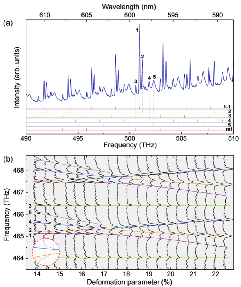
Figure 1: (Color on line) (a) For a COM with $\eta$=18.7%, five uncoupled mode groups are identified. (b) Several ACs are observed as we vary $\eta$ when modes are followed adiabatically. Inset: the spectrum measured with a spectrometer with a higher resolution ($\sim$0.012 THz), resolving AC of two adjacent modes.

Outside the frequency range of Fig. 1(a), however, some of the modes from different mode sequences would get very close because of their different $\Delta\nu$’s and they would interact and repel each other due to the coupling introduced by ray chaos as to be seen later. Even in this case, we can extend our labeling over the entire spectral range of measurement (420 THz - 530 THz) by employing the conventional assumption of adiabatic change in $\Delta\nu$ of a given mode sequence from one FSR to another. In order to distinguish this mode-sequence label from the mode order defined above, we use a different notation $l$, called mode label, such that $l$ coincide with $l_{0}$ only in the above limited region of frequency.

CMF and lasing spectra similar to that in Fig. 1(a) have been measured for various $\eta$ values from 10% to 23% and all of the observed modes are labeled by the convention explained above. A part of the results are shown in Fig. 1(b), where we can see some of encountering modes ($l$=2 mode and $l$=4 mode, $l$=1 mode and $l$=2 mode) undergo ACs as the cavity deformation is varied.

In order to investigate mode dynamical properties at a fixed deformation, we now introduce an internal parameter $n$ indexing the recurring modes in a given mode sequence. The usefulness of $n$ is obvious when we consider the quasi-eigenmodes of a deformed cavity, obtained by diagonalizing a two-state effective Hamiltonian matrix (with $\hbar$=1),

$$H(n,\eta)=\left[\begin{array}[]{cc}\nu_{p}(n,\eta)-i\gamma_{p}(\eta)&C_{pq}(\eta)\\ C_{pq}(\eta)&\nu_{q}(n,\eta)-i\gamma_{q}(\eta)\end{array}\right],$$ (3)

where $\nu_{p(q)}$ and $\gamma_{p(q)}$ are frequencies and decay rates of two uncoupled states with different mode orders, respectively, and $C_{qp}$ is the internal coupling induced by cavity deformation. This coupling is taken to be real because it arises mainly from internal ray dynamics in our experiment as to be shown later. AC along $\eta$ as shown in Fig. 1(b) then takes place at $\eta_{0}$ satisfying $\nu_{p}(n,\eta_{0})=\nu_{q}(n,\eta_{0})$ for a given $n$ if $C_{pq}>|\gamma_{p}-\gamma_{q}|/2$, a criterion for AC. Now we consider the variation of $n$ at a given $\eta^{\prime}(\neq\eta_{0})$ instead. Since states with different mode orders have different $\Delta\nu$’s, there exists some $n_{0}$ satisfying $\nu_{p}(n_{0},\eta^{\prime})\simeq\nu_{q}(n_{0},\eta^{\prime})$, for which an AC can take place. We assume that both decay rate $\gamma_{p(q)}$ and coupling strength $C_{pq}$ are independent of $n$ since their dependence on frequency is not substantial in the frequency range studied.

Mode-dynamics diagrams in Fig. 2 are based on this idea of scanning $n$. We first define reference frequencies as the resonance frequencies of $l_{0}$=3 whispering-gallery modes in a circular cavity whose round trip length is the same as that of the COM under investigation. These reference frequencies are shown as equally-spaced vertical ticks marked as ‘ref’ in Fig. 1(a). We then measure the relative frequencies of the observed quasi-eigenmodes corresponding to $n$ with respect to the reference frequency of the same $n$ for a given $\eta$, and plot these relative frequencies as a function of the reference frequency corresponding to $n$. Mode-dynamics can be analyzed more effectively in a mode-dynamics diagram than in Fig. 1(b) since we can then associate the observed mode dynamics to the relevant phase-space structure for intracavity ray dynamics, the so-called Poincáre surface of section (PSOS), for a given $\eta$.

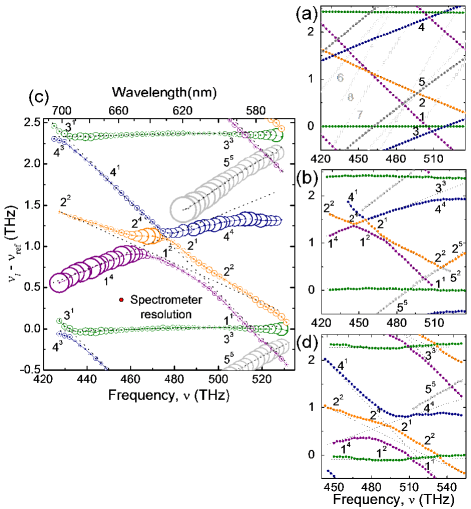
Figure 2: (Color online) (a) Calculated relative frequencies of quasi-eigenmodes with radial mode order $l_{0}$=1, 2, $\cdots$, 8 for a circular cavity ($\eta$=0%) with the mode frequency of $l_{0}$=3 as a reference. (b) Observed relative frequencies of quasi-eigenmodes for $\eta$=14.3%. Mode frequencies more or less follow diabatic lines (dotted straight lines) except for ACs with very small splittings. We employ shorthand notation $l^{l_{0}}$ as explained in the text. (c) The same for $\eta$=18.7%. More pronounced ACs with decay-rate exchange as well as ordinary crossings are observed. The diameter of the circle drawn on each data point represents the half linewidth of the corresponding mode in THz. Red circle indicates spectrometer resolution, $\gamma_{0}\sim$ 0.05 THz. (d) The case of $\eta$=22.3%. The splittings are much more larger than those of (c) and the mode frequencies deviate greatly from the diabatic lines.

Note in Figs. 2(b)-(d) that when these quasi-eigenmodes are far apart they follow straight lines called diabatic transition lines Takami02 even in the presence of the internal coupling $C$ [the case of Fig. 1(a)]. By shifting the internal parameter $n$, we can bring any two quasi-eigenmodes get close and make the internal coupling come into play. In this case, the quasi-eigenvalues deviate from the diabatic lines significantly, exhibiting ACs. Note also that the mode order $l_{0}$ is associated with the uncoupled states located on the diabatic lines (straight lines in Fig. 2), while the mode index $l$ is associated with quasi-eigenmodes on adiabatic lines (exhibiting ACs in Fig. 2). The shorthand notation $l^{l_{0}}$ such as $1^{2}$ in Fig. 2 is based on this idea. Furthermore, by comparing Fig. 2(a) in the case of circle with Figs. 2(b)–2(d) for deformed cavities, we can recognize that the modes on the $l_{0}$th diabatic line must have evolved from the WGM’s of radial quantum number $l_{0}$ of a circular cavity.

The diameter of the circle drawn on each data point in Fig. 2(c) represents the half linewidth in THz, directly observed with a spectrometer. It is reassuring to see that the linewidth well before and well after an avoided crossing is continuous along the diabatic transition line, which is a general property of avoided crossing Takami02 . On the other hand, in the region where avoided crossings occur, the linewidth is an intermediate value of those well before and well after the avoided crossing.

Another important factor to consider in Fig. 2 is the parity of mode. Only modes with the same parity can interact with each other. In the frequency range of $\nu\sim$500 THz and $0<\nu_{l}-\nu_{\rm ref}<$2.25 THz, uncoupled states of $l_{0}$=3 and 5 have a parity different from that of $l_{0}$=1, 2, and 4 states of the same $n$. This feature has been confirmed by mode calculations by boundary element method Wiersig03 ; Shim07 . This is why quasi-eigenmodes originating from $l_{0}$=1, 2 and 4 states avoid each other there and why $l_{0}$=1 and 2 states cross the $l_{0}$=3 state near ($\nu,\nu_{l}-\nu_{\rm ref}$)$\sim$(510, 0)(THz) in Figs. 2(b)–2(d). However, the same $l_{0}$=1 state and another $l_{0}$=3 state displaced by one FSR result in quasi-eigenstates undergoing an AC near (430, 2.3)(THz) since any state with its mode number shifted by one ($n\rightarrow n\pm 1$) would have its parity changed to the other parity tureci02 .

By the same reason one may expect that the same $l_{0}$=1 state and another $l_{0}$=5 state with an one-less mode number would result in an AC near (525, -0.25)(THz) in Figs. 2(c), (500, 0.25)(THz) in Figs. 2(b), and (540, 1.4)(THz) in Figs. 2(d). However, they all exhibit a crossing instead. It is because $C_{15}<|\gamma_{5}-\gamma_{1}|/2$, not satisfying the criterion for AC. This example demonstrates that openness can suppress the AC in the present internal coupling case. From this openness effect, we can expect that the level spacing distribution would show a delayed transition from Poisson to Wigner-like distribution in the chaotic transition.

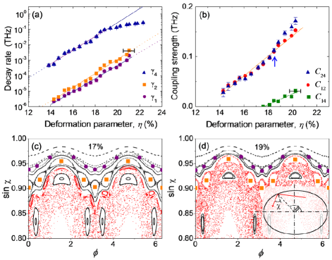
Figure 3: (Color online) (a) Decay rates $\gamma_{p}$ of $p$=1,2,4 uncoupled states. (b) Coupling strength $C_{pq}$ between $p,q$(=1,2,4) uncoupled states, restored from the observed sizes of AC and the decay rates of modes, assuming three-mode coupling. Systematic error in determining exact deformation is indicated with a horizontal error bar in both (a) and (b). (c) PSOS’ for $\eta$=17% and (d) $\eta$=19%. Large (purple) circular and (orange) square dots represent the classical trajectories that $l_{0}$=1 and 2 modes would correspond to, respectively, whereas that of $l_{0}$=4 mode is embed in the chaotic sea below. Inset: Birkhoff coordinates used in PSOS’.

From the observed gaps of AC and the associated decay rates of corresponding uncoupled states [Fig. 3(a)], we can finally reconstruct the internal coupling strength $C(\eta)$ between encountering modes as shown in Fig. 3(b). In the present case, all three $l_{0}$=1,2,4 modes of the same parity are coupled to each other since their mode frequencies are not much separated in the region of interaction. The reconstructed coupling strengths, $C_{12},C_{24},C_{14}$, summarized in Fig. 3(b) are obtained by diagonalizing a three-mode non-Hermitian symmetric Hamiltonian, a straightforward extension of Eq. (1). It is the first time to directly measure mode-mode coupling constants in an open chaotic billiard of generic nonintegrable shape. In Fig. 3(b) these couplings are shown to increase as the degree of deformation increases.

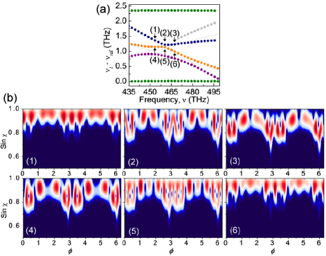
Figure 4: (Color online) (a) Calculated relative frequencies of $l$=1, 2, 3, 4, 5 modes with respect to the reference frequency. (b) Hisimi plots of the modes marked by arrows near 460 THz where $l$=2, 4 modes undergo an AC.

Unfortunately, there is no known semiclassical theory for enabling us to calculate the observed coupling constants. At best, they can be understood qualitatively in terms of classical ray dynamics in phase space. Following this standard practice we plot PSOS in Figs. 3(c) and 3(d), for $\eta$=17% and 19%, respectively, by using the Birkhoff coordinates with $\phi$ the polar angle and $\chi$ the incident angle in ray tracing analysis Lee02 . Large (purple) circular and (orange) square dots represent the classical trajectories that $l_{0}$=1 and 2 modes would correspond to, respectively, whereas that of $l_{0}$=4 mode is embedded in the chaotic sea for the shown degrees of deformation. These trajectories are inferred from phase-space distributions or Husimi plots of the these modes Lee07PRA . When $\eta>18\%$, as shown in Fig. 3(d), the classical trajectory associated with $l_{0}$=2 mode no longer lie on the main integrable region, separated from the chaotic sea by unbroken Kolmogorov-Arnold-Moser (KAM) curve, as it did in Fig. 3(c) for $\eta$=17%, but lie on islands surrounded by chaotic sea, and thus chaotic diffusion starts to play an important role for the increased coupling $C_{24}$ between $l_{0}$=2 and 4 modes as shown in Fig. 3(a). The broken KAM curve is also responsible for the increased coupling $C_{14}$ between $l_{0}$=1 and 4 modes.

The observed mode-dynamics diagrams have also been reproduced by numerical calculations based on the boundary element method Wiersig03 ; Shim07 applied for the same shape and size of the cavity as in the experiment. The eigenvalues and associated Husimi distributions calculated for $\eta$=0.19 are shown in Fig. 4, where we confirm that the encountering quasi-eigenmodes exchange their mode distributions upon avoided crossing [(1)$\leftrightarrow$(6) and (4)$\leftrightarrow$(3)] and at the closest encounter the resulting modes [(2) and (5)] are linear superpositions of the modes well before and well after the avoided crossing, thus leading to delocalized eigenfunctions Takami02 ; Noid83 .

In conclusion, we have developed an spectroscopic technique to enable experimental investigation of mode-dynamics evolution along the chaotic transition in open chaotic billiards. The observed mode-dynamics evolution shows that openness tends to suppress avoided crossings compared to the closed billiard cases. We could directly measure the coupling strengths induced by ray chaos among encountering modes. Our measurements would serve as a valuable asset for anticipated but currently-nonexisting semiclassical theory for coupling strengths between modes in a mixed phase space.

This work was supported by National Research Laboratory Grant and by WCU Grant. S.W.K. was supported by KRF Grant (2006-005-J02804) and by KOSEF Grant (R01-2005-000-10678-0). S.Y.L. was supported by BK21 program.

References

- (1) H.-J. Stöckmann, Quantum Chaos: an Introduction (Cambridge Univ. Press, Cambridge, 1999).
- (2) H.-J. Stöckmann and J. Stein, Phys. Rev. Lett. 64, 2215 (1990); H.-D. Gräf et al., Phys. Rev. Lett. 69, 1296 (1992).
- (3) A. Bäcker et al., Phys. Rev. Lett. 100, 174103 (2008).
- (4) E. Persson, I. Rotter, H. -J. Stöckmann, and M. Barth, Phys. Rev. Lett. 85, 2478 (2000).
- (5) C. Dembowski et al., Phys. Rev. Lett. 86, 787 (2001).
- (6) J. U. Nöckel, A. D. Stone, G. Chen, H. L. Grossman, and R. K. Chang, Opt. Lett. 21, 1609 (1996).
- (7) J. Yang et al., Rev. Sci. Instrum. 77, 083103 (2006).
- (8) S. Moon et al., Optics Express 16, 11007 (2008).
- (9) S.-B. Lee, J.-H. Lee, J.-S. Chang, H.-J. Moon, S. W. Kim, K. An, Phys. Rev. Lett. 88, 033903 (2002).
- (10) S.-B. Lee et al., Phys. Rev. A 75, 011802(R) (2007).
- (11) T. Takami, Phys. Rev. Lett. 68, 3371 (1992).
- (12) J. Wiersig, J. Opt. A 5, 53 (2003).
- (13) J.-B. Shim et al., J. Phys. Soc. Jpn. 76, 114005 (2007).
- (14) H. E. Tureci, H. G. L. Schwefel, A. D. Stone, and E. E. Narimanov, Opt. Exp. 10, 752 (2002).
- (15) D. W. Noid, M. L. Koszykowski, and R. A. Marcus, J. Chem. Phys. 78, 4018 (1983).