Evolution of the u-band luminosity function from redshift 1.2 to 0

Abstract

We produce and analyse u-band ($\lambda\approx 355$ nm) luminosity functions for the red and blue populations of galaxies using data from the Sloan Digital Sky Survey (SDSS) u-band Galaxy Survey (uGS) and Deep Evolutionary Exploratory Probe 2 (DEEP2) survey. From a spectroscopic sample of 41 575 SDSS uGS galaxies and 24 561 DEEP2 galaxies, we produce colour magnitude diagrams and make use of the colour bimodality of galaxies to separate red and blue populations. Luminosity functions for eight redshift slices in the range $0.01<z<1.2$ are determined using the $1/V_{max}$ method and fitted with Schechter functions showing that there is significant evolution in $M^{*}$, with a brightening of 1.4 mags for the combined population. The integration of the Schechter functions yields the evolution in the u-band luminosity density out to $z\sim 1$. By parametrizing the evolution as $\rho\propto(1+z)^{\beta}$, we find that $\beta=1.36\pm 0.2$ for the combined populations and $\beta=2.09\pm 0.2$ for the blue population. By removing the contribution of the old stellar population to the u-band luminosity density and correcting for dust attenuation, we estimate the evolution in the star formation rate of the Universe to be $\beta_{SFR}=2.5\pm 0.3$. Discrepancies between our result and higher evolution rates measured using the infrared and far-UV can be reconciled by considering possibilities such as an underestimated dust correction at high redshifts or evolution in the stellar initial mass function.

1 Introduction

The evolution in the star formation rate (SFR) of the Universe over the course of cosmic history is a measure of great importance that has many applications in various fields of astrophysics. In addition to the obvious applications to the build-up of stellar mass in galaxies, other examples include constraining the stellar initial mass function (IMF) (Baldry & Glazebrook, 2003; Wilkins et al., 2008), testing models of chemical evolution in the Universe (Calura & Matteucci, 2004), constraints on the nature of both type Ia supernovae (Strolger et al., 2004) and gamma-ray bursts (Daigne et al., 2006; Li, 2008) and comparisons with global AGN activity and the growth of black holes (Franceschini et al., 1999; Somerville et al., 2008).

SFRs of galaxies have been measured by a variety of methods, at different wavelengths. These include: SFRs determined from the far- and mid-infrared produced by the re-emission of ultraviolet (UV) photons by dust grains, revealing hidden star formation (Le Floc’h et al., 2005; Pérez-González et al., 2005); SFRs measured from radio emission produced by relativistic electrons in supernova remnants (Condon, 1992; Seymour et al., 2008); Nebular emission lines such as ${\rm H_{\alpha}}$, ${\rm H_{\beta}}$ and ${\rm[OII]}$, produced by the recombination of ionized gas surrounding hot young OB stars (Kennicutt & Kent, 1983; Moustakas et al., 2006; Cooper et al., 2008; James et al., 2008a); and X-ray emission produced by X-ray binary systems in late-type galaxies (Norman et al., 2004; Lehmer et al., 2008).

More directly, SFRs have been measured from the UV luminosities of galaxies produced from short lived OB stars (lifetimes $\sim 10^{7}$ yr). Early studies such as Lilly et al. (1996) and Madau et al. (1996) used this to establish that the volume-averaged SFR of the Universe has been in decline since $z\sim 1$ to the present day. Although later studies (Madau et al., 1998; Steidel et al., 1999; Wilson et al., 2002) measured the decline with improved precision, it is still poorly constrained and its cause is still a major problem in the field of observational cosmology.

As an alternative to the far UV luminosity, the u-band ($\lambda\approx 355$ nm) luminosity of a galaxy, predominantly emitted by young stars of ages $<1$ Gyr, has been shown to be a reasonable tracer of star formation (Hopkins et al., 2003). Using u-band has two main advantages over the far UV, because i) more data are available to improve the statistics and ii) it is less affected by extinction. Driver et al. (2008) find that at $z=0$, the fraction of photons to escape through the dust from the local galaxy population is $\sim 45$ per cent in the u-band as opposed to $\sim 25$ per cent at 200-nm. One disadvantage of the u-band as a tracer of star formation is the contribution from old stellar populations, which is dominant in early-type galaxies and small in star forming galaxies. This has to be accounted for.

So far u-band field luminosity functions (LFs) have been produced by Blanton et al. (2003b) for Data Release 2 (DR2) of the Sloan Digital Sky Survey (SDSS) main sample, by Baldry et al. (2005) for the SDSS u-band Galaxy Survey (uGS) and more recently by Montero-Dorta & Prada (2008) using DR6, probing volumes out to $z\sim 0.2$. In this paper we extend the analysis to higher redshift, by combining samples of galaxies taken from the SDSS uGS and the Deep Evolutionary Exploratory Probe 2 (DEEP2) survey, to produce LFs in the range $0.01<z<1.2$, which represents $\sim 8$ Gyr of cosmic history from when the Universe was $\sim 5$ Gyr old. Selected by R-band, the DEEP2 survey is ideally suited for comparison to the SDSS uGS as R-band magnitudes at $z\sim 1$ correspond to rest u-band magnitudes. We go on to produce colour magnitude diagrams (CMDs) from the data and make use of the observed colour bimodality (Strateva et al., 2001; Baldry et al., 2004) to separate the narrow band of red, passive galaxies and blue star forming populations of galaxies. Integration of the LFs produced from these separate populations allows the luminosity density, or total output of u-band light in a given volume to be determined.

The structure of this paper is as follows: Section 2 describes the DEEP2 Survey and SDSS uGS, and the data reduction employed to obtain our final galaxy samples. In section 3 the methods required to calculate the luminosity functions including completeness corrections and K corrections are described, and we present rest-frame CMDs displaying how the red and blue populations are separated. In section 4 we present the luminosity functions, fitted Schechter parameters and luminosity densities. Our results are then compared with the observations at different wavelengths and we discuss our estimate of the evolution of SFR of the Universe in section 5. Section 6 contains a summary of our conclusions. Throughout this paper we adopt a cosmology with parameters $(\Omega_{m},\Omega_{\Lambda})_{0}=(0.3,0.7)$ and $H_{0}=70$ km s^-1 Mpc^-1. Magnitudes are corrected for Galactic extinction using dust maps of Schlegel et al. (1998).

2 Data

2.1 DEEP2

The Deep Evolutionary Exploratory Probe 2 (DEEP2) survey (Davis et al., 2003) is a redshift survey primarily designed to probe the properties of galaxies at redshift z $\sim$ 1. When fully complete the spectra of around 50 000 galaxies with redshifts $z<1.4$ will have been measured over an area of sky totalling 3.5 deg².

In this paper we use data from the third data release, DR3, which comprises two catalogues: photometric and spectroscopic. The photometric catalogue contains the $B,R$ and $I$ magnitudes of 716 465 objects (including stars and duplicate objects) obtained with the $12k\times 8k$ mosaic camera (Cuillandre et al., 2001) on the 3.6 m Canada-France-Hawaii-Telescope. The spectroscopic catalogue contains redshifts and spectra of 46 337 objects measured by the DEIMOS spectrograph (Faber et al., 2003) with wavelength range $600-920$ nm and resolution $\lambda/\Delta\lambda\sim 5000$ on the 10m Keck 2 telescope. Galaxies selected for redshift measurements are limited to apparent AB magnitudes in the range $18.5<R<24.1$.

The survey area is separated into 4 regions of the sky and is made up of a 0.5 sq. deg. field known as the Extended Groth Strip (EGS) and three 1.0 sq. deg. fields designated fields 2, 3 and 4. Galaxies in fields 2, 3 and 4 are preselected by their $B$, $R$ and $I$ magnitudes using colour cuts, to have estimated redshifts $z>0.7$. No such preselection was carried out for the EGS which means that there is an approximately equal number of galaxies below and above $z=0.7$ in this region.

2.2 DEEP2 sample reduction

Before determining the luminosity functions, stars and duplicate objects had to be removed from the DEEP2 catalogues and it was also useful to cut the area of the photometric catalogue, due to the spectroscopic catalogue not yet covering the same area as the photometric catalogue. The methods used to reduce the catalogues to obtain a final sample of galaxies used in this paper are described in this section.

The first reduction of the photometric catalogue was to cut down the areas of the photometric survey in each field, so that the areas of the photometric and incomplete spectroscopic catalogues are the same. 177 680 objects in the photometric catalogue were cut, reducing it to 538 785.

The second procedure was to discard galaxies with magnitudes outside the range $18.5<R<24.1$, to give the spectroscopic and photometric catalogues equal magnitude limits. This removed 313 362 objects from the photometric catalogue and 58 objects from the spectroscopic catalogue. After matching up the spectroscopic object numbers with those in the photometric catalogue, 6 objects were found to have no corresponding object number in the photometric catalogue. These 6 objects were removed from the spectroscopic catalogue. After this reduction the photometric and spectroscopic catalogues contained 225 423 and 46 279 objects respectively.

The third reduction was to remove stars from the catalogue. Objects in the photometric catalogue are designated a quantity, PGAL (Coil et al., 2004), that gives the probability of an observed object being a galaxy or not. This probability is determined from star-galaxy separations calculated from the magnitudes, sizes and colours of the objects. Resolved sources i.e. those which are definitely galaxies are given a PGAL value of 3 whereas unresolved sources are given a probability of being a galaxy between 0 and 1. In this investigation it was decided to use objects with PGAL $>0.2$ as in Willmer et al. (2006).

The final reduction was to remove galaxies in the catalogues that had been observed multiple times and designated different object numbers. These duplicated observations for objects were identified by running a procedure to find and match objects within 0.5 arc-seconds of each other. The matched objects with the best redshift quality and smallest error in $R$ mag, were used to produce the luminosity functions. The duplicate objects with poorer data were then removed from the photometric and spectroscopic catalogues. These two further processes reduced the photometric catalogue by 58 824 to 166 599 galaxies. 629 objects in the spectroscopic catalogue which had object numbers corresponding to galaxies removed from the photometric catalogue, were also removed, leaving 45 650 objects in the spectroscopic catalogue.

The properties of the reduced fields can be seen in Table 1. $N{{}_{P}}$ and $N{{}_{z}}$ are the numbers of galaxies with photometry and spectroscopy. Our primary sample consists of 24 561 galaxies with redshifts in the range $0.4<z<1.2$.

Table 1: Properties of the DEEP2 reduced survey sample

Field	Reduced Area (sq. deg.)	$N{{}_{P}}$	$N{{}_{z}}$
EGS	0.45	36319	13440
Field 2	0.68	34976	9559
Field 3	1.00	52390	11904
Field 4	0.94	42914	10747
Total	3.07	166559	45650

2.3 The SDSS u-band Galaxy Survey

The Sloan Digital Sky Survey is only briefly described here, for greater detail the reader is referred to York et al. (2000) and subsequent data release papers such as the EDR paper (Stoughton et al., 2002). The SDSS is both a photometric and spectroscopic survey which makes use of a dedicated 2.5-m telescope situated on Apache Point, New Mexico. Photometry in 5 broadband filters, ugriz, is conducted using a mosaic CCD camera (Gunn et al., 1998) and calibrated with a 0.5-m telescope (Hogg et al., 2001). Spectra of selected objects are measured using a 640-fibre fed spectrograph with wavelength range 380-920 nm and resolution $\lambda/\Delta\lambda\sim 1800$.

The sample of galaxies used in this paper is taken from ‘Stripe 82’ of the SDSS ‘Southern Survey’ (Adelman-McCarthy et al., 2006). This consists of a $2.52^{\circ}$ wide strip across the Southern Galactic Pole (SGP) centred along the celestial equator from RA $-50.8^{\circ}$ to $58.6^{\circ}$. Multiple imaging passes of the stripe allow co-added $u$-band Petrosian fluxes to be determined. This gives an increase in the S/N ratio by a factor of about 3 over single epoch observations. Extra spectroscopic observations of galaxies (fully described in Baldry et al. 2005) include a low-$z$ $r_{petro}<19.5$ sample and a $u_{select}<20$ sample. The multiple scans, and extra spectra, allow a catalogue of objects to be produced with $u_{petro}<20.5$ based on the co-added data. The result is a photometric catalogue of 75 087 objects, with magnitudes in the range $14.5<u<20.5$ and spectroscopy for 48 640 objects in an area of 275 deg². Our primary sample consists of 41 615 galaxies with redshifts in the range $0.01<z<0.2$.

3 Methods

3.1 Completeness corrections

Completeness corrections are required to correct the luminosity functions for the number of galaxies that are not targeted for spectroscopic observations. For both surveys, empirical completeness values were determined by binning in observed quantities. For the SDSS uGS sample of galaxies it is assumed that all the redshifts are correct but for the DEEP2 data we additionally take into account the redshift success rate, which is explained below.

3.2 DEEP2 completeness

Redshifts in the DEEP2 survey were first determined by an automated pipeline (Cooper et al. 2009, in preparation) which does all the image reduction and extraction of spectra which are then validated by eye. In this process the redshifts were given a quality assessment value (Q) from 1 to 4. Q=1 indicates the redshift determined to be poor due to a lack of features in the spectra, whereas Q=4 means the redshift has two or more identified features (the ${\rm[OII]}$ $\lambda=372.7$ nm doublet is considered to be two features) and the determined redshift is rock solid.

In this paper we only use galaxies with Q $\geq$ 3. To calculate the redshift success, galaxies are divided into bins of $R$ band apparent magnitude from $18.5<R<24.1$. Brighter galaxies with $18.5<R<20.0$ are divided into 0.5 mag bins whereas galaxies with $20.0<R<24.1$ are divided into 0.2 mag bins. The redshift success is then simply the number of galaxies with Q $\geq$ 3 divided by the total number of galaxies per magnitude bin. The redshift success as a function of $R$ band apparent magnitude is shown in Fig. 1.

On inspection of Fig. 1 it is clear that the redshift success drops unexpectedly for the brightest galaxies. After correspondence with Mike Cooper of the DEEP2 collaboration, we have found this is mainly due to some low redshift galaxies that have been incorrectly designated as having too poor quality spectra (to measure a redshift). The DEEP2 team acknowledge this is something that will be corrected for the next data release (DR4). Our completeness corrections assume that the missed redshifts, both bright and faint, have a similar redshift distribution as the obtained redshifts. The overall conclusions of this paper are unlikely to be significantly affected by the validity of this assumption because the completeness is $>0.7$ up to $R\simeq 23$.

Figure 1: Redshift success fraction as a function of apparent $R$-band magnitude for DEEP2 DR3. The redshift success fraction is simply the number of galaxies with redshift quality Q $\geq$ 3 divided by the total number of galaxies, within an apparent $R$-band magnitude bin. Error bars indicate Poisson errors.

A targeting completeness correction accounts for the galaxies that are not targeted for spectroscopy. This is calculated by dividing galaxies in both photometric and spectroscopic catalogues into colour-colour bins. Firstly the galaxies are divided into 39 $R-I$ colour bins between $-3.0<R-I<4.0$. Galaxies are divided in the following bins $[<-0.03,-0.03\rightarrow 1.01$ (binsize 0.04), $1.01\rightarrow 1.56$ (0.05), $>1.56]$. Then the galaxies are subdivided into 61 $B-R$ colour bins. All galaxies lie within the range $-1.6<B-R<7.0$ and are divided into bins $[<-1.0,-1.0\rightarrow 4.9$ (binsize 0.1), $>4.9]$. This is done with the intention of obtaining a few tens of galaxies in each colour-colour bin.

Targeting completeness is simply the number of galaxies from the spectroscopic catalogue divided by the number of galaxies in the photometric catalogue in each colour-colour bin. Fig. 2 shows the distribution of colours for all 166 599 DEEP2 galaxies in the photometric catalogue represented as contours along with the targeting completeness as a function of $R-I$ and $B-R$. From this plot the colour preselection used to obtain galaxies at $z>0.7$ can be clearly seen as the region of moderate completeness (green). In this paper we choose not to treat galaxies within the Extended Groth Strip (EGS) separately from the other DEEP2 fields and an effect of this is the region of galaxies with low completeness (red) also seen in the figure.

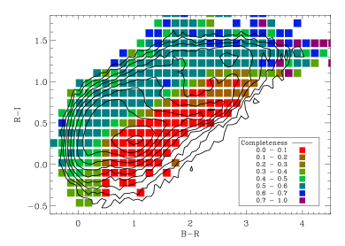
Figure 2: Targeting completeness of DEEP2 galaxies as a function of $R-I$ and $B-R$ colours. The targeting completeness corrects the LFs for galaxies not selected for spectroscopic observations. It is the number of galaxies in the spectroscopic catalogue divided by the number of galaxies in the photometric catalogue, within a colour-colour bin. All four DEEP2 fields are treated the same way regarding targeting completeness. A consequence of this is two distinct regions; a region of moderate completeness consisting of galaxies from fields 2, 3 and 4, having preselected colours to have redshifts greater than 0.7 and a region of low completeness made up of galaxies from the Extended Groth Strip. The distribution of colours for 166 599 DEEP2 galaxies from the photometric catalogue are represented by logarithmically-spaced contours.

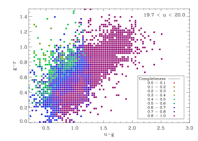
Figure 3: Sample completeness as a function of $g-r$ and $u-g$ colours for the SDSS uGS galaxies with $19.7<u<20.0$. For completeness as a function of $\Delta_{sg}$, u, $u-g$ and $g-r$ see Baldry et al. (2005).

The overall completeness for a single galaxy is simply the product of the redshift success rate and targeting completeness.

3.3 SDSS uGS completeness

Completeness corrections for the SDSS uGS sample are fully described in Baldry et al. (2005). These are determined by dividing the sample into bins using the star-galaxy separation, $\Delta_{sg}$ ($=r_{PSF}-r_{model}$, the difference between r-band point spread function and ‘model’ magnitudes), along with u, $u-g$ and $g-r$ as variables. Firstly the objects are divided into weakly and strongly resolved sources at the dividing line of ${\Delta}_{sg}=0.3$. For $u>19.7$ strongly resolved sources are divided into 0.1 mag bins and weakly resolved sources are divided into 0.2 mag bins. These magnitude bins are then further divided on the basis of $u-g$ and $g-r$ colour bins so that there are around 50 galaxies in each bin. The completeness is simply the fraction of photometric objects that have spectroscopy. The completeness as a function of $g-r$ and $u-g$ colours for galaxies with $19.7<u<20.0$ is presented in Fig. 3. For a more detailed figure showing the completeness as a function of $\Delta_{sg}$, u, $u-g$ and $g-r$ see Fig. 6 of Baldry et al. (2005). Although the completeness can be low ($\sim$ 0.1–0.2) for the faintest blue galaxies with $20.3<u<20.5$, all parts of galaxy colour-colour space over the full magnitude range are sampled.

Figure 4: Colour magnitude diagrams for the four SDSS redshift slices, in the range $0.01<z<0.2$. The number densities are weighted by $1/(V_{max}C_{i})$ and are represented by logarithmic contours. Little evolution is seen in the colour corresponding to the region between red and blue galaxies for all redshift slices. The solid line represents the straight line given by eq.1, that is used to divide the red and blue galaxy populations. The dashed lines represent the magnitude limit of the redshift slice.

Figure 5: CMD contour plots for four DEEP2 redshift slices in the range $0.4<z<1.2$. Number densities are represented as logarithmic contours. The solid line represents the straight line given by eq.1 that is used to divide the red and blue galaxy populations. The dashed lines represent the magnitude limit of the redshift slice.

3.4 K corrections and colour magnitude diagrams

To convert the observed apparent magnitudes of the galaxies to absolute rest-frame magnitudes we make use of the K correction program Kcorrect (version 4.1.4) of Blanton et al. (2003a). For the DEEP2 sample, $B,R$ and $I$ magnitudes (effective wavelengths $\approx$ 439, 660, 813.5 nm) are transformed into rest frame SDSS u and g magnitudes (effective wavelengths 355 and 467 nm).

For the SDSS uGS sample, the observed u and g magnitudes are converted into the rest frame. This process enabled the production of rest frame u-g colour magnitude diagrams (CMDs) for the galaxies in 8 different redshift slices. Fig. 5 shows CMDs produced from SDSS data and Fig. 5 shows CMDs from DEEP2. These are represented as contour plots which are weighted by $1/(V_{max}C_{i})$. Here $V_{max}$ is the maximum comoving volume, within which a galaxy could lie within a redshift slice and within the magnitude limits of the survey (Schmidt, 1968) and $C_{i}$ is the completeness. These plots show the build up in red galaxies over time and that the colour bimodality of galaxies extends out to $z\sim 1$, as found by Bell et al. (2004), Willmer et al. (2006), Cirasuolo et al. (2007), Franzetti et al. (2007) and Cowie & Barger (2008).

On inspection of the DEEP2 and SDSS uGS contour plots, we find although both blue and red populations are brightening in u-band magnitude as redshift increases, there is no obvious evolution in $u-g$ colours for the natural dividing line. This lack of evolution has also been observed by Cowie & Barger (2008) in AB3400-AB4500 colours out to $z=1.5$ and Willmer et al. (2006) in $U-B$ colours. Given this lack of change, red and blue galaxies at all redshifts can be separated by a straight line with the equation:

$$u-g=-0.033M_{u}+0.75$$ (1)

Changing this dividing line will have little effect on the overall results, as long as it remains in the gap between blue and red populations.

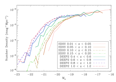
Figure 6: Evolution of the u-band luminosity function for the combined red and blue populations of galaxies. LFs are produced for four redshift slices between $0.01<z<0.2$ for the SDSS uGS data and four redshift slices between $0.4<z<1.2$ for DEEP2, using the non-parametric $1/V_{max}$ method. Galaxies are binned in 0.2 mag bins.

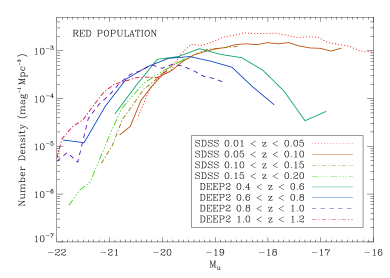
Figure 7: Evolution of the u-band luminosity function for the red population of galaxies. 0.2 mag bins are used to produce all the LFs apart from the $0.4<z<0.6$ and $0.6<z<0.8$ DEEP2 redshift slices where 0.4 mag binning is used.

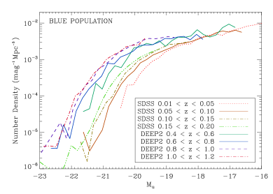
Figure 8: Evolution of the u-band luminosity function for the blue population of galaxies. 0.2 mag binning is used throughout.

4 Results

4.1 Luminosity functions

The luminosity function (LF) is defined as the number of galaxies per unit volume per unit luminosity interval ${\rm d}l$, or alternatively magnitude interval, ${\rm d}M$. In this paper we calculate LFs by the $1/V_{max}$ method, where $V_{max}$ is defined above. This method is non-parametric and does not require any assumptions on the shape of the LF. It can be biased however if there are strong density inhomogeneities in the field. The luminosity function is estimated as follows with the number of galaxies per Mpc³ per absolute magnitude bin given by:

$$\phi(M)=\frac{1}{\Delta M}\sum_{i}^{{N}_{g}}\left(\frac{1}{{C}_{i}\>{V}_{max,i}}\right)$$ (2)

where $C_{i}$ is the completeness for each galaxy described in the previous section.

LFs were produced for the red, blue and combined populations of galaxies, for the same 8 redshift slices as the CMDs above. For the SDSS uGS data we produced LFs for 4 redshift slices over the range $0.01<z<0.2$. For the DEEP2 data we produced LFs for 4 redshift slices between $0.4<z<1.2$. The data were binned in u-band mag bins of width 0.2 mags, apart from the DEEP2 red population, $0.4<z<0.6$ and $0.6<z<0.8$ slices, where 0.4 mag binning was used. The properties of the redshift slices including the numbers of galaxies in the different populations and volumes can be seen in Table 2. Figs. 6, 7 and 8 show the binned LFs for the 8 redshift slices plotted together for the combined, red and blue populations of galaxies. The LFs of all the different populations show a shift to higher luminosities at greater redshift.

By binning the galaxies into 8 redshift slices it ensures that there is reasonable resolution of the evolution ($\sim$ 10 per cent in luminosity per SDSS slice and $\sim 20$ per cent in the DEEP2 slices). It also ensures there are sufficient galaxies to produce LFs with good signal to noise after dividing into the red and blue populations. This is something particularly important for the 0.4–0.6 DEEP2 slice which has fewer galaxies.

Table 2: Spectroscopic sample properties

Redshift Slice	Sample	$N{{}_{ALL}}$	$N{{}_{RED}}$	$N{{}_{BLUE}}$	Volume ($10^{6}$ Mpc3)
0.01-0.05	SDSS	6174	1708	4466	0.263
0.05-0.10	SDSS	14002	4414	9588	1.781
0.10-0.15	SDSS	13559	4302	9297	4.614
0.15-0.20	SDSS	7840	1899	5941	8.552
0.40-0.60	DEEP2	1955	316	1639	2.184a
0.60-0.80	DEEP2	6914	1296	5618	3.404
0.80-1.00	DEEP2	9818	1363	8455	4.488
1.00-1.20	DEEP2	5874	616	5258	5.374

^aThis volume applies to all 4 DEEP2 fields, although most galaxies in this redshift slice are contained within the EGS.

For an analysis of the evolution of the LFs, Schechter functions (Schechter, 1976) were fitted to the binned data. The Schechter function is parametrized as:

$$\phi(L)=\frac{{\phi}^{*}}{{L}^{*}}{e}^{-L/{L}^{*}}\left({\frac{L}{{L}^{*}}}\right)^{\alpha}$$ (3)

where: $L^{*}$ ($M^{*}$) is the characteristic luminosity (magnitude) of a galaxy at the ‘knee’ of the function; $\phi^{*}$ is the number density of galaxies around $L^{*}$ and $\alpha$ is the faint-end slope of the function.

Schechter functions are fitted to the LFs using a least-squares fitting method to find the parameters $\phi$, $M^{*}$ and $\alpha$. In order to quantify the evolution we choose to fix the faint-end slope of the LFs for the different populations on the assumption that it remains constant with redshift. This is due to the faint-end slope being poorly sampled in higher redshift slices. The value we take as the faint-end slope is the one that minimises the total ${\chi}^{2}$ over all redshift slices. After doing this we find best fitting faint-end slopes of $\alpha=-1.3$ for the blue population, $\alpha=-0.35$ for the red population and $\alpha=-1.0$ for the combined LFs.

Using a slope of $\alpha=-1.0$ for the combined population LFs is consistent with the results of Blanton et al. (2003b) who used a sample of 22 020 galaxies with $u<18.4$ and in the redshift range $0.02<z<0.14$ from SDSS DR2, to obtain a slope of $\alpha=-0.92\pm 0.07$. Baldry et al. (2005) determined $\alpha=-1.05\pm 0.08$ for $z<0.06$ and more recently Montero-Dorta & Prada (2008) used a much larger sample of 192 068 galaxies from SDSS DR6, with $16.45<u<19.0$ and a redshift range $0.02<z<0.19$, to obtain a slope of $\alpha=-1.01\pm 0.03$.

Using photometric redshifts from the COMBO-17 Survey Wolf et al. (2003), produce near-UV (280-nm) LFs for 25 000 galaxies in the range $0.2<z<1.2$, as a function of SED type. This study finds no evolution in the faint-end slope for 4 different SED types. For reddest SED type 1 galaxies, the faint-end slope is found to be $\alpha=-0.5\pm 0.2$ and for the the bluest, SED type 4 galaxies a slope of $\alpha=-1.5\pm 0.06$ is found.

Ilbert et al. (2005) using first epoch data from the VIMOS-VLT Deep Survey (VVDS) (Le Fèvre et al., 2004), measure an evolution in the faint end-slope of the U-band LF and find that it steepens from $\alpha=-1.05\pm 0.05$ in the range $0.05<z<0.2$ to $\alpha=-1.44\pm 0.2$ in the range $0.8<z<1.0$. In our study we do not observe this steepening, but in fact the opposite, with $z=0.4$–0.8 DEEP2 redshift slices having shallower slopes than the SDSS slices (if fitted separately).

While allowing $\alpha$ to vary provides a better fit to the data, it should be noted that the galaxies with the faintest magnitudes within each slice have the largest volume and completeness corrections. In particular, the faint DEEP2 data have a low redshift success rate and the assumption that the missed redshifts have the same distribution is a significant source of uncertainty (cf. the ‘average’ model of Faber et al. 2007). The focus of this paper is on extracting reliable luminosity densities, and evolution in $M^{*}$ is more robustly determined using fixed $\alpha$ given the well-known degeneracy in the $M^{*}$-$\alpha$ plane.

The Schechter function fits for the red, blue and combined populations can be seen in Figs. 9 and  10. Errors on the number density used in the fitting process and shown in the figures are Poisson errors added with an error of 5 per cent of the number density, in quadrature, to take into account systematic uncertainties in the binning process. Dotted lines in the figures represent the regions outside the magnitude ranges used to fit the Schechter function. It is notable that while a constant value of $\alpha$ is suitable to describe the evolution of the blue and combined population LFs, there is a deficit of faint red galaxies below the Schechter fit in the higher-redshift DEEP2 data (cf. evolution of the field dwarf-to-giant ratio, Gilbank & Balogh 2008). The main focus of this paper, however, is on the blue sequence and its relationship to cosmic SFR evolution. Tables 3, 4 and 5 display how the fitted Schechter parameters evolve along with the luminosity density (described in the next subsection) from an integration of the LF ($\rho_{FIT}$) and from a summation of the luminosities of all the galaxies ($\rho_{SUM}$).

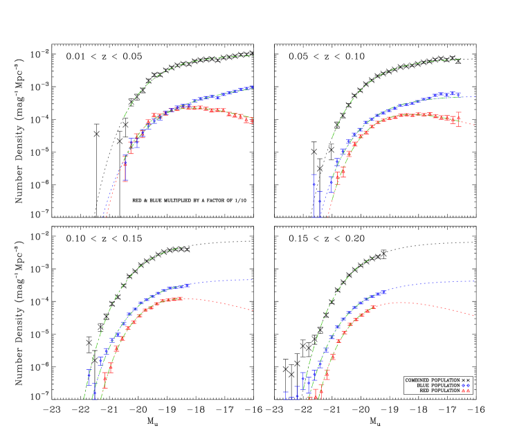
Figure 9: Luminosity functions of the four SDSS uGS redshift slices, for the red, blue and combined populations of galaxies, produced using the $1/V_{max}$ method. The dotted lines show an extrapolation of the Schechter function beyond the fitted magnitude range. The LFs for the red and blue populations are scaled down by a factor of 10. Errors on the data points are Poisson errors added in quadrature to an error of 5 per cent of the number density, to take into account systematic uncertainties in the binning process. $\alpha$ is fixed at $-0.35$, $-1.3$ and $-1.0$ for the red, blue and combined populations respectively.

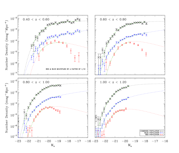
Figure 10: Luminosity functions for the four DEEP2 redshift slices, for the red, blue and combined populations of galaxies. For details see Fig. 9. Note the deficit of faint red galaxies below the fit for three redshift slices because $\alpha$ is constrained by the lowest two SDSS slices.

Table 3: Schechter function parameters for all galaxies with an assumed $\alpha=-1.0$.

$<z>$	$N{{}_{GAL}}$	$M{{}^{*}}$	$\phi{{}^{*}}$ ($10^{-4}$ gal Mpc-3)	$\log\rho_{FIT}$ (W Hz-1 Mpc-3)	$\log\rho_{SUM}$ (W Hz-1 Mpc-3)
0.030	6174	–18.89 $\pm$ 0.03	103.68 $\pm$ 2.55	19.21 $\pm$ 0.01	19.23 $\pm$ 0.01
0.075	14002	–19.12 $\pm$ 0.02	81.60 $\pm$ 1.79	19.19 $\pm$ 0.01	19.17 $\pm$ 0.05
0.125	13599	–19.27 $\pm$ 0.02	80.57 $\pm$ 2.55	19.25 $\pm$ 0.01	19.10 $\pm$ 0.03
0.175	7840	–19.44 $\pm$ 0.02	73.96 $\pm$ 3.78	19.28 $\pm$ 0.02	19.00 $\pm$ 0.05
0.500	1955	–19.80 $\pm$ 0.05	69.71 $\pm$ 2.74	19.41 $\pm$ 0.02	19.42 $\pm$ 0.05
0.700	6914	–20.07 $\pm$ 0.03	63.71 $\pm$ 1.99	19.46 $\pm$ 0.01	19.44 $\pm$ 0.03
0.900	9818	–20.18 $\pm$ 0.02	75.32 $\pm$ 2.27	19.59 $\pm$ 0.01	19.48 $\pm$ 0.13
1.100	5874	–20.28 $\pm$ 0.03	69.17 $\pm$ 2.90	19.59 $\pm$ 0.02	19.39 $\pm$ 0.14

Table 4: Schechter function parameters for red galaxies with an assumed $\alpha=-0.35$.

$<z>$	$N{{}_{GAL}}$	$M{{}^{*}}$	$\phi{{}^{*}}$ ($10^{-4}$ gal Mpc-3)	$\log\rho_{FIT}$ (W Hz-1 Mpc-3)	$\log\rho_{SUM}$ (W Hz-1 Mpc-3)
0.030	1708	–18.60 $\pm$ 0.03	60.91 $\pm$ 1.74	18.82 $\pm$ 0.01	18.82 $\pm$ 0.12
0.075	4414	–18.69 $\pm$ 0.02	38.80 $\pm$ 0.93	18.66 $\pm$ 0.01	18.65 $\pm$ 0.07
0.125	4302	–18.85 $\pm$ 0.02	33.66 $\pm$ 1.21	18.67 $\pm$ 0.02	18.57 $\pm$ 0.03
0.175	1899	–19.07 $\pm$ 0.03	25.56 $\pm$ 1.71	18.62 $\pm$ 0.03	18.42 $\pm$ 0.08
0.500	316	–19.37 $\pm$ 0.08	20.85 $\pm$ 1.62	18.67 $\pm$ 0.03	18.69 $\pm$ 0.08
0.700	1296	–19.44 $\pm$ 0.06	26.06 $\pm$ 3.07	18.78 $\pm$ 0.05	18.71 $\pm$ 0.05
0.900	1363	–19.71 $\pm$ 0.04	16.28 $\pm$ 0.85	18.69 $\pm$ 0.02	18.60 $\pm$ 0.14
1.100	616	–20.07 $\pm$ 0.05	9.52 $\pm$ 0.77	18.60 $\pm$ 0.04	18.48 $\pm$ 0.14

Table 5: Schechter function parameters for blue galaxies with an assumed $\alpha=-1.3$.

$<z>$	$N{{}_{GAL}}$	$M{{}^{*}}$	$\phi{{}^{*}}$ ($10^{-4}$ gal Mpc-3)	$\log\rho_{FIT}$ (W Hz-1 Mpc-3)	$\log\rho_{SUM}$ (W Hz-1 Mpc-3)
0.030	4466	–19.03 $\pm$ 0.05	44.50 $\pm$ 1.73	19.01 $\pm$ 0.02	19.01 $\pm$ 0.09
0.075	9588	–19.09 $\pm$ 0.02	57.60 $\pm$ 1.47	19.03 $\pm$ 0.01	19.01 $\pm$ 0.04
0.125	9297	–19.28 $\pm$ 0.02	53.73 $\pm$ 1.86	19.09 $\pm$ 0.02	18.94 $\pm$ 0.03
0.175	5941	–19.51 $\pm$ 0.02	47.85 $\pm$ 2.60	19.12 $\pm$ 0.02	18.87 $\pm$ 0.05
0.500	1639	–20.17 $\pm$ 0.06	32.64 $\pm$ 1.67	19.34 $\pm$ 0.02	19.33 $\pm$ 0.04
0.700	5618	–20.37 $\pm$ 0.04	33.34 $\pm$ 1.24	19.42 $\pm$ 0.02	19.35 $\pm$ 0.03
0.900	8455	–20.39 $\pm$ 0.03	48.23 $\pm$ 1.72	19.59 $\pm$ 0.02	19.42 $\pm$ 0.13
1.100	5258	–20.46 $\pm$ 0.03	49.13 $\pm$ 2.43	19.62 $\pm$ 0.02	19.34 $\pm$ 0.14

4.2 Luminosity density

After fitting Schechter functions to the binned LFs, these can be used to estimate the total comoving luminosity density (LD), with no extinction correction, in each of the redshift slices for the red and blue populations. We assume that the fitted Schechter function is valid outside the fitted magnitude range. The LD is then given in magnitudes per Mpc³ by

$$j=M^{*}-2.5\log[(\phi^{*}/$Mpc$^{-3})\Gamma_{f}(\alpha+2)]$$ (4)

where $\Gamma_{f}$ is the gamma function, and in linear units by

$${\rho}_{L}={10}^{(34.1-j)/2.5}\;$W H{z}$^{-1}$Mpc$^{-3}$$ (5)

Here $j$ is in AB mag Mpc^-3.

Fig. 11 shows the evolution in the integrated Schechter fit LD for the different populations. For the the blue and combined populations, the luminosity density has decreased steadily from redshift 1.2 to the present day. The red population luminosity density appears to be almost constant, a result also found by Bell et al. (2004) and Faber et al. (2007) who conclude this can be explained by passive fading being compensated by a build up in the stellar mass density. Note also that the fit to the evolution for the blue population LD has a lower $\chi^{2}$ than the fit for the red population. This is not surprising because the cosmic variance is larger for the more clustered red population (Somerville et al., 2004). In fact if the larger error bars from $\rho_{SUM}$ (Table 4) are used when fitting, the best fit shows a marginally rising LD with $z$ rather than declining as in the figure.

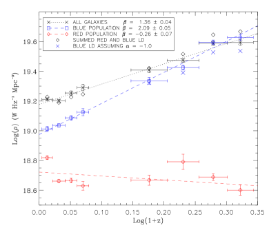
Figure 11: Evolution of the u-band luminosity density for the different galaxy populations. The LD for the combined population is less than the LD for the blue population in the two highest redshift slices. This is due to our fixing the slope of the LF for the different populations. Black diamonds represent the LD obtained from the addition of red and blue LD. Vertical bars indicate $1\sigma$ Poisson errors on the LD. Horizontal bars represent the redshift range. The dashed lines represent fits (eq. 7) to the data. Blue crosses indicate the effects of assuming $\alpha=-1.0$ for the blue DEEP2 population.

As well as calculating the LD from integration of the Schechter fit we also estimate the LD from the summation of the galaxies’ u-band luminosity divided by $1/(V_{max}C_{i})$, in the different redshift slices.

$$\rho_{SUM}=\sum_{i}^{N_{g}}\left(\frac{L_{i}}{C_{i}V_{max,i}}\right)$$ (6)

The values of this summation for the combined, blue and red populations can be found in Tables 3, 4 and 5.

Errors on $\rho_{FIT}$ given in the tables are standard errors from the fitting procedure, while errors on $\rho_{SUM}$ were calculated by dividing the survey areas into sections and finding the standard deviation of $\rho_{SUM}$ between the sections. For the DEEP2 galaxies, we calculated $\rho_{SUM}$ in each of the 4 fields, whereas for the SDSS uGS galaxies we divided the area of the survey into 6 equal areas. The range in magnitudes $\rho_{SUM}$ applies to depends on the magnitude limits of the survey and is always less than the fitted magnitude range of $\rho_{FIT}$. As a consequence the fraction $\rho_{SUM}/\rho_{FIT}$ ranges from 1.05 to 0.53 for the combined sample of galaxies, 1.05 to 0.63 for the red population, and 1.0 to 0.52 for the blue population. This indicates that $\rho_{FIT}$ is never more than a factor of 2 extrapolation from $\rho_{SUM}$. By binning the summed LD in 0.2 mag bins and redshift slices, the contribution of galaxies to the LD, and its evolution as a function of absolute magnitude can be evaluated. Figs. 12, 13 and 14 show this evolution for all, blue and red populations. These plots show peaks that indicate we are sampling galaxies that contribute the most to the luminosity density.

The plots for the combined and blue populations clearly show that as well as the total LD increasing with redshift, the galaxies that contribute most to the LD increase in brightness with redshift. This illustrates ‘downsizing’, first observed by Cowie et al. (1996) and also found in more recent studies (Treu et al., 2005; Bundy et al., 2006), where the brighter, more massive galaxies form their stars at higher redshift than the lower luminosity galaxies. The LD for the red population remains more or less constant over all redshift slices and again the galaxies that contribute most to the LD get brighter with increasing redshift.

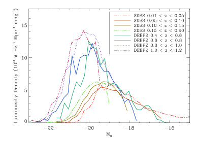
Figure 12: The contribution to the luminosity density for the combined population of galaxies for the 8 redshift slices. The LD is given in units of $10^{18}$ W Hz^-1 Mpc^-3 mag^-1. 0.2 mag binning is used.

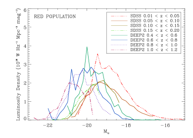
Figure 13: The contribution to the luminosity density for the red population.

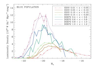
Figure 14: The contribution to the luminosity density for the blue population.

For the combined and blue populations we parametrize the evolution in the integrated LD as in Lilly et al. (1996) by

$${\rho}_{L}\propto(1+z)^{\beta}$$ (7)

For the combined population we obtain $\beta=1.36\pm 0.04$ and for the blue population we obtain $\beta=2.09\pm 0.05$ (assuming a constant faint-end slope $\alpha$). Note if we apply the $\rho_{SUM}$ errors before fitting, we obtain shallower slopes $\beta=1.18$ and 1.95, respectively, and if we apply $\alpha=-1.0$ to the DEEP2 blue population (Fig. 11), the evolution is apparently lower still. Thus, we estimate there is a 0.2 systematic uncertainty in the values of $\beta$ for the combined and blue populations (larger for the red population). In the next section we compare these values of $\beta$ with the results from other surveys at different wavelengths.

5 Discussion

5.1 Comparison between wavelengths

First we compare our results with those from the I-band selected VIMOS-VLT Deep Survey (VVDS) (Le Fèvre et al., 2004). Using a sample of 11 034 galaxies from the first data release of the VVDS, Ilbert et al. (2005) find that $M^{*}$ for rest-frame U-band (360-nm) luminosity function brightens by $\sim 1.8$ mag in the redshift range $0.05<z<1$. This brightening is greater than found in our analysis, which shows that $M^{*}$ for the combined red and blue populations brightens by $\sim 1.4$ mag. Tresse et al. (2007), again using VVDS data, find that the evolution in the U-band luminosity density is fitted by $\beta\approx 1.9$. By combining the LD measurements of Ilbert et al. (2005) with u-band SDSS main sample data from Blanton et al. (2003b), we find that $\beta=1.6\pm 0.4$, which is greater than but consistent with our value of $\beta=1.36\pm 0.2$ for the combined galaxy sample.

In the 150-nm far-ultraviolet (FUV) luminosity functions produced by Arnouts et al. (2005) using Galaxy Evolution Explorer (GALEX) satellite data combined with VVDS, $M^{*}$ was determined to brighten by 2 mag, using a sample of 1 039 galaxies. Schiminovich et al. (2005), using the same data set, find the non-dust corrected luminosity density to evolve with $\beta=2.5\pm 0.7$ out to $z\sim 1$. Wilson et al. (2002) found that the 250-nm, UV LD evolves as $\beta=1.7\pm 1.0$ out to $z\sim 1.5$, using U^′,B,V observations taken as part of a multi-passband survey of the Hubble Deep Field and 4 other fields. Our result along with the other more recent UV measurements rule out the early estimation of the NUV LD evolution by Lilly et al. (1996), who found a steep evolution of $\beta\sim 4$ using the Canada-France-Redshift-Survey (CFRS).

By going to longer wavelengths through optical to the NIR, the light sampled in galaxies is emitted by stars of increasing lifetimes. For the B-band (440-nm), we determined $\beta$ using LD data published in Willmer et al. (2006). This paper made use of an earlier DEEP2 sample of $\sim$ 11,000 galaxies. By fitting to the data we find the LD evolves as $\beta=0.83\pm 0.46$. This is consistent with the combined Blanton et al. (2003b) and Ilbert et al. (2005) measurements, which we find gives an evolution in the B-band of $\beta=1.22\pm 0.28$. These combined results also allow $\beta$ to be estimated for the V, R and I-bands, obtaining $\beta$ values of $1.00\pm 0.32$, $0.82\pm 0.34$ and $0.59\pm 0.34$ respectively.

At near-infrared (NIR) wavelengths, Pozzetti et al. (2003) found from a sample of 489 galaxies in the range $0.2<z<1.3$, that $\beta\approx 0.7$ in the J-band ($1.25\mu$m) and $\beta\approx 0.37$ in the $K_{s}$-band ($2.17\mu$m). This $K_{s}$-band measurement is also consistent with more recent data from the UKIDSS Ultra Deep Survey Early Data Release (Cirasuolo et al., 2007). In this paper LFs are produced for 6 redshift slices in the range $0.25<z<2.25$ using a sample of $\sim$22 000 galaxies. From the LD measured from the first 3 redshift slices, we find that $\beta=0.33\pm 0.38$ in the range $0.25<z<1.25$.

By going to still longer wavelengths in the mid-infrared, obscured star formation can be traced from light re-emitted by dust grains. From mid-infrared 12 $\mu$m data, LFs out to $z\sim 3$ have been produced from observations using Spitzer by Pérez-González et al. (2005) for a sample of $\sim$ 8000 galaxies. From these measurements the evolution in LD obtained from their own form of the luminosity function out to $z\sim 1$ is best fitted by $\beta=3.83\pm 0.26$. Le Floc’h et al. (2005) using Spitzer MIPS 24 $\mu$m data for 2600 sources, converted into total IR luminosities find that the total IR luminosity density evolves as $\beta=3.9\pm 0.4$.

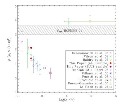
Figure 15: Comparison of non dust corrected LD evolution measured at different wavelengths. Values from Schiminovich et al. (2005), Wilson et al. (2002), Baldry et al. (2005) and Le Floc’h et al. (2005) were plotted directly from the literature. Blanton et al. (2003b) and Ilbert et al. (2005) LD results were combined and $\beta$ calculated from a fit. Pozzetti et al. (2003) is an estimate quoted in their paper and has no errors. $\beta$ was calculated for Willmer et al. (2006), Pérez-González et al. (2005) and Cirasuolo et al. (2007) using LD values at different redshifts and fitting. The error bars for these points are $1\sigma$ errors from the fit. The shaded region indicates the evolution of the star formation rate estimated from multiwavelength data (Hopkins, 2004). For Le Floc’h et al. (2005) we indicate the range of wavelengths that make up the total IR.

Fig. 15 summarises the above results of how the luminosity density evolution ($\beta$) varies as a function of wavelength. As wavelength increases from the far UV to the near infrared, $\beta$ decreases, which is because of the increasing contribution from older stellar populations to the luminosity of the galaxies. This plot clearly shows the difference between our results for the evolution of the u-band LD for the blue and combined populations and the evolution of the infrared LD (Pérez-González et al., 2005; Le Floc’h et al., 2005). Also shown is the SFR density evolution calculated by Hopkins (2004) using a compilation of X-ray, UV, $[{\rm O}_{II}]$, H_α, H_β, mid-IR, sub-millimetre and radio measurements corrected for dust attenuation where necessary.

5.2 Estimating the cosmic SFH from the u-band LD

Given the colour bimodality of galaxies, there is a natural separation between blue and red populations. We can estimate the evolution in the SFR density of the universe from the u-band LD evolution by considering just the blue population. By doing this we effectively remove most of the contribution of u-band luminosity produced by old stellar populations (passive red galaxies).

In order to obtain an estimate of the evolution in the SFR density, we first have to consider the residual u-band luminosity produced by the old population of stars ($\tau>1$ Gyr) in blue galaxies. To do this we perform an analysis using PEGASE (Fioc & Rocca-Volmerange, 1997) models to determine the contribution of u-band luminosity from young stars with ages $\tau<1$ Gyr old. In these models we assume an IMF of Kroupa (2001), with solar metallicity and constant star formation rate between a formation redshift ($z_{form}$) and an observed redshift ($z_{obs}$). For a model with $z_{form}=6$, the fraction of the u-band luminosity from young stars changes from 0.88 at $z_{obs}=1$ to 0.83 at $z_{obs}=0$. For $z_{form}=3$, the fraction changes from 0.9 at $z_{obs}=1$ to 0.84 at $z_{obs}=0$. The assumption that blue galaxies in general form their stars at a quasi-constant rate can be justified considering that studies, such as Brinchmann et al. (2004), have shown low mass galaxies to have had a roughly constant star formation rate and James et al. (2008b) find the same result for local late-type galaxies. If the fraction of u-band luminosity produced by young stars changes by these amounts from $z=1$ to $z=0$ the evolution in the LD evolution with the contribution from old stellar populations removed is $\beta=2.2\pm 0.2$.

The second correction to estimate the evolution in SFR density is to consider an increase in dust attenuation from $z=0$ to $z=1$, as luminosities of characteristic galaxies at higher redshifts are brighter as found by Cowie et al. (1996) and more luminous/higher SFR galaxies have higher dust attenuation than faint systems (Hopkins et al., 2001). For a simple analysis of how much the dust attenuation increases from $z=0$ to $z=1$, we use the magnitudes of the galaxies contributing the most to the LD at $z=0$ and $z=1$. Using Fig. 14, it can be seen that the main contribution to the luminosity density at $z=1$ peaks at $M_{u}\sim-20.5$ and at $z=0$ it peaks at $M_{u}\sim-19$. Converting these typical galaxy magnitudes into flux, we determine the star formation rate (in ${\rm\ M}_{\odot}$ yr^-1) of the galaxies, uncorrected for dust, using the equation of Hopkins et al. (2001), which is a conversion taken from Cram et al. (1998) multiplied by a factor of 5.5 to account for stars with masses $\leq 5{\rm\ M}_{\odot}$.

$$SFR_{UV}=L_{UV}\,/\,7.14\times 10^{20}\,{\rm WHz^{-1}}$$ (8)

Dust corrected star formation rates are obtained from eq. 7 in Hopkins et al. (2001) using the SFRs of the typical galaxies. The difference between the corrected and uncorrected SFRs gives an effective dust attenuation of $A_{u}\sim 1.0$ mag at $z=0$ and $A_{u}\sim 1.25$ at $z=1$ which equates to photon escape fraction of $\sim 0.40$ at $z=0$ and $\sim 0.32$ at $z=1$. This is comparable to the results of Driver et al. (2008) who find the photon escape fraction to be $\sim 0.45$ using the local galaxies.

This is reasonable as other UV studies such as Buat et al. (2005) find the mean extinction of a GALEX sample of galaxies in the local universe to be $A=1.1$ in the NUV (230-nm) and $A=1.6$ for the 150-nm FUV. The dust corrected evolution in the LD for the blue galaxies is essentially the evolution in the SFR density of the universe excluding dusty star forming red galaxies and possibly the most extreme objects with hidden star formation such as luminous infrared galaxies (LIRGS). Assuming there is an increase in the photon escape fraction of $0.32\pm 0.02$ to $0.40\pm 0.02$ from $z=1$ to $z=0$, this implies that $\beta_{SFR}=2.5\pm 0.3$.

5.3 Further correction for dusty star forming galaxies

After correcting for u-band LD evolution for dust and the residual u-band luminosity from the old stellar populations, the discrepancy still remains between our estimate in the SFR evolution ($\beta_{SFR}=2.5\pm 0.3$) and the results of Hopkins (2004) ($\beta_{SFR}=3.3\pm 0.3$), Le Floc’h et al. (2005) ($\beta_{SFR}=3.9\pm 0.4$) and the evolution in SFR densities we determined using the combination of UV and far IR from Takeuchi et al. (2005) to give $\beta_{SFR}=3.4\pm 0.6$. Possible reasons for the discrepancy include: (i) star formation on the red sequence; (ii) a higher dust attenuation correction for dusty star forming galaxies; (iii) evolution of the IMF.

The first way to resolve the discrepancy would be to take into account the star formation occurring in dusty galaxies on the red sequence. Studies such as Franzetti et al. (2007) find, using first epoch VVDS data, that the fraction of red galaxies ($U-V>1$) that can be spectroscopically classified as star forming galaxies with large $[O_{II}]$ equivalent widths increases with redshift from $\sim 10$ per cent at $z=0.5$ to $\sim 40$ at $z=1.1$, with 35 per cent of red galaxies being spectroscopically classified as star forming overall. Correcting for these red star-forming galaxies however would only change evolution in the SFR by a small amount because the contribution to the u-band LD from the red population at $z=1$ is only of $\sim 10$ per cent, as seen in Fig. 11.

Another possibility would be to take into account the dust attenuation of starbursting, luminous infrared galaxies (LIRGS), for which our method for dust correction may be inadequate. Pérez-González et al. (2005) find that the contribution from LIRGS to the SFR density rises from $\sim 20$ per cent at $z=0$ to become the dominant source of star formation at $z=1$. In order to obtain an evolution of $\beta_{SFR}>3.2$, the photon escape fraction in the $u$-band would have to drop from 0.4 at redshift $z=0$ to $<0.2$ at $z=1$. However, the fossil record analysis of Panter et al. (2007) implies $\beta_{SFR}=1.5\pm 0.6$ (from the first four data points of their table 3), which is inconsistent with $\beta>3$ ($2.5\sigma$).

A final possible way to explain the difference would be to consider that starbursting galaxies form stars with a top-heavy IMF, which has been suggested by Baugh et al. (2005) to explain the number counts of faint sub-millimetre galaxies, to explain the metallicities of intergalactic gas in clusters (Nagashima et al., 2005a) and stars in ellipticals (Nagashima et al., 2005b). More recently Lacey et al. (2008) used a top-heavy IMF to reproduce the evolution in the mid-IR luminosity function observed by Spitzer. An evolving IMF has been suggested by Wilkins et al. (2008) to explain differences between instantaneous SFRs and SFRs inferred from the stellar mass density. Davé (2008) also proposes an IMF which has more high mass stars compared to low mass at earlier epochs in order to explain differences between the observed stellar mass-SFR relation and theoretical models. It may be possible that the SFR evolution measured from the infrared and far UV is more biased to the formation of the most massive stars whereas the u-band traces star formation of a larger mass range of stars in galaxies with a ‘normal’ IMF.

6 Conclusions

We have produced and analysed u-band luminosity functions, to quantify the evolution of the u-band luminosity density in the range $0<z<1.2$, for samples of galaxies taken from the SDSS uGS and DEEP2 galaxy surveys. Separating the red and blue populations of galaxies using CMDs, our main results are as follows:

1. We fit Schechter functions for the red, blue and combined populations of the galaxies assuming constant faint-end slopes of $\alpha=-0.35$, $\alpha=-1.3$ and $\alpha=-1.0$, respectively. A constant $\alpha$ with redshift gives reasonable fits to the blue and combined populations (this does not exclude some evolution in $\alpha$) but is a poor fit to the red sequence at $z>0.4$, which reflects significant evolution in the dwarf-to-giant ratio (Gilbank & Balogh, 2008).

2. $M^{*}$ has brightened by $\sim 1.4$ mags for the combined population from $z=0$ to 1.2, which is similar to the findings of Ilbert et al. (2005) using the VVDS sample who find galaxies brighten by 1.6 to 2 mags.

3. The galaxies in all populations that contribute the most to the u-band luminosity are observed to increase in brightness with redshift. This illustrates ‘downsizing’ as seen by Cowie et al. (1996) and later studies.

4. By parametrizing the evolution in u-band luminosity density as $\rho\propto(1+z)^{\beta}$, we find that the combined population of galaxies evolves with $\beta=1.36\pm 0.2$ and for the blue population $\beta=2.09\pm 0.2$. The red population LD remains approximately constant over time.

5. Considering just the blue population, removal of the u-band luminosity contribution from old stellar populations, estimated from population synthesis models, increases the u-band LD evolution to $\beta=2.2$. This represents the SFR density evolution uncorrected for dust.

6. We estimate that the average dust attenuation is 1.0 mag at $z=0$ and 1.25 mag at $z=1$. By correcting the u-band LD for this extinction, we obtain the evolution in the SFR excluding red star-forming galaxies and LIRGS to be $\beta_{SFR}=2.5\pm 0.3$. This modest correction for evolution in dust attenuation may be appropriate for estimating the build-up of stellar mass, whereas the more severe dust evolution suggested by mid and far-IR measurements may be biased toward top-heavy IMF star formation.

7 Acknowledgements

MP acknowledges STFC for a postgraduate studentship. IKB and PAJ acknowledge STFC for funding. We acknowledge the IDL Astronomy User’s Library, and IDL code maintained by D. Schlegel (IDLUTILS) as valuable resources.

We thank the anonymous referee for helpful suggestions, which improved the content, clarity and presentation of this paper. We also thank Mike Cooper of the DEEP2 collaboration for quick responses to questions.

Funding for the creation and distribution of the SDSS Archive has been provided by the Alfred P. Sloan Foundation, the Participating Institutions, the National Aeronautics and Space Administration, the National Science Foundation, the US Department of Energy, the Japanese Monbukagakusho and the Max Plank Society. The SDSS web site is http://www.sdss.org.

The DEEP2 Redshift Survey has been made possible through the dedicated efforts of the DEIMOS instrument team at the University of California, Santa Cruz and staff at the Keck Observatory.

References

- Adelman-McCarthy et al. (2006) Adelman-McCarthy J. K., et al., 2006, ApJS, 162, 38
- Arnouts et al. (2005) Arnouts S., et al., 2005, ApJ, 619, L43
- Baldry et al. (2005) Baldry I. K., et al., 2005, MNRAS, 358, 441
- Baldry & Glazebrook (2003) Baldry I. K., Glazebrook K., 2003, ApJ, 593, 258
- Baldry et al. (2004) Baldry I. K., Glazebrook K., Brinkmann J., Ivezić Ž., Lupton R. H., Nichol R. C., Szalay A. S., 2004, ApJ, 600, 681
- Baugh et al. (2005) Baugh C. M., Lacey C. G., Frenk C. S., Granato G. L., Silva L., Bressan A., Benson A. J., Cole S., 2005, MNRAS, 356, 1191
- Bell et al. (2004) Bell E. F., et al., 2004, ApJ, 608, 752
- Blanton et al. (2003a) Blanton M. R., et al., 2003a, AJ, 125, 2348
- Blanton et al. (2003b) Blanton M. R., et al., 2003b, ApJ, 592, 819
- Brinchmann et al. (2004) Brinchmann J., Charlot S., White S. D. M., Tremonti C., Kauffmann G., Heckman T., Brinkmann J., 2004, MNRAS, 351, 1151
- Buat et al. (2005) Buat V., et al., 2005, ApJ, 619, L51
- Bundy et al. (2006) Bundy K., Ellis R. S., Conselice C. J., Taylor J. E., Cooper M. C., Willmer C. N. A., Weiner B. J., Coil A. L., Noeske K. G., Eisenhardt P. R. M., 2006, ApJ, 651, 120
- Calura & Matteucci (2004) Calura F., Matteucci F., 2004, MNRAS, 350, 351
- Cirasuolo et al. (2007) Cirasuolo M., et al., 2007, MNRAS, 380, 585
- Coil et al. (2004) Coil A. L., Newman J. A., Kaiser N., Davis M., Ma C.-P., Kocevski D. D., Koo D. C., 2004, ApJ, 617, 765
- Condon (1992) Condon J. J., 1992, ARA&A, 30, 575
- Cooper et al. (2008) Cooper M. C., et al., 2008, MNRAS, 383, 1058
- Cowie & Barger (2008) Cowie L. L., Barger A. J., 2008, ApJ, 686, 72
- Cowie et al. (1996) Cowie L. L., Songaila A., Hu E. M., Cohen J. G., 1996, AJ, 112, 839
- Cram et al. (1998) Cram L., Hopkins A., Mobasher B., Rowan-Robinson M., 1998, ApJ, 507, 155
- Cuillandre et al. (2001) Cuillandre J.-C., Luppino G., Starr B., Isani S., 2001, in Combes F. et al., eds., SF2A-2001: Semaine de l’Astrophysique Francaise, p. 605
- Daigne et al. (2006) Daigne F., Rossi E. M., Mochkovitch R., 2006, MNRAS, 372, 1034
- Davé (2008) Davé R., 2008, MNRAS, 385, 147
- Davis et al. (2003) Davis M., et al., 2003, Proc. SPIE, 4834, 161
- Driver et al. (2008) Driver S. P., Popescu C. C., Tuffs R. J., Graham A. W., Liske J., Baldry I., 2008, ApJ, 678, L101
- Faber et al. (2003) Faber S. M., et al., 2003, Proc. SPIE, 4841, 1657
- Faber et al. (2007) Faber S. M., et al., 2007, ApJ, 665, 265
- Fioc & Rocca-Volmerange (1997) Fioc M., Rocca-Volmerange B., 1997, A&A, 326, 950
- Franceschini et al. (1999) Franceschini A., Hasinger G., Miyaji T., Malquori D., 1999, MNRAS, 310, L5
- Franzetti et al. (2007) Franzetti P., et al., 2007, A&A, 465, 711
- Gilbank & Balogh (2008) Gilbank D. G., Balogh M. L., 2008, MNRAS, 385, L116
- Gunn et al. (1998) Gunn J. E., et al., 1998, AJ, 116, 3040
- Hogg et al. (2001) Hogg D. W., Finkbeiner D. P., Schlegel D., Gunn J. E., 2001, AJ, 122, 2129
- Hopkins (2004) Hopkins A. M., 2004, ApJ, 615, 209
- Hopkins et al. (2001) Hopkins A. M., Connolly A. J., Haarsma D. B., Cram L. E., 2001, AJ, 122, 288
- Hopkins et al. (2003) Hopkins A. M., et al., 2003, ApJ, 599, 971
- Ilbert et al. (2005) Ilbert O., et al., 2005, A&A, 439, 863
- James et al. (2008a) James P. A., Knapen J. H., Shane N. S., Baldry I. K., de Jong R. S., 2008a, A&A, 482, 507
- James et al. (2008b) James P. A., Prescott M., Baldry I. K., 2008b, A&A, 484, 703
- Kennicutt & Kent (1983) Kennicutt Jr. R. C., Kent S. M., 1983, AJ, 88, 1094
- Kroupa (2001) Kroupa P., 2001, MNRAS, 322, 231
- Lacey et al. (2008) Lacey C. G., Baugh C. M., Frenk C. S., Silva L., Granato G. L., Bressan A., 2008, MNRAS, 385, 1155
- Le Fèvre et al. (2004) Le Fèvre O., et al., 2004, A&A, 428, 1043
- Le Floc’h et al. (2005) Le Floc’h E., et al., 2005, ApJ, 632, 169
- Lehmer et al. (2008) Lehmer B. D., et al., 2008, ApJ, 681, 1163
- Li (2008) Li L.-X., 2008, MNRAS, 388, 1487
- Lilly et al. (1996) Lilly S. J., Le Fevre O., Hammer F., Crampton D., 1996, ApJ, 460, L1
- Madau et al. (1996) Madau P., Ferguson H. C., Dickinson M. E., Giavalisco M., Steidel C. C., Fruchter A., 1996, MNRAS, 283, 1388
- Madau et al. (1998) Madau P., Pozzetti L., Dickinson M., 1998, ApJ, 498, 106
- Montero-Dorta & Prada (2008) Montero-Dorta A. D., Prada F., 2008, ArXiv e-prints, arXiv:0806.4930
- Moustakas et al. (2006) Moustakas J., Kennicutt Jr. R. C., Tremonti C. A., 2006, ApJ, 642, 775
- Nagashima et al. (2005a) Nagashima M., Lacey C. G., Baugh C. M., Frenk C. S., Cole S., 2005a, MNRAS, 358, 1247
- Nagashima et al. (2005b) Nagashima M., Lacey C. G., Okamoto T., Baugh C. M., Frenk C. S., Cole S., 2005b, MNRAS, 363, L31
- Norman et al. (2004) Norman C., et al., 2004, ApJ, 607, 721
- Panter et al. (2007) Panter B., Jimenez R., Heavens A. F., Charlot S., 2007, MNRAS, 378, 1550
- Pérez-González et al. (2005) Pérez-González P. G., et al., 2005, ApJ, 630, 82
- Pozzetti et al. (2003) Pozzetti L., et al., 2003, A&A, 402, 837
- Schechter (1976) Schechter P., 1976, ApJ, 203, 297
- Schiminovich et al. (2005) Schiminovich D., Ilbert O., Arnouts S., Milliard B., Tresse L., Le Fèvre O., Treyer M., Wyder T. K., 2005, ApJ, 619, L47
- Schlegel et al. (1998) Schlegel D. J., Finkbeiner D. P., Davis M., 1998, ApJ, 500, 525
- Schmidt (1968) Schmidt M., 1968, ApJ, 151, 393
- Seymour et al. (2008) Seymour N., et al., 2008, MNRAS, 386, 1695
- Somerville et al. (2008) Somerville R. S., Hopkins P. F., Cox T. J., Robertson B. E., Hernquist L., 2008, MNRAS, 391, 481
- Somerville et al. (2004) Somerville R. S., Lee K., Ferguson H. C., Gardner J. P., Moustakas L. A., Giavalisco M., 2004, ApJ, 600, L171
- Steidel et al. (1999) Steidel C. C., Adelberger K. L., Giavalisco M., Dickinson M., Pettini M., 1999, ApJ, 519, 1
- Stoughton et al. (2002) Stoughton C., et al., 2002, AJ, 123, 485
- Strateva et al. (2001) Strateva I., et al., 2001, AJ, 122, 1861
- Strolger et al. (2004) Strolger L.-G., et al., 2004, ApJ, 613, 200
- Takeuchi et al. (2005) Takeuchi T. T., Buat V., Burgarella D., 2005, A&A, 440, L17
- Tresse et al. (2007) Tresse L., et al., 2007, A&A, 472, 403
- Treu et al. (2005) Treu T., Ellis R. S., Liao T. X., van Dokkum P. G., 2005, ApJ, 622, L5
- Wilkins et al. (2008) Wilkins S. M., Trentham N., Hopkins A. M., 2008, MNRAS, 385, 687
- Willmer et al. (2006) Willmer C. N. A., et al., 2006, ApJ, 647, 853
- Wilson et al. (2002) Wilson G., Cowie L. L., Barger A. J., Burke D. J., 2002, AJ, 124, 1258
- Wolf et al. (2003) Wolf C., et al., 2003, A&A, 401, 73
- York et al. (2000) York D. G., et al., 2000, AJ, 120, 1579